May 2006

DAMTP-06-38

hep-th/0605155

Dyonic Giant Magnons

Heng-Yu Chen¹, Nick Dorey¹ and Keisuke Okamura^2
1DAMTP, Centre for Mathematical Sciences
University of Cambridge, Wilberforce Road
Cambridge CB3 0WA, UK
and
²Department of Physics, Faculty of Science,
University of Tokyo, Bunkyo-ku,
Tokyo 113-0033, Japan.

Abstract

We study the classical spectrum of string theory on $AdS_{5}\times S^{5}$ in the Hofman-Maldacena limit. We find a family of classical solutions corresponding to Giant Magnons with two independent angular momenta on $S^{5}$. These solutions are related via Pohlmeyer’s reduction procedure to the charged solitons of the Complex sine-Gordon equation. The corresponding string states are dual to BPS boundstates of many magnons in the spin-chain description of planar ${\cal N}=4$ SUSY Yang-Mills. The exact dispersion relation for these states is obtained from a purely classical calculation in string theory.

The AdS/CFT correspondence predicts that the spectrum of operator dimensions in planar ${\cal N}=4$ SUSY Yang-Mills and the spectrum of a free string on $AdS_{5}\times S^{5}$ are the same. Verifying this prediction by computing the full spectrum is an important unsolved problem. For small ’t Hooft coupling, $\lambda\ll 1$, the perturbative dimensions of gauge theory operators can be calculated by diagonalising an integrable spin chain [1, 2]. For $\lambda\gg 1$, the string sigma-model, which is also classically integrable [3], becomes weakly coupled. The full spectrum certainly depends in a complicated way on the ’t Hooft coupling. However the appearance of integrability on both sides of the correspondence strongly suggests that the problem is solvable and there has been significant progress in formulating exact Bethe ansatz equations which hold for all values of the coupling [4, 5, 6, 7, 8].

In recent work, Hofman and Maldacena (HM) [9] have identified a particular limit where the problem of determining the spectrum simplifies considerably. In this limit we restrict our attention to Yang-Mills operators with large $U(1)$ R-charge $J_{1}$, which therefore also have large scaling dimensions $\Delta\geq J_{1}$. More precisely, HM consider a limit where $\Delta$ and $J_{1}$ become infinite with the difference $\Delta-J_{1}$ and the ’t Hooft coupling $\lambda$ held fixed (see also [10]). In this limit both the gauge theory spin chain and the dual string effectively become infinitely long. The spectrum can then be analysed in terms of asymptotic states and their scattering. On both sides of the correspondence the limiting theory is characterised by a centrally-extended $SU(2|2)\times SU(2|2)$ supergroup which strongly constrains the spectrum and S-matrix [8].

The basic asymptotic state carries a conserved momentum $p$, and lies in a short multiplet of supersymmetry. States in this multiplet have different polarisations corresponding to transverse fluctuations of the dual string in different directions in $AdS_{5}\times S^{5}$. The BPS condition essentially determines the dispersion relation for all these states to be [4, 6, 7, 8] (see also [11]),

$$\Delta-J_{1} = \sqrt{1+\frac{\lambda}{\pi^{2}}\sin^{2}\left(\frac{p}{2}\right)}\,.$$ (1)

In the spin chain description, this multiplet corresponds to an elementary excitation of the ferromagnetic vacuum known as a magnon. The dual state in semiclassical string theory was identified in [9]. It corresponds to a localised classical soliton which propagates on an infinite string moving on an ${\mathbb{R}}\times S^{2}$ subspace of $AdS_{5}\times S^{5}$. The conserved magnon momentum $p$ corresponds to a certain geometrical angle in the target space explaining the periodic momentum dependence appearing in (1). Following [9], we will refer to this classical string configuration as a Giant Magnon.

In addition to the elementary magnon, the asymptotic spectrum of the spin chain also contains an infinite tower of boundstates [14]. Magnons with polarisations in an $SU(2)$ subsector carry a second conserved $U(1)$ R-charge, denoted $J_{2}$, and form boundstates with the exact dispersion relation,

$$\Delta-J_{1} = \sqrt{J_{2}^{2}+\frac{\lambda}{\pi^{2}}\sin^{2}\left(\frac{p}{2}\right)}\,.$$ (2)

The elementary magnon in this subsector has charge $J_{2}=1$ and states with $J_{2}=Q$ correspond to $Q$-magnon boundstates. These states should exist for all integer values of $J_{2}$ and for all values of the ’t Hooft coupling [14]. In particular we are free to consider states where $J_{2}\sim\sqrt{\lambda}$. For such states the dispersion relation (2) has the appropriate scaling for a classical string carrying a second large classical angular momentum $J_{2}$. In this Letter we will identify the corresponding classical solutions of the worldsheet theory and determine some of their properties. In particular, we will reproduce the exact BPS dispersion relation (2) from a purely classical calculation in string theory. In the case of boundstates with momentum $p=\pi$, the relevant configuration was already obtained in [14] as a limit of the two-spin folded string solution of [15, 16]. Here we will obtain the general solution for arbitrary momentum $p$ and R-charge $J_{2}$. Both the $p=\pi$ configuration of [14] and the original single-charge Giant Magnon of HM will emerge as special cases. We also briefly discuss semiclassical quantisation of these objects which simply has the effect of restricting the R-charge $J_{2}$ to integer values.

The minimal string solutions carrying two independent angular momenta, $J_{1}$ and $J_{2}$ correspond to strings moving on an ${\mathbb{R}}\times S^{3}$ subspace of $AdS_{5}\times S^{5}$. In static gauge, the string equations of motion are essentially those of a bosonic $O(4)$ $\sigma$-model supplemented by the Virasoro constraints. An efficient way to find the relevant classical solutions exploits the equivalence of this system to the Complex sine-Gordon (CsG) equation discovered many years ago by Pohlmeyer [12]. The CsG equation is completely integrable and has a family of soliton solutions [17, 18, 19]. In addition to a conserved momentum the soliton also carries an additional conserved charge associated with rotations in an internal space. Each CsG soliton corresponds to a classical solution for the string. The problem of reconstructing the corresponding string motion, while still non-trivial, involves solving linear differential equations only. We construct the two-parameter family of string solutions corresponding to a single CsG soliton and show that they have all the expected properties of Giant Magnons. In particular they carry non-zero $J_{2}$ and obey the BPS dispersion relation (2). It is quite striking that we obtain the exact BPS formula, for all values of $J_{2}$, from a classical calculation. This situation seems to be very analogous to that of BPS-saturated Julia-Zee dyons in ${\cal N}=4$ SUSY Yang-Mills [20, 21]. These objects also have a classical BPS mass formula which turns out to be exact. It seems appropriate to call our new two-charge configurations Dyonic Giant Magnons.

Multi-soliton solutions of the CsG equation are also available in the literature [17, 18, 19]. In the classical theory these objects undergo factorised scattering with a known time-delay. This is precisely the information required to calculate the semiclassical approximation to the S-matrix and we hope to return to this in the near future. The rest of the paper is organised as follows. We begin by discussing strings on ${\mathbb{R}}\times S^{3}$ in the HM limit and review the original Giant Magnon solution of [9] in this context. We then explain the classical equivalence of the string equations to the complex sine-Gordon equation. Finally, we construct the required string solutions from the CsG solitons and determine their properties.

We will begin by focusing on closed bosonic strings moving on an ${\mathbb{R}}\times S^{3}$ subspace of $AdS_{5}\times S^{5}$. The worldsheet coordinates are denoted $\sigma\sim\sigma+2\pi$ and $-\infty<\tau<\infty$ while those on the target space are,

$$X_{0}(\sigma,\tau)\,,\;\;\;\vec{X}(\sigma,\tau)=(X_{1},X_{2},X_{3},X_{4})~{}~{}{\mathrm{with}}~{}~{}|\vec{X}|^{2}=1\,.$$ (3)

We make the static gauge choice $X_{0}(\sigma,\tau)=\kappa\tau$, so that the string energy is given as $\Delta=\sqrt{\lambda}\,\kappa$. We define a $U(1)_{1}\times U(1)_{2}$ Cartan subgroup of the $SU(2)_{L}\times SU(2)_{R}$ isometry group of the target space under which the complex coordinates $Z_{1}=X_{1}+iX_{2}$ and $Z_{2}=X_{3}+iX_{4}$ have charges $(1,0)$ and $(0,1)$ respectively. String states carry the corresponding conserved Noether charges,

$$J_{1}=\frac{\sqrt{\lambda}}{2\pi}\int^{2\pi}_{0}d\sigma\,{\mathrm{Im}}[\bar{Z}_{1}\partial_{\tau}Z_{1}]\,,$$ (4)

$$J_{2}=\frac{\sqrt{\lambda}}{2\pi}\int^{2\pi}_{0}d\sigma\,{\mathrm{Im}}[\bar{Z}_{2}\partial_{\tau}Z_{2}]\,,$$ (5)

which can be thought of as angular momenta in two orthogonal planes within $S^{3}$.

We will now describe the HM limit [9] where one of these angular momenta, say $J_{1}$, becomes large while the other, $J_{2}$, is held fixed. The specific limit we consider is,

$$J_{1}\to\infty\,,\;\;\;\;\;\Delta\to\infty$$

$$\Delta-J_{1}={\mathrm{fixed}}\,,\;\;\;\;\lambda={\mathrm{fixed}}\,,\;\;\;\;\;J_{2}={\mathrm{fixed}}\,.$$ (6)

The fact that $\lambda$ is held fixed allows us to interpolate between the regimes of small and large $\lambda$, where perturbative gauge theory and semiclassical string theory respectively are valid. It is convenient to implement the HM limit for the string by defining the following rescaled worldsheet coordinates, $(x,t)\equiv(\kappa\sigma,\kappa\tau)$, which are held fixed as $\kappa=\Delta/\sqrt{\lambda}\to\infty$. Under this rescaling, the interval $-\pi\leq\sigma\leq\pi$ corresponding to the closed string is mapped to the real line $-\infty\leq x\leq\infty$ with the point $\sigma=\pm\pi$ mapped to $x=\pm\infty$.

As always, a consistent closed string configurations always involve at least two magnons with zero total momentum. As explained in [9], magnon momentum is associated with a certain geometrical angle in the target space. The condition that the total momentum vanishes (modulo $2\pi$) is then enforced by the closed string boundary condition. However, after the above rescaling, closed string boundary condition and thus the vanishing of the total momentum can actually be relaxed. This allows us to focus on a single worldsheet excitation or magnon carrying non-zero momentum $p$. This makes sense because the additional magnon with momentum $-p$ required to make the configuration consistent can be hidden at the point $x=\infty$.

The conserved charges of the system which remain finite in the HM limit are given as,

$$\Delta-J_{1}=\frac{\sqrt{\lambda}}{2\pi}\int^{+\infty}_{-\infty}dx\,(1-{\mathrm{Im}}[\bar{Z}_{1}\partial_{t}Z_{1}])\,,$$ (7)

$$J_{2}=\frac{\sqrt{\lambda}}{2\pi}\int^{\infty}_{-\infty}dx\,{\mathrm{Im}}[\bar{Z}_{2}\partial_{t}Z_{2}]\,.$$ (8)

It is important to note that these quantities will not necessarily be equal to their counter-parts (4,5) computed in the original worldsheet coordinates. In general, the latter may include an additional contribution coming from a neighbourhood of the point $\sigma=\pm\pi$ which is mapped to $x=\infty$. As in the above discussion of worldsheet momentum, the extra contribution reflects the presence of additional magnons at infinity.

The equation of the motion for the target space coordinate $\vec{X}(x,t)$ can be written in terms of light-cone coordinates $x_{\pm}=(t\pm x)/2$ as

$$\partial_{+}\partial_{-}\vec{X}+(\partial_{+}\vec{X}\cdot\partial_{-}\vec{X})\vec{X}=0\,.$$ (9)

A physical string solution must also satisfy the Virasoro constraints. In terms of the rescaled coordinates these become,

$$\partial_{+}\vec{X}\cdot\partial_{+}\vec{X}=\partial_{-}\vec{X}\cdot\partial_{-}\vec{X}=1\,.$$ (10)

Before discussing the general two-charge case, we will review the simpler situation where $J_{2}=0$ which leads to the basic Giant Magnon solution of [9]. This corresponds to restricting our attention to strings which are constrained to lie on an $S^{2}$ submanifold of $S^{3}$. In terms of the worldsheet fields introduced above, we can implement this by setting $X_{4}(x,t)=0$ or equivalently demanding that $Z_{2}(x,t)$ is real. In this case the complex worldsheet fields $Z_{1}$ and $Z_{2}$ can be written as,

$$Z_{1}(x,t)=\sin\theta\exp(i\varphi)\,,\;\;\;\;\;Z_{2}(x,t)=\cos\theta\,,$$ (11)

where $\theta$ and $\varphi$ are the polar and azimuthal angles on the two-sphere respectively. In these coordinates the angular momentum $J_{1}$ generates shifts of the azimuthal angle $\varphi$. The required solution should have infinite energy $\Delta$ and angular momentum $J_{1}$ with a finite difference $\Delta-J_{1}$. Such a configuration can be obtained by considering an open string with both endpoints moving on the equator $\theta=\pi/2$ at the speed of light. The string theory quantity corresponding to the magnon momentum $p$ is exactly given by the angular separation $\Delta\varphi$ between these two endpoints of the string (see Figure 1).

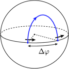
Figure 1: A Giant Magnon solution. The endpoints of the string move on the equator $\theta=\pi/2$ at the speed of light. The magnon momentum is given by $p=\Delta\varphi$, where $\Delta\varphi$ is the angular distance between two endpoints of the string.

The Giant Magnon solution therefore has the following boundary conditions for $Z_{1}$ and $Z_{2}$,

$$Z_{1}\to\exp\left(it\pm i\frac{p}{2}\right)\,,\;\;\;\;\;Z_{2}\to 0,~{}~{}{\mathrm{as}}~{}~{}x\to\pm\infty\,.$$ (12)

In the following we will show that the unique solution with the required properties which satisfies (12) is

$$Z_{1}=\left[\sin\left(\frac{p}{2}\right)\tanh(Y)-i\cos\left(\frac{p}{2}\right)\right]\,\exp(it)\,,\;\;\;\;\;Z_{2}=\frac{\sin\left(\frac{p}{2}\right)}{\cosh(Y)}\,,$$ (13)

where

$$Y=\frac{x-\cos\left(\frac{p}{2}\right)t}{\sin\left(\frac{p}{2}\right)}\,.$$ (14)

This solution is equivalent to the one given as Eqn (2.16) in [9]. We will rederive it as a special case of the more general solution presented below. One may check that while the energy $\Delta$ and the angular momentum $J_{1}$ of the solution diverge, the combination $\Delta-J_{1}$ remains finite and is given by,

$$\Delta-J_{1}=\frac{\sqrt{\lambda}}{\pi}\left|\sin\left(\frac{p}{2}\right)\right|$$ (15)

in agreement with the large-$\lambda$ limit of (1). Moreover the solution (13) carries only one non-vanishing angular momentum, having $J_{2}=0$.

To solve the string equations of motion (9) in the general case, together with the Virasoro conditions (10), we will exploit the equivalence of this system with the CsG equation. Following [12], we will begin by identifying the the $SO(4)$ invariant combinations of the worldsheet fields $\vec{X}$ and their derivatives. As the first derivatives $\partial_{\pm}\vec{X}$ are unit vectors, we can define a real scalar field $\phi(x,t)$ via the relation,

$$\cos\phi=\partial_{+}\vec{X}\cdot\partial_{-}\vec{X}\,.$$ (16)

Taking into account the constraint $|\vec{X}|^{2}=1$, we see that there are no other independent $SO(4)$ invariant quantities that can be constructed out of the fields and their first derivatives. At the level of second derivatives we can construct two additional invariants;

$$u\sin\phi=\partial_{+}^{2}\vec{X}\cdot\vec{K}\,,\;\;\;v\sin\phi=\partial_{-}^{2}\vec{X}\cdot\vec{K}\,,$$ (17)

where the components of vector $\vec{K}$ are given by $K_{i}=\epsilon_{ijkl}X_{j}\partial_{+}X_{k}\partial_{-}X_{l}$. The connection with CsG model arises from the equations of motion for $u$, $v$ and $\phi$ derived in [12]. In fact the resulting equations imply that $u$ and $v$ are not independent and can be eliminated in favour of a new field $\chi(x,t)$ as,

$$u=\partial_{+}\chi\tan\left(\frac{\phi}{2}\right)\,,\;\;\;\;\;v=-\partial_{-}\chi\tan\left(\frac{\phi}{2}\right)\,.$$ (18)

The equations of motion for $\chi$ and $\phi$ can then be written as

$$\partial_{+}\partial_{-}\phi+\sin\phi-\frac{\tan^{2}\left(\frac{\phi}{2}\right)}{\sin\phi}\partial_{+}\chi\partial_{-}\chi=0\,,$$ (19)

$$\partial_{+}\partial_{-}\chi+\frac{1}{\sin\phi}(\partial_{+}\phi\partial_{-}\chi+\partial_{-}\phi\partial_{+}\chi)=0\,.$$ (20)

In the special case of constant $\chi$ they reduce to the usual sine-Gordon equation for $\phi(x,t)$. Finally we can combine the real fields $\phi$ and $\chi$ to form a complex field $\psi=\sin\left(\phi/2\right)\exp(i\chi/2)$, which obeys the equation,

$$\partial_{+}\partial_{-}\psi+\psi^{*}\frac{\partial_{+}\psi\partial_{-}\psi}{1-|\psi|^{2}}+\psi(1-|\psi|^{2})=0\,.$$ (21)

Equation (21) is known as the Complex sine-Gordon equation. Like the ordinary sG equation, it is completely integrable and has localised soliton solutions which undergo factorised scattering. The CsG equation is invariant under a global rotation of the phase of the complex field: $\psi\rightarrow\exp(i\nu)\psi$, $\psi^{*}\rightarrow\exp(-i\nu)\psi^{*}$. In addition to momentum and energy, CsG solitons carry the corresponding conserved $U(1)$ Noether charge. The most general one soliton solution to (21) is given by (see eg [18]),

$$\psi_{\rm 1\mbox{-}soliton} = e^{i\mu}\frac{\cos(\alpha)\exp(i\sin(\alpha)T)}{\cosh(\cos(\alpha)(X-X_{0}))}$$ (22)

with

$$X=\cosh(\theta)x-\sinh(\theta)t\,, T=\cosh(\theta)t-\sinh(\theta)x\,.$$ (23)

The constant phase $\mu$ is irrelevant for our purposes as only the derivatives of the field $\chi$ affect the corresponding string solution. The parameter $X_{0}$ can be absorbed by a constant translation of the world-sheet coordinate $x$ and we will set it to zero. The two remaining parameters of the solution are the rapidity $\theta$ of the soliton and an additional real number $\alpha$ which determines the $U(1)$ charge carried by the soliton.

Taking the limit $\alpha\rightarrow 0$, the field $\phi$ corresponding to the one-soliton solution (22) reduces to the kink solution of the ordinary sG equation. As it is the only known solution of the CsG equation with this property, it is the unique candidate for the dyonic Giant Magnon solution we seek. It remains to reconstruct the corresponding configuration of the string worldsheet fields $\vec{X}$ (or equivalently $Z_{1}$ and $Z_{2}$) corresponding to (22) for general values of the rapidity $\theta$ and rotation parameter $\alpha$.

In this case we have,

$$\partial_{+}\vec{X}\cdot\partial_{-}\vec{X}=\cos(\phi)=1-\frac{2\cos^{2}(\alpha)}{\cosh^{2}\left(\cos(\alpha)X\right)}\,.$$ (24)

Hence the complex coordinates $Z_{1}$ and $Z_{2}$ must both solve the linear equation,

$$\frac{\partial^{2}Z}{\partial t^{2}}-\frac{\partial^{2}Z}{\partial x^{2}}+\left[1-\frac{2\cos^{2}(\alpha)}{\cosh^{2}\left(\cos(\alpha)X\right)}\right]Z = 0$$ (25)

where, as above $X=\cosh(\theta)x-\sinh(\theta)t$ and we impose the boundary conditions appropriate for a Giant Magnon with momentum $p$,

$$Z_{1}\to\exp\left(it\pm i\frac{p}{2}\right)\,\;\;\;\;\;Z_{2}\to 0,~{}~{}{\mathrm{as}}~{}~{}x\to\pm\infty\,.$$ (26)

As always the two complex fields obey the constraint $|Z_{1}|^{2}+|Z_{2}|^{2}=1$. We will find unique solutions of the linear equation (25) obeying these conditions and then, for self-consistency, check that they correctly reproduce (24).

It is convenient to express the solution of (25) in terms of the boosted coordinates $X$ and $T$. In terms of these variables $Z=Z[X,T]$ obeys,

$$\frac{\partial^{2}Z}{\partial T^{2}}-\frac{\partial^{2}Z}{\partial X^{2}}+\left[1-\frac{2\cos^{2}(\alpha)}{\cosh^{2}\left(\cos(\alpha)X\right)}\right]Z = 0\,.$$ (27)

The problem now has the form of a Klein-Gordon equation describing the scattering of a relativistic particle in one spatial dimension incident on a static potential well. As usual the general solution of this equation can be written as a linear combination of “stationary states” of the form,

$$Z_{\omega}=F_{\omega}(X)\exp(i\omega T)\,.$$ (28)

Rescaling the variables according to,

$$\xi=\cos(\alpha)X\,,\,\,\,\,\, f(\xi)=F_{\omega}(X)\,,\,\,\,\,\, \varepsilon=\frac{\sqrt{\omega^{2}-1}}{\cos(\alpha)}\,,$$ (29)

we find that the function $f(\xi)$ obeys the equation,

$$-\frac{d^{2}f}{d\xi^{2}}-\frac{2}{\cosh^{2}(\xi)}\,f=\varepsilon^{2}f\,.$$ (30)

Equation (30) coincides with the time-independent Schrödinger equation for a particle in (a special case of) the Rosen-Morse potential [23],

$$V(\xi)=\frac{-2}{\cosh^{2}(\xi)}\,.$$ (31)

The exact spectrum of this problem is known (see e.g.​ [24]). There is a single normalisable boundstate with energy $\varepsilon^{2}=-1$ and wavefunction,

$$f_{-1}(\xi)=\frac{1}{\cosh(\xi)}$$ (32)

and a continuum of scattering states with $\varepsilon^{2}=k^{2}$ for $k>0$ and wavefunctions,

$$f_{k^{2}}(\xi)=\exp(ik\xi)\left(\tanh(\xi)-ik\right)$$ (33)

with asymptotics,

$$f_{k^{2}}(\xi)\rightarrow\,\,\exp\left(ik\xi\pm i\frac{\delta}{2}\right)$$ (34)

where the scattering phase-shift is given as $\delta=2\tan^{-1}(1/k)$.

The general solution to the original linear equation (25) can be constructed as a linear combination of these boundstate and scattering wavefunctions. The particular solutions corresponding to the worldsheet fields $Z_{1}$ and $Z_{2}$ are singled out by the boundary conditions (26). In particular, the boundary condition (26) can only be matched by a solution corresponding to a single scattering mode $f_{k^{2}}(\xi)$;

$$Z_{1}=c_{1}f_{k^{2}}\left(\cos(\alpha)X\right)\,\exp(i\omega_{k^{2}}T)$$ (35)

where $\omega_{k^{2}}=\sqrt{k^{2}\cos^{2}(\alpha)+1}$. We find that (26) is obeyed provided we set,

$$k=\frac{\sinh(\theta)}{\cos(\alpha)}$$ (36)

which yields the magnon momentum $p=\delta=2\tan^{-1}(1/k)$. The boundary condition (26) dictates that $Z_{2}$ decays at left and right infinity. This is only possible if we identify it with the solution corresponding to the unique normalisable boundstate of the potential (30),

$$Z_{2}=c_{2}f_{-1}(\cos(\alpha)X)\exp(i\omega_{-1}T)$$ (37)

with $\omega_{-1}=\sin(\alpha)$. Without loss of generality we can choose the constants $c_{1}$ and $c_{2}$ to be real. The condition $|Z_{1}|^{2}+|Z_{2}|^{2}=1$ then yields,

$$c_{1}=c_{2}=\frac{1}{\sqrt{1+k^{2}}}\,.$$ (38)

To summarise the above discussion the resulting string solution is,

$$Z_{1} = \frac{1}{\sqrt{1+k^{2}}}\,\,\left(\tanh\left[\cos(\alpha)X\right]-ik\right)\,\,\exp(it)\,,$$

$$Z_{2} = \frac{1}{\sqrt{1+k^{2}}}\,\,\frac{1}{\cosh\left[\cos(\alpha)X\right]}\exp\left(i\sin(\alpha)T\right)\,,$$ (39)

where $X$, $T$ and $k$ are defined in (23) and (36) above. One may easily check that this solution, in addition to obeying the string equation of motion (25) and boundary conditions (26), obeys the Virasoro constraints and satisfies the self-consistency condition (24). It also reduces to the Hofman-Maldacena solution (13) in the non-rotating case $\alpha=0$. Setting $p=\pi$, we obtain one-half of the folded string configuration discussed in [14].

The solution (39) depends on two parameters: $k$ and $\alpha$. We can now evaluate the conserved charges (7) and (8) as a function of these parameters,

$$\Delta-J_{1} = \frac{\sqrt{\lambda}}{\pi}\,\frac{1}{1+k^{2}}\,\,\frac{\sqrt{1+k^{2}\cos^{2}(\alpha)}}{\cos(\alpha)}\,,$$

$$J_{2} = \frac{\sqrt{\lambda}}{\pi}\,\frac{1}{1+k^{2}}\,\,\tan(\alpha)\,.$$ (40)

As above the magnon momentum is identified as $p=2\tan^{-1}(1/k)$. Eliminating $k$ and $\alpha$ we obtain the dispersion relation,

$$\Delta-J_{1} = \sqrt{J_{2}^{2}+\frac{\lambda}{\pi^{2}}\sin^{2}\left(\frac{p}{2}\right)}\,,$$ (41)

which agrees precisely with the BPS dispersion relation (2) for the magnon boundstates obtained in [14].

The time dependence of the solution (39) is also of interest. As in the orginal HM solution the constant phase rotation of $Z_{1}$ with exponent $it$ ensures that the endpoints of the string move on an equator of the three-sphere at the speed of light. We can remove this dependence by changing coordinates from $Z_{1}$ to $\widetilde{Z}_{1}=\exp(-it)Z_{1}$. In the new frame, the string configuration depends periodically on time through the $t$-dependence of $Z_{2}$. The period, ${\cal T}$, for this motion is the time for the solution to come back to itself up to a translation of the worldsheet coordinate $x$. From (39) we find,

$${\cal T}=2\pi\frac{\cosh(\theta)}{\sin(\alpha)}\,.$$ (42)

As we have a periodic classical solution it is natural to define a corresponding action variable. A leading-order semiclassical quantization can then be performed by restricting the action variable to integral values according to the Bohr-Sommerfeld condition. Following [9], the action variable $I$ is defined by the equation,

$$dI=\frac{{\cal T}}{2\pi}\,\left.d(\Delta-J_{1})\right|_{p}\,.$$ (43)

where the subscript $p$ indicates that the differential is taken with fixed $p$. Using (40), (41) and (42) we obtain simply $dI=dJ_{2}$ which is consistent with the identification $I=J_{2}$. This is very natural as we expect the angular momentum $J_{2}$ to be integer valued in the quantum theory. It is also consistent with the semiclassical quantization of finite-gap solutions discussed in [25] where the action variables correspond to the filling fractions. These quantities are simply the number of units of $J_{2}$ carried by each worldsheet excitation.

HYC is supported by a Benefactors’ scholarship from St. John’s College, Cambridge. ND is supported by a PPARC Senior Fellowship.

References

- [1] J. A. Minahan and K. Zarembo, “The Bethe-ansatz for N = 4 super Yang-Mills,” JHEP 0303 (2003) 013 [arXiv:hep-th/0212208].
-
[2]
N. Beisert and M. Staudacher,
“The N = 4 SYM integrable super spin chain,”
Nucl. Phys. B 670 (2003) 439
[arXiv:hep-th/0307042].
N. Beisert, C. Kristjansen and M. Staudacher, “The dilatation operator of N = 4 super Yang-Mills theory,” Nucl. Phys. B 664 (2003) 131 [arXiv:hep-th/0303060]. -
[3]
G. Mandal, N. V. Suryanarayana and S. R. Wadia,
“Aspects of semiclassical strings in AdS(5),”
Phys. Lett. B 543, 81 (2002)
[arXiv:hep-th/0206103].
I. Bena, J. Polchinski and R. Roiban, “Hidden symmetries of the AdS(5) x S**5 superstring,” Phys. Rev. D 69, 046002 (2004) [arXiv:hep-th/0305116]. - [4] N. Beisert, V. Dippel and M. Staudacher, “A novel long range spin chain and planar N = 4 super Yang-Mills,” JHEP 0407 (2004) 075 [arXiv:hep-th/0405001].
- [5] G. Arutyunov, S. Frolov and M. Staudacher, “Bethe ansatz for quantum strings,” JHEP 0410 (2004) 016 [arXiv:hep-th/0406256].
- [6] M. Staudacher, “The factorized S-matrix of CFT/AdS,” JHEP 0505, 054 (2005) [arXiv:hep-th/0412188].
- [7] N. Beisert and M. Staudacher, “Long-range PSU(2,24) Bethe ansaetze for gauge theory and strings,” Nucl. Phys. B 727 (2005) 1 [arXiv:hep-th/0504190].
- [8] N. Beisert, “The su(22) dynamic S-matrix,” arXiv:hep-th/0511082.
- [9] D. M. Hofman and J. M. Maldacena, “Giant magnons,” arXiv:hep-th/0604135.
-
[10]
N. Mann and J. Polchinski,
“Bethe ansatz for a quantum supercoset sigma model,”
Phys. Rev. D 72 (2005) 086002
[arXiv:hep-th/0508232].
J. Ambjorn, R. A. Janik and C. Kristjansen, “Wrapping interactions and a new source of corrections to the spin-chain / string duality,” Nucl. Phys. B 736, 288 (2006) [arXiv:hep-th/0510171].
R. A. Janik, “The AdS(5) x S**5 superstring worldsheet S-matrix and crossing symmetry,” arXiv:hep-th/0603038.
T. Klose and K. Zarembo, “Bethe ansatz in stringy sigma models,” arXiv:hep-th/0603039.
N. Gromov, V. Kazakov, K. Sakai and P. Vieira, “Strings as multi-particle states of quantum sigma-models,” arXiv:hep-th/0603043.
G. Arutyunov and A. A. Tseytlin, “On highest-energy state in the su(11) sector of N = 4 super Yang-Mills arXiv:hep-th/0603113.
G. Arutyunov and S. Frolov, “On AdS(5) x S**5 string S-matrix,” arXiv:hep-th/0604043. -
[11]
A. Santambrogio and D. Zanon,
“Exact anomalous dimensions of N = 4 Yang-Mills operators with large R
charge,”
Phys. Lett. B 545 (2002) 425
[arXiv:hep-th/0206079].
D. Berenstein, D. H. Correa and S. E. Vazquez, “All loop BMN state energies from matrices,” JHEP 0602 (2006) 048 [arXiv:hep-th/0509015]. - [12] K. Pohlmeyer, “Integrable Hamiltonian Systems And Interactions Through Quadratic Constraints,” Commun. Math. Phys. 46 (1976) 207.
-
[13]
A. Mikhailov,
“An action variable of the sine-Gordon model,”
arXiv:hep-th/0504035.
A. Mikhailov, “A nonlocal Poisson bracket of the sine-Gordon model,” arXiv:hep-th/0511069. - [14] N. Dorey, “Magnon bound states and the AdS/CFT correspondence,” arXiv:hep-th/0604175.
- [15] S. Frolov and A. A. Tseytlin, “Rotating string solutions: AdS/CFT duality in non-supersymmetric sectors,” Phys. Lett. B 570 (2003) 96 [arXiv:hep-th/0306143].
- [16] G. Arutyunov, S. Frolov, J. Russo and A. A. Tseytlin, “Spinning strings in AdS(5) x S**5 and integrable systems,” Nucl. Phys. B 671 (2003) 3 [arXiv:hep-th/0307191].
-
[17]
F. Lund and T. Regge,
“Unified Approach To Strings And Vortices With Soliton Solutions,”
Phys. Rev. D 14 (1976) 1524.
F. Lund, “Example Of A Relativistic, Completely Integrable, Hamiltonian System,” Phys. Rev. Lett. 38 (1977) 1175.
B. S. Getmanov, “Integrable Model For The Nonlinear Complex Scalar Field With The Nontrivial Asymptotics Of N - Soliton Solutions,” Theor. Math. Phys. 38 (1979) 124 [Teor. Mat. Fiz. 38 (1979) 186].
B. S. Getmanov, “Integrable Two-Dimensional Lorentz Invariant Nonlinear Model Of Complex Scalar Field (Complex Sine-Gordon Ii),” Theor. Math. Phys. 48 (1982) 572 [Teor. Mat. Fiz. 48 (1981) 13].
H. J. de Vega and J. M. Maillet, “Renormalization Character And Quantum S Matrix For A Classically Integrable Theory,” Phys. Lett. B 101 (1981) 302.
H. J. de Vega and J. M. Maillet, “Semiclassical Quantization Of The Complex Sine-Gordon Field Theory,” Phys. Rev. D 28 (1983) 1441. - [18] N. Dorey and T. J. Hollowood, “Quantum scattering of charged solitons in the complex sine-Gordon model,” Nucl. Phys. B 440 (1995) 215 [arXiv:hep-th/9410140].
- [19] P. Bowcock and G. Tzamtzis, “The complex sine-Gordon model on a half line,” arXiv:hep-th/0203139.
- [20] B. Julia and A. Zee, “Poles With Both Magnetic And Electric Charges In Nonabelian Gauge Theory,” Phys. Rev. D 11, 2227 (1975).
- [21] E. Tomboulis and G. Woo, “Semiclassical Quantization For Gauge Theories,” MIT-CTP-540
- [22] E. Witten and D. I. Olive, “Supersymmetry Algebras That Include Topological Charges,” Phys. Lett. B 78 (1978) 97.
- [23] N. Rosen and P. Morse, Phys. Rev. 42 (1932) 210.
- [24] L. D. Landau, E. M. Lifshitz, “Quantum Mechanics (Non-Relativistic Theory)” (Pergamon), p.73 Problem 5 and p.80 Problem 4.
- [25] N. Dorey and B. Vicedo, “On the dynamics of finite-gap solutions in classical string theory,” arXiv:hep-th/0601194.