POLARIZATION CORRELATIONS IN MUON PAIR PRODUCTION IN THE ELECTROWEAK MODEL

Abstract

Explicit field theory computations are carried out of the joint probabilities associated with spin correlations of $\mu^{-}\mu^{+}$ produced in $e^{-}e^{+}$ collision in the standard electroweak model to the leading order. The derived expressions are found to depend not only on the speed of the $e^{-}e^{+}$ pair but also on the underlying couplings. These expressions are unlike the ones obtained from simply combining the spins of the relevant particles which are of kinematical nature. It is remarkable that these explicit results obtained from quantum field theory show a clear violation of Bell’s inequality.

Received 11 October 2005Revised 26 October 2005

Keywwords: Polarization correlations, Quantum field theory, High-Energy computation, The Standard Electroweak Model, Bell’s test

PACS Nos.: 11.15Bt, 12.15Ji, 13.88.+e, 03.65.Ud

Several experiments have been performed over the years on particles’ polarizations correlations [1, 2, 3, 4, 5] in the light of Bell’s inequality and many Bell-like experiments have been proposed recently in high energy physics. [6, 7, 8, 9, 10, 11] We have been particularly interested in actual quantum field theory computations of polarizations correlations probabilities of particles produced in basic processes because of novelties encountered in dynamical calculations as opposed to kinematical considerations to be discussed. Here it is worth recalling that quantum field theory originates from the combination of quantum physics and relativity and involve non-trivial dynamics. Many such computations have been done in QED [12, 13] as well as in $e^{-}e^{+}$ pair production from some charged and neutral strings [14]. All of these polarizations correlations probabilities based on dynamical analyses following from field theory share the interesting property that they depend on the energy (speeds) of the colliding particles due to the mere fact that typically the latter carry speeds in order to collide. Such analyses are unlike considerations based on formal arguments of simply combining spins [17], as is usually done, and are of kinematical nature, void of dynamical considerations. Here it is worth recalling that the total spin of a two-particle system each with spin, such as of two spin $1/2$’s, is obtained not only from combining the spins of the latter but also from any orbital angular momentum residing in their center of mass system. For low speeds, one expects that the argument based simply on combining the spins of the colliding particles should provide an accurate description of the polarization correlations sought and all of our QED computations [12, 13] show the correctness of such an argument in the limit of low speeds. Needless to say, we are interested in the relativistic regime as well, and the formal arguments just mentioned fail to provide the correct expressions for the correlations. As a byproduct of the work, our computations of the joint polarizations correlations carried out in a full quantum field theory setting show a clear violation of Bell’s inequality.

In the present communication we encounter additional completely novel properties not encountered in our earlier QED [12, 13] calculations. We consider the process $e^{-}e^{+}\to\mu^{-}\mu^{+}$ as described in the standard electroweak (EW) model. It is well known that this process [15] as computed in the EW model is in much better agreement with experiments than that of a QED computation. The reasons for considering such a process in the EW model are many, one of which is the high precision of the differential cross section obtained as just discussed. Reasons which are, however, more directly relevant to our anylyses are the following. Due to the theshold energy needed to create the $\mu^{-}\mu^{+}$ pair, the limit of the speed $\beta$ of the colliding particles cannot be taken to go to zero. This is unlike processes treated by the authors in QED such as in $e^{-}e^{-}\to{}e^{-}e^{-}$, $e^{+}e^{-}\to 2\gamma$, Therefore all arguments based simply on combining the spins of $e^{-}$, $e^{+}$, without dynamical considerations, fail. [As a matter of fact the latter argument would lead for the joint probability in (7) we are seeking, the incorrect result $(1/2)\sin^{2}\left(\left(\chi_{1}-\chi_{2}\right)/2\right)$—an expression which has been used for years.] Another novelty we encounter in the present investigation is that the polarization correlations not only depend on speed but have also an explicit dependence on the underlying couplings. Again this latter explicit dependence is unlike the situation arising in QED [12, 13].

The relevant quantity of interest here in testing Bell’s inequality [16, 17] is, in a standard notation,

$$S =\frac{p_{12}(a_{1},a_{2})}{p_{12}(\infty,\infty)}-\frac{p_{12}(a_{1},a^{\prime}_{2})}{p_{12}(\infty,\infty)}+\frac{p_{12}(a^{\prime}_{1},a_{2})}{p_{12}(\infty,\infty)}+\frac{p_{12}(a^{\prime}_{1},a^{\prime}_{2})}{p_{12}(\infty,\infty)}$$

$$\quad-\frac{p_{12}(a^{\prime}_{1},\infty)}{p_{12}(\infty,\infty)}-\frac{p_{12}(\infty,a_{2})}{p_{12}(\infty,\infty)}$$ (1)

as is computed from the electroweak model. Here $a_{1}$, $a_{2}$  $(a^{\prime}_{1},a^{\prime}_{2})$ specify directions along which the polarizations of two particles are measured, with $p_{12}(a_{1},a_{2})/p_{12}(\infty,\infty)$ denoting the joint probability, and $p_{12}(a_{1},\infty)/p_{12}(\infty,\infty)$, $p_{12}(\infty,a_{2})/p_{12}(\infty,\infty)$ denoting the probabilities when the polarization of only one of the particles is measured. [$p_{12}(\infty,\infty)$ is a normalization factor.] The corresponding probabilities as computed from the electroweak model will be denoted by $P(\chi_{1},\chi_{2})$, $P(\chi_{1},-)$, $P(-,\chi_{2})$ with $\chi_{1}$, $\chi_{2}$ denoting angles specifying directions along which spin measurements are carried out with respect to certain axes spelled out in the bulk of the paper. To show that the electroweak model is in violation with Bell’s inequality of LHV, it is sufficient to find one set of angles $\chi_{1}$, $\chi_{2}$, $\chi^{\prime}_{1}$, $\chi^{\prime}_{2}$, such that $S$, as computed in the electroweak model, leads to a value of $S$ outside the interval $[-1,0]$. In this work, it is implicitly assumed that the polarization parameters in the particle states are directly observable and may be used for Bell-type measurements as discussed.

We consider the process $e^{-}e^{+}\to\mu^{-}\mu^{+}$ in the center of mass frame (see figure 1) with the momentum of, say, $e^{-}$ chosen to be $\boldsymbol{\mathrm{p}}=\gamma\beta{}m_{e}\big{(}0,1,0\big{)}={-}\boldsymbol{\mathrm{k}}$, $m_{e}$ denoting its mass and $\gamma=1/\sqrt{1-\beta^{2}}$. The momentum of the emerging $\mu^{-}$ will be taken to be $\boldsymbol{\mathrm{p}}^{\prime}=\gamma^{\prime}\beta^{\prime}m_{\mu}\big{(}1,0,0\big{)}={-}\boldsymbol{\mathrm{k}}^{\prime}$, $\gamma^{\prime}=1/\sqrt{1-\beta^{\prime 2}}$, and $m_{\mu}$ is the mass of $\mu^{-}(\mu^{+})$, the spinors of $e^{-}$, $e^{+}$ are chosen as

$$u(p)=\sqrt{\frac{\gamma+1}{2}}\begin{pmatrix}\uparrow\\ \mathrm{i}\frac{\gamma\beta}{\gamma+1}\downarrow\end{pmatrix}\quad\text{and}\quad v(k)=\sqrt{\frac{\gamma+1}{2}}\begin{pmatrix}\mathrm{i}\frac{\gamma\beta}{\gamma+1}\uparrow\\ \downarrow\end{pmatrix}.$$ (2)

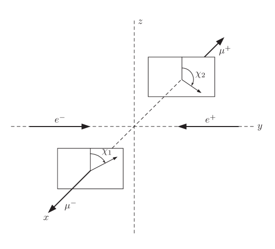
Figure 1: The figure depicts the process $e^{-}e^{+}\to\mu^{-}\mu^{+}$, with $e^{-}$, $e^{+}$ moving along the $y$–axis, and the emerging muons moving along the $x$–axis. $\chi_{1}$ and $\chi_{2}$ denote the angles with the $z$–axis specifying the directions of measurements of the spins of $\mu^{-}$ and $\mu^{+}$, respectively.

Obviously, there is a non-zero probability of occurrence of the above process. Given that such a process has occurred, we compute the conditional joint probability of spins measurements of $\mu^{-}$, $\mu^{+}$ along directions specified by the angles $\chi_{1}$, $\chi_{2}$ as shown in figure 1. Here we have considered the so-called singlet state. The triplet state leads to an expression similar to the one in (7) for the probability in question with different coefficients $A(\mathcal{E})$, $\ldots$, $E(\mathcal{E})$, $N(\mathcal{E})$ and leads again to a violation of Bell’s inequality. The corresponding details may be obtained from the authors by the interested reader.

A fairly tedious computation for the invariant amplitude of the process [18, 19, 20] in figure 1 leads to

$$\mathcal{M} \propto\left[A(\mathcal{E})\sin\left(\frac{\chi_{1}-\chi_{2}}{2}\right)+B(\mathcal{E})\sin\left(\frac{\chi_{1}+\chi_{2}}{2}\right)+C(\mathcal{E})\cos\left(\frac{\chi_{1}-\chi_{2}}{2}\right)\right]$$

$$\qquad-\mathrm{i}\left[D(\mathcal{E})\sin\left(\frac{\chi_{1}+\chi_{2}}{2}\right)+E(\mathcal{E})\cos\left(\frac{\chi_{1}-\chi_{2}}{2}\right)\right]$$ (3)

where

$$A(\mathcal{E}) =\left(\frac{M^{2}_{Z}}{4\mathcal{E}^{2}}+ab^{2}-1\right)$$ (4a)

$$B(\mathcal{E}) ={-}\left(\frac{m_{e}}{m_{\mu}}\right)\left(\frac{M^{2}_{Z}}{4\mathcal{E}^{2}}+ab^{2}-1\right)$$ (4b)

$$C(\mathcal{E}) =\frac{abm_{e}}{\mathcal{E}m_{\mu}}\sqrt{\mathcal{E}^{2}-m^{2}_{\mu}}$$ (4c)

$$D(\mathcal{E}) =\frac{a}{m_{\mu}\mathcal{E}}\sqrt{\mathcal{E}^{2}-m^{2}_{\mu}}\>\sqrt{\mathcal{E}^{2}-m^{2}_{e}}$$ (4d)

$$E(\mathcal{E}) ={-}\frac{ab}{m_{\mu}}\sqrt{\mathcal{E}^{2}-m^{2}_{e}}$$ (4e)

and

$$a\equiv\dfrac{g^{2}}{16e^{2}\cos^{2}\theta_{\mathrm{W}}}\cong{}0.353,\qquad b\equiv 1-4\sin^{2}\theta_{\mathrm{W}}\cong{}0.08$$ (4f)

$g$ denotes the weak coupling constant, $\theta_{\mathrm{W}}$ is the Weinberg angle, and $e$ denotes the electric charge. The contribution of the Higgs particles turns out to be too small and is negligible. [19]

Using the notation $F(\chi_{1},\chi_{2})$ for the absolute value squared of the right-hand side of (3), the conditional joint probability distribution of spin measurements along the directions specified by the angles $\chi_{1}$, $\chi_{2}$ is given by

$$P(\chi_{1},\chi_{2})=\frac{F(\chi_{1},\chi_{2})}{N(\mathcal{E})}$$ (5)

where the normalization factor $N(\mathcal{E})$ is

$$N(\mathcal{E}) \equiv{}F(\chi_{1},\chi_{2})+F(\chi_{1}+\pi,\chi_{2})+F(\chi_{1},\chi_{2}+\pi)+F(\chi_{1}+\pi,\chi_{2}+\pi)$$

$$=2\Big{\{}\big{[}A(\mathcal{E})\big{]}^{2}+\big{[}B(\mathcal{E})\big{]}^{2}+\big{[}C(\mathcal{E})\big{]}^{2}+\big{[}D(\mathcal{E})\big{]}^{2}+\big{[}E(\mathcal{E})\big{]}^{2}\Big{\}}$$ (6)

giving

$$P(\chi_{1},\chi_{2}) =\frac{1}{N(\mathcal{E})}\left[A(\mathcal{E})\sin\left(\frac{\chi_{1}-\chi_{2}}{2}\right)+B(\mathcal{E})\sin\left(\frac{\chi_{1}+\chi_{2}}{2}\right)+C(\mathcal{E})\cos\left(\frac{\chi_{1}-\chi_{2}}{2}\right)\right]^{2}$$

$$\quad+\frac{1}{N(\mathcal{E})}\left[D(\mathcal{E})\sin\left(\frac{\chi_{1}+\chi_{2}}{2}\right)+E(\mathcal{E})\cos\left(\frac{\chi_{1}-\chi_{2}}{2}\right)\right]^{2}.$$ (7)

The probabilities associated with the measurement of only one of the polarizations are given respectively, by

$$P(\chi_{1},-)=\frac{1}{2}-\frac{2B(\mathcal{E})}{N(\mathcal{E})}\big{[}A(\mathcal{E})\cos\chi_{1}+C(\mathcal{E})\sin\chi_{1}\big{]}$$ (8)

and similarly for $\chi_{2}$

$$P(-,\chi_{2})=\frac{1}{2}+\frac{2B(\mathcal{E})}{N(\mathcal{E})}\big{[}A(\mathcal{E})\cos\chi_{2}+C(\mathcal{E})\sin\chi_{2}\big{]}.$$ (9)

It is important to note that $P(\chi_{1},\chi_{2})\neq{}P(\chi_{1},-)P(-,\chi_{2})$, in general, showing the obvious correlations occurring between the two spins.

The indicator $S$ in (1) computed according to the probabilities $P(\chi_{1},\chi_{2})$, $P(\chi_{1},-)$, $P(-,\chi_{2})$ in (7), (8), (9) may be readily evaluated. To show violation of Bell’s inequality, it is sufficient to find four angles $\chi_{1}$, $\chi_{2}$, $\chi^{\prime}_{1}$, $\chi^{\prime}_{2}$ at accessible energies, for which $S$ falls outside the interval $[{-}1,0]$. For $\mathcal{E}=105.656$ MeV, i.e., near threshold, an optimal value of $S$ is obtained equal to $-1.28203$, for $\chi_{1}=0^{\circ}$, $\chi_{2}=45^{\circ}$, $\chi^{\prime}_{1}=90^{\circ}$, $\chi^{\prime}_{2}=135^{\circ}$, clearly violating Bell’s inequality. For the energies originally carried out in the experiment on the differential cross section at $\mathcal{E}\sim 34$ GeV, an optimal value of $S$ is obtained equal to $-1.22094$ for $\chi_{1}=0^{\circ}$, $\chi_{2}=45^{\circ}$, $\chi^{\prime}_{1}=51.13^{\circ}$, $\chi^{\prime}_{2}=170.85^{\circ}$.

As mentioned in the introductory part of the paper, one of the reasons for this investigation arose from the fact that the limit of the speed $\beta$ of $e^{-}e^{+}$ cannot be taken to go to zero due to the threshold energy needed to create the $\mu^{-}\mu^{+}$ pair and methods used for years by simply combining the spins of the particles in question completely fail. The present computations are expected to be relevant near the threshold energy for measuring the spins of the $\mu^{-}\mu^{+}$ pair. Near the threshold, the indicator $S_{\mathrm{QED}}$ computed within QED coincides with that of $S$ given above in the electroweak model, and varies slightly at higher energies, thus confirming that the weak effects are negligible. Due to the persistence of the dependence of the indicator $S$ on speed, as seen above, in a non-trivial way, it would be interesting if any experiments may be carried out to assess the accuracy of the indicator $S$ as computed within (relativistic) quantum field theory. As there is ample support of the dependence of polarizations correlations, as we have shown by explicit computations in quantum field theory in the electroweak interaction as well as QED ones, [12, 13] on speed, we hope that some new experiments will be carried out in the light of Bell-like tests which monitor speed as further practical tests of quantum physics in the relativistic regime.

References

-
[1]
V. D. Irby, Phys. Rev. A 67, 034102 (2003).
[arXiv: quant-ph/0209158] - [2] S. Osuch, M. Popkiewicz, Z. Szeflinski and Z. Wilhelmi, Acta Phys. Pol. B 27, 567 (1996).
- [3] L. R. Kaday, J. D. Ulman and C. S. Wu, Nuovo Cimento B 25, 633 (1975).
- [4] E. S. Fry, Quantum Semiclass. Opt. 7, 229 (1995).
- [5] A. Aspect, J. Dalibard, and G. Roger, Phys. Rev. Lett. 49, 1804 (1982).
- [6] A. Go, J. Mod. Opt. 51, 991 (2004).
- [7] R. A. Bertlmann, A. Bramon, G. Garbarino and B. C. Hiesmayr, Phys. Lett. A 332, 355 (2004).
- [8] S. A. Abel, M. Dittmar and H. Dreiner, Phys. Lett. B 280, 304 (1992).
- [9] P. Privitera, Phys. Lett. B 275, 172 (1992).
- [10] R. Lednický and V. L. Lyuboshitz, Phys. Lett. B 508, 146 (2001).
- [11] M. Genovese, C. Novero and E. Predazzi, Phys. Lett. B 513, 401 (2001).
-
[12]
N. Yongram and E. B. Manoukian,
Int. J. Theor. Phys. 42, 1755 (2003).
[arXiv: quant-ph/0411072] -
[13]
E. B. Manoukian and N. Yongram,
Eur. Phys. J. D 31, 137 (2004).
[arXiv: quant-ph/0411079] -
[14]
E. B. Manoukian and N. Yongram,
Mod. Phys. Lett. A 20, 623 (2005).
[arXiv: hep-th/0504195] - [15] M. Althoff et al. (TASSO Collaboration), Z. Phys. C 22, 13 (1984).
- [16] J. F. Clauser and M. A. Horne, Phys. Rev. D 10, 526 (1984).
- [17] J. F. Clauser and A. Shimony, Rep. Prog. Phys. 41, 1881 (1978).
- [18] E. D. Commins and P. H. Bucksbaum, Weak Interactions of Leptons and Quarks, Cambridge University Press (New York, 1983).
- [19] W. Greiner and B. Müller,Gauge Theory of Weak Interactions, 2nd edition, Springer (Berlin, 1996).
- [20] P. Renton, Electroweak Interactions: An Introduction to the Physics of Quarks and Leptons, Cambridge University Press (Cambridge, 1990).