We employ analytical methods to study deconstruction of 5D gauge theories in the ${\mathrm{A}\mathrm{d}\mathrm{S}}_{5}$ background. We demonstrate that using the so-called q-Bessel functions allows a quantitative analysis of the deconstructed setup. Our study clarifies the relation of deconstruction with 5D warped theories.

1 Introduction

The framework introduced by Randall and Sundrum in ref. [1] has been playing an important role in high-energy physics in the last years. The Randall–Sundrum setup involves 5D spacetime with the line element

$$ds^{2}=a^{2}(x_{5})dx_{\mu}dx^{\mu}-dx_{5}^{2}\,,$$ (1)

and the fifth dimension truncated at $x_{5}=0$ by the ultraviolet (UV) brane and at $x_{5}=L$ by the infrared (IR) brane. The scale (warp) factor multiplying the 4D Minkowski background metric varies along the fifth dimension, which generates a hierarchy of scales of order $a(0)/a(L)$ between the UV and the IR branes. For example, for the ${\mathrm{A}\mathrm{d}\mathrm{S}}_{5}$ spacetime the warp factor varies exponentially and a huge hierarchy can easily be generated.

The original motivation was to explain in this way the hierarchy between the Planck scale and the electroweak scale. However it has become clear that the scope of application is much wider. In particular, it is interesting to consider situations where the gravitational degrees of freedom can be decoupled. In this case one deals with 5D theories of gauge and matter fields in a fixed background of the form of eq. (1). This approach has turned out to be fruitful for constructing realistic models of the Higgs sector [2], Higgsless electroweak breaking [3] and supersymmetry breaking [4]. Furthermore, AdS/CFT [5] applied to the Randall–Sundrum background [6] suggests that these models are dual descriptions of purely four-dimensional strongly coupled physics. There is also a connection between field-theoretical 5D gauge theories in warped backgrounds and the low-energy physics of pions and vector resonances [7], known as AdS/QCD.

Gauge theories in $D>4$ dimensions possess an intrinsic cutoff scale. The gauge coupling $g_{D}$ has dimension $[{\rm length}]^{D/2-2}$; therefore at high energies scattering amplitudes grow as $E^{D/2-2}$, leading to strong coupling in the UV. Perturbative computations have to be cut off below the strong coupling scale. In some phenomenological applications strong coupling occurs, in fact, not far from the TeV scale. Thus it is often desirable to consider a UV completion of higher dimensional theories so as to understand possible cutoff effects. Typically, this UV completion is assumed to be some sort of string theory.

Deconstruction [8] is another option to model cutoff effects in higher dimensional gauge theories. It is a four-dimensional framework that typically involves a product gauge group $G^{N}$ and a set of bifundamental Higgs fields (the links). With an appropriate choice of representations and vev’s of the links, such a setup, at low energies, reproduces the spectrum and interactions of a higher-dimensional gauge theory with the gauge group $G$. The matching holds up to a certain deviation scale $\Lambda_{D}$, related to the magnitude of the link vev’s. This deviation scale is identified with the cutoff of the higher-dimensional theory. Above $\Lambda_{D}$, deconstruction provides a UV completion in terms of a purely four-dimensional, weakly coupled and, possibly, renormalizable gauge theory dynamics.

Deconstruction of 5D gauge theories in the ${\mathrm{A}\mathrm{d}\mathrm{S}}_{5}$ Randall–Sundrum background was considered in refs. [9, 10, 11, 12, 13]. The warped fifth dimension was represented by a chain of bifundamental links $\Phi_{j}$ with the vev varying as $\langle\Phi_{j}\rangle\sim q^{j}$. This setup turned out to be useful for clarifying several issues concerning the evolution of gauge couplings in ${\mathrm{A}\mathrm{d}\mathrm{S}}_{5}$ [10, 11, 12]. However, these studies suffer from certain limitations. While computations in ${\mathrm{A}\mathrm{d}\mathrm{S}}_{5}$ can be performed (both at the tree level and at the loop level) using familiar Bessel functions, no analytical methods have been available so far to handle computations in the deconstructed model. In particular, the spectrum and interactions of the massive gauge bosons have been determined only numerically. Some analytical results have been obtained, but only for $q\ll 1$, in which case deconstruction does not have an obvious 5D interpretation. For this reason the relation between deconstruction and the ${\mathrm{A}\mathrm{d}\mathrm{S}}_{5}$ theory was somewhat obscure. It was not even clear if deconstruction could really reproduce the ${\mathrm{A}\mathrm{d}\mathrm{S}}_{5}$ physics in its entire perturbativity range. Furthermore, because of these technical problems, the deconstructed ${\mathrm{A}\mathrm{d}\mathrm{S}}_{5}$ setup has not been really useful for phenomenological applications.

In this paper we fill this gap. We present analytical methods to handle deconstructed ${\mathrm{A}\mathrm{d}\mathrm{S}}_{5}$ models. The tools are provided by the mathematical theory of q-difference equations and their solutions. One of its branches deals with the so-called q-Bessel functions, which generalize the ordinary Bessel functions. We show that the q-Bessel functions are appropriate to describe the spectrum and interactions of the deconstructed ${\mathrm{A}\mathrm{d}\mathrm{S}}_{5}$ models. With these methods at hand, the calculabilities of the ${\mathrm{A}\mathrm{d}\mathrm{S}}_{5}$ gauge theory and its deconstructed version stand on an equal footing.

The technical results we obtain help to clarify the relation between the 5D warped gauge theories and deconstruction. It was argued in the previous works [10, 11] that deconstruction realizes a position-dependent cutoff. With the new methods at our disposal we are able to make this notion more precise and specify the parameter range in which deconstruction adequately approximates the 5D theory. The position-dependent cutoff is realized in the following sense. The IR brane scattering amplitudes in the 5D theory are reproduced up to the scale $\Lambda_{\mathrm{I}R}=\Lambda a(L)$. On the other hand, the UV brane t-channel amplitudes are reproduced up to $\Lambda_{\mathrm{U}V}=\Lambda a(0)$, larger by the factor $a(0)/a(L)$. The non-trivial thing about the latter result is that the spectra of massive excitations in the two theories deviate at a much lower scale, of order $\Lambda_{\mathrm{I}R}$. Matching of the UV brane t-channel amplitudes in the two theories holds in spite of the fact that the number and the couplings of the exchanged massive gauge bosons are different. Our results also imply that, up to the scale $\Lambda_{\mathrm{U}V}$, the holographic interpretation of the deconstructed ${\mathrm{A}\mathrm{d}\mathrm{S}}_{5}$ models is similar to that established in [6] for the 5D models.

The paper is organized as follows. In Section 2 we review the necessary technical material concerning gauge theories in ${\mathrm{A}\mathrm{d}\mathrm{S}}_{5}$. In Section 3 we study the deconstructed model and derive analytical formulas for the spectrum and propagators of the gauge bosons. The detailed discussion of these results and their consequences is presented in Section 4. Section 5 contains a summary and points at future applications of our results. Deconstruction of 5D gauge theories with most general boundary conditions is discussed in Appendix A. Finally, Appendix B contains a detailed and self-contained review of the theory of q-Bessel functions.

2 Review of gauge theory in ${\rm AdS}_{5}$

In this section we summarize basic properties of 5D gauge theories in the Randall–Sundrum-type background. The fifth dimension is an interval (equivalently, the orbifold $S^{1}/Z_{2}$) parametrized by $x_{5}\in[0,L]$. Two boundary branes are located at $x_{5}=0$ (the UV brane) and at $x_{5}=L$ (the IR brane). The gravitational background is that of the ${\mathrm{A}\mathrm{d}\mathrm{S}}_{5}$ geometry:

$$ds^{2}=a^{2}(x_{5})\eta_{\mu\nu}dx_{\mu}dx_{\nu}-dx_{5}^{2}\qquad\qquad a(x_{5})=e^{-kx_{5}}\,,$$ (2)

where $k$ is the curvature scale and $\mu,\nu,\dots=0\dots 3$ label the 4D coordinates. The presence of the warp factor generates a hierarchy of scales of order ${1/a_{L}}$ between the UV and the IR brane, where $a_{L}\equiv a(L)=e^{-kL}$. In the original Randall–Sundrum model $a_{L}\sim 10^{-15}$, so as to explain the hierarchy between the electroweak and the Planck scale. In our analysis we allow for arbitrary $a_{L}\ll 1$.

In the following we will focus on the dynamics of gauge theories on such a background, while fluctuations of the 5D metric will be ignored. The practical reason is that deconstruction of gravity encounters certain technical problems [14, 15], which we prefer to avoid here. Formally speaking, gravity can always be decoupled by taking the limit $M_{5}\to\infty$, where $M_{5}$ is the 5D Planck scale. More precisely, gravity couples strongly at the IR brane at the scale $\Lambda_{G}(L)\sim a_{L}M_{\mathrm{P}lanck}\sim a_{L}M_{5}^{3/2}/k^{1/2}$, while at the UV brane it becomes strongly coupled only at $\Lambda_{G}(0)\sim M_{\mathrm{P}lanck}$. We assume we always deal with energies far below the respective gravity strong-coupling scales, and concentrate exclusively on the dynamics of the gauge sector.

We consider a 5D gauge field $A_{M}=(A_{\mu},A_{5})$ propagating in the background of eq. (2). The quadratic part of the action takes the form

$$S_{5}=\int d^{4}x\int_{0}^{L}dx_{5}{1\over g_{5}^{2}}\left(-{1\over 4}F_{\mu\nu}F_{\mu\nu}+{a^{2}(x_{5})\over 2}(\partial_{5}A_{\mu}-\partial_{\mu}A_{5})^{2}\right)\,.$$ (3)

We choose the boundary conditions as

$$\partial_{5}A_{\mu}(0)=\partial_{5}A_{\mu}(L)=0\qquad\qquad A_{5}(0)=A_{5}(L)=0\,.$$ (4)

The Neumann boundary conditions for $A_{\mu}$ allow the existence of a 4D zero mode, so that 4D gauge symmetry survives below the compactification scale. Alternatively, one can impose Dirichlet boundary conditions for $A_{\mu}$ (and Neumann for $A_{5}$), in which case gauge symmetry is entirely broken at low energies. For completeness we review this case and its deconstructed version in Appendix A.

2.1 Spectrum and propagators

There are several ways of approaching higher dimensional theories. Most often, higher dimensional fields are traded for an infinite number of 4D Kaluza–Klein (KK) modes. Another approach relies on 5D propagators, which effectively sum up the contribution of the whole KK tower. Finally, it is sometimes useful to employ the so-called holographic approach, which consists in constructing an effective action for the boundary values of the bulk fields. Below we review the necessary technical background for each approach. Of course, these are merely different methods of organizing computations, and physical conclusions must be the same, regardless of which approach is used.

2.1.1 Kaluza–Klein approach

The gauge field is decomposed into KK modes as follows

$$A_{\mu}(x,x_{5})=\sum_{n=0}^{\infty}f_{n}(x_{5})A_{\mu}^{n}(x)\qquad,\qquad A_{5}(x,x_{5})=\sum_{n=1}^{\infty}{\partial_{5}f_{n}(x_{5})\over m_{n}}A_{5}^{n}(x)\,.$$ (5)

The modes $A_{5}^{n}$ are eaten by the massive gauge fields but it is not necessary to fix the gauge at this stage. The KK profiles $f_{n}$ should be chosen such that the quadratic action (3) is diagonal in the KK basis:

$$S_{5}=\int d^{4}x\sum_{n}\left(-{1\over 4}F_{\mu\nu}^{n}F_{\mu\nu}^{n}+{1\over 2}(m_{n}A_{\mu}^{n}-\partial_{\mu}A_{5}^{n})^{2}\right)\,.$$ (6)

This is obtained when $f_{n}$ are solutions of the equation of motion

$$\partial_{5}^{2}f_{n}-2k\partial_{5}f_{n}+m_{n}^{2}a^{-2}(x_{5})f_{n}=0\,,$$ (7)

satisfy the Neumann boundary conditions

$$\partial_{5}f_{n}(0)=\partial_{5}f_{n}(L)=0\,,$$ (8)

and are normalized as $g_{5}^{-2}\int_{0}^{L}f_{n}^{2}=1$. The solution is given by [16]

$$\displaystyle f_{0} = {g_{5}\over\sqrt{L}}\,,$$

$$\displaystyle f_{n} = A_{n}a^{-1}(x_{5})\left[Y_{0}\left({m_{n}\over k}\right)J_{1}\left({m_{n}\over ka(x_{5})}\right)-J_{0}\left({m_{n}\over k}\right)Y_{1}\left({m_{n}\over ka(x_{5})}\right)\right]\,,\qquad n>0\,,$$ (9)

with the normalization constant

$$A_{n}={\pi m_{n}g_{5}\over\sqrt{2k}}\left(\left({J_{0}({m_{n}\over k})\over J_{0}({m_{n}\over ka_{L}})}\right)^{2}-1\right)^{-1/2}={\pi m_{n}g_{5}\over\sqrt{2k}}\left(\left({Y_{0}({m_{n}\over k})\over Y_{0}({m_{n}\over ka_{L}})}\right)^{2}-1\right)^{-1/2}\,.$$ (10)

Thus, the 5D gauge theory is rewritten in terms of a tower of 4D vector fields $A_{\mu}^{n}$ with masses $m_{n}$ ($A_{5}^{n}$’s are eaten). The zero mode $A_{\mu}^{0}$ corresponds to $m_{0}=0$. Its profile $f_{0}$ is a constant, thus the massless mode couples to all matter with equal strength given by $g_{0}=g_{5}/\sqrt{L}$. For the massive modes, the mass spectrum is given by solutions of the equation

$$Y_{0}\left({m_{n}\over k}\right)J_{0}\left({m_{n}\over ka_{L}}\right)-J_{0}\left({m_{n}\over k}\right)Y_{0}\left({m_{n}\over ka_{L}}\right)=0\,,$$ (11)

which can be well approximated by

$$m_{n}\approx\pi ka_{L}(n-1/4)\,.$$ (12)

The spectrum is approximately linearly spaced with the mass gap $M_{\mathrm{K}K}\sim ka_{L}$. The massive modes couple non-universally to matter, the coupling depending on both the KK number and the position in the extra dimension. In particular, the couplings to the UV and IR branes are determined by the boundary values of the KK profiles

$$f_{n}(0)={\sqrt{2k}g_{5}\over\sqrt{\left({Y_{0}({m_{n}\over k})\over Y_{0}({m_{n}\over ka_{L}})}\right)^{2}-1}}\,,\qquad\qquad f_{n}(L)={\sqrt{2k}g_{5}\left({Y_{0}({m_{n}\over k})\over Y_{0}({m_{n}\over ka_{L}})}\right)\over\sqrt{\left({Y_{0}({m_{n}\over k})\over Y_{0}({m_{n}\over ka_{L}})}\right)^{2}-1}}\,.$$ (13)

Approximating the Bessel functions we find $|f_{n}(L)|^{2}\approx 2kg_{5}^{2}$, so that all the KK modes couple to the IR brane with approximately equal strength. On the other hand $|f_{n}(0)|^{2}\approx 2ka_{L}g_{5}^{2}(\pi k/2m_{n})\log^{-2}(m_{n}/k)$ for $m_{n}\ll k$ and $|f_{n}(0)|^{2}\approx 2ka_{L}g_{5}^{2}$ for $m_{n}\gg k$. This shows that KK modes are localized toward the IR brane and couple very weakly to the UV brane. For this reason physics on the UV brane may remain perturbative at energies much larger than the KK mass gap.

2.1.2 Position-space approach

An alternative approach to quantum computations in higher dimensions relies on 5D propagators. Since 4D Poincaré invariance is preserved, it is convenient to work in a mixed representation of 4D momentum space and position space in the extra dimension which, for brevity, we call the position space representation:

$$P_{\mu\nu}(p^{2},x_{5},y_{5})=\int d^{4}xe^{ipx}\langle TA_{\mu}(x,x_{5})A_{\nu}(0,y_{5})\rangle\,.$$ (14)

At tree level the propagator is an inverse of the kinetic operator (Fourier transformed to 4D momentum space). We choose the gauge-fixing term ${\mathcal{L}}_{\mathrm{g}f}=-{1\over 2\xi g_{5}^{2}}(\partial_{\mu}A_{\mu}-\xi\partial_{5}(a^{2}(x_{5})A_{5}))^{2}$. Then the propagator satisfies the equation

$${1\over g_{5}^{2}}\left([-p^{2}-\partial_{5}(a^{2}(x_{5})\partial_{5})]\eta_{\mu\nu}+(1-{1/\xi})p_{\mu}p_{\nu}\right)P_{\nu\rho}(p^{2},x_{5},y_{5})=i\eta_{\mu\rho}\delta(x_{5}-y_{5})$$ (15)

and the Neumann boundary conditions $\partial_{x_{5}}P_{\mu\nu}(p^{2},x_{5},y_{5})|_{x_{5}=0}=\partial_{x_{5}}P_{\mu\nu}(p^{2},x_{5},y_{5})|_{x_{5}=L}=0$. The solution is given by [17]

$$P_{\mu\nu}(p^{2},x_{5},y_{5})=\left(\eta_{\mu\nu}-{p_{\mu}p_{\nu}\over p^{2}}\right)P(p^{2},x_{5},y_{5})+{p_{\mu}p_{\nu}\over p^{2}}P(p^{2}/\xi,x_{5},y_{5})$$ (16)

where

$$P(p^{2},x_{5},y_{5})={i\pi g_{5}^{2}\over 2k}{[Y_{0}({p\over k})J_{1}({p\over ka(x_{5})})-J_{0}({p\over k})Y_{1}({p\over ka(x_{5})})][Y_{0}({p\over ka_{L}})J_{1}({p\over ka(y_{5})})-J_{0}({p\over ka_{L}})Y_{1}({p\over ka(y_{5})})]\over a(x_{5})a(y_{5})[Y_{0}({p\over k})J_{0}({p\over ka_{L}})-J_{0}({p\over k})Y_{0}({p\over ka_{L}})]}$$ (17)

for $x_{5}\leq y_{5}$ (the propagator is of course symmetric under the exchange $x_{5}\leftrightarrow y_{5}$).

We will focus on brane-to-brane propagators defined as

$$P_{\mathrm{U}V}(p^{2})\equiv P(p^{2},0,0)\,,\qquad P_{\mathrm{I}R}(p^{2})\equiv P(p^{2},L,L)\,,\qquad P_{\mathrm{B}B}(p^{2})\equiv P(p^{2},0,L)\,.$$ (18)

They read

$$\displaystyle P_{\mathrm{U}V}(p^{2}) = \displaystyle{ig_{5}^{2}\over p}{Y_{0}({p\over ka_{L}})J_{1}({p\over k})-J_{0}({p\over ka_{L}})Y_{1}({p\over k})\over Y_{0}({p\over k})J_{0}({p\over ka_{L}})-J_{0}({p\over k})Y_{0}({p\over ka_{L}})}\,,$$

$$\displaystyle P_{\mathrm{I}R}(p^{2}) = \displaystyle{ig_{5}^{2}\over a_{L}p}{Y_{0}({p\over k})J_{1}({p\over ka_{L}})-J_{0}({p\over k})Y_{1}({p\over ka_{L}})\over Y_{0}({p\over k})J_{0}({p\over ka_{L}})-J_{0}({p\over k})Y_{0}({p\over ka_{L}})}\,,$$

$$\displaystyle P_{\mathrm{B}B}(p^{2}) = \displaystyle{2ikg_{5}^{2}\over\pi p^{2}}{1\over Y_{0}({p\over k})J_{0}({p\over ka_{L}})-J_{0}({p\over k})Y_{0}({p\over ka_{L}})}\,.$$ (19)

Consider the Euclidean momenta $p^{2}=-p_{E}^{2}$. For $p_{E}\ll ka_{L}$ all propagators approximate those of a 4D massless gauge boson with the gauge coupling $g_{0}=g_{5}/\sqrt{L}$:

$$P_{\mathrm{U}V}(-p_{E}^{2})\approx P_{\mathrm{I}R}(-p_{E}^{2})\approx P_{\mathrm{B}B}(-p_{E}^{2})\approx{ig_{0}^{2}\over p_{E}^{2}}\,.$$ (20)

Above the KK mass gap the momentum dependence of the propagators crucially depends on the position in the extra dimension. For $a_{L}k\ll p_{E}\ll k$ one finds

$$P_{\mathrm{U}V}(-p_{E}^{2}) \approx {ig_{5}^{2}\over p_{E}}{K_{1}({p_{E}\over k})\over K_{0}({p_{E}\over k})}\approx{1\over\log(2ke^{-\gamma}/p_{E})}{ig_{5}^{2}k\over p_{E}^{2}}\,,$$

$$P_{\mathrm{I}R}(-p_{E}^{2}) \approx {ig_{5}^{2}\over a_{L}p_{E}}\,,$$

$$P_{\mathrm{B}B}(-p_{E}^{2}) \approx \sqrt{\pi k\over 2a_{L}}{g_{5}^{2}\over\log(2ke^{-\gamma}/p_{E})}{i\over p_{E}^{3/2}}e^{-{p_{E}\over a_{L}k}}\,.$$ (21)

The propagator on the IR brane shows a $1/E$ fall-off, which is the same behaviour as for 5D flat spacetime. Propagation between the branes is exponentially suppressed, which is also a characteristic feature of higher dimensional theories above the compactification scale. But on the UV brane the fifth dimension is screened: the propagator exhibits the usual 4D $1/E^{2}$ behaviour, up to a “classical running” encoded in the logarithmic form factor. Such behaviour persists all the way up to the curvature scale. At even higher energies, for $p_{E}\gg k$:

$$P_{\mathrm{U}V}(-p_{E}^{2})\approx{ig_{5}^{2}\over p_{E}}{K_{1}({p_{E}\over k})\over K_{0}({p_{E}\over k})}\approx{ig_{5}^{2}\over p_{E}}\,,\qquad P_{\mathrm{I}R}(-p_{E}^{2})\approx{ig_{5}^{2}\over a_{L}p_{E}}\,,\qquad P_{\mathrm{B}B}(-p_{E}^{2})\approx{ig_{5}^{2}\over a_{L}^{1/2}p_{E}}e^{-{p_{E}\over a_{L}k}}\,.$$ (22)

At very high energies, larger than the curvature scale, the propagators have an energy dependence analogous to that of the propagators in the 5D flat spacetime. The UV and IR brane propagators differ only by the inverse warp factor multiplying the latter.

The connection between the KK and the 5D position space approach is given by the spectral formula

$$P(p^{2},x_{5},y_{5})=-i\,\sum_{n}\frac{f_{n}(x_{5})f_{n}(y_{5})}{p^{2}-m_{n}^{2}}\,.$$ (23)

This shows that the position propagator describes collective propagation of all KK modes between $x_{5}$ and $y_{5}$. The KK masses and wave functions are given, respectively, by the poles and residua of the propagator. The position propagator is thus a very convenient object, which encodes information about the whole KK spectrum. Moreover, locality in the 5th dimension is explicit in this formalism. For this reason, it is particularly useful for the computation of scattering amplitudes of fields localized on 4D branes.

2.1.3 Holographic approach

In the holographic approach we single out the UV boundary value of the 5D field, treating it as a distinct variable from the bulk or the IR brane values. The latter degrees of freedom are integrated out, leaving a non-local effective action $S_{\mathrm{eff}}$ for the UV boundary value. At the classical level, integrating out amounts to evaluating the 5D action on a field configuration that satisfies the bulk equations of motion and the IR boundary conditions, with the UV brane value $\bar{A}_{\mu}(p)$ left as the “low energy variable”. In the gauge $\xi=1$, such a configuration can be written as

$$A_{\mu}(p,x_{5})={P(p^{2},x_{5},0)\over P(p^{2},0,0)}\bar{A}_{\mu}(p)\,,$$ (24)

where the propagator $P(p^{2},x_{5},y_{5})$ was defined in eq. (17). Inserting this into the 5D action we obtain the effective action for $\bar{A}_{\mu}(p)$:

$$S_{\mathrm{eff}}=-\frac{1}{2}\int{d^{4}p\over(2\pi)^{4}}\bar{A}_{\mu}(p)\Pi_{\mu\nu}\bar{A}_{\nu}(p)\,,\qquad\Pi_{\mu\nu}=-{i\over P_{\mathrm{U}V}(p^{2})}\eta_{\mu\nu}\,.$$ (25)

We see that, at tree level, the self-energy of $\bar{A}_{\mu}(p)$ is an inverse of the UV brane-to-brane propagator in (2.1.2).

In principle, this procedure can be applied to arbitrary geometries, whenever the boundary value is for some reason a convenient low energy variable. However for the background of eq. (2) the AdS/CFT correspondence [5] applied to the Randall–Sundrum geometry [6] gives it a special meaning. The gauge theory we study here is dual to some 4D strongly coupled CFT, with a 4D gauge field weakly coupled to a conserved current $J_{\mu}$ of the CFT. Hence $\Pi_{\mu\nu}$ represents the connected correlator of two conserved currents, $J_{\mu}$ and $J_{\nu}$, in the dual 4D theory. This allows us to understand the peculiar features of the UV propagator described in the previous subsection. In particular, the form of $P_{\mathrm{U}V}$ in the regime $ka_{L}\ll p_{E}\ll k$ (see Eq. (2.1.2)) is fixed by conformal invariance of the 4D holographic theory.

Cutting off ${\mathrm{A}\mathrm{d}\mathrm{S}}_{5}$ with the UV brane is interpreted as an explicit breaking of conformal invariance in the 4D dual by a UV cutoff of order $k$. On the other hand, the presence of the IR brane is interpreted as a spontaneous breaking of conformal invariance in the 4D theory. This results in a mass gap of order $ka_{L}$ and in a discrete spectrum of resonances that are identified (up to a mixing with $\bar{A}_{\mu}$) with the KK modes in the 5D picture. According to AdS/CFT, the tree-level approximation of the 5D theory corresponds to a large-$N$ limit in the dual theory. In fact, it is well known that, in the large-$N$ limit, the exact two-point correlator function can be written as a sum of infinitely narrow resonances, in agreement with (23).

2.2 Scales

We close this section with a discussion of the energy range where perturbative gauge theories can be applied. As we are interested in the parametric dependence only, we do not display any numerical factors explicitly.

So far we have encountered two scales: the curvature scale $k$ and the KK scale $M_{\mathrm{K}K}\sim a_{L}k$, that mark a qualitative change in the behaviour of the propagators. In 5D gauge theories the gauge coupling has dimension $[{\rm length}]^{1/2}$, therefore another scale $1/g_{5}^{2}$ appears. This quantity is related to the strong coupling scale of the theory. A simple way to see this is by coupling the gauge field to 4D matter sectors localized on the branes, say, to massless fermions. At tree level, $t$-channel amplitudes for two-by-two scatterings of the brane fields depend on the scattering energy as ${\mathcal{M}}_{UV,IR}\sim E^{2}P_{UV,IR}(-E^{2})$. Below the KK scale the theory is effectively four-dimensional, thus the amplitudes do not grow with energy. One finds ${\mathcal{M}}_{\mathrm{U}V,\mathrm{I}R}\sim g_{5}^{2}/L=g_{0}^{2}$ and, of course, we assume that the zero mode gauge coupling $g_{0}$ is perturbative. Once we cross the KK scale the IR brane-to-brane propagator switches to a 5D behaviour. The IR amplitudes then grow as ${\mathcal{M}}_{\mathrm{I}R}\sim a_{L}^{-1}Eg_{5}^{2}$ and violate the unitarity bound at $E\sim\Lambda_{S}(L)=a_{L}/g_{5}^{2}$. Above $\Lambda_{S}(L)$ the IR brane fields are strongly coupled and the perturbative description of the IR physics is no longer valid. On the other hand, for $M_{\mathrm{K}K}<E<k$ the UV amplitudes evolve only logarithmically, ${\mathcal{M}}_{\mathrm{U}V}\sim g_{5}^{2}k/\log(k/E)$ (we assume that the amplitude remains perturbative in this energy regime). The linear growth starts only above the curvature scale: for $E>k$ we find ${\mathcal{M}}_{\mathrm{U}V}\sim Eg_{5}^{2}$ leading to the strong coupling at $E\sim\Lambda_{S}(0)=1/g_{5}^{2}$.

We can generalize the preceding arguments by inserting 4D test matter fields at an arbitrary position in the fifth dimension. The obvious outcome is that the strong coupling scale depends on the position as

$$\Lambda_{S}(x_{5})={a(x_{5})\over g_{5}^{2}}\,.$$ (26)

The strong coupling scale sets a limit on the validity range of the gauge theory. We are forced to cut off perturbative computations below $\Lambda_{S}$ and assume that some UV completion (or a non-perturbative formulation) properly describes the physics above $\Lambda_{S}$. Since the maximum validity range depends on the position, it is natural to consider a position-dependent cutoff, $\Lambda(x_{5})=a(x_{5})\Lambda$, with $\Lambda\stackrel{{\scriptstyle<}}{{{}_{\sim}}}1/g_{5}^{2}$. Deconstruction provides a framework to introduce such a cutoff in a gauge-invariant way.

We have argued that UV brane physics remains perturbative at energies much higher than the strong coupling scale on the IR brane. This is possible because of the locality of higher dimensional gauge theories. At virtualities $E$ bigger than the KK mass gap, the gauge bosons propagate only a distance of order $E^{-1}$ into the bulk, and simply do not reach the strongly coupled region close to the IR brane, as can be seen explicitly in the approximate Euclidean brane-to-brane propagator of (22). In fact, for $E>M_{\mathrm{K}K}$ the Euclidean UV brane propagators would remain essentially unchanged if the IR brane were removed, that is for $L\to\infty$.

There is however a caveat. For time-like momenta, the UV brane propagators have poles at the position of the KK masses. At the quantum level, these poles will correspond to resonances with finite widths. Measuring these widths, a UV observer can determine whether there is strong coupling somewhere else, in particular in the IR brane. This requires at least an energy resolution of the order of the KK mass splittings. We can understand this in an alternative way by looking at the propagator between the two branes, which is no longer exponentially suppressed for time-like momenta, even in the regime $p\gg ka_{L}$. Instead, it has an oscillatory behaviour, so that in principle a UV brane observer is able to probe the strong coupling of the IR brane physics. In practice, however, because the UV scattered particles have non-zero energy spread $\Gamma$, one must average over this range of energies, and the interference of the different modes leads to an exponential suppression. This effect can be taken into account by evaluating the propagators at $\sqrt{p^{2}}=2E+i\Gamma$, which leads to a suppression factor $\sim\exp(-\Gamma/a_{L}k)$ [19]. Hence, we see again that the strongly coupled IR brane physics remains screened from the UV brane observers, as long as energy resolution is worse than the spacing between KK modes $\sim a_{L}k$.

3 Deconstruction

We move to the deconstruction of warped gauge theories [9, 10, 11]. Our goal for this section is to perform an analytical computation of the spectrum and propagators in a model approximating the gauge theory in the Randall–Sundrum background. A detailed physical discussion of the results is postponed to Section 4. For definiteness, we restrict in the following to deconstructing 5D theories with $U(1)$ gauge group. For $U(n)$ or $SU(n)$ the analysis is very similar and poses no additional technical problems.

We consider a $U(1)^{N+1}$ gauge theory with $N$ complex scalars (the links) $\Phi_{j}$ with charges $(1_{j-1},-1_{j})$. The action is given by

$$S_{4}=\int d^{4}x\left(-{1\over 4g^{2}}\sum_{j=0}^{N}F_{\mu\nu}^{j}F_{\mu\nu}^{j}+\sum_{j=1}^{N}|\partial_{\mu}\Phi_{j}+i(A_{\mu}^{j-1}-A_{\mu}^{j})\Phi_{j}|^{2}+V(|\Phi^{j}|^{2})\right)\,.$$ (27)

The gauge coupling of each gauge group is set equal to $g$. Moreover, at tree level we forbid kinetic operators $F_{\mu\nu}^{j}F_{\mu\nu}^{k}$ with $j\neq k$ or higher-dimensional operators coupling different links. These arbitrary choices are meant to reproduce certain features of the 5D theory such as 5D coordinate invariance and locality. Furthermore, we assume that the scalar potential is such that all the links acquire vev’s, $\langle\Phi_{j}\rangle=v_{j}/\sqrt{2}$. One real component of each $\Phi_{j}$ gets mass of order $v_{j}$ while the other stays massless (it is the Goldstone boson eaten by the gauge field that becomes massive). We isolate the massless components and ignore the massive ones by going to a non-linear parametrization, $\Phi_{j}\to{v_{j}\over\sqrt{2}}e^{iG_{j}/v_{j}}$, in which the action depends only on derivatives of $G_{j}$. The action for $A_{\mu}^{j}$ and $G_{j}$ becomes

$$S_{4}\to\int d^{4}x\left(-{1\over 4g^{2}}\sum_{j=0}^{N}F_{\mu\nu}^{j}F_{\mu\nu}^{j}+\sum_{j=1}^{N}{1\over 2}\left[v_{j}(A_{\mu}^{j}-A_{\mu}^{j-1})-\partial_{\mu}G_{j}\right]^{2}\right)\,.$$ (28)

We now compare this action to that of a latticized 5D warped gauge theory. We divide the fifth dimension into $N$ intervals of size $\Delta=\Lambda^{-1}$ (called the lattice spacing) and thus introduce $N+1$ lattice points $y_{j}$ ($y_{0}$ corresponds to $x_{5}=0$, while $y_{N}$ corresponds to $x_{5}=L$). We thus rewrite the continuum action (3) as

$$S_{5}\to\int d^{4}x{\Delta\over g_{5}^{2}}\left\{-{1\over 4}\sum_{j=0}^{N}F_{\mu\nu}(y_{j})F_{\mu\nu}(y_{j})+{1\over 2}\sum_{j=1}^{N}a^{2}(y_{j})\left({A_{\mu}(y_{j})-A_{\mu}(y_{j-1})\over\Delta}-\partial_{\mu}A_{5}(y_{j})\right)^{2}\right\}\,.$$ (29)

It is natural to identify the inverse lattice spacing with the cutoff scale $\Lambda$ of the continuum theory. Comparing the 5D latticized action eq. (29) with that of deconstruction, eq. (28), we are able to set up the dictionary between 5D warped gauge theories and deconstructed models:

$$y_{j}\Lambda \leftrightarrow j\,,$$

$$A_{\mu}(y_{j}) \leftrightarrow A_{\mu}^{j}\,,$$

$$a(y_{j})A_{5}(y_{j}) \leftrightarrow gG_{j}\,,$$

$$a(y_{j})\Lambda \leftrightarrow gv_{j}\,,$$

$${g_{5}\Lambda^{1/2}} \leftrightarrow g\,.$$ (30)

Of course this dictionary is ambiguous at higher orders in the lattice spacing $\Delta$, as the latticization procedure is not uniquely defined (for example, discretizing $\partial_{5}$ is ambiguous).

Specializing to the ${\mathrm{A}\mathrm{d}\mathrm{S}}_{5}$ background we choose the link vev’s as

$$v_{j}=vq^{j}\,,$$ (31)

with $q\leq 1$ for definiteness. This leads to the following ${\mathrm{A}\mathrm{d}\mathrm{S}}_{5}$–deconstruction dictionary

$${k\over\Lambda} \leftrightarrow \log q^{-1}\,,$$

$$a(y_{j}) \leftrightarrow q^{j}\qquad\qquad\Rightarrow\qquad\qquad a_{L}\leftrightarrow q^{N}\,,$$

$$\Lambda \leftrightarrow gv\,,$$

$$g_{5}^{2} \leftrightarrow g/v\,.$$ (32)

The UV brane corresponds to the site $j=0$, and the IR one to $j=N$. UV and IR brane matter fields can be represented in deconstruction as matter fields transforming under the $0$-th or $N$-th group, respectively.

One often considers a formal limit of sending the lattice spacing to zero, that is $\Lambda\to\infty$. This is called the continuum limit. In deconstruction, this limit corresponds to $q\to 1$, $N\to\infty$, $v\to\infty$ with $q^{N}$ and $gv\log q^{-1}$ kept fixed. Strictly speaking, perturbative deconstruction can never reach the continuum limit, which is just a rephrasing of the triviality problem of 5D gauge theories. Indeed, from the last relation in eq. (3) this would require either $g\to\infty$ or $g_{5}\to 0$. For this reason we will refer to the continuum limit in the following sense: on the 5D side, the continuum theory means the 5D theory with large enough $\Lambda$ to neglect cutoff effects, in particular $\Lambda\gg k$, but still $\Lambda\stackrel{{\scriptstyle<}}{{{}_{\sim}}}1/g_{5}^{2}$. On the deconstruction side the continuum limit amounts to choosing $1-q\ll 1$, $N(1-q)>1$.

Previous analytical studies in deconstruction were restricted to the case $q\ll 1$, far away from the continuum limit. As can be seen from eq. (3), this corresponds to the 5D theory with the cutoff smaller than the curvature scale. Such field theory is UV-sensitive as higher dimensional operators in the 5D action, e.g. ${R\over\Lambda^{2}}F_{MN}^{2}$, may be sizable. Thus, although deconstructed models with $q\ll 1$ are perfectly well-defined and interesting in their own right, their relation with 5D physics is obscure. In this paper we extend analytical studies to arbitrary $q$, including $q\sim 1$. We will thus be able to approach deconstruction of 5D theories with $k\ll\Lambda$, which are well under control on the 5D side.

3.1 Kaluza–Klein approach

We now turn to computing the spectrum of the theory. The gauge boson mass terms are the following

$${\mathcal{L}}_{\mathrm{m}ass}=\sum_{j=1}^{N}{1\over 2}v^{2}q^{2j}(A_{\mu}^{j}-A_{\mu}^{j-1})^{2}\,.$$ (33)

We perform the rotation $A_{\mu}^{j}=f_{j,n}A_{\mu}^{n}$, which brings the mass terms to the diagonal form ${\mathcal{L}}_{\mathrm{m}ass}=\sum_{n=0}^{N}{1\over 2}m_{n}^{2}(A_{\mu}^{n})^{2}$. The coefficients $f_{j,n}$ should be viewed as a discretized KK profile $f_{n}(y_{j})$. They satisfy the following difference equations (we define $x_{n}=m_{n}/gv$)

$$(q+q^{-1}-q^{-1}(x_{n}q^{-j})^{2})f_{j,n}-qf_{j+1,n}-q^{-1}f_{j-1,n}=0$$ (34)

subject to the boundary conditions

$$f_{0,n}=f_{-1,n}\,,\qquad f_{N,n}=f_{N+1,n}\,.$$ (35)

The normalization condition reads $g^{-2}\sum_{j=0}^{N}f_{j,n}^{2}=1$. Using the dictionary, we can show that the difference equation (34) translates to the continuum equation for the KK profile, cf. eq. (7). The boundary conditions are obviously the discretized version of the Neumann boundary conditions, cf. eq. (8).

It is easy to find the zero-mode solution to eqs. (34) and (35):

$$x_{n}=0\qquad f_{j,0}={g\over\sqrt{N+1}}\,.$$ (36)

The wave function of the massive modes can also be found analytically. We first define the variable $t[j]=x_{n}q^{-j}$ and the function $F(t[j])=q^{j}f_{j,n}$. In terms of these variables eq. (34) becomes a q-difference equation

$$(q+q^{-1}-q^{-1}t^{2})F(t)-F(tq^{-1})-F(tq)=0\,.$$ (37)

This equation has been extensively studied in the mathematical literature [20, 21, 22, 23, 24] and its solutions are called q-Bessel functions. Since, perhaps, readers are not so well acquainted with these functions, we summarize all their relevant properties in Appendix B. The q-Bessel function $J_{\nu}(t;q^{2})$ is defined by the series (B.2). The other independent solution $Y_{\nu}(t;q^{2})$ is called the q-Neumann function and is defined in eq. (B.5). The q-Bessel functions generalize the ordinary (henceforth referred to as continuum) Bessel functions and enjoy similar properties (such as integral representations, recurrence relations). In fact, for $q\to 1$ they are simply related to the continuum ones, see eq. (B.8).

Equation (37) is a special case of the Hahn-Exton equation (B.1) with $\nu=1$ and the solution is $F(z)=AJ_{1}(t;q^{2})+BY_{1}(t;q^{2})$. Therefore the deconstructed KK profile can be written as

$$f_{j,n}=A_{n}q^{-j}\left[Y_{0}(x_{n};q^{2})J_{1}(x_{n}q^{-j};q^{2})-J_{0}(x_{n};q^{2})Y_{1}(x_{n}q^{-j};q^{2})\right]\,.$$ (38)

The ratio of the two integration constants has been chosen such that the first of the boundary conditions in eq. (35) is satisfied (the recursion relation (Appendix B) is useful to prove this). The other boundary condition determines the KK mass spectrum. We find the spectrum is given by solutions of the equation

$$J_{0}(x_{n};q^{2})Y_{0}(q^{-N-1}x_{n};q^{2})-Y_{0}(x_{n};q^{2})J_{0}(q^{-N-1}x_{n};q^{2})=0\,.$$ (39)

Note the tantalizing formal similarity of eqs. (38), (39) to the continuum KK profiles (2.1.1) and the quantization condition (11). In the next section we will specify the parameter range in which the continuum and deconstructed physics indeed match.

3.2 Position-space approach

Much as the continuum theory, deconstruction admits a position-space picture. The deconstructed position propagator for the gauge field will be denoted by $P_{\mu\nu}^{jk}(p^{2})$. The indices $j,k$ are obvious analogues of the position variables $x_{5},y_{5}$ in the continuum propagator. Choosing the gauge–fixing term as

$${\mathcal{L}}=-{1\over 2g^{2}\xi}\sum_{j=0}^{N}\left(\partial_{\mu}A_{\mu}^{j}+\xi g^{2}v(q^{j}G_{j}-q^{j+1}G_{j+1})\right)^{2}$$ (40)

removes the mixing between $G_{j}$ and $A_{\mu}^{j}$ (in the above $G_{0}\equiv 0\equiv G_{N}$ is understood). In this gauge the propagator satisfies $D_{\mu\rho}^{jm}P_{\rho\nu}^{mk}=i\delta^{jk}\eta_{\mu\nu}$, where $D_{\mu\nu}^{jk}$ is the kinetic operator (Fourier-transformed to 4D momentum space):

$$g^{2}D_{\mu\nu}^{jk}=\left(-p^{2}\eta_{\mu\nu}+(1-1/\xi)p_{\mu}p_{\nu}\right)\delta_{jk}+g^{2}v^{2}q^{2j}\left(\delta_{jk}+q^{2}\delta_{jk}-\delta_{j,k+1}-q^{2}\delta_{j,k-1}\right)\eta_{\mu\nu}\,.$$ (41)

The propagator is of the form $P_{\mu\nu}^{jk}(p^{2})=(\eta_{\mu\nu}-{p_{\mu}p_{\nu}\over p^{2}})P_{j,k}(p^{2})+{p_{\mu}p_{\nu}\over p^{2}}P_{j,k}(p^{2}/\xi)$, where $P_{jk}(p^{2})$ satisfies

$$\left(-p^{2}+g^{2}v^{2}q^{2j}(1+q^{2})\right)P_{j,k}-g^{2}v^{2}q^{2j}(P_{j-1,k}+q^{2}P_{j+1,k})=ig^{2}\delta_{j,k}\,,$$ (42)

together with the boundary conditions

$$P_{0,k}=P_{-1,k}\,,\qquad P_{N,k}=P_{N+1,k}\,.$$ (43)

These boundary conditions, technically speaking, are chosen such that eq. (42) is correct for $j=0$ and $j=N$. They are analogues of the Neumann boundary conditions for the continuum propagator. See Appendix A for the deconstruction of general boundary conditions.

For $j\neq k$, the propagator equation (42) is the same as the KK mode equation (34) with $x_{n}\to x\equiv p/gv$. Therefore we can easily write down the solutions for $j<k$ and $j>k$ that satisfy the relevant boundary condition:

$$P_{j,k}^{<} = A_{k}^{<}q^{-j}\left[Y_{0}(x;q^{2})J_{1}(q^{-j}x;q^{2})-J_{0}(x;q^{2})Y_{1}(q^{-j}x;q^{2})\right]$$

$$P_{j,k}^{>} = A_{k}^{>}q^{-j}\left[Y_{0}(q^{-N-1}x;q^{2})J_{1}(q^{-j}x;q^{2})-J_{0}(q^{-N-1}x;q^{2})Y_{1}(q^{-j}x;q^{2})\right]\,.$$ (44)

The constants $A_{k}^{<,>}$ are determined by the matching conditions

$$P_{k,k}^{<}=P_{k,k}^{>}\,,\qquad P_{k+1,k}^{<}=P_{k+1,k}^{>}+{i\over v^{2}q^{2k+2}}\,,$$ (45)

which make the solution (3.2) satisfy the propagator equation for $j=k$ and $j=k+1$. After some algebra we solve for $A_{k}^{<,>}$ and derive the deconstructed position propagator:

$$\begin{array}[]{l}\displaystyle P_{jk}(p^{2})={i\pi\over v^{2}(1-q^{2})}q^{-k-j}\,\left[Y_{0}(x;q^{2})J_{1}({q^{-j}x};q^{2})-J_{0}(x;q^{2})Y_{1}({q^{-j}x};q^{2})\right]\\ \displaystyle\frac{\left[Y_{0}(q^{-N-1}x;q^{2})J_{1}({q^{-k}x};q^{2})-J_{0}(q^{-N-1}x;q^{2})Y_{1}({q^{-k}x};q^{2})\right]}{Y_{0}(x;q^{2})J_{0}(q^{-N-1}x;q^{2})-J_{0}(x;q^{2})Y_{0}(q^{-N-1}x;q^{2})}\,,\end{array}$$ (46)

for $j\leq k$. The denominator reproduces the poles at $p^{2}$ equal to the KK masses $m_{n}^{2}$ given by eq. (39).

We can also define “brane-to-brane” propagators

$$P_{00}(p^{2}) = {ig\over vp}{Y_{0}(q^{-N-1}x;q^{2})J_{1}(x;q^{2})-J_{0}(q^{-N-1}x;q^{2})Y_{1}(x;q^{2})\over Y_{0}(x;q^{2})J_{0}(q^{-N-1}x;q^{2})-J_{0}(x;q^{2})Y_{0}(q^{-N-1}x;q^{2})}\,,$$

$$P_{NN}(p^{2}) = {ig\over q^{N}vp}{Y_{0}(x;q^{2})J_{1}({q^{-N}x};q^{2})-J_{0}(x;q^{2})Y_{1}({q^{-N}x};q^{2})\over Y_{0}(x;q^{2})J_{0}(q^{-N-1}x;q^{2})-J_{0}(x;q^{2})Y_{0}(q^{-N-1}x;q^{2})}\,,$$

$$P_{0N}(p^{2}) = {ig^{2}(1-q^{2})\over\pi p^{2}}{1\over Y_{0}(x;q^{2})J_{0}(q^{-N-1}x;q^{2})-J_{0}(x;q^{2})Y_{0}(q^{-N-1}x;q^{2})}\,.$$ (47)

We will also need the UV propagator evaluated at Euclidean momenta $p^{2}=-p_{E}^{2}$. It is convenient to rewrite it in terms of the modified q-Bessel functions $I_{\nu}(x;q^{2})$ and $K_{\nu}(x;q^{2})$ defined in eqs. (B.17) and (B.18):

$$P_{00}(-p_{E}^{2})={ig\over vp_{E}}{K_{0}(q^{-N-1}x_{E};q^{2})I_{1}(x_{E};q^{2})+I_{0}(q^{-N-1}x_{E};q^{2})K_{1}(x_{E};q^{2})\over K_{0}(x_{E};q^{2})I_{0}(q^{-N-1}x_{E};q^{2})-I_{0}(x_{E};q^{2})K_{0}(q^{-N-1}x_{E};q^{2})}\,,$$ (48)

where $x_{E}=p_{E}/gv$.

The connection between the KK and position pictures in deconstruction is provided by the spectral formula

$$P_{jk}(p^{2})=-i\,\sum_{n=0}^{N}\frac{f_{j,n}f_{k,n}}{p^{2}-m_{n}^{2}}\,,$$ (49)

which involves a finite sum. This implies that the propagator (46) is, in fact, given by a ratio of two polynomials in $p^{2}$.

3.3 Holographic approach

Finally, it is possible to implement the holographic approach in deconstruction. In fact, at the conceptual level, constructing the boundary effective action is even clearer here. The procedure in deconstruction amounts to integrating out $N$ gauge bosons $A_{\mu}^{j}$ with $j\geq 1$ and leaving $A_{\mu}^{0}$ as the low energy variable. We obtain, for $\xi=1$,

$$S_{\mathrm{eff}}=-\frac{1}{2}\int{d^{4}p\over(2\pi)^{4}}{A}^{0}_{\mu}(p)\Pi_{\mu\nu}{A}_{\mu}^{0}(p)\,,\qquad\Pi_{\mu\nu}=-{i\over P_{00}(p^{2})}\eta_{\mu\nu}\,.$$ (50)

4 Discussion

In this section we give a detailed discussion of the spectrum, the KK profiles and the propagators derived in Section 3. We first consider the case $q\sim 1$ and determine the energy range in which deconstruction is a good approximation of the continuum 5D gauge theory. Then, we extend our discussion to general $q$, including the case $q\ll 1$, which does not have a 5D interpretation. Finally, we comment on the holographic interpretation of the deconstructed setup, for both the continuum case $q\sim 1$ and for smaller values of $q$.

Let $q\sim 1$, but still $q^{N}\approx q^{N+1}\ll 1$. In this case it is convenient to rewrite $q=1-\delta$ with $\delta$ (but not $N\delta$) being a small parameter. From eq. (3) $\delta$ is interpreted as the ratio $k/\Lambda$, that is $k\leftrightarrow\delta gv$ up to corrections of higher order in $\delta$. From this it follows that the smallness of $\delta$ is a necessary condition for the corresponding 5D theory to be in a controllable regime.

We first discuss the KK spectrum of deconstruction for $\delta\ll 1$. For small enough $\delta$, according to eq. (B.8), q-Bessel functions can be approximated by the continuum ones, as long as their argument is less than $1$. Thus, for $m_{n}\stackrel{{\scriptstyle<}}{{{}_{\sim}}}q^{N}gv$, the eigenvalue equation (39) can be approximated as

$$J_{0}\left({m_{n}\over\delta gv}\right)Y_{0}\left({m_{n}\over\delta gvq^{N}}\right)-Y_{0}\left({m_{n}\over\delta gv}\right)J_{0}\left({m_{n}\over\delta gvq^{N}}\right)\approx 0\,.$$ (51)

The spectrum obtained by solving eq. (51) matches the continuum spectrum with $k=\delta gv$ and $a_{L}=q^{N}$, as prescribed by the dictionary (3). In particular, it is linearly spaced:

$$m_{n}\approx\pi\delta gvq^{N}(n-\frac{1}{4})\,,\qquad\qquad\qquad m_{n}\stackrel{{\scriptstyle<}}{{{}_{\sim}}}q^{N}gv\,.$$ (52)

One can also easily see that the deconstructed position propagators match the continuum ones (more precisely, $P(p^{2},y^{j},y^{k})\approx P_{jk}(p^{2})$ after relating the parameters as in eq. (3)) for momenta smaller than $q^{N}gv$. This ensures that both theories describe the same physics below the scale $q^{N+1}gv$ at leading order in $\delta$ and $p/gv$.

For $m_{n}>q^{N}gv$, some of the q-Bessel functions describing the KK profile and the mass spectrum fall outside the range of continuum approximation. In particular, the functions $Y_{0}(m_{n}/q^{N+1}gv;q^{2})$ and $J_{0}(m_{n}/q^{N+1}gv;q^{2})$ in the quantization condition (39) can no longer be approximated by continuum Bessel functions. According to eq. (B.34) these functions oscillate rapidly with exponentially decaying/growing amplitudes. On the other hand, for $m_{n}\ll\delta gv$, we have $|Y_{0}({m_{n}/gv};q^{2})|\gg|J_{0}({m_{n}/gv};q^{2})|$. We can thus infer that the solutions to eq. (39) for $q^{N}gv\stackrel{{\scriptstyle<}}{{{}_{\sim}}}m_{n}\stackrel{{\scriptstyle<}}{{{}_{\sim}}}\delta gv$ are approximately given by the asymptotic zeros of $J_{0}({m_{n}/q^{N+1}gv};q^{2})$. Using, eq. (B.35) we find an exponential spectrum, $m_{n}\approx gvq^{N+1}q^{-n}$, in this regime. This formula can be refined using the detailed asymptotic behaviour of the q-Bessel functions at small and large argument, given by Eqs. (Appendix B), (B.34) and (B.41). We obtain

$$m_{n}\approx gvq^{N+1}q^{-n+\alpha_{n}}\,,\qquad\qquad\qquad q^{N+1}gv\stackrel{{\scriptstyle<}}{{{}_{\sim}}}m_{n}\stackrel{{\scriptstyle<}}{{{}_{\sim}}}\delta gv\,,$$ (53)

where

$$q^{\alpha_{n}}=\left(1-\frac{1}{N+2-n+\frac{\gamma_{q^{2}}-\log(1-q^{2})}{\log q}}\right)^{-\frac{1}{2}}\,.$$ (54)

The q-Euler–Mascheroni constant $\gamma_{q^{2}}$ is defined in (B.27). The upper limit in the region of validity of (53) arises from the use of the leading terms in the expansions of the q-Bessel functions at small argument. Moreover, in order to be able to use (B.41), we have made the ansatz $|\alpha_{n}|\ll 1$, which is indeed satisfied by (54) when $m_{n}\stackrel{{\scriptstyle<}}{{{}_{\sim}}}\delta gv$.

Closer to the top of the KK tower, for $\delta gv\stackrel{{\scriptstyle<}}{{{}_{\sim}}}m_{n}\stackrel{{\scriptstyle<}}{{{}_{\sim}}}2gv$, we have not found an accurate analytical formula for the spectrum. But from the asymptotic form of the q-Bessel functions and the trend for the masses below $\delta gv$, it can be argued that a growth stronger than exponential will persist until the scale $\sim 2gv$. This agrees with an extrapolation from the known results at small $q$ and with the exact formula for the product of non-vanishing eigenmasses in Ref. [12]. The numerical computations confirm this behaviour. For $m_{n}>2gv$, there is no solution to the quantization condition: the deconstructed KK tower is cut off.

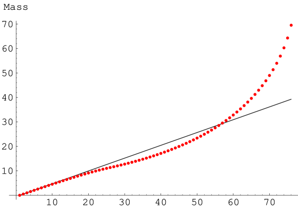
Figure 1: Numerical comparison of the deconstructed KK spectrum (red circles) and the continuum one (black line). KK masses are given in units of $k$. The deconstructed spectrum is calculated for $N=75$ and $q=0.97$, which corresponds to the warp factor $a_{L}\approx 0.102$ on the continuum side.

Summarizing, we see that above the scale $q^{N}gv$, the spectrum depends (approximately) exponentially on $n$, rather than linearly, and resembles nothing one encounters in a 5D theory. It is worthwhile to emphasize that the linear “continuum” regime is not just the linear approximation of the subsequent exponential regime, at least for small $\delta$. In fact, for the first few modes in the exponential regime, the masses grow more slowly than in the linear regime. This can be clearly seen in Fig. 1.

A similar analysis can be applied to study the KK profiles. As we have already mentioned, for KK modes with masses below $gvq^{N}$ they match the continuum ones. Above this scale, the deconstructed KK profiles are still described by continuum Bessel functions for $j<j_{*}$, where $q^{j_{*}}=m_{n}/gv$. However, since the mass of the deconstructed $n$-th mode is different from the continuum one, the deconstructed profile is different as well. The normalization factor is different too, because of the behaviour at large $j$. For $j>j_{*}$, the quantization condition (39) and the asymptotic behaviour of the q-Bessel functions given by eqs. (B.32), (B.34) and (B.41) imply that the deconstructed KK profiles are exponentially damped, in contrast with the continuum ones, which oscillate with increasing amplitude. Hence, above $gvq^{N}$, deconstructed KK modes are decoupled from the IR brane, while they are more strongly coupled than the continuum ones to the UV brane, because of a larger normalization factor. We plot in Fig. 2 a typical deconstructed KK profile in the regime $m_{n}\gg gvq^{N}$, together with its continuum counterpart.

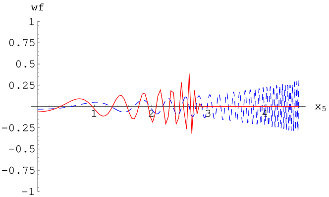
Figure 2: Deconstructed (red continuous line) and continuum (blue dashed line) KK profiles of the mode $n=55$, for $N=100$ and $q=0.955$, which corresponds to the warp factor $a_{L}\approx 0.010$.

The preceding discussion identified the deviation scale

$$\Lambda_{D}=g\,v\,q^{N}\,,$$ (55)

above which the deconstructed KK spectrum and profiles no longer match those of the continuum theory. Using the dictionary (3) the deviation scale is translated to $\Lambda a_{L}=\Lambda(L)$, which is the cutoff scale on the IR brane. Note that for $q\sim 1$ this scale is much larger than the KK scale $M_{KK}\sim\delta gvq^{N}$ and there are $\sim 1/\delta$ KK excitations that are properly matched.

However the applicability range of the continuum theory is far larger, as long as we keep to the appropriate observables. For example, as we discussed above, 5D UV brane physics remains perturbative up to a much higher scale, of order $\Lambda_{S}(0)=1/g_{5}^{2}$. Naively, it would seem that deconstruction cannot reproduce continuum UV brane physics above the scale $\Lambda_{D}$. We will show however that it does.

Consider the deconstructed UV propagator at Euclidean momenta, eq. (48). According to (B.36) and (B.45), the modified q-Bessel functions eq. (48) share the property with their continuum analogues that at large argument $K_{\nu}(x;q^{2})\ll I_{\nu}(x;q^{2})$, including the $x\gg 1$ region where they deviate from the continuum $K$ and $I$ functions. Thus, for $p_{E}\stackrel{{\scriptstyle>}}{{{}_{\sim}}}\delta gvq^{N}$ we can approximate

$$P_{00}(-p_{E}^{2})\approx{ig\over vp_{E}}{K_{1}({p_{E}\over gv};q^{2})\over K_{0}({p_{E}\over gv};q^{2})}\approx{ig\over vp_{E}}{K_{1}({p_{E}\over\delta gv})\over K_{0}({p_{E}\over\delta gv})}\,.$$ (56)

The last equality involving only continuum Bessel functions holds for $p_{E}\stackrel{{\scriptstyle<}}{{{}_{\sim}}}gv$. We can see that $P_{00}$ correctly reproduces the continuum UV propagator (with $k=\delta gv$, $g_{5}^{2}=g/v$) at energies below $gv$, cf. (2.1.2) and (22). This ensures that the two frameworks describe the same UV brane physics (for example, scattering amplitudes of UV brane localized matter fields) below $gv$. The limiting scale is translated to $\Lambda=\Lambda(0)$ – the cutoff scale on the UV brane.

On the other hand, on the IR brane the matching is terminated at a lower scale. For $p_{E}\stackrel{{\scriptstyle>}}{{{}_{\sim}}}gvq^{N}$ the deconstructed propagator is purely four-dimensional, $P_{NN}(-p_{E}^{2})\approx ig^{2}/p_{E}^{2}$, and deviates from the $1/p_{E}$ behaviour of the continuum IR propagator. Thus IR physics is matched by deconstruction only below the scale $gvq^{N}$, which is translated to the cutoff scale on the IR brane $\Lambda(L)$. We compare the continuum and deconstructed UV and IR propagators in Fig. 3.

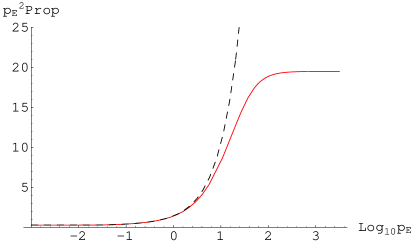
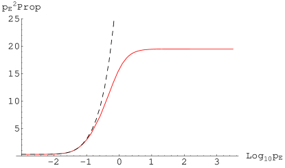
Figure 3: Deconstructed (red continuous line) and continuum (black dashed line) Euclidean brane-to-brane propagators at the UV (left) and IR (right) branes, for $N=70$ and $q=0.95$, and thus $a_{L}\approx 0.0276$. Momenta are given in units of $k$.

This discussion can be easily generalized to show that, for an arbitrary position $y$ in the bulk, deconstruction reproduces continuum physics up to $\Lambda(y)=\Lambda a(y)$. Therefore, the deconstruction framework we consider is indeed a realization of a position-dependent cutoff.

Let us pause for a moment to summarize what we have shown so far. Our results imply that deconstruction provides a correct approximation of the continuum physics at the UV and IR branes, and at any position in the bulk. The matching holds all the way up to the respective position-dependent cutoff scale. In particular, for $\Lambda\sim 1/g_{5}^{2}$ deconstruction works well all the way up to the position-dependent strong-coupling scale, that is in the entire perturbativity range of the continuum theory. The correspondence extends to the energy range where the KK spectra and profiles in the two theories are completely different.

We were able to establish the agreement of the deconstructed and continuum theories in the position approach. However, it all seems miraculous from the point of view of the KK approach. As we have discussed before, the deconstructed KK masses and profiles deviate from the continuum one at the scale $\Lambda_{D}$. Thus, in the two frameworks scattering amplitudes above $\Lambda_{D}$ involve an exchange of a different number of KK modes with different masses and couplings to the brane fields. Somehow, for UV brane amplitudes the two effects cancel and both frameworks predict the same result. The reason for the better agreement of the UV propagators is the locality of the action (28) in the extra-dimensional lattice: the Euclidean UV propagator is screened from the IR brane. On the other hand, the KK masses are determined by global properties of the theory and are thus sensitive to the physics at the IR brane.

Of course, strictly speaking, the matching of the propagators holds only for $t$-channel amplitudes, when the propagators carry space-like momenta. An $s$-channel experiment on the UV brane with enough precision could resolve individual KK resonances, which do not fit in the two theories, and distinguish our completion from a strongly-coupled continuum theory. In this case, above $\Lambda_{D}$, the matching holds only when the energy spread of the scattered beams is sufficiently larger than the KK spacing, so that individual resonances cannot be resolved.

We now move to discussing the situation when the parameter $q$ is not close to $1$, that is when deconstruction is away from the continuum limit. In this case there is no energy regime where the deconstructed spectrum mimics the continuum one. However, earlier works that concentrated on $q\ll 1$ showed that also in this regime deconstruction reproduces certain features of the continuum theory, for example logarithmic running of gauge couplings. We are now in a position to make the relation more precise and interpolate between the different values of $q$.

At the level of the spectrum, for general $q$ we can again distinguish three regimes. For $m_{n}\stackrel{{\scriptstyle<}}{{{}_{\sim}}}q^{N+1}gv$, the spectrum is also linear, but now this regime holds only for a few modes. For $m_{n}\stackrel{{\scriptstyle>}}{{{}_{\sim}}}q^{N+1}gv$, the KK masses are given with great precision by (53), and only the last few modes with $(1-q)gv\stackrel{{\scriptstyle<}}{{{}_{\sim}}}m_{n}\stackrel{{\scriptstyle<}}{{{}_{\sim}}}gv$ deviate; see Fig. 4. In the limit $q\ll 1$ we see that only the exponential regime survives, in agreement with [10, 11, 12]. The behaviour of the KK profiles is qualitatively the same as the one discussed before.

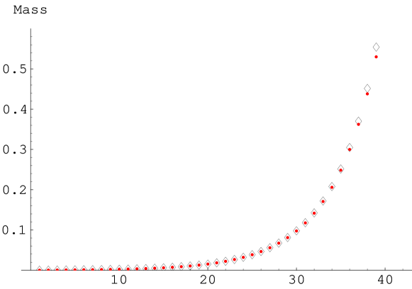
Figure 4: Comparison of our approximate analytical spectrum (black empty diamonds) and the numerical one (red solid circles) for $N=50$ and $q=0.832$, and thus $a_{L}\approx 10^{-4}$, in units $k=1$. We plot only the first 40 modes, which lie in the region of validty of our approximation. The relative error is below 1% for all but the last few modes.

Consider now, once more, the UV propagator (48), but now for arbitrary $q$. At large argument $I$ still dominates over $K$, so that at energies above the KK mass gap, $p_{E}\stackrel{{\scriptstyle>}}{{{}_{\sim}}}gvq^{N+1}$, we can approximate

$$P_{00}(-p_{E}^{2})\approx{ig\over vp_{E}}{K_{1}(p_{E}/gv;q^{2})\over K_{0}(p_{E}/gv;q^{2})}\,.$$ (57)

As long as $p_{E}\stackrel{{\scriptstyle<}}{{{}_{\sim}}}gv$, we can use the small argument asymptotics (Appendix B) of the modified q-Bessel functions to obtain

$$P_{00}(-p_{E}^{2})\approx{1\over\log\left(gv(1-q^{2})e^{-\gamma_{q^{2}}}/q^{1/2}p_{E}\right)}{ig^{2}\log q^{-1}\over p_{E}^{2}}\,.$$ (58)

The deconstructed UV propagator exhibits analogous momentum dependence to that of the continuum UV propagator below the curvature scale, cf. eq. (2.1.2). The factor $g_{5}^{2}k$ in the continuum is replaced here by $g^{2}\log q^{-1}$, in agreement with the dictionary (3). Away from the continuum limit, for $q$ much smaller than $1$, only the argument of the “classical log” does not match the continuum value. Therefore deconstruction with arbitrary $q$ captures the essentials of the continuum UV brane physics below the scale $k$. This explains why deconstruction could reproduce certain features of the 5D theory, such as the logarithmic running of gauge couplings [25], also in the parameter space away from the continuum limit.

This brings us to a comment on the relation of deconstruction and holographic CFTs. We have argued that the UV boundary physics is reproduced in deconstruction for arbitrary $q$, below the scale $gv$ where the approximation (58) is valid. Therefore it is natural to conjecture that deconstructed models, also in the parameters range where they do not have a 5D interpretation, describe the dynamics of some large $N_{c}$ strongly-coupled theories which are approximately conformal over a range of scales. This is an interesting generalization of the AdS/CFT conjecture. In the case at hand 4D strongly-coupled theories might be dual to weakly-coupled 4D theories with extended gauge symmetry. Matching the propagator (58) onto the quark bubble calculation in QCD at large Euclidean momentum, the number of colours in the CFT can be related to the parameters of deconstruction:

$$N_{c}={12\pi^{2}\over g^{2}\log q^{-1}}\,.$$ (59)

According to the dictionary (3) we have $g_{5}^{2}k\longleftrightarrow g^{2}\log q^{-1}$, so this a translation of the well-known AdS/CFT relation $N_{c}=12\pi^{2}/g_{5}^{2}k$.

5 Summary and outlook

In this paper we clarified in what sense and in which parameters range deconstruction approximates 5D gauge theories in the Randall–Sundrum background. In our analysis of the deconstructed theory, we employed powerful tools of the mathematical theory of q-Bessel functions. This allowed us to study analytically the parameter space that was previously accessible only to numerical methods, including the $q\sim 1$ region where the corresponding 5D theory is under control.

The main result of this paper is an explicit proof that a warped 5D gauge theory can be approximated by deconstruction in all its perturbativity range. More precisely, deconstruction provides a faithful description all the way up to the position-dependent cutoff $\Lambda(x_{5})=a(x_{5})\Lambda$, where $\Lambda$ is the inverse lattice spacing. In particular, the continuum theory with $\Lambda\sim 1/g_{5}^{2}$ can be reproduced by deconstructed models with perturbative gauge coupling, $g\sim 1$, in which case the matching extends all the way up to the position-dependent strong-coupling scale $\Lambda_{S}(x_{5})=a(x_{5})/g_{5}^{2}$. This is not a trivial result, as the KK spectra of the two theories deviate at a much lower scale, $\Lambda_{D}=a_{L}\Lambda$.

The technical results we derived can be readily applied to more phenomenological studies. In fact, we have shown that computations in deconstructed warped theories can be performed at the quantitative level comparable to that in 5D. This is an encouragement to study deconstructed versions of phenomenological models in ${\mathrm{A}\mathrm{d}\mathrm{S}}_{5}$, such as the models of the electroweak sector of refs. [2]. Deconstruction could provide for a UV completion of these models that could remain perturbative to much higher energy scales. Furthermore, deconstruction offers a playground to study the evolution of gauge couplings in ${\mathrm{A}\mathrm{d}\mathrm{S}}_{5}$ [25, 17]. This was already exploited in [10, 11], but only in the region $q\ll 1$, where the link with the 5D computation is obscure. The virtue of deconstruction in this case it that it provides a concrete physical realization of the 5D cutoff physics, which allows, in particular, to study threshold effects.

It would also be interesting to exploit the relation of deconstruction with holographic CFTs. Most interestingly, deconstruction can describe certain aspects of the real-world QCD in the strongly coupled regime. For example, chiral symmetry breaking and physics of $\rho$ and $a$ resonances can be captured, as shown in ref. [26]. More recently, effective description of low energy QCD was pursued in 5D continuum models [7]. Our results allow for quantitative studies of deconstructed versions of these models. This could shed further light on the origin of this AdS/QCD correspondence and its connection to the Migdal’s approach [27] discussed recently in [28]. Indeed, the high energy behaviour of the continuum correlation functions, which is non-analytic in $p^{2}$, is approximated in deconstruction by a ratio of polynomials, similarly as in the Migdal’s approach.

Finally, we note that the methods used here can be directly applied to fields with different spins, at least in the massless case. For instance, the difference equation for the graviton corresponds to the Hahn–Exton equation (B.1) with $\nu=2$. Therefore, all the results presented here for gauge bosons translate in a straightforward way to the gravity case. In particular, the qualitative features of the spectrum are the same, and agree with the discussion presented in ref. [15]. It is also likely that the methods of q-difference equations can be applied to study deconstruction of more general backgrounds than the Randall–Sundrum ${\mathrm{A}\mathrm{d}\mathrm{S}}_{5}$ one.

Appendix A Implementation of general boundary conditions

We generalize our results to gauge theories with Dirichlet boundary conditions on one or on both branes.

The mixed momentum–position space propagator for a gauge boson in a slice of ${\mathrm{A}\mathrm{d}\mathrm{S}}_{5}$ can be succinctly written as

$$P^{\alpha\beta}(p^{2},x_{5},y_{5})={i\pi g_{5}^{2}\over 2k}{\left(A^{\alpha}[0]J_{1}({p\over ka(x_{5})})-B^{\alpha}[0]Y_{1}({p\over ka(x_{5})})\right)\left(A^{\beta}[L]J_{1}({p\over ka(y_{5})})-B^{\beta}[L]Y_{1}({p\over ka(y_{5})})\right)\over a(x_{5})a(y_{5})\left(A^{\alpha}[0]B^{\beta}[L]-B^{\alpha}[0]A^{\beta}[L]\right)}\,,$$ (A.1)

where the parameters $A^{\alpha}[0]$, $B^{\alpha}[0]$, $A^{\beta}[L]$, $B^{\beta}[L]$ depend on the boundary conditions. They take the values

$$A^{N}[x_{5}]=Y_{0}\left({p\over ka(x_{5})}\right)\,,\qquad\qquad B^{N}[x_{5}]=J_{0}\left({p\over ka(x_{5})}\right)$$ (A.2)

if Neumann boundary conditions are imposed at $x_{5}$, and

$$A^{D}[x_{5}]=Y_{1}\left({p\over ka(x_{5})}\right)\,,\qquad\qquad B^{D}[x_{5}]=J_{1}\left({p\over ka(x_{5})}\right)$$ (A.3)

for Dirichlet boundary conditions at $x_{5}$. We can also define brane-to-brane propagators, as long as we deal with Neumann boundary conditions on the given brane. For example, for the Neumann–Dirichlet case we obtain the UV brane-to-brane propagator

$$P_{\mathrm{U}V}^{\mathrm{N}D}(p^{2})\equiv P^{\mathrm{N}D}(p^{2},0,0)={ig_{5}^{2}\over p}{Y_{1}({p\over ka_{L}})J_{1}({p\over k})-J_{1}({p\over ka_{L}})Y_{1}({p\over k})\over Y_{0}({p\over k})J_{1}({p\over ka_{L}})-J_{0}({p\over k})Y_{1}({p\over ka_{L}})}\,,$$ (A.4)

which is suppressed for $\sqrt{-p^{2}}\ll M_{\mathrm{K}K}$, while for $\sqrt{-p^{2}}\gg M_{\mathrm{K}K}$ it is indistinguishable from the UV propagator in the Neumann–Neumann case.

We turn to discussing the method of realizing these more general boundary conditions in deconstruction. To this end we include two more scalar fields: $\Phi_{0}$ charged under $A_{\mu}^{0}$ with a vev $v_{0}/\sqrt{2}$ and $\Phi_{N+1}$ charged under $A_{\mu}^{N}$ with a vev $v_{N+1}/\sqrt{2}$, so that the boundary entries in the gauge boson mass matrix are modified. The effect of the additional vev’s is to modify the “boundary conditions” for the propagator. More precisely, eq. (42) represents the correct propagator equation if we impose

$$P_{-1,k} = {v^{2}-v_{0}^{2}\over v^{2}}P_{0,k}\,,$$

$$P_{N+1,k} = {v^{2}-q^{-2(N+1)}v_{N+1}^{2}\over v^{2}}P_{N,k}\,.$$ (A.5)

Setting $v_{0}=v_{N+1}=0$ we recover the Neumann boundary conditions (43). With $v_{0}=v$ we get $P_{-1,k}=0$ which mimics the Dirichlet boundary conditions on the UV brane. Similarly $v_{N+1}=q^{N+1}v$ yields $P_{N+1,k}=0$, which is a deconstructed version of the Dirichlet boundary conditions on the IR brane. Other choices of $v_{0}$ and $v_{N+1}$ correspond to mixed boundary conditions on the continuum side.

We are now in a position to write the general form of the deconstructed position propagator:

$$\displaystyle P_{jk}^{\alpha\beta}(p^{2})={i\pi\over v^{2}(1-q^{2})}q^{-k-j}$$

$$\displaystyle{[A^{\alpha}[0]J_{1}({q^{-j}x};q^{2})-B^{\alpha}[0]Y_{1}({q^{-j}x};q^{2})][A^{\beta}[L]J_{1}({q^{-k}x};q^{2})-B^{\beta}[L]Y_{1}({q^{-k}x};q^{2})]\over A^{\alpha}[0]B^{\beta}[L]-B^{\alpha}[0]A^{\beta}[L]}\,.$$

Neumann (N) or Dirichlet (D) boundary conditions specify the parameters in eq. (Appendix A) as follows

$$\displaystyle A^{\mathrm{N}}[0]=Y_{0}(x;q^{2})\qquad\qquad B^{\mathrm{N}}[0]=J_{0}(x;q^{2})$$

$$\displaystyle A^{\mathrm{N}}[L]=Y_{0}(q^{-N-1}x;q^{2})\qquad\qquad B^{\mathrm{N}}[L]=J_{0}(q^{-N-1}x;q^{2})$$

$$\displaystyle A^{\mathrm{D}}[0]=Y_{1}(qx;q^{2})\qquad\qquad B^{\mathrm{D}}[0]=J_{1}(qx;q^{2})$$

$$\displaystyle A^{\mathrm{D}}[L]=Y_{1}(q^{-N-1}x;q^{2})\qquad\qquad B^{\mathrm{D}}[L]=J_{1}(q^{-N-1}x;q^{2})\,.$$ (A.7)

The correspondence between eqs. (A.1) and (Appendix A) can be established using the methods discussed in Section 4. In particular, below the deviation scale $\Lambda_{D}=gvq^{N}$ (translated to the IR cutoff scale $\Lambda(L)=a_{L}\Lambda$), physical amplitudes in deconstruction mimic those in the continuum theories at the leading order in $\delta$ and $p/gv$. Above the deviation scale, the spectra (the poles of the propagator) are different. However $t$-channel amplitudes on the UV brane are still reproduced in deconstruction, all the way to the UV cutoff $\Lambda(0)=\Lambda$. Therefore for general boundary conditions the correspondence between deconstruction and continuum holds at the same quantitative level as for the Neumann–Neumann case discussed in Sections 3 and 4.

Appendix B Q-tutorial

This appendix contains definitions of the q-Bessel functions and a review of their vital properties. Our presentation is based mainly on ref. [21]. We also derive several results concerning the asymptotic behaviour of the q-Bessel functions, which have not been given in the literature.

Several inequivalent q-analogues of the Bessel functions have been studied in the mathematical literature. The ones relevant to our purpose are solutions of the so-called Hahn–Exton q-difference equation,

$$(q^{\nu/2}+q^{-\nu/2}-q^{-\nu/2}t^{2})F(t)-F(tq^{-1/2})-F(tq^{1/2})=0\,.$$ (B.1)

For definiteness we consider $0<q<1$. One solution of this equation is the Hahn-Exton q-Bessel function [20] (q-Bessel in the following) denoted by $J_{\nu}(t;q)$. It is defined by the power series

$$J_{\nu}(t;q)=t^{\nu}{(q^{\nu+1};q)_{\infty}\over(q;q)_{\infty}}\sum_{k=0}^{\infty}{(-1)^{k}q^{k(k+1)/2}\over(q^{\nu+1};q)_{k}(q;q)_{k}}t^{2k}\,,$$ (B.2)

where the q-shifted factorials are defined as

$$(a;q)_{k}=\left\{\begin{array}[]{ll}1&\mbox{if $k=0$}\\ \prod_{n=0}^{k-1}(1-aq^{n})&\mbox{if $k\geq 1$}\end{array}\right.\,$$ (B.3)

for $a\in\mathbb{C}$ and $k\in\mathbb{Z}_{+}\equiv\{0,1,2,\ldots\}$, and $(a;q)_{\infty}=\lim_{k\rightarrow\infty}(a;q)_{k}$. The q-Bessel $J_{\nu}(.;q)$ is analytic in $\mathbb{C}\backslash\{0\}$. For $\nu=n\in\mathbb{Z}$ and $|t|<1$, it has an integral representation:

$$J_{n}(t;q)={1\over 2\pi}\int_{0}^{2\pi}{(qte^{-i\phi};q)_{\infty}\over(te^{i\phi};q)_{\infty}}e^{-in\phi}\,.$$ (B.4)

It is known that all the zeros of the q-Bessel function of order $\nu>-1$ are real and that the non-zero ones are simple [22].

For $\nu\notin{\bf Z}$ $J_{\nu}(t;q)$ and $J_{-\nu}(tq^{-\nu/2};q)$ are two independent solutions of eq. (B.1); however, for integer $\nu=n$, there is the relation $J_{-n}(t;q)=(-1)^{n}q^{\frac{n}{2}}J_{n}(tq^{\frac{n}{2}};q)$. Therefore one introduces the q-Neumann function $Y_{\nu}(t;q)$, which is an independent solution for arbitrary $\nu$:

$$Y_{\nu}(t;q)={\Gamma_{q}(\nu)\Gamma_{q}(1-\nu)\over\pi}\,q^{-\frac{\nu^{2}}{2}}\,\left[\cos(\pi\nu)q^{\nu\over 2}J_{\nu}(t;q)-J_{-\nu}(tq^{-\frac{\nu}{2}};q)\right]\,,$$ (B.5)

where

$$\Gamma_{q}(\nu)={(q;q)_{\infty}\over(q^{\nu};q)_{\infty}}(1-q)^{1-\nu}$$ (B.6)

is a q-extension of the Euler $\Gamma$-function, satisfying $\lim_{q\to 1^{-}}\Gamma_{q}(\nu)=\Gamma(\nu)$. For integer $\nu$, the limit $\nu\to n\in{\mathbb{Z}}$ is understood on the r.h.s. of eq. (B.5). Explicitly, this limit gives [23]

$$Y_{n}(t;q)= \frac{2(q-1)}{\pi\log q}J_{n}(t;q)\log\frac{t}{1-q}$$

$$\mbox{}-\frac{1-q}{\pi}t^{-n}\sum_{k=0}^{n-1}\frac{(q;q)_{n-k-1}t^{2k}}{(q;q)_{k}}$$

$$\mbox{}+\frac{1-q}{\pi\log q}t^{n}\sum_{k=0}^{\infty}\frac{(-1)^{k}q^{k(k+1)\over 2}t^{2k}}{(q;q)_{k}(q;q)_{n+k}}\left\{\frac{\Gamma^{\prime}_{q}(n+k+1)}{\Gamma_{q}(n+k+1)}+\frac{\Gamma^{\prime}_{q}(k+1)}{\Gamma_{q}(k+1)}\right\}$$

$$\mbox{}-\frac{1-q}{2\pi}t^{n}\sum_{k=0}^{\infty}\frac{(-1)^{k}q^{k(k+1)/2}t^{2k}(2k+1)}{(q;q)_{k}(q;q)_{n+k}}\,$$ (B.7)

for $n\in\mathbb{Z}_{+}$ (omitting the second term when $n=0$). For negative integers $Y_{-n}(t;q)=(-1)^{n}q^{\frac{n}{2}}Y_{n}(tq^{\frac{n}{2}};q)$.

We now review properties of the q-Bessel and q-Neumann functions. Since the form relevant to deconstruction is $J_{\nu}(t;q^{2})$ and $Y_{\nu}(t;q^{2})$ (rather than $J_{\nu}(t;q)$ and $Y_{\nu}(t;q)$), we find it convenient to present all formulas in this form.

The q-Bessels and q-Neumanns are q-analogues of the ordinary Bessel and Neumann functions, in the sense that there exists the “continuum limit” $q\to 1$,

$$\lim_{q\rightarrow 1^{-}}Z_{\nu}\left((1-q)t;q^{2}\right)=Z_{\nu}(t)\,,$$ (B.8)

with $Z=J,Y$ and $J_{\nu}(.),Y_{\nu}(.)$ the ordinary Bessel and Neumann functions. For $q$ close to $1$, the continuum approximation holds for $(1-q)|t|\ll 1$, as can be seen from both the series and the integral representations. In fact, when $q=1-{\delta}\sim 1$ and $|t|\ll 1$, we can Taylor expand $F(q^{\pm 1}t)$ in powers of $({\delta}t)$. Keeping terms up to the second derivative, we obtain

$${\delta}^{2}t^{2}F^{\prime\prime}(t)+{\delta}^{2}tF^{\prime}(t)+(q^{-\nu}t^{2}-q^{\nu}-q^{-\nu})F(t)=0\,,$$ (B.9)

which is solved by the Bessel or Neumann functions:

$$F(t)=Z_{4\sinh^{2}[\log q\nu/2]}\left({t\over q^{\nu}{\delta}}\right)\approx Z_{\nu}\left({t\over{\delta}}\right)\,.$$ (B.10)

This derivation is valid as long as higher derivatives in the Taylor expansion of $F(q^{\pm 1}t)$ can be neglected, that is when $|{\delta}tF^{\prime\prime\prime}(t)|\ll|F^{\prime\prime}(t)|$. For the solution eq. (B.10) this is indeed true for $|t|\ll 1$.

The q-Bessels and q-Neumann satisfy recursion relations analogous to the ones of their continuous cousins. In particular, the following ones will prove very useful

$$q^{\nu}Z_{\nu}(t;q^{2})-Z_{\nu}(qt;q^{2})=-qtZ_{\nu+1}(qt;q^{2})\,,$$

$$Z_{\nu}(t;q^{2})-q^{\nu}Z_{\nu}(qt;q^{2})=tZ_{\nu-1}(t;q^{2})\,,$$ (B.11)

with $Z=J,Y$. These are actually discrete versions of difference–recurrence relations. Indeed, one can define the q-derivative of a function as

$$D_{q}f(t)=\left\{\begin{array}[]{ll}\frac{f(t)-f(tq)}{t(1-q)}&~{}\mbox{if}~{}t\neq 0\\ f^{\prime}(0)&~{}\mbox{if}~{}t=0\end{array}\right.\,,$$ (B.12)

which is a q-analogue of the continuum derivative: $\lim_{q\rightarrow 1^{-}}D_{q}f(t)=f^{\prime}(t)$. Then, (Appendix B) are a particular case ($k=1$) of [21]:

$$\left[t^{-1}D_{q}\right]^{k}\left[t^{-\nu}Z_{\nu}(t;q^{2})\right]=\frac{(-1)^{k}t^{-\nu-k}q^{k(1-\nu)}}{\left(1-q\right)^{k}}Z_{\nu+k}(tq^{k};q^{2})$$

$$\left[t^{-1}D_{q}\right]^{k}\left[t^{\nu}Z_{\nu}(t;q^{2})\right]=\frac{t^{\nu-k}}{\left(1-q\right)^{k}}Z_{\nu-k}(t;q^{2})\,.$$ (B.13)

For $q\to 1$ this reduces to the familiar recursion relations of the continuum Bessel functions.

The Wronskian of a differential equation has also its q-analogue. In general for a q-difference equation of the form $F(qt)+F(q^{-1}t)+P(t,q)F(t)=0$, its two independent $F_{1}(t)$ and $F_{2}(t)$ solutions satisfy the relation $F_{1}(qt)F_{2}(t)-F_{1}(t)F_{2}(qt)=C(q)$ with the r.h.s. independent of $t$. For q-Bessels, the q-Wronskian relation is

$$J_{\nu}(qt;q^{2})Y_{\nu}(t;q^{2})-Y_{\nu}(qt;q^{2})J_{\nu}(t;q^{2})={q^{-\nu}(1-q^{2})\over\pi}\,,$$ (B.14)

which can be proved using the series expansion of the q-Bessels. The fact that the q-Wronskian does not vanish at any point $t$ implies that a general solution of the q-difference equation (B.1) can be written as [23]

$$F(t)=A(t)J_{\nu}(t;q^{2})+B(t)Y_{\nu}(t;q^{2})\,,$$ (B.15)

where $A(t)$ and $B(t)$ are q-periodic, i.e. they satisfy $A(qt)=A(t)$, $B(qt)=B(t)$. But since we are interested only in discrete values of the argument, $t_{0},qt_{0},q^{2}t_{0},\ldots$, we can simply treat $A$ and $B$ as constants.

We can also define q-analogues of the modified Bessel and Bessel–Macdonald functions, which are solutions of the Euclidean version of the q-difference equation (B.1),

$$(q^{\nu/2}+q^{-\nu/2}+q^{-\nu/2}t^{2})F(t)-F(tq^{-1/2})-F(tq^{1/2})=0\,.$$ (B.16)

We define the q-modified-Bessel as

$$I_{\nu}(t;q)=i^{-\nu}J_{\nu}(it;q)\,,$$ (B.17)

and the q-Bessel–Macdonald as

$$K_{\nu}(t;q)=\frac{1}{2}q^{-{\nu^{2}\over 2}}\Gamma_{q}(\nu)\Gamma_{q}(1-\nu)\left[I_{-\nu}(q^{-{\nu\over 2}}t;q)-q^{\nu\over 2}I_{\nu}(t;q)\right]\,,$$ (B.18)

with a limit understood for integer $\nu$. Our definitions agree with the ones in [24], up to a change of variables and a global factor. Equivalently, we can write

$$K_{\nu}(t;q)=\frac{\pi}{2}i^{\nu+1}\left[\frac{\Gamma_{q}(\nu)\Gamma_{q}(1-\nu)}{\pi}\sin\nu\pi q^{\frac{1}{2}\nu(1-\nu)}J_{\nu}(it;q)+iY_{\nu}(it;q)\right]\,.$$ (B.19)

Taking the limit of integer index, we find

$$K_{n}(t;q)=\frac{\pi}{2}i^{n+1}\left[\frac{(-1)^{n}(1-q)(q;q)_{n-1}}{\log q(q^{1-n};q)_{n-1}}q^{\frac{1}{2}n(1-n)}J_{n}(it;q)+iY_{n}(it;q)\right]\,,$$ (B.20)

for $n\in\mathbb{N}$ and

$$K_{0}(t;q)=\frac{\pi}{2}i\left[\frac{(1-q)}{-\log q}J_{0}(it;q)+iY_{0}(it;q)\right]\,.$$ (B.21)

The continuum limit is

$$\lim_{q\rightarrow 1^{-}}X_{\nu}\left((1-q)t;q^{2}\right)=X_{\nu}(t)\,,$$ (B.22)

with $X=I,K$. The q-modified-Bessels and the q-Bessel–Macdonalds satisfy the recurrence relations

$$\left[t^{-1}D_{q}\right]^{k}\left[t^{-\nu}X_{\nu}(t;q^{2})\right]=\frac{(-1)^{\alpha k}t^{-\nu-k}q^{k(1-\nu)}}{\left(1-q\right)^{k}}X_{\nu+k}(tq^{k};q^{2})$$

$$\left[t^{-1}D_{q}\right]^{k}\left[t^{\nu}X_{\nu}(t;q^{2})\right]=(-1)^{\alpha k}\frac{t^{\nu-k}}{\left(1-q\right)^{k}}X_{\nu-k}(t;q^{2})\,,$$ (B.23)

with $\alpha=0,1$ for $X=I,K$, respectively. The q-Wronskian is

$$I_{\nu}(qt;q^{2})K_{\nu}(t;q^{2})-K_{\nu}(qt;q^{2})I_{\nu}(t;q^{2})=-{q^{-\nu}(1-q^{2})\over 2}\,,$$ (B.24)

and a general solution of (B.16) can be written as

$$F(t)=A(t)I_{\nu}(t;q^{2})+B(t)K_{\nu}(t;q^{2})\,,$$ (B.25)

with $A,B$ q-periodic functions, which again we can consider constant.

The behaviour of all these functions at small values of the argument can be read from the corresponding series expansions. We list below the small-argument asymptotics that are useful for our computations

$$J_{0}(t;q^{2})\approx I_{0}(t;q^{2})\approx 1\,,$$

$$J_{1}(t;q^{2})\approx I_{1}(t;q^{2})\approx\frac{t}{1-q^{2}}\,,$$

$$Y_{0}(t;q^{2})\approx\frac{1-q^{2}}{-\pi\log q}\left(\log\frac{q^{\frac{1}{2}}t}{1-q^{2}}+\gamma_{q^{2}}\right)\,,$$

$$Y_{1}(t;q^{2})\approx-\frac{1-q^{2}}{\pi}t^{-1}\,,$$

$$K_{0}(t;q^{2})\approx\frac{1-q^{2}}{2\log q}\left(\log\frac{q^{\frac{1}{2}}t}{1-q^{2}}+\gamma_{q^{2}}\right)\,,$$

$$K_{1}(t;q^{2})\approx\frac{1-q^{2}}{2}t^{-1}\,,$$

for $|t|\ll 1$. We have defined the q-Euler–Mascheroni constant $\gamma_{q}=-\Gamma^{\prime}_{q}(1)$. Its series representation is

$$\gamma_{q^{2}}=\log(1-q^{2})-\log q^{2}\sum_{k=1}^{\infty}\frac{q^{2k}}{1-q^{2k}}\,.$$ (B.27)

Varying $q$ from 0 to 1, $\gamma_{q^{2}}$ grows approximately linearly from 0 to $\gamma=0.577\ldots$.

Obtaining the asymptotic behaviour at large argument is more involved. We first look at the asymptotic form of the Hahn–Exton equation (B.1). Writing $F(t)=\Pi(t)G(t)$, where

$$\Pi(t)=\prod_{k=1}^{\infty}(1-q^{2k}t^{2})\equiv(q^{2}t^{2};q^{2})_{\infty}\,$$ (B.28)

and using $\Pi(qt)=\Pi(t)/(1-q^{2}t^{2})$, $\Pi(q^{-1}t)=\Pi(t)(1-t^{2})$ the Hahn–Exton equation takes the form

$$G(qt)+(1-t^{2})(1-q^{2}t^{2})G(q^{-1}t)+(1-q^{2}t^{2})(t^{2}q^{-\nu}-q^{\nu}-q^{-\nu})G(t)=0\,,$$ (B.29)

which for $|t|\gg 1$ reduces to

$$G(qt)+q^{2}t^{4}G(q^{-1}t)-q^{2}t^{4}q^{-\nu}G(t)=0\,.$$ (B.30)

One solution follows from neglecting the first term: $G(t)={\rm const}\ t^{\nu}$. From eq. (B.30) we see that this approximation should work fine very quickly when $|t|$ becomes larger than $1$. To find the second solution it is more convenient to insert $F(t)=(1/\Pi(t))G(t)$ in eq. (B.1), which leads to the equation

$$G(qt)(1-t^{2})(1-q^{2}t^{2})+G(q^{-1}t)+(1-t^{2})(t^{2}q^{-\nu}-q^{\nu}-q^{-\nu})G(t)=0\,,$$ (B.31)

approximated by $G(qt)=q^{-\nu-2}G(t)=0$ at large $|t|$. The solution is $G(t)={\rm const}\ t^{-\nu-2}$. Therefore, a general solution to the Hahn–Exton equation has the asymptotic form

$$F(t)\approx At^{\nu}(q^{2}t^{2};q^{2})_{\infty}+B{t^{-\nu-2}\over(q^{2}t^{2};q^{2})_{\infty}}\,,\quad\qquad|t|\gg 1\,.$$ (B.32)

For imaginary $t$ one solution grows rapidly (faster than any power of $t$) while the other decays (equally rapidly). For real $t$ the situation is more complicated as the “decaying part” has poles at $t_{n}=q^{-n}$. In the following we pinpoint the coefficient $A$ for the q-Bessel functions defined previously.

We can obtain the asymptotic behaviour of the q-Bessel by approximating $(q^{\nu+1};q)_{k}\approx(q^{\nu+1};q)_{\infty}$ in the power series (B.2). This is justified because for $t\gg 1$ the series is dominated by terms with large $k$ for which this approximation is fine. Using then the so-called q-binomial theorem (see for instance the second reference in [20]),

$$(-t^{2};q^{2})_{\infty}=\sum_{n=0}^{\infty}\frac{q^{n(n-1)}t^{2n}}{(q^{2};q^{2})_{n}}\,,$$ (B.33)

we arrive at

$$J_{\nu}(t;q^{2})\approx t^{\nu}\frac{(q^{2}t^{2};q^{2})_{\infty}}{(q^{2};q^{2})_{\infty}}\,,~{}~{}|t|\gg 1\,.$$ (B.34)

This fixes the normalization of the growing part of the q-Bessel. From this expression we can directly read the asymptotic zeros of the q-Bessel $J_{\nu}(t;q^{2})$, which are located at

$$t_{r}\approx q^{-r}\,,~{}~{}r\in\mathbb{N}\,,~{}~{}q^{-r}\gg 1\,,$$ (B.35)

independently of the index $\nu$ (though, in fact, the approximation (B.34) is better for larger values of $\nu$). Since the above derivation is valid for any argument of $t$, we also find

$$I_{\nu}(t;q^{2})\approx t^{\nu}\frac{(-q^{2}t^{2};q^{2})_{\infty}}{(q^{2};q^{2})_{\infty}}\,,~{}~{}|t|\gg 1\,.$$ (B.36)

Finding the asymptotic form of the q-Neumann is even more involved. For integer index $n\in\mathbb{Z}_{+}$, using (B.5) and (B.34) we have

$$Y_{n}(t;q^{2}) \approx\frac{(-1)^{n}(1-q^{2})(q^{2};q^{2})_{n-1}}{2\pi\log q(q^{2};q^{2})_{\infty}(q^{2-2n};q^{2})_{n-1}}\left[q^{n(1-n)}\log(qt)t^{n}(q^{2}t^{2};q^{2})_{\infty}\phantom{\sum_{r=1}^{\infty}}\right.$$

$$\left.\mbox{}-(-1)^{n}\left(\log\left(\frac{q^{2n}}{t}\right)+2\log q\sum_{r=1}^{\infty}\frac{t^{2}q^{2(r-n)}}{1-q^{2(r-n)}t^{2}}\right)t^{-n}(q^{2-2n}t^{2};q^{2})_{\infty}\right]\,,~{}|t|\gg 1\,,$$ (B.37)

for $n\in\mathbb{N}$,

$$Y_{0}(t;q^{2})\approx\frac{(1-q^{2})}{\pi\log q^{-1}(q^{2};q^{2})_{\infty}}\left[\log t+\log q\left(\frac{1}{2}-\sum_{r=1}^{\infty}\frac{t^{2}q^{2r}}{1-q^{2r}t^{2}}\right)\right](q^{2}t^{2};q^{2})_{\infty}\,,~{}~{}|t|\gg 1\,.$$ (B.38)

Note that the poles in the sum cancel against zeros in $(q^{2-2n}t^{2};q^{2})_{\infty}$. For real $t$, writing $t=q^{-s+\alpha}$, with $s\in\mathbb{N}$ and $\alpha\in]-1/2,1/2]$, and assuming $|\alpha|\ll 1$, we can approximate the sum at large $t$ by

$$\sum_{r=1}^{\infty}\frac{t^{2}q^{2(r-n)}}{1-q^{2(r-n)}t^{2}}=\frac{\log t}{\log q}+1-n+\frac{1}{q^{-2\alpha}-1}+\mathcal{O}\left(t^{-2}\right)\,.$$ (B.39)

Therefore,

$$Y_{n}(t;q^{2}) \approx\frac{(-1)^{n}(1-q^{2})(q^{2};q^{2})_{n-1}}{2\pi\log q(q^{2};q^{2})_{\infty}(q^{2-2n};q^{2})_{n-1}}\left[q^{n(1-n)}\log(qt)t^{n}(q^{2}t^{2};q^{2})_{\infty}\phantom{\frac{1}{q^{-2\alpha}-1}}\right.$$

$$\left.\mbox{}-(-1)^{n}\left(\log t+2\left(1+\frac{1}{q^{-2\alpha}-1}\right)\log q\right)t^{-n}(q^{2-2n}t^{2};q^{2})_{\infty}\right],\,|\alpha|\ll 1,\,t\gg 1\,,$$ (B.40)

for $n\in\mathbb{N}$, and

$$Y_{0}(t;q^{2})\approx\frac{(1-q^{2})}{\pi(q^{2};q^{2})_{\infty}}\left(\frac{1}{2}+\frac{1}{q^{-2\alpha}-1}\right)(q^{2}t^{2};q^{2})_{\infty}\,,~{}~{}|\alpha|\ll 1\,,~{}t\gg 1\,.$$ (B.41)

The corresponding expressions for imaginary argument $t=i\tau$, $\tau\in\mathbb{R}$, are simpler. In this case we can evaluate the relevant sum to leading order at large $|\tau|$ without any further restriction:

$$-\sum_{r=1}^{\infty}\frac{\tau^{2}q^{2(r-n)}}{1+q^{2(r-n)}\tau^{2}}=\frac{\log\tau^{2}}{2\log q}-n+\frac{1}{2}+\mathcal{O}\left(\tau^{-2}\right)\,,$$ (B.42)

which leads to the asymptotics

$$Y_{n}(it;q^{2})\approx i\frac{(-1)^{n}(1-q^{2})(q^{2};q^{2})_{n-1}q^{n(1-n)}}{2\log q(q^{2};q^{2})_{\infty}(q^{2-2n};q^{2})_{n-1}}(it)^{n}(-q^{2}t^{2};q^{2})_{\infty}\,,~{}~{}t\in\mathbb{R}\,,~{}~{}|t|\gg 1\,,$$ (B.43)

for $n\in\mathbb{N}$ and

$$Y_{0}(it;q^{2})\approx i\frac{(1-q^{2})}{2\log q^{-1}(q^{2};q^{2})_{\infty}}(-q^{2}t^{2};q^{2})_{\infty}\,,~{}~{}t\in\mathbb{R}\,,~{}~{}|t|\gg 1\,.$$ (B.44)

This allows us to build a linear combination of the q-Bessel and q-Neumann, which is purely decaying at large imaginary values of the argument. In fact, from the above expression we see that this combination is proportional to the q-Bessel–Macdonald. In other words,

$$K_{n}(t;q)\ll 1\,,~{}~{}t\in\mathbb{R}\,,~{}~{}t\gg 1\,.$$ (B.45)

Therefore, the q-Bessel–Macdonald shares with its continuum counterpart the property that, at large real argument $t$, it is damped. This is true in the “continuum” region as well as for $t\gg 1$ where the continuum approximation fails. We also see that in this regime $K_{n}(t;q)\ll I_{n}(t;q)$. It is plausible that the same behaviour holds for non-integer indices, though we have not proved this result.

References

• [1] L. Randall and R. Sundrum, Phys. Rev. Lett.  83 (1999) 3370 [arXiv:hep-ph/9905221].
• [2] R. Contino, Y. Nomura and A. Pomarol, Nucl. Phys. B 671 (2003) 148 [arXiv:hep-ph/0306259]. K. y. Oda and A. Weiler, Phys. Lett. B 606 (2005) 408 [arXiv:hep-ph/0410061]. K. Agashe, R. Contino and A. Pomarol, Nucl. Phys. B 719 (2005) 165 [arXiv:hep-ph/0412089]. Y. Hosotani and M. Mabe, Phys. Lett. B 615 (2005) 257 [arXiv:hep-ph/0503020]. Y. Hosotani, S. Noda, Y. Sakamura and S. Shimasaki, arXiv:hep-ph/0601241.
• [3] C. Csaki, C. Grojean, L. Pilo and J. Terning, Phys. Rev. Lett.  92 (2004) 101802 [arXiv:hep-ph/0308038]. G. Burdman and Y. Nomura, Phys. Rev. D 69 (2004) 115013 [arXiv:hep-ph/0312247].
• [4] Z. Chacko, Y. Nomura and D. Tucker-Smith, Nucl. Phys. B 725 (2005) 207 [arXiv:hep-ph/0504095].
• [5] J. M. Maldacena, Adv. Theor. Math. Phys.  2 (1998) 231 [Int. J. Theor. Phys.  38 (1999) 1113] [arXiv:hep-th/9711200]. S. S. Gubser, I. R. Klebanov and A. M. Polyakov, Phys. Lett. B 428 (1998) 105 [arXiv:hep-th/9802109]. E. Witten, Adv. Theor. Math. Phys.  2 (1998) 253 [arXiv:hep-th/9802150]. O. Aharony, S. S. Gubser, J. M. Maldacena, H. Ooguri and Y. Oz, Phys. Rept.  323 (2000) 183 [arXiv:hep-th/9905111].
• [6] N. Arkani-Hamed, M. Porrati and L. Randall, JHEP 0108 (2001) 017 [arXiv:hep-th/0012148]. R. Rattazzi and A. Zaffaroni, JHEP 0104 (2001) 021 [arXiv:hep-th/0012248]. M. Pérez-Victoria, JHEP 0105 (2001) 064 [arXiv:hep-th/0105048]. For a recent review, see T. Gherghetta, arXiv:hep-ph/0601213.
• [7] J. Erlich, E. Katz, D. T. Son and M. A. Stephanov, Phys. Rev. Lett.  95 (2005) 261602 [arXiv:hep-ph/0501128]. L. Da Rold and A. Pomarol, Nucl. Phys. B 721 (2005) 79 [arXiv:hep-ph/0501218]. J. Hirn and V. Sanz, JHEP 0512 (2005) 030 [arXiv:hep-ph/0507049]. K. Ghoroku, N. Maru, M. Tachibana and M. Yahiro, Phys. Lett. B 633 (2006) 602 [arXiv:hep-ph/0510334]. J. Hirn, N. Rius and V. Sanz, Phys. Rev. D 73 (2006) 085005 [arXiv:hep-ph/0512240].
• [8] N. Arkani-Hamed, A. G. Cohen and H. Georgi, Phys. Rev. Lett.  86 (2001) 4757 [arXiv:hep-th/0104005]. C. T. Hill, S. Pokorski and J. Wang, Phys. Rev. D 64 (2001) 105005 [arXiv:hep-th/0104035].
• [9] H. Abe, T. Kobayashi, N. Maru and K. Yoshioka, Phys. Rev. D 67 (2003) 045019 [arXiv:hep-ph/0205344].
• [10] A. Falkowski and H. D. Kim, JHEP 0208 (2002) 052 [arXiv:hep-ph/0208058].
• [11] L. Randall, Y. Shadmi and N. Weiner, JHEP 0301 (2003) 055 [arXiv:hep-th/0208120].
• [12] A. Katz and Y. Shadmi, JHEP 0411 (2004) 060 [arXiv:hep-th/0409223].
• [13] C. D. Carone, J. Erlich and B. Glover, arXiv:hep-ph/0509002.
• [14] N. Arkani-Hamed, H. Georgi and M. D. Schwartz, Annals Phys.  305 (2003) 96 [arXiv:hep-th/0210184].
• [15] L. Randall, M. D. Schwartz and S. Thambyapillai, arXiv:hep-th/0507102. J. Gallicchio and I. Yavin, arXiv:hep-th/0507105.
• [16] A. Pomarol, Phys. Lett. B 486 (2000) 153 [arXiv:hep-ph/9911294].
• [17] L. Randall and M. D. Schwartz, JHEP 0111 (2001) 003 [arXiv:hep-th/0108114].
• [18] R. Barbieri, A. Pomarol, R. Rattazzi and A. Strumia, Nucl. Phys. B 703 (2004) 127 [arXiv:hep-ph/0405040].
• [19] R. Rattazzi, “Cargese lectures on extra-dimensions,” in “Particle physics and cosmology,” Cargese (2003), p. 461.
• [20] W. Hahn, Zeitschrift für Angewandte Mathematik und Mechanik 33 (1953), 270. H. Exton, “Q-hypergeometric functions and applications,” Ellis Howood, 1983.
• [21] R. F. Swarttouw, “The Hahn-Exton q-Bessel Function,” Ph.D. thesis, Delft Technical University, 1992.
• [22] H. T. Koelink and R. F. Swarttouw, Journal of Math. Analysis and Applications, 186 (1994) 690.
• [23] R. F. Swarttouw and H. G. Meijer, Proc. Americ. Math. Soc. 120 (1994) 855.
• [24] V.-B. K. Rogov, [arXiv:math.QA/0010170].
• [25] A. Pomarol, Phys. Rev. Lett.  85 (2000) 4004 [arXiv:hep-ph/0005293]. K. w. Choi, H. D. Kim and I. W. Kim, JHEP 0211 (2002) 033 [arXiv:hep-ph/0202257]. W. D. Goldberger and I. Z. Rothstein, Phys. Rev. D 68 (2003) 125011 [arXiv:hep-th/0208060]. K. w. Choi and I. W. Kim, Phys. Rev. D 67 (2003) 045005 [arXiv:hep-th/0208071]. W. D. Goldberger and I. Z. Rothstein, Phys. Rev. D 68 (2003) 125012 [arXiv:hep-ph/0303158].
• [26] D. T. Son and M. A. Stephanov, Phys. Rev. D 69 (2004) 065020 [arXiv:hep-ph/0304182].
• [27] A. A. Migdal, Annals Phys.  109 (1977) 365 and 110 (1978) 46.
• [28] J. Erlich, G. D. Kribs and I. Low, Phys. Rev. D 73 (2006) 096001 [arXiv:hep-th/0602110].