Quark condensate in one-flavor QCD

Abstract

We compute the condensate in QCD with a single quark flavor using numerical simulations with the overlap formulation of lattice fermions. The condensate is extracted by fitting the distribution of low lying eigenvalues of the Dirac operator in sectors of fixed topological charge to the predictions of Random Matrix Theory. Our results are in excellent agreement with estimates from the orientifold large-$N_{c}$ expansion.

I Introduction

Very few analytic techniques are available to study nonperturbative properties of QCD. Of these, the most prominent are large-$N_{c}$ expansions. Recently, Armoni, Shifman, and Veneziano Armoni:2003fb ; Armoni:2003gp ; Armoni:2003yv ; Armoni:2004ub suggested a new large-$N_{c}$ expansion with some remarkable features. In contrast to the ’t Hooft large-$N_{c}$ limit 'tHooft:1974hx ($N_{c}\rightarrow\infty$, $g^{2}N_{c}$ and $N_{f}$ fixed, with quarks in the fundamental representation of $SU(N_{c})$), quarks are placed in the two-index antisymmetric representation of $SU(N_{c})$. Now in the $N_{c}\rightarrow\infty$, $g^{2}N_{c}$ and $N_{f}$ fixed limit of QCD, quark effects are not decoupled, because there are as many quark degrees of freedom as gluonic ones, $O(N_{c}^{2})$ in either case. In Ref. Armoni:2004ub the authors have argued that a bosonic sector of ${\cal N}=1$ super-Yang-Mills theory is equivalent to this theory in the large-$N_{c}$ limit. (The proof of this connection has recently been extended to lattice regularized theories by Patella Patella:2005vx .) The large-$N_{c}$ QCD-like theory is called “orientifold QCD.”

For $N_{c}=3$, orientifold QCD is equivalent to QCD with a single quark flavor in the fundamental representation of $SU(3)$. This equivalence even extends to the first and second terms in the $\beta$ function and in the lowest order anomalous dimension for the running quark mass (or quark condensate). This means that nonperturbative quantities computed in super-Yang-Mills theory can be related to corresponding ones in one-flavor QCD, up to $1/N_{c}$ effects.

In a recent paper Armoni:2003yv , Armoni, Shifman and Veneziano estimate the quark condensate in one-flavor QCD from the value of the gluino condensate in SUSY Yang-Mills. They find (with our sign conventions)

$$\Sigma=\{0.014,\ 0.021,\ 0.028\}\ {\rm GeV}^{3}$$ (1)

in the $\overline{MS}$ scheme at $\mu=2$ GeV. The spread of values gives their estimate of $1/N_{c}$ corrections. This corresponds to $\Sigma^{1/3}$ of 240 to 300 MeV. They estimate values of $\Sigma$ from the Gell-Mann, Oakes, Renner relation and from an interpolation of lattice data, which are in good agreement with Eq. (1). However, a direct lattice calculation of the condensate in $N_{f}=1$ QCD would give a more reliable comparison. Such a calculation would be important to researchers studying the orientifold theory, for it would indicate the size of $1/N_{c}$ corrections to calculated quantities. This lattice calculation we now provide.

In the literature, there are different but related quantities called the quark condensate. Often, the expression refers to $\langle\bar{q}q\rangle$, which in a lattice simulation, as well as in the continuum, is a function of the quark mass and the volume in which the quark fields are defined.

In this paper, however, we attempt to extract the low-energy constant $\Sigma$, i.e. a parameter of the low-energy effective theory. The case of one flavor is a bit special: the chiral symmetry is anomalous, there is a massive pseudoscalar, the $\eta^{\prime}$, and no Goldstone bosons. The $\Sigma$ which we are about to extract is therefore not an order parameter of spontaneous chiral symmetry breaking. However, there still exists a well defined low-energy description of $N_{f}=1$ QCD. It has been worked out by Leutwyler and Smilga Leutwyler:1992yt to which we refer the reader for details. They show that up to terms of order $m^{2}V$ the partition function is

$$Z=\exp\big{\{}\Sigma V{\rm Re}(me^{-i\theta})\big{\}}$$ (2)

with $\theta$ the vacuum angle. $\Sigma$ is the infinite volume zero quark mass limit of $-\langle\bar{q}q\rangle$ at $\theta=0$.

The lattice calculation has four parts:

First, we must describe how to perform simulations with one dynamical quark flavor. These require the use of overlap fermions, for which algorithms have only recently been developed Fodor:2003bh . Regularities in the spectrum of overlap fermions allow us to use a version of the Hybrid Monte Carlo algorithm with chiral pseudofermions to give us an exact algorithm for any number of flavors Bode:1999dd ; ouralg . The use of a lattice action with exact chiral symmetry means that observables (like the anomaly) are not contaminated by explicit chiral symmetry breaking effects from the discretization.

Since direct measurements of $\langle\bar{q}q\rangle$ are influenced by finite volume and non-zero quark mass, we use another quantity whose dependence on the condensate is known. For this we choose the low eigenvalues of the Dirac operator, measured in sectors of fixed topology $\nu$ in a simulation volume $V$. The probability distribution of individual eigenvalues $\lambda_{n}$ is given by Random Matrix Theory (RMT) Shuryak:1992pi ; Verbaarschot:1993pm ; Verbaarschot:1994qf as a function of the dimensionless quantity $\lambda_{n}\Sigma V$, which depends parametrically on the combination $m_{q}\Sigma V$ and, of course, the number of flavors $N_{f}$. (Formulas for the special case of $N_{f}=1$ can be found in Ref. Leutwyler:1992yt .) We use the specific method and predictions from Refs. Damgaard:2000qt ; Damgaard:2000ah , where all the relevant formulas are displayed.

Third, we need a lattice spacing to convert the dimensionless lattice-regulated condensate to a dimensionful number. The calculation of Ref. Armoni:2003yv uses a $\Lambda$ parameter to set the scale. Lattice calculations have not done that for many years, since typically it is hard to extract a $\Lambda$ parameter from simulation data and because most observed quantities in fact are not very sensitive to it. Instead, it is customary to set the scale with some spectral quantity, which can be computed directly in a simulation. Possibilities include the masses of various mesons or the string tension. We follow common lattice practice and obtain the lattice spacing through the Sommer parameter $r_{0}$ Sommer:1993ce , which is defined through the force,

$$-r^{2}\frac{\partial V(r)}{\partial r}\Big{|}_{r=r_{0}}=1.65\ .$$ (3)

We could alternatively use the string tension, but $r_{0}$ is less noisy.

The prediction of Eq. (1) is a number in GeV. Since $N_{f}=1$ QCD has no physical realization, its overall scale is unknown. We will convert our dimensionless number into a dimensionful one using the real world value of $r_{0}=0.5~{}{\rm fm}$, even though its ratio to other observables is almost certainly $N_{f}-$dependent.

Finally, we need a matching factor, to convert the lattice-regulated condensate to its $\overline{MS}$ value. We do this using the Regularization Independent scheme Martinelli:1994ty .

In Sec. II we describe all the ingredients of the lattice calculation. Our results are summarized in Sec. III and we conclude in Sec. IV.

The only previous calculation of the condensate for $N_{f}=1$ we are aware of is that of Ref. Damgaard:2000qt : the authors only quote $\Sigma a^{3}$. The calculation was done deep in the strong coupling limit with a single flavor of staggered fermions. Flavor symmetry was so badly broken that the four tastes act as a single physical flavor.

II Lattice Methodology

II.1 Lattice action and simulation parameters

Our simulations are performed with overlap fermions Neuberger:1997fp ; Neuberger:1998my . This discretization of the Dirac operator preserves exact chiral symmetry at nonzero lattice spacing via the Ginsparg-Wilson relation Ginsparg:1981bj . The massless operator is

$$D=D_{ov}(m=0)=R_{0}\left[1+\gamma_{5}\epsilon(h(-R_{0}))\right]$$ (4)

with $\epsilon(h)=h/\sqrt{h^{2}}$ the sign function of the Hermitian kernel operator $h=\gamma_{5}d$ which is taken at negative mass $R_{0}$. It has a spectrum consisting of chiral modes with real eigenvalues (at $\lambda=0$ and $2R_{0}$) and nonchiral modes which are paired complex conjugates, $\lambda$ and $\lambda^{*}$. The squared Hermitian overlap operator $H^{2}=(\gamma_{5}D)^{2}=D^{\dagger}D$ commutes with $\gamma_{5}$ and therefore its eigenvectors can be chosen with definite chirality. Because of the Ginsparg-Wilson relation, to each eigenvalue $|\lambda|^{2}$ correspond two eigenmodes of opposite chirality, and the eigenvectors of $D_{ov}(m=0)$ with complex conjugate eigenvalues are superpositions of these two eigenvectors. It is convenient to define the chiral projections ($P_{\pm}=\frac{1}{2}(1\pm\gamma_{5})$) so that the massive squared Hermitian overlap operator, with the usual convention for the mass terms, is

$$H^{2}_{\pm}(m)=P_{\pm}H^{2}(m)P_{\pm}=2(R_{0}^{2}-\frac{m^{2}}{4})P_{\pm}(1\pm\epsilon(h))P_{\pm}+m^{2}P_{\pm}\ .$$ (5)

Since the spectrum is doubled, the spectrum of one chiral sector of $H^{2}$ is equal to the spectrum of a single quark flavor, apart from the real modes. Their contribution can be included exactly Bode:1999dd . Choosing to work in the chiral sector $\sigma$ which has no zero modes, the partition function for a single flavor of quark is then

$$Z=\int[d\phi_{\sigma}^{\dagger}][d\phi_{\sigma}]\exp(-\phi_{\sigma}^{\dagger}H_{\sigma}(m)^{2}\phi_{\sigma}-|Q|\log(m/(2R_{0}))).$$ (6)

where $Q$ is the topological charge as defined by the number of zero modes of negative and positive chirality, $Q=n_{-}-n_{+}$. This system is then simulated by the Hybrid Monte Carlo algorithm Duane:1987de with the modification of Ref. Fodor:2003bh for topological boundaries.

As we have described in Ref. ouralg , the pseudofermion fields are initialized with a set of chiral Gaussian random vectors $\xi_{\sigma}$ by $\phi_{\sigma}=\sqrt{H_{\sigma}(m)^{2}}\xi_{\sigma}$. In our simulations we have used two variations of this algorithm. For computing $\Sigma$, we have restricted the simulation to fixed sectors of $Q$. To find the string tension and matching factor, we have fixed the running chirality to be negative and restricted allowed topologies to be $Q\leq 0$. In the analysis of an ensemble generated with this algorithm, measurements on the $Q=0$ configurations need to be reweighted with a factor $1/2$ compared to those from configurations with non-trivial topology.

Our particular implementation of the Hybrid Monte Carlo algorithm has been previously discussed in Refs. DeGrand:2004nq ; DeGrand:2005vb ; Schaefer:2005qg . It uses multiple pseudofermions and stepsizes Hasenbusch:2001ne ; Urbach:2005ji .

We are using a planar kernel Dirac operator $d$ with nearest and next-to-nearest (“$\sqrt{2}$”) interactions. To be precise,we parameterize the associated massless free action by

$$S=\sum_{x,r}\bar{\psi}(x)\left[\eta(r)+i\gamma_{\mu}\rho_{\mu}(r)\right]\psi(x+r)$$ (7)

with $r$ connecting nearest neighbors ($\vec{r}=\pm\hat{\mu}$; $\eta=\eta_{1}$, $\rho_{\mu}=\rho_{1}$) and diagonal neighbors ($\vec{r}=\pm\hat{\mu}\pm\hat{\nu}$, $\nu\neq\mu$; $\eta=\eta_{2}$, $\rho_{\mu}=\rho_{\nu}=\rho_{2}$). The constraint $\eta(r=0)=\eta_{0}=-8\eta_{1}-24\eta_{2}$ enforces masslessness on the spectrum, and $-1=2\rho_{1}+12\rho_{2}$ normalizes the action to $-\bar{\psi}i\gamma_{\mu}\partial_{\mu}\psi$ in the naive continuum limit. To speed up the code we require that each of the couplings of a fermion to its neighbors is a projector, proportional to $1\pm\hat{n}\cdot\gamma$. This is a familiar trick for Wilson action simulations. For nearest neighbors, a projector action corresponds to the constraint $\eta_{1}=\rho_{1}$ (up to signs) and for the diagonal neighbors, $\eta_{2}=\sqrt{2}\rho_{2}$. The action we use in the simulations presented in this paper uses $\rho_{1}=-1/6$ and $\rho_{2}=-1/18$. We also add a clover term with the tree-level clover coefficient appropriate to this action of 1.278. We set the radius of the Ginsparg-Wilson circle $R_{0}$ to 1.2.

Our kernel operator $d$ is constructed from gauge links to which three levels of isotropic stout blocking Morningstar:2003gk have been applied. The blocking parameter $\rho$ is set to 0.15. The sign function is computed using the Zolotarev approximation with an exact treatment of the low-lying eigenmodes $|\lambda\rangle$ of $h(-R_{0})$. We use the Lüscher–Weisz gauge action Luscher:1984xn with the tadpole improved coefficients of Ref. Alford:1995hw . Instead of determining the fourth root of the plaquette expectation value $u_{0}=(\langle U_{pl}\rangle/3)^{1/4}$ self-consistently, we set it to 0.86 for all our runs as we did in our previous publications. We simulate on $10^{4}$ lattices at one value of the gauge coupling $\beta=7.7$ which we chose to be roughly at a lattice spacing of $0.16$ fm. Our bare sea quark mass is $am_{q}=0.05$. We collected approximately 600 trajectories of data in fixed Q=0 and 1 sectors, and analyzed lattices from every fifth trajectory.

The use of three steps of stout blocking results in a considerable saving of computer time compared to the two steps we have used previously. This is seen by comparing the number of inner Conjugate Gradient steps needed to evaluate the Zolotarev approximation to the sign function. In these simulations it is about 20. With two steps, at essentially the same values of lattice spacing and quark mass, it is about 47.

The range of smearing of the gauge fields for $N$ steps stout blocking is Bernard:1999kc $\langle x^{2}\rangle\sim 2\rho a^{2}N$. This corresponds to $\langle(x/a)^{2}\rangle^{1/2}\sim 0.77$ for $N=2$ and 0.95 for $N=3$ at $\rho=0.15$ such that also for the $N=3$ case the fermion action remains reasonably local.

II.2 The lattice-regulated condensate

We computed the lowest four eigenvalues $|\lambda|^{2}$ of the squared Dirac operator $H^{2}$. They give us the eigenvalues of the overlap operator, which lie on a circle. We apply the Möbius transform Bietenholz:2003mi

$$\tilde{\lambda}=\frac{\lambda}{1-\lambda/(2R_{0})}$$ (8)

to project the eigenvalues onto the imaginary axis.

The data set thus consists of a collection of eigenvalues, the distribution of which is predicted by RMT as presented in Refs. Damgaard:2000qt ; Damgaard:2000ah . It depends on one parameter $\Sigma$.

To avoid binning the data, which can introduce a bias, we use the Kolmogorov-Smirnov test NR ; Bietenholz:2003mi as a measure for the goodness of the fit. It compares the cumulative distribution function of the data $C(x)$ to the theoretical prediction $P(x)=\int_{-\infty}^{x}f(x){\rm d}x$. $C(x)$ is the fraction of eigenvalues with a value smaller than $x$.

The quantity of interest is the largest deviation of $P$ and $C$: $D=\max_{x}|P(x)-C(x)|$. From this the confidence level is given by

$$Q_{KS}\left((\sqrt{N}+0.12+0.11/\sqrt{N})D\right)$$ (9)

with

$$Q_{KS}(\lambda)=2\sum_{j=1}^{\infty}(-)^{j-1}\exp(-2j^{2}\lambda^{2}).$$ (10)

In fits to a single eigenvalue distribution we maximize this quantity. When fitting to more than one eigenvalue, we maximize the product over the individual confidence levels. The errors on the fit parameter $\Sigma a^{3}$ are determined by the bootstrap procedure.

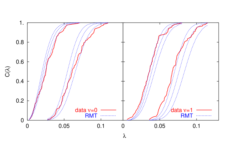
Figure 1: Cumulative distributions of the eigenvalues where $C(\lambda)$ is the fraction of all gauge configurations where the n-th eigenvalue is smaller than $|\lambda|$. We show the data for $n=1$ and $2$ for topological sector $\nu=0$ and 1. The dotted lines are the predictions from RMT with the value of $\Sigma a^{3}$ obtained from fits to the data (from left to right: fits C, B, A from Table 1).

Fit	$\Sigma$	$|\nu|$	level 1	level 2
A	0.0087(4)	0	0.87	0.02
		1	$2\cdot 10^{-5}$	0
B	0.0096(3)	0	0.04	0.004
		1	0.21	$1\cdot 10^{-5}$
C	0.0102(4)	0	$2\cdot 10^{-4}$	$2\cdot 10^{-6}$
		1	0.59	0.21

Table 1: The confidence level of the individual distributions from the various fits. The values for levels included in the fits are boxed.

Figure 2: Binned eigenvalue distributions and the RMT prediction with $\Sigma a^{3}$ from the fit to the lowest level in each topological sector (fit B from the table).

The results of our fits are presented in Table 1 and Figs. 1, 2. From a fit to the lowest level in $\nu=0$ alone (fit A) we extract $\Sigma a^{3}=0.0087(4)$ with a confidence level(CL) of 0.87. This means that the shape of the extracted curve is in very good agreement with the theoretical prediction for the given statistics. The second level in $\nu=0$ has a CL of 0.02, which is low but still acceptable. A fit to the lowest level in $|\nu|=1$ (fit C) gives $a^{3}\Sigma a^{3}=0.0102(4)$ and a CL for the lowest two level of 0.59 and 0.21. From a combined fit to the lowest level in each sector (fit B) we get $\Sigma a^{3}=0.0096(3)$. Even with the extracted values of $\Sigma a^{3}$ seemingly apart, it is still possible that they are compatible with another, because there is no correlation between the $\nu=0$ and $|\nu|=1$ ensembles.

Now that we have determined the optimal $\Sigma a^{3}$, the quality of the fits has to tell us whether the RMT description of the data is valid. A possible source for a deviation from the RMT prediction is a too small volume. Since we simulate at finite volume, we only expect the lowest few eigenvalues to match the RMT curves. We observe that for the fits to one level alone, the fit to the second eigenvalue in the same topological sector still has an acceptable confidence level. The match between the $\Sigma$ in $\nu=0$ and $|\nu|=1$ does not seem convincing. However, one has to keep in mind that the lowest two eigenvalues are calculated on the same gauge configurations and therefore are correlated. On the other hand, there is no correlation between the extraction in the two topological sectors. This can give rise to an apparent better match between the distributions of the two levels in one topological sector as compared to the match between the lowest level in both sectors. Within our statistics, RMT seems to be applicable to the lowest eigenvalue in $\nu=0$ and $|\nu|=1$ and the second lowest eigenvalue in $\nu=0$. Nevertheless, it is well possible that the volume is still too small.

A main concern in any lattice calculation—and in particular ones using new actions and algorithms—is the auto-correlation between consecutive configurations. From our Markov chains, we saved every fifth configuration. To find out whether this separation is enough, we used the following technique: We split the data set into two sub-sets, one consisting of all the even numbered configurations and one of the odd numbered. A fit to the lowest eigenvalue in $\nu=0$ and $|\nu|=1$ on the even and the odd numbered sample gives $a^{3}\Sigma=0.0099(5)$ and 0.0094(4) respectively. The central values are almost one sigma apart suggesting a weak correlation.

To make a more quantitative statement, we have computed $a^{3}\Sigma$ on matched Bootstrap samples (where if configuration $2i$ is part of the ”even” Bootstrap sample, so is $2i+1$ in the odd sample). Correlations between the two samples should show up as correlations between the $\Sigma$ on the corresponding bootstrap samples. We therefore measured the correlation matrix element (averaging over all bootstrap samples)

$$C=\langle(a^{3}\Sigma_{\rm even}-a^{3}\bar{\Sigma}_{\rm even})(a^{3}\Sigma_{\rm odd}-a^{3}\bar{\Sigma}_{\rm odd})\rangle$$ (11)

and found $C/(a^{6}\bar{\Sigma}_{\rm even}\bar{\Sigma}_{\rm odd})=0.0007(15)$ which is zero within errors. Thus, we do not find any effects of auto-correlation beyond the five trajectories by which we spaced our measurements.

In a second test of autocorrelations, we computed the integrated autocorrelation time for individual eigenvalues from the data stream. We found integrated autocorrelation times averaging about 1.5 (in units of the collection time, 5 trajectories), with an uncertainty of about 0.7. This again suggests a weak correlation between successive measurements of eigenvalues. From this analysis we conclude that the value of the condensate in lattice units is $a^{3}\Sigma=0.0096(3)$.

II.3 The length scale

As discussed above, an overall scale is obtained from the static quark potential. The latter is extracted from the effective masses of Wilson loops after one level of HYP smearing Hasenfratz:2001hp ; Hasenfratz:2001tw , where the short-distance effects of the HYP smearing are corrected using a fit to the perturbative lattice artifacts. We measured the potential on 200 $8^{3}\times 12$ configurations at $am_{q}=0.05$ with the result shown in Fig. 3. From the parameters of the fit we obtain $r_{0}/a=3.37(10)$ for the Sommer parameter (3) and $a\sqrt{\sigma}=0.318(25)$ for the string tension. With $r_{0}=0.5$ fm, this gives a lattice spacing of $a=0.15$ fm.

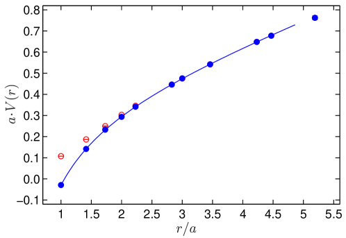
Figure 3: The static quark potential in lattice units. The filled symbols denote the potential after removing the artifacts introduced by the HYP smearing.

II.4 Matching lattice and continuum regularizations

A matching factor is needed to convert the lattice calculation of the quark condensate to its corresponding $\overline{\rm MS}$ value. To get the matching factor, we use the RI’ scheme introduced in Ref. Martinelli:1994ty , and we follow the procedure described in Ref. DeGrand:2005af , in which we calculated the matching factors for a quenched simulation. The RI’ scheme results in the chiral limit can be converted to $\overline{\rm MS}$ values at $\mu=2$ GeV by using the ratios connecting the two schemes. The ratios were computed by continuum perturbation theory to three loops Franco:1998bm ; Chetyrkin:1999pq .

These simulations should not be restricted in topological sectors. To produce a matching factor, one needs simulations with a momentum scale short enough to be free from nonperturbative effects and yet not so short as to be affected by discretization errors. Our data set consisted of 57 $8^{4}$ configurations from about 300 trajectories at $am_{q}=0.05$.

The $8^{4}$ lattice is periodic in space directions and antiperiodic in the time direction. Therefore the momentum values are

$$ap_{\mu}=\left(\frac{2\pi}{8}k_{x},\frac{2\pi}{8}k_{y},\frac{2\pi}{8}k_{z},\frac{\pi}{8}(2k_{t}+1)\right).$$ (12)

We choose the values of $k_{\mu}$ such that the momentum values lie as close as possible to the diagonal of the Brillouin zone. The maximum value of $ap=2.256$ corresponds to $k_{\mu}=(2,1,1,1)$. The quark propagators are cast from a point source and then projected to the desired momentum values.

$Z_{S}^{\rm RI^{\prime}}$ for the scalar density is shown in Fig. 4.

Figure 4: $Z_{S}^{\rm RI^{\prime}}$ for the one flavor overlap simulation.

The values of $Z_{S}^{\rm RI^{\prime}}$ are listed in Table 2. From our lattice spacing determined from the Sommer parameter, $\mu=2$ GeV corresponds to $a\mu=1.504$. The 2 GeV RI’ value is obtained from a linear interpolation from the two closest $a\mu$ points of the data. The result is $Z_{S}^{\rm RI^{\prime}}(2~{}{\rm GeV})=0.75(3)$.

Table 2: Values of $Z_{S}$ in the RI’ scheme. The inverse lattice spacing is 1.330 GeV from the Sommer parameter. Therefore $\mu=2$ GeV corresponds to $a\mu=1.504$. The value at this point is obtained from a linear interpolation from the two closest $a\mu$ points of the data.

$a\mu$	0.878	1.178	1.416	1.619
$Z_{S}^{RI^{\prime}}$	0.76(6)	0.72(4)	0.73(3)	0.78(3)
$a\mu$	1.800	1.963	2.115	2.256
$Z_{S}^{RI^{\prime}}$	0.78(2)	0.772(15)	0.777(17)	0.780(11)

The conversion ratio from the RI’ to the $\overline{\rm MS}$ scheme for the scalar and pseudoscalar densities, from Franco:1998bm ; Chetyrkin:1999pq , needs an $\alpha_{s}$. In Landau gauge and to three loops, and for one flavor, the ratio is given by

$$\frac{Z_{S}^{\overline{\rm MS}}}{Z_{S}^{\rm RI^{\prime}}} = \frac{Z_{P}^{\overline{\rm MS}}}{Z_{P}^{\rm RI^{\prime}}}=1+\frac{16}{3}\frac{\alpha_{s}}{4\pi}+\left(\frac{1375}{6}-\frac{152\zeta_{3}}{3}\right)\left(\frac{\alpha_{s}}{4\pi}\right)^{2}$$ (13)

$$+\left(\frac{32149271}{2916}-\frac{215489\zeta_{3}}{54}-\frac{80\zeta_{4}}{3}+\frac{2960\zeta_{5}}{9}\right)\left(\frac{\alpha_{s}}{4\pi}\right)^{3}+O(\alpha_{s}^{4}),$$

where $\zeta_{n}$ is the Riemann zeta function evaluated at $n$.

To get numerical results of the above ratio, we use the coupling constant from the so-called “$\alpha_{V}$” scheme. As in the appendix of Ref. DeGrand:2005vb , from the one-loop expression relating the plaquette to the coupling

$$\ln\frac{1}{3}{\rm Tr}U_{p}=-\frac{8\pi}{3}\alpha_{V}(q^{*})W,$$ (14)

where $W=0.366$ and $q^{*}a=3.32$ for the tree-level Lüscher Weisz action, we obtain $\alpha_{V}(3.32/a)=0.173$. Then $a\Lambda_{\overline{MS}}$ is calculated and $\alpha_{s}^{\overline{\rm MS}}$(2 GeV) is determined by using $\beta_{0}=31/12\pi$ and $\beta_{1}=268/48\pi^{2}$ for one flavor QCD. We find $\alpha_{s}^{\overline{\rm MS}}$(2 GeV)$=0.194$. Substituting $\alpha_{s}^{\overline{\rm MS}}$ into Eq. (13), we get $Z_{S}^{\overline{\rm MS}}/Z_{S}^{\rm RI^{\prime}}=1.147$ and therefore $Z_{S}^{\overline{\rm MS}}(2~{}{\rm GeV})=0.86(3)$.

III Results

From Sec. II the continuum-regularized condensate is

$$r_{0}^{3}\Sigma(\overline{MS},\mu=2\ {\rm GeV}) = Z_{s}(\mu,a)\times\Sigma a^{3}\times(\frac{r_{0}}{a})^{3}$$ (15)

$$= 0.86(3)\times 0.0096(3)\times(3.37(10))^{3}$$

$$= 0.317(32).$$

Taking the real-world value for $r_{0}=0.5$ fm, this is

$$\Sigma(\overline{MS},\mu=2\ {\rm GeV})=0.0194(20){\rm GeV}^{3}$$ (16)

or

$$(\Sigma(\overline{MS},\mu=2\ {\rm GeV}))^{1/3}=0.269(9){\rm GeV}.$$ (17)

IV Conclusions

Our result is in remarkable agreement with the central value of Eq. (1). Thus at least for the condensate the $1\pm 1/N_{c}$ estimates of the correction to the large $N_{c}$ result, the extreme values of Eq. (1), seem to be quite pessimistic. In view of this finding more predictions from large $N_{c}$ orientifold QCD might be interesting even without the knowledge of the subleading corrections.

A summary of previous calculations of the condensate has recently been given by McNeile McNeile:2005pd . Comparing the quenched determinations there, a three-flavor prediction by McNeile, and our result, the condensate seems to be a quantity which is not very $N_{f}$ dependent.

Other tests of orientifold equivalence will be difficult. To check the prediction of Ref. Armoni:2003fb that $m_{\eta^{\prime}}^{2}/m_{\sigma}^{2}=1+O(1/N_{c})$ is nontrivial because it requires disconnected diagrams. A similar degeneracy of hybrids described in Ref. Gorsky:2004nb will be hard because the sources for ordinary hybrids are noisy in QCD.

References

- (1) A. Armoni, M. Shifman and G. Veneziano, Phys. Rev. Lett. 91, 191601 (2003) [arXiv:hep-th/0307097].
- (2) A. Armoni, M. Shifman and G. Veneziano, Nucl. Phys. B 667, 170 (2003) [arXiv:hep-th/0302163].
- (3) A. Armoni, M. Shifman and G. Veneziano, Phys. Lett. B 579, 384 (2004) [arXiv:hep-th/0309013].
- (4) A. Armoni, M. Shifman and G. Veneziano, Phys. Rev. D 71, 045015 (2005) [arXiv:hep-th/0412203].
- (5) G. ’t Hooft, Nucl. Phys. B 75, 461 (1974).
- (6) A. Patella, arXiv:hep-lat/0511037.
- (7) H. Leutwyler and A. Smilga, Phys. Rev. D 46, 5607 (1992).
- (8) Z. Fodor, S. D. Katz and K. K. Szabo, JHEP 0408, 003 (2004) [arXiv:hep-lat/0311010].
- (9) A. Bode, U. M. Heller, R. G. Edwards and R. Narayanan, arXiv:hep-lat/9912043.
- (10) T. DeGrand and S. Schaefer, arXiv:hep-lat/0604015.
- (11) E. V. Shuryak and J. J. M. Verbaarschot, Nucl. Phys. A 560, 306 (1993) [arXiv:hep-th/9212088].
- (12) J. J. M. Verbaarschot and I. Zahed, Phys. Rev. Lett. 70, 3852 (1993) [arXiv:hep-th/9303012].
- (13) J. J. M. Verbaarschot, Phys. Rev. Lett. 72, 2531 (1994) [arXiv:hep-th/9401059].
- (14) P. H. Damgaard, U. M. Heller, R. Niclasen and K. Rummukainen, Phys. Lett. B 495, 263 (2000) [arXiv:hep-lat/0007041].
- (15) P. H. Damgaard and S. M. Nishigaki, Phys. Rev. D 63, 045012 (2001) [arXiv:hep-th/0006111].
- (16) R. Sommer, Nucl. Phys. B 411, 839 (1994) [arXiv:hep-lat/9310022].
- (17) G. Martinelli, C. Pittori, C. T. Sachrajda, M. Testa and A. Vladikas, Nucl. Phys. B 445, 81 (1995) [arXiv:hep-lat/9411010].
- (18) H. Neuberger, Phys. Lett. B 417, 141 (1998) [arXiv:hep-lat/9707022].
- (19) H. Neuberger, Phys. Rev. Lett. 81, 4060 (1998) [arXiv:hep-lat/9806025].
- (20) P. H. Ginsparg and K. G. Wilson, Phys. Rev. D 25, 2649 (1982).
- (21) S. Duane, A. D. Kennedy, B. J. Pendleton and D. Roweth, Phys. Lett. B 195, 216 (1987).
- (22) T. DeGrand and S. Schaefer, Phys. Rev. D 71, 034507 (2005) [arXiv:hep-lat/0412005].
- (23) T. DeGrand and S. Schaefer, Phys. Rev. D 72, 054503 (2005) [arXiv:hep-lat/0506021].
- (24) S. Schaefer and T. DeGrand, PoS LAT2005, 140 (2005) [arXiv:hep-lat/0508025].
- (25) M. Hasenbusch, Phys. Lett. B 519, 177 (2001) [arXiv:hep-lat/0107019].
- (26) C. Urbach, K. Jansen, A. Shindler and U. Wenger, arXiv:hep-lat/0506011.
- (27) C. Morningstar and M. J. Peardon, Phys. Rev. D 69, 054501 (2004) [arXiv:hep-lat/0311018].
- (28) M. Lüscher and P. Weisz, Commun. Math. Phys. 97, 59 (1985) [Erratum-ibid. 98, 433 (1985)].
- (29) M. G. Alford, W. Dimm, G. P. Lepage, G. Hockney and P. B. Mackenzie, Phys. Lett. B 361, 87 (1995) [arXiv:hep-lat/9507010].
- (30) C. W. Bernard and T. A. DeGrand, Nucl. Phys. Proc. Suppl. 83, 845 (2000) [arXiv:hep-lat/9909083].
- (31) W. Bietenholz, K. Jansen and S. Shcheredin, JHEP 0307, 033 (2003) [arXiv:hep-lat/0306022].
- (32) Numerical Recipes in C: The art of scientific computing, 2nd ed, W.H. Press, S.A. Teukolsky, W.T. Vetterling and B.P. Flannery, Cambridge Univ. Pr., 1995.
- (33) A. Hasenfratz and F. Knechtli, Phys. Rev. D 64, 034504 (2001) [arXiv:hep-lat/0103029].
- (34) A. Hasenfratz, R. Hoffmann and F. Knechtli, Nucl. Phys. Proc. Suppl. 106, 418 (2002) [arXiv:hep-lat/0110168].
- (35) T. DeGrand and Z. F. Liu, Phys. Rev. D 72, 054508 (2005) [arXiv:hep-lat/0507017].
- (36) E. Franco and V. Lubicz, Nucl. Phys. B 531, 641 (1998) [arXiv:hep-ph/9803491].
- (37) K. G. Chetyrkin and A. Retey, Nucl. Phys. B 583, 3 (2000) [arXiv:hep-ph/9910332].
- (38) C. McNeile, Phys. Lett. B 619, 124 (2005) [arXiv:hep-lat/0504006].
- (39) A. Gorsky and M. Shifman, Phys. Rev. D 71, 025009 (2005) [arXiv:hep-th/0410099].