QCD with Bosonic Quarks at Nonzero Chemical Potential

Abstract

We formulate the low energy limit of QCD like partition functions with bosonic quarks at nonzero chemical potential. The partition functions are evaluated in the parameter domain that is dominated by the zero momentum modes of the Goldstone fields. We find that partition functions with bosonic quarks differ structurally from partition functions with fermionic quarks. Contrary to the theory with one fermionic flavor, where the partition function in this domain does not depend on the chemical potential, a phase transition takes place in the theory with one bosonic flavor when the chemical potential is equal to $m_{\pi}/2$. For a pair of conjugate bosonic flavors the partition function shows no phase transition, whereas the fermionic counterpart has a phase transition at $\mu=m_{\pi}/2$. The difference between the bosonic theories and the fermionic ones originates from the convergence requirements of bosonic integrals resulting in a noncompact Goldstone manifold and a covariant derivative with the commutator replaced by an anti-commutator. For one bosonic flavor the partition function is evaluated using a random matrix representation.

I Introduction

Bosonic quarks appear in QCD whenever the weight of the partition function includes an inverse determinant of the Dirac operator. Ratios of determinants occur frequently in analytical approaches to QCD. Inverse determinants are for example used to quench a flavor from the theory SUSY ; replica . This form of quenching is useful in describing quenched and partially quenched PQ ; replicaPQ lattice results and is an essential ingredient when computing the spectral properties of the QCD Dirac operator. In particular, if we consider the spectral correlation functions of the Dirac operator in the microscopic limit LS ; SV , the theories with bosonic flavors are not only a part of the calculation, they are also part of the result SplitVerb1 ; SplitVerb2 ; SplitVerb3 .

The microscopic limit is an extreme version of the chiral limit where the sea and valence quark masses times the volume are kept fixed as the volume is taken to infinity. In this limit the zero modes of the Goldstone bosons associated with chiral symmetry breaking dominate the low energy partition function which reduces to a group integral uniquely determined by the pattern of chiral symmetry breaking GLeps . Sometimes this limit is referred to as the $\epsilon$-limit but since the term microscopic limit appeared earlier in the literature (see for example Efetov ; VZ ) we prefer to use this term. For a review of QCD in the microscopic limit see Tilo-Jac .

In this paper we will consider the low energy limit of QCD at nonzero chemical potential. For fermionic quark flavors the baryon chemical potential does not affect the low energy effective partition function at zero temperature. The reason is that the lightest degrees of freedom (the pions) have zero baryon charge. Because the fermion determinant is complex, QCD at nonzero baryon chemical potential cannot be simulated directly on the lattice by probabilistic methods. That is why sometimes a theory is considered where the fermion determinant is replaced by its absolute value. For an even number of flavors this corresponds to the product of a fermion determinant and its complex conjugate in the weight of the partition function. The low energy partition function for QCD with flavors and conjugate flavors depends on the chemical potential misha . The conjugate fermionic flavors correspond to ordinary fermionic flavors with the opposite sign of the chemical potential AKW . A theory with one fermionic flavor and a conjugate fermionic flavor is therefore identical to a theory with two fermionic flavors at nonzero isospin chemical potential. Since the pions have nonzero isospin charge this low energy effective partition function depends on the chemical potential. In particular, a phase transition to a Bose-Einstein condensed phase takes place at zero temperature when the isospin chemical potential reaches $m_{\pi}/2$, see misha ; KST ; KSTVZ ; eff ; lattice .

In this paper we examine the properties of the low energy QCD partition function with bosonic quarks at nonzero chemical potential. We find that the bosonic theories behave completely different from their fermionic counterparts. The bosonic partition functions depend on the chemical potential even in the absence of conjugate bosonic flavors. By explicit computation of the partition function with one bosonic flavor in the microscopic limit we find that this theory has a phase transition when the chemical potential, $\mu$, reaches $m_{\pi}/2$. On the contrary, in the theory with one conjugate pair of bosonic quarks we find that the free energy as well as its derivative are continuous at $\mu=m_{\pi}/2$ and zero temperature. The difference in the phase structure between the bosonic and the fermionic theories has its origin in the convergence requirements of bosonic integrals which forces us to rewrite the determinants in the partition function as the determinant of a Hermitian matrix (also known as hermitization Feinberg ; Janik ; Efetov-direct ). This procedure leads to a noncompact Goldstone manifold and, as will be shown here, a covariant derivative where the commutator is replaced by an anti-commutator. A comparison of bosonic and fermionic partition functions is given in table 1.

In order to compute the partition function with one bosonic flavor we make use of the random matrix representation. All other partition functions discussed here have been derived directly from the low energy effective theory.

The outline of this paper is as follows. We first discuss in general terms the low energy physics of QCD with bosonic quarks at nonzero chemical potential. As a warm up exercise we review results for fermionic quarks at nonzero chemical potential. We then turn to the theories with conjugate pairs of quarks. In section VI we present a random matrix model and perform the calculation of the partition function with one bosonic flavor in the microscopic limit. Taking the thermodynamic limit of this result then allows us to examine the phase diagram of QCD with one bosonic quark.

II General Discussion

In this section we give a general discussion of QCD-like partition functions at nonzero chemical potential. The Euclidean QCD partition function at nonzero chemical potential for $N_{f}$ flavors with mass $m$ is given by

$$Z^{N_{f}}(m;\mu)=\langle{\det}^{N_{f}}(D+\mu\gamma_{0}+m)\rangle.$$ (1)

Here and below $\langle\ldots\rangle$ denotes the average with respect to the Yang-Mills action. If $N_{f}>0$ the quarks are fermions while for negative $N_{f}$ they are interpreted as bosons. With fermionic quarks at zero temperature this partition function is independent of the chemical potential for $\mu<m_{N}/3$, which immediately follows from the definition of the grand canonical partition function as an average over Boltzmann factors and fugacities. In terms of the representation (1), the $\mu$-independence of the free energy in the thermodynamic limit can be understood from the gauge transformation

$$D+\mu\gamma_{0}+m=e^{-\mu t}[D+m]e^{\mu t},$$ (2)

so that the factor $\exp(\pm\mu t)$ can be absorbed in the boundary conditions of the fermionic fields. In the phase that is not sensitive to the boundaries, the partition function does not depend on $\mu$. A nonzero baryon density is obtained by baryons winding around the torus in the time direction. In this phase the boundary conditions are important and the partition function becomes $\mu$-dependent.

The second partition function we consider is the phase quenched partition function (the superscript $n$ counts the pairs of conjugate fermionic, $n>0$, or bosonic, $n<0$, determinants)

$$Z^{n=1}(m,m^{*};\mu)=\langle\det(D+\mu\gamma_{0}+m)\det(D+\mu\gamma_{0}+m)^{\dagger}\rangle=\langle\det(D+\mu\gamma_{0}+m)\det(-D+\mu\gamma_{0}+m^{*})\rangle,$$ (3)

so that $\mu$ can be interpreted as the isospin chemical potential AKW . Also in this case the chemical potential can be gauged into the boundary conditions, this time by a gauge transformation in isospin space. For $\mu<m_{\pi}/2$ the partition function is $\mu$-independent at zero temperature. Again, this also follows from the zero temperature limit of the Boltzmann factors.

Next, let us consider the bosonic partition function

$$Z^{n=-1}(m,m^{*};\mu)=\langle\frac{1}{\det(D+\mu\gamma_{0}+m)\det(D+\mu\gamma_{0}+m)^{\dagger}}\rangle=\langle\frac{1}{\det(D+\mu\gamma_{0}+m)\det(-D+\mu\gamma_{0}+m^{*})}\rangle.$$ (4)

Because of the nonhermiticity, the inverse determinants cannot be written directly as a convergent bosonic integral. However, this can be achieved by introducing the infinitesimal regulator $\epsilon$

$$Z^{n=-1}(m,m^{*};\mu)=\left\langle\det\left(\begin{array}[]{cc}\epsilon&D+\mu\gamma_{0}+m\\ -D+\mu\gamma_{0}+m^{*}&\epsilon\end{array}\right)^{-1}\right\rangle.$$ (7)

The parameter $\epsilon$ may be regarded as source for pions composed of bosonic anti-quarks and conjugate bosonic quarks. Expressing the partition function as an integral over the eigenvalues of the Hermitian matrix in (7) one can easily convince oneself that the partition function diverges logarithmically in $\epsilon$. In SplitVerb2 this was shown explicitly by performing the integrals in the low-energy limit of this partition function. Because of the $\epsilon$-term it is not possible to gauge away the $\mu$-dependence of the partition function, and we do not expect to find a phase where the partition function is $\mu$-independent. Indeed, we show below that the partition function (7) is $\mu$-dependent for all values of $\mu$. Therefore the pion condensate, which has $\epsilon$ as source term, is nonzero for all values of $\mu$. In particular this implies that there must be a massless mode in the spectrum. We identify this mode explicitly below.

Finally, we discuss the partition function

$$Z^{N_{f}=-1}(m;\mu)=\left\langle\frac{1}{\det(D+\mu\gamma_{0}+m)}\right\rangle.$$ (8)

It is not possible to write this partition function as a convergent bosonic quark integral. To properly define the partition function we have to rewrite it as

$$Z^{N_{f}=-1}(m;\mu)=\left\langle\frac{\det(-D+\mu\gamma_{0}+m^{*})}{\det(D+\mu\gamma_{0}+m)\det(-D+\mu\gamma_{0}+m^{*})}\right\rangle$$ (9)

so that the inverse determinant can be represented as a bosonic integral after it has been regularized as in (7). The particle content of this partition function is one conjugate fermionic quark, one bosonic quark, and one conjugate bosonic quark. Because of the extra determinant in the numerator, the limit $\epsilon\to 0$ is finite in this case, i.e. the leading term is of order $\epsilon^{0}$. In the partition function the gauge symmetry therefore allows us to transform the $\mu$ dependence to the boundaries allowing for a phase transition to occur. As we will show below a phase exists where this partition function does not depend on $\mu$. For $\mu>m_{\pi}/2$ this phase gives way to a $\mu$ dependent phase.

A summary of the different partition functions discussed in this section is given in the table below.

Theory	Number of Charged Goldstone	Critical Chemical Potential
	Modes for $\mu<\mu_{c}$
$\langle\det(D+\mu\gamma_{0}+m)\rangle$	0	$\mu_{c}=\frac{1}{3}m_{N}$
$\langle|\det(D+\mu\gamma_{0}+m)|^{2}\rangle\ \ \$	$2$	$\mu_{c}=\frac{1}{2}m_{\pi}$
$\langle\frac{1}{\det(D+\mu\gamma_{0}+m)}\rangle$	$4$	$\mu_{c}=\frac{1}{2}m_{\pi}$
$\langle\frac{1}{|\det(D+\mu\gamma_{0}+m)|^{2}}\rangle$	non applicable	$\mu_{c}=0$

Table 1: Summary of properties of low energy QCD at nonzero chemical potential and zero temperature.

Notice that the regularization enters because the chemical potential breaks the hermiticity properties of the Dirac operator. If we where to consider an imaginary chemical potential, the Dirac spectrum would remain on the imaginary axis and no regularization of the bosonic theories would be required DHSS .

III Fermionic Partition Functions

In the microscopic limit the zero momentum modes of the pions dominate the low energy effective partition function of QCD in the sense that the nonzero momentum modes factorize from the partition function leaving us with a group integral over the zero momentum modes. This integral is uniquely determined by the pattern of chiral symmetry breaking, and in the case of bosonic quarks, by the convergence of the integrals. Before turning to the theories with bosonic quarks, as a warm-up exercise, we recall results obtained for fermionic quarks. The emergence of the phase structure is discussed as well.

With fermionic quarks the partition function is automatically convergent and we need only worry about the symmetries. The Lagrangian is determined by local gauge invariance in isospin space KST . For $N_{f}+n$ ordinary fermionic quarks and $n$ conjugate fermionic quarks it is given by TV

$${\cal L}=\frac{1}{4}F_{\pi}^{2}{\rm Tr}\nabla_{\nu}U\nabla_{\nu}U^{-1}-\frac{\Sigma}{2}{\rm Tr}M(U+U^{-1})$$ (10)

with $U\in SU(N_{f}+2n)$, and the quark mass matrix is given by $M$=diag$(m_{1},\ldots,m_{N_{f}},\{z\}_{n},\{z^{*}\}_{n})$. The charge matrix $B$ is the diagonal matrix $B={\rm diag}(1,\cdots,1_{N_{f}+n},-1,\cdots,-1_{n})$. The chiral Lagrangian is parameterized by two low energy constants, the chiral condensate, $\Sigma$, and the pion decay constant $F_{\pi}$. The covariant derivatives are defined by

$$\nabla_{\nu}U=\partial_{\nu}U+\mu\delta_{\nu\,0}[U,B],\qquad\nabla_{\nu}U^{-1}=\partial_{\nu}U^{-1}+\mu\delta_{\nu\,0}[U^{-1},B].$$ (11)

In the microscopic limit the nonzero momentum modes factorize from the partition function GLeps so that the zero momentum part of the partition function in the sector of zero topological charge is given by

$$Z^{N_{f},n}(\{m_{f}\},z,z^{*};\mu)=\int_{U\in U(N_{f}+2n)}dU\ \mbox{e}^{-\frac{V}{4}F_{\pi}^{2}\mu^{2}{\rm Tr}[U,B][U^{-1},B]\ +\ \frac{1}{2}\Sigma V{\rm Tr}M(U+U^{-1})}.$$ (12)

Note that the chemical potential and the quark masses only appear through the dimensionless combinations

$$\hat{\mu}\equiv\mu F_{\pi}\sqrt{V}\ \ \ {\rm and}\ \ \ \hat{M}\equiv M\Sigma V,$$ (13)

where $V$ is the volume of space-time. In the absence of conjugate quarks the charge matrix $B$ is the unit matrix and the fermionic partition function is independent of the chemical potential. For example the partition function with one fermionic flavor is LS

$$Z^{N_{f}=1}(\hat{m})=I_{0}(\hat{m}).$$ (14)

An explicit expression for fermionic partition functions was derived in SplitVerb2 ; AFV . Here we take a closer look at the simplest nontrivial example which is given by the theory with one fermionic quark and one conjugate fermionic quark both with real mass $m$,

$$Z^{n=1}(\hat{m},\hat{m};\hat{\mu})=2\mbox{e}^{2\hat{\mu}^{2}}\int_{0}^{1}dt\ t\ \mbox{e}^{-2\hat{\mu}^{2}t^{2}}I_{0}(\hat{m}t)^{2}.$$ (15)

The chiral condensate follows by differentiation of the free energy,

$$\frac{\Sigma^{n=1}(\hat{m};\hat{\mu})}{\Sigma}=\frac{1}{2}\partial_{\hat{m}}\log Z^{n=1}(\hat{m},\hat{m};\hat{\mu}).$$ (16)

In figure 1 we have plotted the chiral condensate as a function of $m$ (in units of $m_{c}=2\mu^{2}F^{2}/\Sigma$) and as a function of $\mu$ (in units of $\mu_{c}=\sqrt{m\Sigma}/(\sqrt{2}F_{\pi})$). The full curves display a smooth dependence as was to be expected for a finite volume. In the thermodynamic limit, the would-be phase transition at $m=m_{c}$ in the left figure or at $\mu=\mu_{c}$ in the right figure becomes sharp. In terms of the dimensionless variables this limit is reached for $\hat{m}\to\infty$ or $\hat{\mu}\to\infty$ and a kink develops at the expected value of $\hat{m}/(2\hat{\mu}^{2})=1$.

In order to see how the kink is recovered we take the thermodynamic limit of (15) which is given by a leading order saddle point approximation. Using the asymptotic form of the Bessel function we obtain

$$Z^{n=1}(\hat{m},\hat{m};\hat{\mu})\sim\mbox{e}^{2\hat{\mu}^{2}}\int_{0}^{1}dt\ \frac{1}{\hat{m}}\ \mbox{e}^{-2\hat{\mu}^{2}t^{2}}e^{2t\hat{m}}.$$ (17)

A phase transition occurs when the saddle point,

$$t=\frac{\hat{m}}{2\hat{\mu}^{2}},$$ (18)

hits the integration boundary at $t=1$, that is when $\hat{m}=2\hat{\mu}^{2}$. In the phase where the saddle point is inside the boundary we obtain

$$\frac{\Sigma^{n=1}(\hat{m};\hat{\mu})}{\Sigma}\sim\frac{\hat{m}}{2\hat{\mu}^{2}}.$$ (19)

If the saddle point is outside the integration domain the chiral condensate is simply given by

$$\frac{\Sigma^{n=1}(\hat{m};\hat{\mu})}{\Sigma}=1.$$ (20)

These results are shown by the dashed curves in figure 1 and are in agreement with the results obtained from chiral perturbation theory KST ; KSTVZ ; TV ; eff .

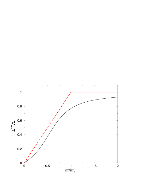
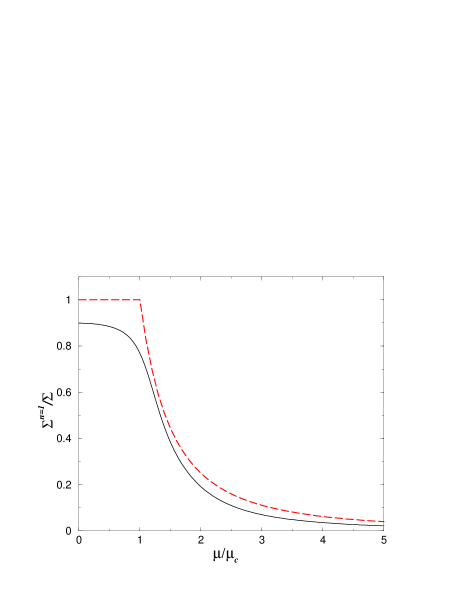
Figure 1: The chiral condensate for $n=1$ (one fermion and one conjugate fermion). Left: The mass dependence for $\hat{\mu}=\sqrt{5}$ is shown by the full curve. In the thermodynamic limit ($\hat{\mu}\to\infty$, dashed curve) the condensate grows linearly with $m$ until it reaches a plateau at $m=m_{c}=2\mu^{2}F_{\pi}^{2}/\Sigma$. Right: The full curve displays the chemical potential dependence for $\hat{m}=10$ and the dashed curve shows the result in the thermodynamic limit ($\hat{m}\to\infty$).

IV The theory with a pair of conjugate bosonic quarks

We now turn to QCD with bosonic quarks at nonzero chemical potential and start off with the theory with a pair of conjugate bosonic flavors (4). This theory is simpler than the theory with a single bosonic quark since the latter involves both fermionic and bosonic flavors (see (9)).

IV.1 Covariant Derivatives

As discussed in section II, the $n=-1$ partition function diverges. To derive the effective partition function we therefore need to take into account the convergence of the integrals in addition to the symmetries. If we write the Dirac operator as

$$D=\left(\begin{array}[]{cc}0&d\\ -d^{\dagger}&0\end{array}\right)$$ (23)

the determinant in (7) can be rearranged as

$$\left|\begin{array}[]{cccc}\epsilon&0&z&d+\mu\\ 0&\epsilon&-d^{\dagger}+\mu&z\\ z^{*}&-d+\mu&\epsilon&0\\ d^{\dagger}+\mu&z^{*}&0&\epsilon\end{array}\right|=\left|\begin{array}[]{cccc}\epsilon&z&d+\mu&0\\ z^{*}&\epsilon&0&d-\mu\\ d^{\dagger}+\mu&0&\epsilon&-z^{*}\\ 0&d^{\dagger}-\mu&-z&\epsilon\end{array}\right|.$$ (32)

For the purpose of studying the transformation properties, we rewrite the determinant of the right hand side in a $2\times 2$ block notation as

$$\left(\begin{array}[]{cc}\zeta_{1}&d+B_{1}\\ d^{\dagger}+B_{2}&\zeta_{2}\end{array}\right).$$ (35)

This operator becomes locally gauge invariant under time dependent but spatially constant flavor gauge transformations

$$\left(\begin{array}[]{cc}\zeta_{1}&d+B_{1}\\ d^{\dagger}+B_{2}&\zeta_{2}\end{array}\right)\to\left(\begin{array}[]{cc}v^{-1}&0\\ 0&u^{-1}\end{array}\right)\left(\begin{array}[]{cc}\zeta_{1}&d+B_{1}\\ d^{\dagger}+B_{2}&\zeta_{2}\end{array}\right)\left(\begin{array}[]{cc}u&0\\ 0&v\end{array}\right).$$ (44)

if $B_{1}$ and $B_{2}$ are transformed as

$$B_{1}\to vB_{1}v^{-1}-[\partial_{0}v]v^{-1}$$

$$B_{2}\to uB_{2}u^{-1}+[\partial_{0}u]u^{-1}$$ (45)

and the mass matrices are transformed as

$$\zeta_{1}\to v\zeta_{1}u^{-1}$$

$$\zeta_{2}\to u\zeta_{2}v^{-1}.$$ (46)

In SplitVerb2 we showed that the Goldstone manifold is this case is given by $Gl(2)/U(2)$. The transformation (44) induces the following transformation on the Goldstone fields

$$Q\to uQv^{-1}.$$ (47)

Therefore,

$$\partial_{0}Q\to\partial_{0}uQv^{-1}+u\partial_{0}Qv^{-1}+uQ\partial_{0}v^{-1},$$

$$\partial_{0}Q^{-1}\to\partial_{0}vQ^{-1}u^{-1}+v\partial_{0}Q^{-1}u^{-1}+vQ^{-1}\partial_{0}u^{-1}.$$ (48)

One immediately sees that the covariant combinations are

$$\partial_{0}Q-QB_{1}-B_{2}Q,$$

$$\partial_{0}Q^{-1}+B_{1}Q^{-1}+Q^{-1}B_{2}.$$ (49)

Of course $B_{1,\nu}=B_{2,\nu}=\mu\delta_{\nu\,0}\sigma_{3}\equiv\mu\delta_{\nu\,0}B$. We thus obtain the covariant derivatives

$$\nabla_{\nu}Q=\partial_{\nu}Q-\mu\delta_{\nu\,0}\{Q,B\},\qquad\nabla_{\nu}Q^{-1}=\partial_{\nu}Q^{-1}+\mu\delta_{\nu\,0}\{Q^{-1},B\}.$$ (50)

The chiral Lagrangian is the low-energy limit of QCD and should have the same covariance properties as were derived above. Taking into account terms to order $p^{2}$ in momentum counting we find the Lagrangian

$${\cal L}=-\frac{F^{2}}{4}{\rm Tr}\nabla_{\nu}Q\nabla_{\nu}Q^{-1}-\frac{i}{2}\Sigma{\rm Tr}M^{T}(Q-IQ^{-1}I)$$ (51)

with

$$M=\left(\begin{array}[]{cc}\epsilon&z\\ z^{*}&\epsilon\end{array}\right)\qquad{\rm and}\qquad I=\left(\begin{array}[]{cc}0&1\\ -1&0\end{array}\right).$$ (56)

As before, the pion decay constant is denoted by $F_{\pi}$ and the absolute value of the chiral condensate is given by $\Sigma$. We emphasize that the sign before the kinetic term is opposite to the sign of the kinetic term in the fermionic Lagrangian. This sign enters to compensate the sign due to the noncompactness of the modes in $Gl(2)/U(2)$ so that the kinetic terms pion fields have the correct sign foundations ; zirn .

In the case of the fermionic partition function with one flavor and one conjugate flavor, we also could have rearranged the fermion determinant as in (32), and we would have obtained covariant derivatives as in (50). Indeed, if we make the transformation

$$U\to U\sigma_{1}.$$ (57)

in the Lagrangian (10), the covariant derivatives in (11) change to

$$\partial_{\nu}U+\mu\delta_{\nu\,0}[U,B] \to (\partial_{\nu}U-\mu\delta_{\nu\,0}\{U,B\})\sigma_{1},$$

$$\partial_{\nu}U^{-1}+\mu\delta_{\nu\,0}[U^{-1},B] \to \sigma_{1}(\partial_{\nu}U^{-1}+\mu\delta_{\nu\,0}\{U^{-1},B\}).$$ (58)

Notice that both $U$ and $U\sigma_{1}$ are unitary. The mass term in (10) becomes

$${\rm Tr}\left(\begin{array}[]{cc}z&0\\ 0&z^{*}\end{array}\right)(U+U^{-1})={\rm Tr}M(U+\sigma_{3}U^{-1}\sigma_{3})\to{\rm Tr}\left(\begin{array}[]{cc}z&0\\ 0&z^{*}\end{array}\right)(U-\sigma_{1}\sigma_{3}U^{-1}\sigma_{3}\sigma_{1})\sigma_{1}={\rm Tr}\left(\begin{array}[]{cc}0&z^{*}\\ z&0\end{array}\right)(U+IU^{-1}I).$$ (65)

The invariance properties of this term are consistent with those of the representation (32). Because both $U$ and $-U$ belong to $U(2)$ this term has the discrete symmetry $M\to-IMI$. In the bosonic case this symmetry dictates that the relative sign of the two terms in the mass term has to be negative.

IV.2 Microscopic limit of the partition function

In the microscopic limit, the partition function is dominated by the zero momentum modes and in the sector of zero topological charge it is given by

$$Z^{n=-1}(z,z^{*};\mu)=\lim_{\epsilon\to 0}\int\frac{dQ}{{\det}^{2}Q}\theta(Q)\ \mbox{e}^{-\frac{V}{4}F_{\pi}^{2}\mu^{2}{\rm Tr}\{Q,B\}\{Q^{-1},B\}\ +\ \frac{i}{2}{V\Sigma}{\rm Tr}M^{T}(Q-IQ^{-1}I)},$$ (67)

where $dQ\theta(Q)/{\det}^{2}Q$ is the integration measure on positive definite $2\times 2$ Hermitian matrices . In the limit $\epsilon\to 0$ the integrals can be performed analytically resulting in SplitVerb2

$$Z^{n=-1}(\hat{z},\hat{z}^{*};\hat{\mu})=\log\epsilon\,\frac{e^{-2{\hat{\mu}}^{2}}}{\hat{\mu}^{2}}\exp\left(-\frac{\hat{z}^{2}+\hat{z}^{*\,2}}{8\hat{\mu}^{2}}\right)K_{0}\left(\frac{|\hat{z}|^{2}}{4\hat{\mu}^{2}}\right).$$ (68)

Using the Toda lattice equation, the product of this partition function and its fermionic counterpart gives the quenched microscopic spectral density at nonzero chemical potential. This has been confirmed beautifully by recent quenched lattice QCD simulations at nonzero chemical potential with a staggered Dirac operator tilo-james and an overlap Dirac operator tilo .

The volume dependence has dropped from the partition function (68) and no kink will develop in the thermodynamic limit. The chiral condensate is given by

$$\frac{\Sigma^{n=-1}(\hat{m};\hat{\mu})}{\Sigma} = -\frac{1}{2}\partial_{\hat{m}}\log Z^{n=-1}(\hat{m},\hat{m};\hat{\mu})$$ (69)

$$\sim \frac{\hat{m}}{2\hat{\mu}^{2}}\qquad{\rm for}\qquad\hat{m}\to\infty\ \ ,\ \ \hat{\mu}\to\infty\ \ {\rm and}\ \ \frac{\hat{m}}{2\hat{\mu}^{2}}\sim 1.$$

It follows that the low energy theory with one bosonic flavor and its conjugate does not have a phase transition as function of $\hat{\mu}$. This is to be contrasted with the fermionic counterpart which, as discussed in section III, has a phase transition at $\hat{m}=2\hat{\mu}^{2}$. Plots of the chiral condensate for $n=-1$ are shown in Fig. 2.

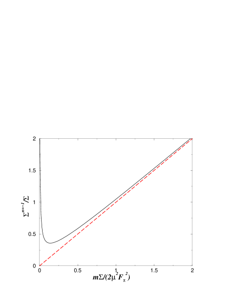
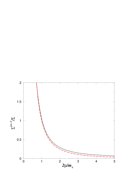
Figure 2: The chiral condensate for $n=-1$ (one boson and one conjugate boson). Left: The mass dependence for $\hat{\mu}=\sqrt{5}$ (full curve). Right: The chemical potential dependence for $\hat{m}=10$ (full curve). In this case there is no phase transition at $\mu=m_{\pi}/2$ as can be seen from the result in the thermodynamic limit (dashed curves, obtained for $\hat{\mu}\to\infty$ or $\hat{m}\to\infty$, respectively).

The reason for the absence of a phase transition at $\hat{m}=2\hat{\mu}^{2}$ becomes clear from the calculation of the mass spectrum of the Lagrangian (51) along the lines of KSTVZ (see Appendix A). For all values of the chemical potential we find a charged massless mode (in fact with a mass $\sim\sqrt{\epsilon}$) which condenses for any $\mu>0$. The masses of the remaining three modes are given by $2\mu$, $m_{\pi}^{2}/2\mu$ and $2\mu\sqrt{1+3(m_{\pi}/2\mu)^{4}}$, exactly the same as in other QCD-like theories at nonzero chemical potential KSTVZ ; eff .

V The effective partition function and chiral random matrix theory

We now turn to the computation of the partition function with one bosonic quark, that is $N_{f}=-1$. As follows from eq. (9) the Goldstone bosons result from the breaking of chiral symmetry in the theory with one fermionic and two bosonic quarks. The partition function is therefore given by an integral over the super group $\hat{Gl}(1|2)$. Such integrals are technically rather complicated, and at this point we have not succeeded to evaluate the $N_{f}=-1$ partition function along these lines.

Fortunately, the effective low energy partition function has an alternative representation as the large $N$ limit of a random matrix theory with the same chiral symmetries. This has been shown explicitly in the fermionic case at zero SV and nonzero SplitVerb2 ; O ; AFV chemical potential as well as for bosonic DV and supersymmetric OTV ; DOTV ; AF2 ; FA partition functions at zero chemical potential. For bosonic quarks at nonzero chemical potential the equivalence between the effective theories and random matrix theory in the microscopic limit has been established for $n=-1$ in AOSV .

As before, we only consider the theory in the sector of zero topological charge.

VI The Random Matrix Model

The random matrix partition function with $N_{f}$ quark flavors of mass $m$ and $n$ pairs of regular and conjugate quarks with masses $y$ and $z^{*}$, respectively, is defined by O

$${\cal Z}_{N}^{N_{f},n}(\{m_{f}\},y,z^{*};\mu) \equiv \int d\Phi d\Psi\ w_{G}(\Phi)w_{G}(\Psi){\det}^{N_{f}}(\,{\cal D}(\mu)+m_{f}\,)\$$ (70)

$$\times{\det}^{n}(\,{\cal D}(\mu)+y\,){\det}^{n}(\,{\cal D}^{\dagger}(\mu)+z^{*}),$$

where the non-Hermitian Dirac operator is given by

$$\mathcal{D}(\mu)=\left(\begin{array}[]{cc}0&i\Phi+\mu\Psi\\ i\Phi^{\dagger}+\mu\Psi^{\dagger}&0\end{array}\right)~{}.$$ (73)

Here, $\Phi$ and $\Psi$ are complex $N\times N$ matrices with the same Gaussian weight function

$$w_{G}(X)~{}=~{}\exp(\,-\,N\,{\rm Tr}\,X^{\dagger}X\,)~{}.$$ (74)

Bosonic quarks appear as inverse determinants and notationally we simply allow $N_{f}$ and $n$ to take negative values.

Of course, in general the QCD partition function and the random matrix partition function are different. However, when we consider the microscopic limit where the variables

$$\hat{m}=2mN\ \ \ {\rm and}\ \ \ \hat{\mu}^{2}=2\mu^{2}N$$ (75)

are fixed as $N\to\infty$ the random matrix partition function and the QCD partition function coincide provided that we identify (see the discussion in AOSV )

$$\hat{m}=2mN \to mV\Sigma$$ (76)

$$\hat{\mu}=2\mu^{2}N \to \mu^{2}F_{\pi}^{2}V.$$

In this section we will work within the random matrix framework and use the identifications (76) in the final results.

In O it was shown that the random matrix partition function (70) can be rewritten in the eigenvalue representation,

$${\cal Z}_{N}^{N_{f},n}(m,y,z^{*};\mu)\sim\int_{\mathbf{C}}\prod_{k=1}^{N}d^{2}z_{k}\,{\cal P}^{N_{f},n}(\{z_{i}\},\{z_{i}^{*}\};\mu),$$ (77)

where the integration extends over the full complex plane and the joint probability distribution of the eigenvalues is given by

$${\cal P}^{N_{f},n}(\{z_{i}\},\{z_{i}^{*}\};\mu) = \frac{1}{\mu^{2N}}\left|\Delta_{N}(\{z_{l}^{2}\})\right|^{2}\,\prod_{k=1}^{N}w(z_{k},z_{k}^{*};\mu)(m^{2}-z^{2}_{k})^{N_{f}}(y^{2}-z_{k}^{2})^{n}(z^{*\,2}-z_{k}^{*\,2})^{n}.$$ (78)

The Vandermonde determinant is defined as

$$\Delta_{N}(\{z^{2}_{l}\})\equiv\prod_{i>j=1}^{N}(z_{i}^{2}-z_{j}^{2}),$$ (79)

and the weight function reads

$$w(z_{k},z^{*}_{k};\mu) = |z_{k}|^{2}K_{0}\left(\frac{N(1+\mu^{2})}{2\mu^{2}}|z_{k}|^{2}\right)\exp\left(-\frac{N(1-\mu^{2})}{4\mu^{2}}(z^{2}_{k}+{{z_{k}}^{*}}^{2})\right).$$ (80)

The eigenvalue representation makes it possible to employ the method of orthogonal polynomials in the complex plane A03 ; AV ; BI ; BII ; AP to compute the spectral density and eigenvalue correlation functions O .

VI.1 Orthogonal Polynomials and their Cauchy transform

In order to evaluate the partition function with $N_{f}=-1$ we will make use of orthogonal polynomials and their Cauchy transform. The complex Laguerre polynomials given by O

$$p_{k}(z;\mu)=\left(\frac{1-\mu^{2}}{N}\right)^{k}k!L_{k}\left(-\frac{Nz^{2}}{1-\mu^{2}}\right)$$ (81)

are the orthogonal polynomials corresponding to the weight $w(z,z^{*};\mu)$ given in (80). To be specific, the polynomials satisfy the orthogonality condition Akemann

$$\int_{\mathbf{C}}d^{2}z\ w(z,z^{*};\mu)\ p_{k}(z;\mu)\ p_{l}(z;\mu)^{*}~{}\ =\ r_{k}~{}\delta_{kl}\ ,$$ (82)

with the norm

$$r_{k}~{}=~{}\frac{\pi\,\mu^{2}~{}(1+\mu^{2})^{2k}~{}k!~{}k!}{N^{2k+2}}~{}.$$ (83)

The Cauchy transform of the orthogonal polynomials is defined as

$$h_{k}(m;\mu)=\int_{\bf C}d^{2}z\frac{1}{z^{2}-m^{2}}w(z,z^{*};\mu)p^{*}_{k}(z;\mu),$$ (84)

where ${\bf C}$ indicates that the integration extends over the complex plane. Using that the weight function and polynomials are even functions of $z$ the Cauchy transform can be written as

$$h_{k}(m;\mu)=\int_{\bf C}d^{2}z\frac{1}{z(z-m)}w(z,z^{*};\mu)p^{*}_{k}(z;\mu).$$ (85)

VII QCD with one bosonic flavor

It was shown in AOSV that

$$Z_{N}^{N_{f}=-1}(m;\mu)=-\frac{1}{r_{N-1}}h_{N-1}(m;\mu).$$ (86)

Therefore, studying the properties of bosonic partition functions is equivalent to analyzing the properties of the Cauchy transform. While the relation between the partition function and the Cauchy transform was established in AOSV , no explicit evaluation of the Cauchy transform was given; this evaluation follows below. We will find that the partition function with one bosonic quark depends on the chemical potential for $\mu>m_{\pi}/2$.

We are interested in the microscopic limit where $N\to\infty$ for fixed $\hat{m}=2Nm$ and fixed $\hat{\mu}^{2}=2\mu^{2}N$. (This scaling of $\mu$ is the analogue of the weak non-hermiticity limit introduced in FKS .) In this limit the polynomial $p_{N-1}/r_{N-1}$ is given by

$$\frac{p_{N-1}(\hat{z};\hat{\mu})}{r_{N-1}} = \frac{1}{r_{N-1}}\frac{(N-1)!}{N^{N-1}}(1-\frac{\hat{\mu}^{2}}{2N})^{N-1}L_{N-1}\left(-\frac{\hat{z}^{2}}{4N}\right)$$ (87)

$$\sim \frac{2N^{5/2}e^{N}}{\sqrt{2\pi}\pi\hat{\mu}^{2}}e^{-\frac{3}{2}\hat{\mu}^{2}}I_{0}(\hat{z}),$$

where we have used that

$$r_{N-1}=\frac{\pi\hat{\mu}^{2}(1+\hat{\mu}^{2}/2N)^{2(N-1)}(N-1)!(N-1)!}{2N^{2N+1}}.$$ (88)

The microscopic limit of the partition function is thus given by

$$Z^{N_{f}=-1}(\hat{m};\hat{\mu})=-\frac{2N^{1/2}e^{N}}{\pi{\hat{\mu}}^{2}}e^{-\frac{3}{2}\hat{\mu}^{2}}\int_{\bf C}d^{2}z\frac{z^{*}}{z-\hat{m}}K_{0}\left(\frac{|z|^{2}}{4\hat{\mu}^{2}}\right)e^{-\frac{z^{2}+z^{*\,2}}{8\hat{\mu}^{2}}}I_{0}(z^{*}).$$ (89)

To calculate this integral we write (with $z=x+iy$)

$$I_{0}(z^{*})={\rm Sgn}(y)\frac{1}{\pi i}(K_{0}(z^{*})-K_{0}(-z^{*}))$$ (90)

and first calculate the integral over $y$ by a complex contour integration. The first term in (90) is exponentially damped in the upper half of the complex $y$-plane and the second term in the lower half-plane. This allows us to close the integration contour of the $y$ variable, and by Cauchy’s theorem we obtain for the real part of the partition function

$${\rm Re}(Z^{N_{f}=-1}(\hat{m};\hat{\mu}))= 2\pi c_{N}(\hat{\mu})\int_{-\infty}^{\infty}dx(2x-\hat{m})\exp[-\frac{2x^{2}-2x\hat{m}+\hat{m}^{2}}{4\hat{\mu}^{2}}]$$

$$\times \left[\theta(\hat{m}-x)\theta(2x-\hat{m})K_{0}\left(\frac{(2x-\hat{m})\hat{m}}{4\hat{\mu}^{2}}\right)I_{0}(2x-\hat{m})\right.$$ (91)

$$\left.-\theta(\hat{m}-x)\theta(\hat{m}-2x)I_{0}\left(\frac{(2x-\hat{m})\hat{m}}{4\hat{\mu}^{2}}\right)K_{0}(\hat{m}-2x)\right].$$

The imaginary part of the partition function is given by

$${\rm Im}(Z^{N_{f}=-1}(\hat{m};\hat{\mu}))= -2c_{N}(\hat{\mu})\int dx(2x-\hat{m})\exp[-\frac{2x^{2}-2x\hat{m}+\hat{m}^{2}}{4\hat{\mu}^{2}}]$$

$$\times \left[\theta(x-\hat{m})K_{0}\left(\frac{(2x-\hat{m})\hat{m}}{4\hat{\mu}^{2}}\right)K_{0}(2x-\hat{m})\right.$$ (92)

$$+\theta(\hat{m}-x)\theta(2x-\hat{m})K_{0}\left(\frac{(2x-\hat{m})\hat{m}}{4\hat{\mu}^{2}}\right)K_{0}(2x-\hat{m})$$

$$\left.+\theta(\hat{m}-x)\theta(\hat{m}-2x)K_{0}\left(\frac{(\hat{m}-2x)\hat{m}}{4\hat{\mu}^{2}}\right)K_{0}(\hat{m}-2x)\right].$$

The overall constant $c_{N}(\hat{\mu})$ is defined by

$$c_{N}(\hat{\mu})=\frac{2N^{1/2}e^{N}}{\pi{\hat{\mu}}^{2}}e^{-\frac{3}{2}\hat{\mu}^{2}}.$$ (93)

The integrand of the imaginary part is odd about $x=\hat{m}/2$ so that the integral vanishes. Using $s=x-\hat{m}/2$ as new integration variable we obtain the final expression for the partition function with $N_{f}=-1$ at nonzero chemical potential

$$Z^{N_{f}=-1}(\hat{m};\hat{\mu})= 4\pi c_{N}(\hat{\mu})e^{-\frac{\hat{m}^{2}}{8\hat{\mu}^{2}}}\int_{-\infty}^{\hat{m}/2}dss\exp[-\frac{s^{2}}{2\hat{\mu}^{2}}]$$

$$\times \left[\theta(s)K_{0}\left(\frac{s\hat{m}}{2\hat{\mu}^{2}}\right)I_{0}(2s)-\theta(-s)I_{0}\left(\frac{s\hat{m}}{2\hat{\mu}^{2}}\right)K_{0}(-2s)\right]$$

$$= 4\pi c_{N}(\hat{\mu})e^{-\frac{\hat{m}^{2}}{8\hat{\mu}^{2}}}$$

$$\times \left[\int_{0}^{\hat{m}/2}dss\exp[-\frac{s^{2}}{2\hat{\mu}^{2}}]K_{0}\left(\frac{s\hat{m}}{2\hat{\mu}^{2}}\right)I_{0}(2s)+\int_{0}^{\infty}dss\exp[-\frac{s^{2}}{2\hat{\mu}^{2}}]I_{0}\left(\frac{s\hat{m}}{2\hat{\mu}^{2}}\right)K_{0}(2s)\right].$$ (94)

VII.1 The chiral condensate for one bosonic flavor

The chiral condensate given by

$$\frac{\Sigma^{N_{f}=-1}(\hat{m};\hat{\mu})}{\Sigma}=-\partial_{\hat{m}}\log Z^{N_{f}=-1}(\hat{m};\hat{\mu})$$ (95)

is plotted in figure 3 (full curve). Notice that the chiral condensate depends on the chemical potential, and that for $\hat{m}\gg 2\hat{\mu}^{2}$, it approaches the value $\Sigma$. Below we will show that in the thermodynamic limit $\Sigma^{N_{f}=-1}$ develops a kink at $\hat{m}=2\hat{\mu}^{2}$.

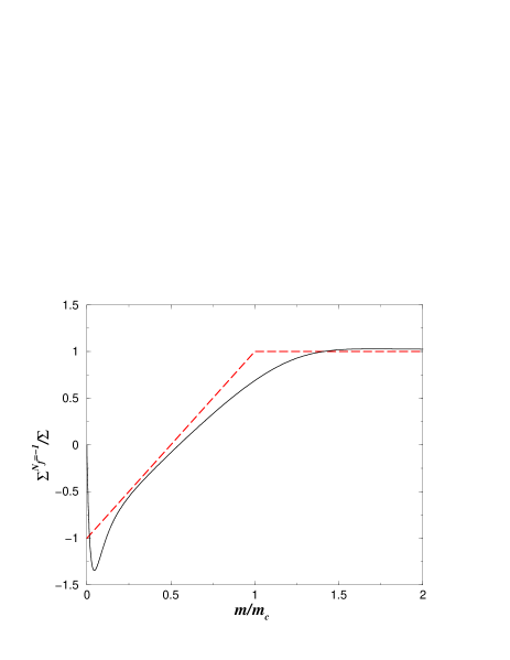
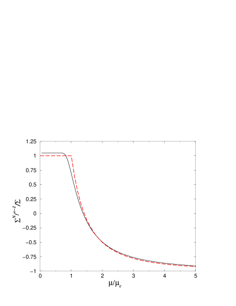
Figure 3: The chiral condensate in the theory with one bosonic flavor. Left: the mass dependence for $\hat{\mu}=\sqrt{5}$ (full curve). In the thermodynamic limit ($\hat{\mu}\to\infty$, dashed curve) $\Sigma^{N_{f}=-1}$ changes from a linear dependence on $m$ to become $m$ independent for $m>m_{c}=2\mu^{2}F_{\pi}^{2}/\Sigma$. Right: The dependence on the chemical potential for $\hat{m}=10$ (full curve) and in the thermodynamic limit ($\hat{m}\to\infty$, dashed curve).

VII.2 Phase transition with one bosonic flavor

Above we have determined the partition function in the microscopic limit, where the source $m$ times the volume $N$, is kept fixed, and as a consequence, the phase transition at $\hat{m}=2\hat{\mu}^{2}$ is smeared. A cusp in the derivative of the free energy only appears in the thermodynamic limit where $N\to\infty$ for fixed $m$. This limit can also be approached by taking $\hat{m}=2mN\to\infty$ and $\hat{\mu}^{2}=2\mu^{2}N\to\infty$ in the microscopic results as will be done below.

In the thermodynamic limit the integral (94) can be calculated by a saddle point approximation. The saddle point of the first integral is at

$$s=-\frac{\hat{m}}{2}+2\hat{\mu}^{2},$$ (96)

and the saddle point of the second integral is at

$$s=-2\hat{\mu}^{2}+\frac{\hat{m}}{2}.$$ (97)

In the thermodynamic limit the partition function for $\hat{m}>2{\hat{\mu}}^{2}$ is therefore given by

$$Z^{N_{f}=-1}(\hat{m};\hat{\mu})=\frac{4\pi}{\sqrt{2\hat{m}}}c_{N}(\hat{\mu})\mu^{2}e^{2\hat{\mu}^{2}-\hat{m}}.$$ (98)

The exponent depends linearly on $\hat{m}$ resulting in a chiral condensate that is equal to $1$. In the normalization for which the partition function is $\mu$-independent for small $\mu$ (see O ), the exponent in $c_{N}(\hat{\mu})$ (see eq. (93)) becomes $\exp(-2\hat{\mu}^{2})$ instead of $\exp(-\frac{3}{2}\hat{\mu}^{2})$. A phase transition occurs when the dominant saddle point hits the boundary of the integration domain, i.e. at $\hat{m}=2\hat{\mu}^{2}$, cf. (96). For $\hat{m}<2\hat{\mu}^{2}$ the saddle point is outside of the domain of the first integral and the main contribution to the first integral comes from the region close to $\hat{m}/2$ so that

$$Z^{N_{f}=-1}(\hat{m};\hat{\mu})\sim e^{\hat{m}-\hat{m}^{2}/2\hat{\mu}^{2}-2\hat{\mu}^{2}}\qquad{\rm for}\quad\hat{\mu}^{2}>\frac{\hat{m}}{2}.$$ (99)

The condensate in the thermodynamic limit is therefore given by

$$\frac{\Sigma^{N_{f}=-1}(\hat{m};\hat{\mu})}{\Sigma}=\left\{\begin{array}[]{ccc}-1+\frac{\hat{m}}{\hat{\mu}^{2}}&{\rm for}&\hat{m}<2\hat{\mu}^{2}\\ 1&{\rm for}&\hat{m}>2\hat{\mu}^{2}\end{array}\right..$$ (102)

In figure 3, this result is shown by the dashed curves.

As promised, we have shown that in the thermodynamic limit the chiral condensate has a kink at $\hat{m}=2\hat{\mu}^{2}$. Using (76) and the GOR-relation ($2m\Sigma=F_{\pi}^{2}m_{\pi}^{2}$) we see that the phase transition takes place at $\mu=m_{\pi}/2$ with

$$\frac{\Sigma^{N_{f}=-1}(m_{\pi};\mu)}{\Sigma}=\left\{\begin{array}[]{ccc}-1+\frac{m_{\pi}^{2}}{2\mu^{2}}&{\rm for}&m_{\pi}<2\mu\\ 1&{\rm for}&m_{\pi}>2\mu\end{array}\right..$$ (105)

This behavior of the chiral condensate can be explained from the structure in (9). We first note that the average mass derivatives of fermionic and bosonic determinants give factors that are equal in magnitude but have opposite sign. At $\mu=0$ the contribution from the fermionic quark thus cancels against the contribution from one of the bosonic quarks resulting in a total chiral condensate of magnitude $\Sigma$. For $\mu<m_{\pi}/2$ the partition function is $\mu$ independent and the chiral condensate therefore remains at the value $\Sigma$. As $\mu$ exceeds $m_{\pi}/2$ it becomes energetically favorable to create pions made out a bosonic anti-quark and a conjugate bosonic quark. As a consequence the contribution to the chiral condensate from the bosonic quarks starts rotating to zero for $\mu>m_{\pi}/2$ so that the total chiral condensate for large values of $\mu/m_{\pi}$ is given by the contribution of the fermionic flavor alone. For $\mu\gg m_{\pi}/2$ the chiral condensate therefore is equal to the chiral condensate at $\mu=0$ but with the opposite sign.

The second order phase transition can also be seen in the baryon density given by

$$\frac{n^{N_{f}=-1}(\hat{m};\hat{\mu})}{F_{\pi}}=-\partial_{\hat{\mu}}\log Z^{N_{f}=-1}(\hat{m};\hat{\mu}) = \left\{\begin{array}[]{ccc}0&{\rm for}&\hat{\mu}^{2}<\frac{\hat{m}}{2}\\ 4\hat{\mu}(1-\frac{\hat{m}^{2}}{4\hat{\mu}^{4}})&{\rm for}&\hat{\mu}^{2}>\frac{\hat{m}}{2}\end{array}\right..$$ (108)

In contrast, the free energy for $N_{f}=1$ does not depend on $\hat{\mu}$.

When $\hat{m}\sim 1$ the finite volume effects for the chiral condensate are strong and the microscopic prediction differs significantly from the result in the thermodynamic limit. For $\hat{m}\ll 1$ the partition function is given by

$$Z^{N_{f}=-1}(\hat{m};\hat{\mu})=A+\frac{\hat{m}^{2}}{8}\log\hat{m}+O(\hat{m}^{2})$$ (109)

resulting in a chiral condensate

$$\frac{\Sigma^{N_{f}=-1}(\hat{m};\hat{\mu})}{\Sigma}=\frac{1}{4A}{\hat{m}\log\hat{m}}\ \ \ {\rm for}\ \ \ \hat{m}\ll 1,$$ (110)

where $A$ is a constant. This explains the approach to zero for $\hat{m}\to 0$ of the solid curve in the left panel of Fig. 3.

VIII The phase structure and the eigenvalue spectrum

The chiral phases of QCD reflect themselves in the eigenvalue spectrum of the Dirac operator. For zero chemical potential the eigenvalue density near the origin of the imaginary axis is an order parameter for spontaneous breaking of chiral symmetry BC . When the chemical potential is nonzero the eigenvalues move into the complex plane and the chiral condensate in full QCD is then linked to the oscillations of the eigenvalue density OSV . For nonzero isospin chemical potential ($n=1$) the transition into the Bose-Einstein condensed phase takes place when the quark mass is at the boundary of the support of the eigenvalue density (see for example TV ).

Also in the case with one pair of conjugate bosons, $n=-1$, the phase structure is closely related to the Dirac spectrum. Setting $n=-1$ in (77) we obtain the following eigenvalue representation of the partition function,

$${\cal Z}_{N}^{N_{f}=0,n=-1}(z,z^{*};\mu)\sim\frac{1}{\mu^{2N}}\int_{\mathbf{C}}\prod_{k=1}^{N}d^{2}z_{k}\left|\Delta_{N}(\{z_{l}^{2}\})\right|^{2}\,\prod_{k=1}^{N}w(z_{k},z_{k}^{*};\mu)\frac{1}{(z^{2}-z_{k}^{2})(z^{*\,2}-z_{k}^{*\,2})}.$$ (111)

We observe that the probability to find an eigenvalue, $z_{j}$, has a modulus squared pole at the mass $z$. This gives rise to the logarithmic divergence discussed in section II,

$$\int_{C_{\epsilon}(u)}d^{2}u\frac{1}{|z^{2}-u^{2}|^{2}}\sim\frac{1}{|z|^{2}}\log\epsilon.$$ (112)

Here, $C_{\epsilon}(u)$ is an annulus centered at $u$ with outer radius 1 and inner radius $\epsilon\ll 1$. Because of the Vandermonde determinant, the probability that two or more eigenvalues are close to the mass $z$ does not diverge. Therefore the logarithmically divergent contribution to the partition function is from eigenvalue configurations with exactly one eigenvalue close to the mass. Setting $z_{N}=z$ in (111) and using that

$$\left.|\Delta(\{z_{l}^{2}\}_{l=1}^{N})|^{2}\right|_{z_{N}=z}=|\Delta(\{z_{l}^{2}\}_{l=1}^{N-1})|^{2}\prod_{l=1}^{N-1}|z_{l}^{2}-z^{2}|^{2},$$ (113)

we find that the product on the right hand side exactly cancels the two bosonic determinants. The remaining integral over $N-1$ eigenvalues is equal to the quenched partition function which does not depend on the mass. The only mass dependence is from the weight function, $w$, evaluated at the mass $z$ and from the divergence (112). We thus find

$${\cal Z}_{N}^{N_{f}=0,n=-1}(z,z^{*};\mu)\sim\frac{w(z,z^{*};\mu)}{|z|^{2}},$$ (114)

which is exactly the result (68) given in section IV.

The absolute value squared pole responsible for attracting the eigenvalue $z_{N}$ to the mass $z$ appears for all nonzero values of $\mu$. Hence the $n=-1$ theory must be regulated for all nonzero values of $\mu$. The transition to $\mu\to 0$ is discontinuous because if $\mu=0$ the probability to find an eigenvalue near $z$ is zero unless $z$ is on the imaginary axis.

IX Summary and Discussion

We have computed the microscopic limit (also known as the $\epsilon$-limit) of the QCD partition function at nonzero chemical potential with one bosonic quark. For the computation we made use of the random matrix representation of the partition function. Contrary to the partition function with one fermionic flavor this partition function depends on the chemical potential. In particular it has been shown that a phase transition takes place at $\mu=m_{\pi}/2$. The theory with a pair of conjugate bosonic flavors also behaves differently from its fermionic counterpart. While a phase transition signaled by Bose-Einstein condensation of pions takes place in the fermionic theory, its bosonic variant always remains in a $\mu$ dependent phase. The main differences between fermionic and bosonic partition functions have been summarized in table 1.

Bosonic partition functions as studied in this paper also appear in the closely related Hatano-Nelson model HN . This is a model for a disordered system in an imaginary vector potential. The random matrix limit of this model is a non-Hermitian random matrix model just like that in (70) except for the chiral block structure in (73). The partition function with $N_{f}=-1$ can again be expressed as the Cauchy transform of the orthogonal polynomials. However, because this model is technically simpler than the random matrix model for the QCD partition function, this partition function can also be evaluated directly by means of standard random matrix techniques. The agreement of both approaches SV-HN confirms our understanding of the Cauchy transform representation of the partition function. Moreover, as in the chiral case, we find that the partition function of the Hatano-Nelson model with $N_{f}=-1$ depends on the chemical potential and a phase transition appears in the thermodynamic limit.

These results generalize to theories with more fermionic and bosonic flavors, and we expect similar surprises for 2 color QCD and for QCD with quarks in the adjoint representation.

Our results might be relevant for a better understanding of the sign problem in QCD at nonzero baryon chemical potential. The expectation value of the phase of the fermion determinant is given by

$$\left\langle\exp(2i\theta)\right\rangle = \left\langle\frac{\det(D+\mu\gamma_{0}+m)}{\det(D+\mu\gamma_{0}+m)^{*}}\right\rangle$$ (115)

$$= \left\langle\frac{{\det}^{2}(D+\mu\gamma_{0}+m)}{\det(D+\mu\gamma_{0}+m)^{*}\det(D+\mu\gamma_{0}+m)}\right\rangle.$$

It thus corresponds to a partition function with a bosonic quark and its conjugate and two fermionic quarks. If the same arguments apply as in the case of the partition function with one bosonic flavor the vacuum expectation value of $\exp(2i\theta)$ will be nonanalytic at $\mu=m_{\pi}/2$, in the quenched as well as in the unquenched theory. We speculate that this nonanalyticity persist at nonzero temperatures and that beyond this point the severity of the sign problem increases drastically.

Note added in proof: The expectation that $\left\langle\exp(2i\theta)\right\rangle$ is nonanalytic at $\mu=m_{\pi}/2$, in the quenched as well as in the unquenched theory has now been verified phaseletter .

Acknowledgments: We wish to thank Gernot Akemann, James Osborn, Dennis Dietrich, Dominique Toublan, Poul Henrik Damgaard and Frank Wilczek for valuable discussions. Gernot Akemann is thanked for pointing out a mistake in an earlier version of this paper.This work was supported in part by U.S. DOE Grant No. DE-FG-88ER40388. KS was supported by the Carslberg Foundation.

Appendix A Calculation of the Particle Spectrum of the Chiral Lagrangian for a Pair of Bosonic Quarks

In this appendix we calculate the particle spectrum of the chiral Lagrangian (51) for QCD with a pair of conjugate bosonic quarks. We only work out in detail the case that $z=x$ is real and $\epsilon=0$.

The quark fields in the Goldstone manifold $Gl(2)/U(2)$ can be parameterized as

$$Q=\left(\begin{array}[]{cc}\cosh se^{r+t}&\sinh se^{i\theta+t}\\ \sinh se^{-i\theta+t}&\cosh se^{-r+t}\end{array}\right)\ \ \ \ \ Q^{-1}=\left(\begin{array}[]{cc}\cosh se^{-r-t}&-\sinh se^{i\theta-t}\\ -\sinh se^{-i\theta-t}&\cosh se^{r-t}\end{array}\right).$$ (120)

For the covariant derivatives we find

$$\nabla_{0}Q \equiv \partial_{0}Q-\mu\{Q,B\}$$ (123)

$$= \left(\begin{array}[]{cc}e^{r+t}[\partial_{0}\cosh s+\cosh s\partial_{0}(r+t)-2\mu\cosh s]&e^{i\theta+t}[\partial_{0}\sinh s+\sinh s\partial_{0}(i\theta+t)]\\ e^{-i\theta+t}[\partial_{0}\sinh s+\sinh s\partial_{0}(-i\theta+t)]&e^{-r+t}[\partial_{0}\cosh s+\cosh s\partial_{0}(-r+t)+2\mu\cosh s]\end{array}\right)$$

and

$$\nabla_{0}Q^{-1} \equiv \partial_{0}Q^{-1}+\mu\{Q^{-1},B\}$$ (126)

$$= \left(\begin{array}[]{cc}e^{-r-t}[\partial_{0}\cosh s-\cosh s\partial_{0}(r+t)+2\mu\cosh s]&-e^{i\theta-t}[\partial_{0}\sinh s+\sinh s\partial_{0}(i\theta-t)]\\ -e^{-i\theta-t}[\partial_{0}\sinh s-\sinh s\partial_{0}(i\theta+t)]&e^{r-t}[\partial_{0}\cosh s+\cosh s\partial_{0}(r-t)-2\mu\cosh s]\end{array}\right)$$

For the time derivatives in the kinetic term we obtain

$${\rm Tr}\nabla_{0}Q\nabla_{0}Q^{-1} = -2(\partial_{0}s)^{2}-2(\partial_{0}t)^{2}-2\cosh^{2}s(\partial_{0}r)^{2}-2\sinh^{2}s(\partial_{0}\theta)^{2}+8\mu\cosh^{2}s\partial_{0}r-8\mu^{2}\cosh^{2}s.$$ (127)

The mass term is given by

$$-i\frac{1}{2}\Sigma{\rm Tr}M^{T}(Q-IQ^{-1}I)=-i\Sigma\frac{1}{2}(4x\sinh s\cosh t\cos\theta-4y\sinh s\sinh t\sin\theta+4\epsilon\cosh r\cosh s\cosh t)$$ (128)

The total Lagrangian is

$${\bf-}\frac{F^{2}}{4}{\rm Tr}\nabla_{\mu}Q\nabla Q^{\dagger}_{\mu}-i\frac{1}{2}\Sigma{\rm Tr}M^{T}(Q-IQ^{-1}I)$$ (129)

with $M$ and $I$ defined in (56). Notice that because of the noncompact degrees of freedom, the sign of the kinetic term is opposite to the usual sign.

The static part of the Lagrangian for $y=0$ and $\epsilon=0$ is given by

$${\cal L}_{\rm static}=2F^{2}\mu^{2}\cosh^{2}s-i2\Sigma x\sinh s\cosh t\cos\theta-4\epsilon\cosh r\cosh s\cosh t.$$ (130)

The minimum is at (note that we can always divide out $\cosh s$, so there is only one minimum)

$$\sinh s=i\frac{x\Sigma}{2F^{2}\mu^{2}}=i\frac{m_{\pi}^{2}}{4\mu^{2}}$$ (131)

and

$$t=0,\quad r=0,\quad\theta=0.$$ (132)

We expand the chiral Lagrangian (129) to second order in the small fluctuations about the saddle point. The second order terms are given by

$$F^{2}[-\frac{1}{2}(\partial_{0}\delta s)^{2}-\frac{1}{2}(\partial_{0}\delta t)^{2}-\frac{1}{2}\cosh^{2}s(\partial_{0}\delta r)^{2}-\frac{1}{2}\sinh^{2}s(\partial_{0}\delta\theta)^{2}+4\mu\sinh s\cosh s\delta s\partial_{0}\delta r-2\mu^{2}(\cosh^{2}s+\sinh^{2}s)(\delta s)^{2}]$$

$$+i\Sigma x\sinh s[(\delta s)^{2}+(\delta t)^{2}-(\delta\theta)^{2}].$$ (133)

We obtain the uncoupled masses

$$m_{t}^{2} = -i\frac{2x\Sigma}{F^{2}}\sinh s=\frac{m_{\pi}^{4}}{4\mu^{2}},$$ (134)

$$m_{\theta}^{2} = 4\mu^{2}.$$ (135)

The remaining two masses of follow from solving

$$\det\left(\begin{array}[]{cc}E^{2}-4\mu^{2}\cosh^{2}s&+4\mu E\sinh s\cosh s\\ -4\mu E\sinh s\cosh s&E^{2}\cosh^{2}s\end{array}\right)=0$$ (137)

since $\cosh s\neq 0$ we can divide by $\cosh^{2}s$ and obtain

$$E^{2}(E^{2}-4\mu^{2}\cosh^{2}s)+16\mu^{2}E^{2}\sinh^{2}s=0$$ (138)

with solutions

$$E^{2}=0\quad{\rm or}\quad E^{2}=4\mu^{2}\cosh^{2}s-16\mu^{2}\sinh^{2}s=4\mu^{2}(1+\frac{3m_{\pi}^{2}}{16\mu^{4}})$$ (139)

Note that one mode is massless for all $\mu>0$. For $\epsilon\neq 0$ one can show along the same lines that the massless mode obtains a mass $\sim\sqrt{\epsilon}$.

References

- (1) K.B. Efetov, Phys. Rev. Lett. 79, 491 (1997); Adv. Phys. 32, 53 (1983), Supersymmetry in disorder and chaos, (Cambridge University Press, Cambridge, 1997).
- (2) S.F. Edwards and P.W. Anderson, J. Phys. F5, 965 (1975); S.F. Edwards and R.C. Jones, J. Phys. A 9, 1595 (1976); J.J.M. Verbaarschot and M.R. Zirnbauer, Ann. Phys. 158, 78 (1984); J.J.M. Verbaarschot and M.R. Zirnbauer, J. Phys. A 18, 1093 (1985); A. Kamenev and M. Mézard, J. Phys. A, 32, 4373 (1999); Phys. Rev. B 60, 3944 (1999); I.V. Yurkevich and I.V. Lerner, Phys. Rev. B 60, 3955 (1999); M.R. Zirnbauer [cond-mat/9903338].
- (3) C. W. Bernard and M. F. L. Golterman, Phys. Rev. D 46, 853 (1992); Phys. Rev. D 49, 486 (1994).
- (4) P.H. Damgaard and K. Splittorff, Nucl. Phys. B 572, 478 (2000); Phys. Rev. D 62, 054509 (2000); P.H. Damgaard, Phys. Lett. B 476, 465 (2000).
- (5) H. Leutwyler and A. Smilga, Phys. Rev. D 46, 5607 (1992).
- (6) E.V. Shuryak and J.J.M. Verbaarschot, Nucl. Phys. A 560, 306 (1993); J.J.M. Verbaarschot, Phys. Rev. Lett. 72, 2531 (1994).
- (7) K. Splittorff and J.J.M. Verbaarschot, Phys. Rev. Lett. 90, 041601 (2003).
- (8) K. Splittorff and J. J. M. Verbaarschot, Nucl. Phys. B 683, 467 (2004).
- (9) K. Splittorff and J. J. M. Verbaarschot, Nucl. Phys. B 695, 84 (2004).
- (10) J. Gasser and H. Leutwyler, Phys. Lett. B 188, 477 (1987).
- (11) K.B. Efetov, Adv. Phys. 32, 53 (1983).
- (12) J.J.M. Verbaarschot and M.R. Zirnbauer, Ann. Phys. 158, 78 (1984).
- (13) J. J. M. Verbaarschot and T. Wettig, Ann. Rev. Nucl. Part. Sci. 50, 343 (2000).
- (14) M. Stephanov, Phys. Rev. Lett. 76, 4472 (1996).
- (15) M. Alford, A. Kapustin, and F. Wilczek, Phys. Rev. D 59 (1999) 054502.
- (16) J.B. Kogut, M.A. Stephanov, and D. Toublan, Phys. Lett. B 464, 183 (1999).
- (17) J.B. Kogut, M.A. Stephanov, D. Toublan, J.J.M. Verbaarschot, and A. Zhitnitsky, Nucl. Phys. B 582, 477 (2000).
- (18) D. Toublan and J. J. M. Verbaarschot, Int. J. Mod. Phys. B 15, 1404 (2001).
- (19) D. T. Son and M. A. Stephanov, Phys. Rev. Lett. 86, 592 (2001); K. Splittorff, D. T. Son, and M. A. Stephanov, Phys. Rev. D 64, 016003 (2001); J. B. Kogut and D. Toublan, Phys. Rev. D 64, 034007 (2001); K. Splittorff, D. Toublan, and J.J.M. Verbaarschot, Nucl. Phys. B 620, 290 (2002); Nucl. Phys. B 639, 524 (2002); J. Wirstam, J. T. Lenaghan, K. Splittorff, Phys. Rev. D 67, 034021 (2003); J.T. Lenaghan, F. Sannino, K. Splittorff, Phys. Rev. D 65, 054002 (2002).
- (20) J.B. Kogut and D.K. Sinclair, Phys. Rev. D 66, 034505 (2002).
- (21) J. Feinberg and A. Zee, Nucl. Phys. B504, 579 (1997).
- (22) R. A. Janik, M. A. Nowak, G. Papp, J. Wambach and I. Zahed, Phys. Rev. E 55, 4100 (1997); R. A. Janik, M. A. Nowak, G. Papp and I. Zahed, Nucl. Phys. B 501, 603 (1997).
- (23) K.B. Efetov, Phys. Rev. Lett. 79, 491 (1997); Phys. Rev. B56, 9630 (1997).
- (24) P. H. Damgaard, U. M. Heller, K. Splittorff and B. Svetitsky, Phys. Rev. D 72, 091501 (2005); P. H. Damgaard, U. M. Heller, K. Splittorff, B. Svetitsky and D. Toublan, Phys. Rev. D 73, 074023 (2006); Phys. Rev. D 73, 105016 (2006).
- (25) H. Leutwyler, Annals Phys. 235, 165 (1994).
- (26) M.R. Zirnbauer, J. Math. Phys. 37, 4986 (1996).
- (27) G. Akemann, T. Wettig, Phys. Rev. Lett. 92 (2004) 102002; Erratum-ibid. 96 (2006) 029902; J. C. Osborn and T. Wettig, PoS LAT2005, 200 (2005) [arXiv:hep-lat/0510115].
- (28) J. Bloch and T. Wettig, arXiv:hep-lat/0604020.
- (29) G. Akemann, Y. V. Fyodorov and G. Vernizzi, Nucl. Phys. B 694, 59 (2004).
- (30) J. C. Osborn, Phys. Rev. Lett. 93, 222001 (2004).
- (31) D. Dalmazi and J.J.M. Verbaarschot, Nucl. Phys. B 592, 419 (2001).
- (32) J.C. Osborn, D. Toublan and J.J.M. Verbaarschot, Nucl. Phys. B 540, 317 (1999).
- (33) P.H. Damgaard, J.C. Osborn D. Toublan, and J.J.M. Verbaarschot, Nucl. Phys. B 547, 305 (1999).
- (34) G. Akemann, Y.V. Fyodorov, Nucl. Phys. B 664 (2003) 457.
- (35) Y. V. Fyodorov and G. Akemann, JETP Lett. 77, 438 (2003) [Pisma Zh. Eksp. Teor. Fiz. 77, 513 (2003)].
- (36) G. Akemann, J. C. Osborn, K. Splittorff and J. J. M. Verbaarschot, Nucl. Phys. B 712, 287 (2005).
- (37) G. Akemann and G. Vernizzi, Nucl. Phys. B 660 (2003) 532.
- (38) G. Akemann, Acta Phys. Polon. B 34 (2003) 4653.
- (39) M.C. Bergère, [hep-th/0311227].
- (40) M.C. Bergère, [hep-th/0404126].
- (41) G. Akemann and A. Pottier, J. Phys. A 37, L453 (2004).
- (42) G. Akemann, Nucl. Phys. B730 (2005) 253.
- (43) Y.V. Fyodorov, B.A. Khoruzhenko and H.-J. Sommers, Phys. Lett. A226 (1997) 46; Phys. Rev. Lett. 79 (1997) 557.
- (44) T. Banks and A. Casher, Nucl. Phys. B169, 103 (1980).
- (45) J. C. Osborn, K. Splittorff and J. J. M. Verbaarschot, Phys. Rev. Lett. 94, 202001 (2005).
- (46) J. Miller and J. Wang, Phys. Rev. Lett. 76, 1461 (1996); N. Hatano and D. R. Nelson, Phys. Rev. Lett. 77, 570 (1996).
- (47) K. Splittorff and J.J.M. Verbaarschot, in progress.
- (48) K. Splittorff and J. J. M. Verbaarschot, hep-lat/0609076.