NGN, QCD₂ and Chiral Phase Transition
from String Theory

Abstract

We construct a D2-D8-$\bar{D8}$ configuration in string theory, it can be described at low energy by two dimensional field theory. In the weak coupling region, the low energy theory is a nonlocal generalization of Gross-Neveu(GN) model which dynamically breaks the chiral flavor symmetry $U(N_{f})_{L}\times U(N_{f})_{R}$ at large $N_{c}$ and finite $N_{f}$. However, in the strong coupling region, we can use the SUGRA/Born-Infeld approximation to describe the low energy dynamics of the system. Also, we analyze the low energy dynamics about the configuration of wrapping the one direction of D2 brane on a circle with anti-periodic boundary condition of fermions. The fermions and scalars on D2 branes get mass and decouple from the low energy theory. The IR dynamics is described by the $QCD_{2}$ at weak coupling. In the opposite region, the dynamics has a holographic dual description. And we have discussed the phase transition of chiral symmetry breaking at finite temperature. Finally, after performing T-duality, this configuration is related to some other brane configurations.

May  2006

1 Introduction

The ads/cft correspondence is one of the realizations of the holographic principle. It relates string theory on some background to $N=4$ SYM theory on the boundary [1, 2], and for a review see [3]. Inspired by this correspondence, one naturally asks how to construct a holographic dual model of the given four-dimensional field theory and to study some interesting low energy physics such as confinement and spontaneous chiral symmetry breaking. Following the adf/cft, some new methods [4, 5, 6, 7] for studying strongly coupled gauge theories have been developed. In [4], Witten proposed a construction of the holographic dual of four-dimensional pure $SU(N_{c})$ YM theory. In his construction, the $N_{c}$ D4-branes wrap on a circle with antiperiodic boundary conditions for the fermions living on the D4-branes. The antiperiodic boundary conditions give a mass to fermions and scalars on the D4-branes at tree level and one loop, respectively. Below this mass scale the dynamics on the D4-branes can be described by the pure $U(N_{c})$ YM theory. But in such construction, there are no flavor degrees of freedom. Observing this, Karch and Katz introduced flavor branes to give a construction of holographic models with flavors [8]. The SUGRA/Born-Infeld approximation can be used to describe aspects of large $N_{c}$ gauge theories with finite $N_{f}$ flavors from the holographic point of view. There are many developments along this line [9, 10, 11, 12, 13, 14]. For example, in [11], M.Kruczenski, D.Mateos, R.C.Myers and D.J.Winters(KMMW) considered the D4-D6-brane configuration, and in [12], T.Sakai and S. Sugimoto(SS) proposed the D4-D8-$\bar{D8}$-branes model and wished to obtain a better understanding of $QCD_{4}$ with flavors from holographic point of view. In the SS model, the global $U(N_{f})_{L}\times U(N_{f})_{R}$ chiral flavor symmetry in $QCD_{4}$ is induced by the gauge symmetry of the $N_{f}$ D8-$\bar{D8}$-brane pairs. SS applied SUGRA approximation to analyze chiral symmetry breaking and compute the meson spectrum at zero temperature. In recently papers [15, 16, 17, 18, 19], the authors studied the phase transition in a finite temperature using the dual description. They found that at sufficiently low temperature the chiral symmetry is broken, while for temperature large than the critical value, the symmetry is restored. And this is a first order phase transition between broken and unbroken chiral symmetry phase. Also in [20], the chiral phase transition is studied in strongly-coupled large $N_{c}$ N = 4 SYM theory on a 3-sphere coupled to a finite number $N_{f}$ of massive $N=2$ hypermultiplets in the fundamental representation of the gauge group.

Recently, in [21], Antonyan et al. studied the D4-D8-$\bar{D8}$ brane configuration where the D4-branes is not compactified on a circle. In the weak ’t Hooft coupling region, the low energy dynamics of this D-brane configuration in string theory is described by the nonlocal version of Nambu-Jona-Lasinio(NJL) model [22]. The NJL model is exactly solvable at large $N_{c}$ and dynamically breaks the chiral flavor symmetry at weak ’t Hooft coupling and is non-renormalizable due to the four Fermi interaction. In the strong coupling parameter region, the SUGRA approximation is reliable. By varying the parameters, the D-brane configuration can interpolate between NJL and $QCD_{4}$.

Along this line, we are mainly interested in the two dimensional physics for example the chiral symmetry breaking in this paper. We know that the two-dimensional version of the NJL model is the Gross-Neveu(GN) model [23], which is superrenormalizable and asymptotical free without gauge fields. Since it is a vector model [24], it can be exactly solvable at large $N_{c}$ and finite $N_{f}$. Also this model breaks the chiral symmetry dynamically and generates a mass for quark via dimensional transmutation [25]. In this paper we study a D2-D8-$\bar{D8}$-brane configuration in IIA string theory. In this brane configuration, the two dimensional theory has $U(N_{f})_{L}\times U(N_{f})_{R}$ chiral symmetry which is induced from the gauge symmetry. At weak coupling, the low energy dynamics of $q_{L},q_{R}$ is described by the non-local GN(NGN) model. We can find that the fermions get mass and the chiral symmetry $U(N_{f})_{L}\times U(N_{f})_{R}$ dynamically breaks to the diagonal subgroup $U(N_{f})$. In strong coupling region, however, we can use the SUGRA to describe the dynamics and can get the similar results. Though the GN is a two-dimensional toy model, it shares many same interesting properties with the $QCD_{4}$. Hence its string realization can give us better understanding of the four-dimensional physics, especially some nonperturbative aspects, and also give us some hints about how to embed the 4D physics into sting theory and obtain some holograhic description. We will also consider another case that’s to compactify one direction of D2-branes with antiperiodic boundary conditions for fermions on the D2-branes. In this case, it will introduce another scale the radius of a circle except for the distance between the parallel D8-$\bar{D8}$-brane pairs in the low-energy theory. Thus, we need to analyze the parameters space again. At weak coupling, the low energy dynamics can be described by the two-dimensional $QCD_{2}$. However, in the opposite region, the low energy dynamics has a holographic description of $QCD_{2}$ by the supergravity. Also, we study the chiral phase transition at high temperature. There is a critical temperature, under it, the chiral symmetry is broken. But beyond this temperature, the chiral symmetry is restored. For this brane configuration, if performing T-duality along the compactified direction, we can get the D1-D9-$\bar{D9}$-brane configuration [26]. The low energy dynamics on D1-brane with $N_{c}=1$ is a two-dimensional QED theory(Schwinger model [27]). The two-dimensional QED is a exactly solvable and can apply some power techniques for example bosonization to study the D-brane dynamics. If doing a T-duality along the D1-brane worldvolume again, we get the D0-D8-$\bar{D8}$-branes configuration and have a matrix description of the dynamics of the D0-branes. There are other D-branes configurations such as D2-D6-$\bar{D6}$ and D2-D4-$\bar{D4}$-branes system [38]. The intersectional part is also two dimensions as the D2-D8-$\bar{D8}$ brane configuration. In this paper, we mainly focus on the D2-D8-$\bar{D8}$ brane configuration. But for the other brane configuration such as D2-D6-$\bar{D6}$ and D2-D4-$\bar{D4}$, one can do the same analysis as the D2-D8-$\bar{D8}$ brane configuration in the following sections of this paper.

The organization of this paper is as follows. In section 2, we explain the brane configuration and the open string spectrum of the D2-D8-$\bar{D8}$-branes system and discuss the valid region of the weak and strong-coupling approximation. And we study the low-energy dynamics at weak coupling and can find it is described by a non-local GN model which exhibits chiral symmetry breaking at weak coupling at large $N_{c}$. At strong coupling we use SUGRA/Born-Infeld approximation to study the low-energy dynamics, the fermions get mass and chiral symmetry is broken. In section 3, we give a generalization to the above configuration and compactify the one of D2-brane coordinates on a circle with antiperiodic boundary condition for the fermions on D2-branes, then the fermions and scalars on D2-branes get mass and is decoupled from the low energy theory. Also, we analyze the properties of this model at weak coupling and strong coupling region and the chiral phase transition in finite temperature. After performing T-duality, this configuration can relate to some other brane system such as the D1-D9-$\bar{D9}$, D0-D8-$\bar{D8}$-branes system. Finally, we give some comments and discussions about the results of this paper in section 4.

2 D2-D8-$\bar{D8}$ brane configuration

Now let us introduce a brane configuration in IIA string theory that are $N_{c}$ D2, $N_{f}$ D8 and $N_{f}$ $\bar{D8}$-branes. The extending directions of these branes are indicated in the following

$$\begin{array}[]{ccccccccccccc}&0&1&2&3&4&5&6&7&8&9\\ D2:&{\rm x}&{\rm x}&{\rm x}&{}\hfil&{}\hfil&{}\hfil&{}\hfil&{}\hfil&{}\hfil&{}\hfil\\ {D8,\bar{D8}}:&{\rm x}&{\rm x}&{}\hfil&{\rm x}&{\rm x}&{\rm x}&{\rm x}&{\rm x}&{\rm x}&{\rm x}\end{array}$$ (2.1)

In this brane configuration, the $N_{f}$ D8 and $\bar{D8}$-branes are parallel and separated by a distance $L$ in the $x^{2}$ direction. The $N_{c}$ D2-branes intersect with the $N_{f}$ D8-$\bar{D8}$-branes along directions $(x^{0},x^{1})$. All the others $(x^{3},x^{4},...,x^{9})$ are the transverse directions to the intersection part of this brane configuration. Here the description of the brane configuration is classically , as we will see in the following sections the quantum fluctuation can change this classical picture. In this D-branes system, the particle spectrum can be created by the open 2-2, 8-8, $\bar{8}$-$\bar{8}$, 8-$\bar{8}$, 2-8 and 2-$\bar{8}$ strings which ends on the respective D-branes. The massless spectrum generated by the p-p open strings(where p denotes 2, 8, $\bar{8}$) have worldvolume gauge fields $A_{\mu}$($\mu$= 0,…,p), scalar fields $\phi^{i}$ (i=p+1,…,9) which describe the transverse fluctuation of D-branes. Due to supersymmetry on D-brane, there exists corresponding fermions on the D-brane worldvolume. The fields of the gauge theories on the worldvolume can be obtained by dimensional reduction of $N=1U(n)$ ten dimensional SYM. All these fields transform under the adjoint representation of the gauge group $U(n)$. In this D-brane configuration, the $n$ is equal to $N_{c}$ for the 2-2 open string. But for the 8-8 and $\bar{8}$-$\bar{8}$ case, $n$ is chosen to $N_{f}$. To the 8-$\bar{8}$ open string, it may create tachyon mode. The mass of this ground state is given by $m^{2}=(\Delta x^{2}/2\pi\alpha^{\prime})^{2}-1/2\alpha^{\prime}$, where $\Delta x^{2}$ is the distance between the D8-branes and $\bar{D8}$-branes. If the distance $\Delta x^{2}>\sqrt{2}\pi l_{s}$, then one may think that this mode is massive and decouple from the low energy physics. We will give some discussions about the fundamental string in the background (2.23) in the subsection 2.2.

As for the 2-8 and 2-$\bar{8}$ open strings, in the NS-sector the massless spectrum depends on the $\#ND$ numbers of corresponding D-branes of open string ending on. From (2.1) we can get $\#ND=8$, the vacuum zero energy is $1/2$. Thus, we can see that all the states in NS-sector are massive, in the low energy theory, the NS-sector is decoupled. For the R sector, since the vacuum zero energy always vanishes, the ground state is massless. Then, the ground states in the R-sector consist of positive and negative chirality spinor representations of the Lorentz group $SO(1,1)$. Due to the GSO projection, one of these two spinors is projected out. We can choose the positive chirality spinors as physical states created by the 2-8 strings and denote the fields as $q_{L}$ localized at $x^{2}=-L/2$, which transform in the fundamental representation ($N_{c}$, $N_{f}$, 1) of the symmetry group $U(N_{c})\times U(N_{f})_{L}\times U(N_{f})_{R}$. The left-hand weyl fermion $q_{L}$ is complex since the 2-8 open strings have two orientations. Similarly, the massless right-hand weyl fermions $q_{R}$ can be created by the 2-$\bar{8}$ open strings and locate at $x^{2}=L/2$, which transform in the fundamental representation ($N_{c}$, 1, $N_{f}$) of the symmetry $U(N_{c})\times U(N_{f})_{L}\times U(N_{f})_{R}$.

We need to mention that the component $A_{2}$ of the gauge field $A_{M}(M=0,1,2)$ and the scalar fields $\phi^{i}$ on the D2-branes worldvolume can couple the quarks $q_{L}$ and $q_{R}$. But because of the shift symmetry $\phi^{i}\rightarrow\phi^{i}+const$ and gauge invariance, they can only couple to the other massless modes through irrelevant operators. In the low energy theory, the irrelevant coupling don’t play an important role. The fermions on D2-branes also don’t couple with quarks. Thus, the low energy dynamics on the two-dimensional intersection is decoupled with the IR dynamics of the scalars $\phi^{i}$, $A_{2}$ and 2-2 strings fermions on the D2-branes worldvolume.

In the following, we are interested in the physics of intersectional part of D-branes. Hence, we give a summary of all the massless modes and their transformation under gauge symmetry in the $1+1$ intersectional dimensions. They can be listed in the following table 1.

field	SO(1,1)	SO(8)	$U(N_{c})\times U(N_{f})_{L}\times U(N_{f})_{R}$
$A_{\mu}$	2	1	(adj, 1, 1 )
$q_{L}$	$1_{+}$	1	$(N_{c},N_{f},1)$
$q_{R}$	$1_{-}$	1	$(N_{c},1,N_{f})$

Table 1: the massless degrees of freedom on the intersection of this branes configuration

In the following studying, we are interested in this system at the energy much below the string scale and in the limit $g_{s}\rightarrow 0$, $N_{c}\rightarrow\infty$ with $g_{s}N_{c}$ and $N_{f}$ held fixed. In this brane configuration, the $D_{2}$-branes worldvolume theory is a three dimensional $U(N_{c})$ gauge theory with the gauge coupling constant $g_{3}^{2}=g_{s}/l_{s}$ [28]. The ’t Hooft coupling constant can be defined as $\lambda=g_{3}^{2}N_{c}/4\pi=g_{s}N_{c}/4\pi l_{s}$. Since the coupling $g_{3}^{2}$ has units of mass, then the thing is same for ’t Hooft coupling constant. Now we can analyze the coupling constant parameter space. As in [29], we can introduce energy scale $U\equiv r/\alpha^{\prime}$, at this energy scale, the effective dimensionless coupling constant in three dimensional gauge theory is $g^{2}_{eff}\approx\lambda/U$. In this brane configuration, the energy scale is the distance $L$ between D8 and $\bar{D8}$ brane. Thus, in the region

$$l_{s}\ll L\ll\frac{1}{\lambda}$$ (2.2)

the physics that we are interested lies at a distance scale much larger than the string scale $l_{s}$, we can neglect the string effects. The effective coupling constant $g^{2}_{eff}\approx\lambda L\ll 1$, the coupling is weak and the perturbative calculation can be trusted in this region. We can use the perturbative theory to describe the dynamics of quarks $q_{L}$ and $q_{R}$. If $L\rightarrow\infty$, the $g^{2}_{eff}\rightarrow\infty$, which means the interaction between the left-hand quarks and the right-hand quarks becomes strong with increasing the distance $L$. However, if let $L\rightarrow 0$, the effective coupling constant $g^{2}_{eff}\rightarrow 0$. When the ’t Hooft coupling increases into the region

$$l_{s}\ll\frac{1}{\lambda}\ll L$$

$$\frac{1}{\lambda}\ll l_{s}\ll L$$ (2.3)

the effective coupling constant becomes large and the interaction between $q_{L}$ and $q_{R}$ becomes strong. We can’t use the above perturbative way to deal with it, instead in this region we can use the SUGRA/Born-Infeld approximation to study the low energy dynamics of the brane system. In the subsection 2.2, the IR physics of the brane system in the strong coupling region can be investigated by analyzing the dynamics of D8-branes in the near-horizon geometry of the D2-branes.

2.1 Weak coupling region

In this subsection, we discuss the D2-D8-$\bar{D8}$-brane configuration in the weakly coupled region (2.2). If the distance $L$ between D8 and $\bar{D8}$-branes is approximate to zero, there are no attractive force interaction between D8 and $\bar{D8}$-branes. In this case, we only need to consider a single intersectional branch between $N_{c}$ D2-branes and $N_{f}$ D8-branes. Then the effective action of the quark $q_{L}$ and U($N_{c}$) gauge field $A_{M}$ is given by

$$S=\int{d^{3}x\left[-\frac{1}{4g^{2}_{3}}F^{2}_{MN}+i\delta(x^{2})q^{\dagger}_{L}(-D_{0}+D_{1})q_{L}\right]}$$ (2.4)

where the indices $M=0,1,2$, the covariant derivative $D_{0}$ and $D_{1}$ means $D_{\mu}=\partial_{\mu}-iA_{\mu}$ choosing $\mu=0,1$, respectively. And the branes intersection is located at $x^{2}=0$. After integrating the gauge field $A_{M}$ and approximating to first order about the gauge coupling $g^{2}_{3}$ in the gauge field Lagrangian and in the Feynman gauge, the effective action of $q_{L}$ is

$$S_{eff}=i\int d^{2}xq^{\dagger}_{L}(-\partial_{0}+\partial_{1})q_{L}$$ (2.5)

Thus, we can see , if up to first order correction, the effective action of left-hand quark is free. But if concluding the high order correction, the quarks $q_{L}$ will interact each other.

In the following we will discuss the two branches intersection case of the D2-D8-$\bar{D8}$-branes. The distance between D8 and $\bar{D8}$-branes is $L$, and they locate at $x^{2}=-L/2$ and $x^{2}=L/2$ respectively. Then the low energy effective action on the intersection of branes

$$\begin{array}[]{lll}S=&\int d^{3}x\left(-\frac{1}{4g^{2}_{3}}F^{2}_{MN}\right)\\ &+\int d^{2}x\left(i\delta(x^{2}+L/2)q^{\dagger}_{L}(-D_{0}+D_{1})q_{L}+i\delta(x^{2}-L/2)q^{\dagger}_{R}(-D_{0}-D_{1})q_{R}\right)\end{array}$$ (2.6)

Integrating out the gauge field in the single gluon exchange approximation we get

$$\begin{array}[]{lll}S_{eff}=&i\int d^{2}x\left[q^{\dagger}_{L}(-\partial_{0}+\partial_{1})q_{L}+q^{\dagger}_{R}(-\partial_{0}-\partial_{1})q_{R}\right]\\ &~{}~{}~{}~{}~{}~{}~{}~{}~{}+\frac{g^{2}_{3}}{4\pi}\int d^{2}xd^{2}yG(x-y,L)\left[q^{\dagger}_{L}(x)\cdot q_{R}(y)\right]\left[q^{\dagger}_{R}(y)\cdot q_{L}(x)\right]\end{array}$$ (2.7)

where the 2+1 dimensional propagator is $G(x,L)=\frac{1}{\sqrt{L^{2}+x_{\mu}x^{\mu}}}$. The color indices in (2.7) are contracted in each term in brackets separately, while the flavor ones are contracted between $q_{L}$ from one term and $q^{\dagger}_{L}$ from the other. Thus the quantities in square brackets are color singlets and transform in the adjoint representation of $U(N_{f})_{L}$. This is nothing but the nonlocal generalization of the GN model.

Now we can study the nonlocal Gross-Neveu model(NGN) at large $N_{c}$, and introduce a complex scalar field $T(x,y)$ which transforms as fundamental representation $(1,\bar{N_{f}},N_{f})$ under the symmetry group $U(N_{c})\times U(N_{f})_{L}\times U(N_{f})_{R}$. Then the effective action (2.7) becomes as follows

$$\begin{array}[]{lll}S_{eff}=&i\int d^{2}x\left[q^{\dagger}_{L}(-\partial_{0}+\partial_{1})q_{L}+q^{\dagger}_{R}(-\partial_{0}-\partial_{1})q_{R}\right]\\ &+\int d^{2}xd^{2}y\left[-\frac{N_{c}}{\lambda}\frac{T(x,y)\bar{T}(y,x)}{G(x-y,L)}+\bar{T}(y,x)q^{\dagger}_{L}(x)\cdot q_{R}(y)+T(x,y)q^{\dagger}_{R}(y)\cdot q_{L}(x)\right]\end{array}$$ (2.10)

where the scalar field is

$$T(x,y)=\frac{\lambda}{N_{c}}G(x-y,L)q^{\dagger}_{L}(x)\cdot q_{R}(y)$$ (2.11)

In order to investigate the chiral symmetry breaking, we need to calculate the vacuum expectation of the scalar field $T(x,y)$. As done in [21], we will integrate out the fermion in the large $N_{c}$ limit. The result effective action can get correction only from the one loop diagrams with an arbitrary number of external $T(x,y)$, $\bar{T}(x,y)$ fields. Thus, after dropping some overall factor, the effective potential in the Euclidean spacetime is

$$V_{eff}=\int d^{2}xT(x)\bar{T}(x)\frac{\sqrt{x^{2}+L^{2}}}{\lambda}-\int\frac{d^{2}k}{(2\pi)^{2}}ln\left(1+\frac{T(k)\bar{T}(k)}{k^{2}}\right)$$ (2.12)

where $T(k)$ is the Fourier transform of scalar field $T(x)$. The effective potential is very similar to the one in [21] and the only difference is the integrating dimension.

From the effective potential, we can derive the equation of motion that is

$$\int d^{2}x\frac{\sqrt{x^{2}+L^{2}}}{\lambda}T(x)e^{-ikx}=\frac{T(k)}{k^{2}+T(k)\bar{T}(k)}$$ (2.13)

There is a trivial solution of this equation, $T(x)=0$. This means that the chiral symmetry is unbroken under this vacuum. In following, we want to see if there exists other nontrivial solutions of this equation which break the chiral symmetry. As the same in [21], we can separate two regions. The first is the linear region, $T(k)\bar{T}(k)\ll k^{2}$. In this region, the equation becomes as the following form

$$\bigtriangledown^{2}\left[\frac{\sqrt{x^{2}+L^{2}}}{\lambda}T(x)\right]+T(x)=0$$ (2.14)

where the $\bigtriangledown^{2}$ is the two-dimensional Euclidean Laplacian. Using the numerical analysis, we can find there exists nontrivial solution $T(r)$. The asymptotic behaviors of the $T(r)$ are as follows. If the $|x|\rightarrow 0$, then $T(x)$ leads to constant. Otherwise $|x|\rightarrow\infty$, the $T(x)\rightarrow 0$. Thus there exists non-zero $T(x)$ solution which means that the chiral symmetry is broken.

In below, we follow the argument in [21] to discuss this differential equation. We define $r=\sqrt{x^{2}}$ and $F(r)=\sqrt{r^{2}+L^{2}}~{}T(r)=\frac{\lambda}{N_{c}}<q^{\dagger}_{L}(x)\cdot q_{R}(0)>$, then the equation (2.14) becomes

$$F^{\prime\prime}(r)+\frac{1}{r}F^{\prime}(r)+\frac{\lambda F(r)}{\sqrt{r^{2}+L^{2}}}=0$$ (2.15)

This equation is difficult to solve analytically. For $r\ll L$, the equation in term of the variable $\rho\equiv r\sqrt{\lambda/L}$ can be written as

$$F^{\prime\prime}(\rho)+\frac{1}{\rho}F^{\prime}(\rho)+F(\rho)=0$$ (2.16)

then the solution is the Bessel function $J_{0}(\rho)$. If $\rho$ approaches to zero, $J_{0}(\rho)$ leads to constant which is valid in the region $r\ll L$, corresponding to $\rho\ll\sqrt{\lambda L}\ll 1$. As for $r\gg L$, the equation (2.15) with the variable $\sigma\equiv\lambda r$ reaches the following form

$$F^{\prime\prime}(\sigma)+\frac{1}{\sigma}F^{\prime}(\sigma)+\frac{1}{\sigma}F(\sigma)=0$$ (2.17)

The solution of equation at large $\sigma$ can be expressed as $F(\sigma)\sim J_{0}(2\sqrt{\sigma})+Y_{0}(2\sqrt{\sigma})$, it approaches to constant again at large $\sigma$. Thus, $F(r)$ is constant both for $r\ll L$ and for $r\gg L$. One can think that there are not any non-trivial variation for $r\sim L$, and the two constants are the same to leading order in $\lambda L$. As in [21], we argue that the solution of (2.15) is simply $F(r)=C$, where $C$ is a constant. Then scalar field $T(r)$ solution is

$$T(r)=\frac{C}{\sqrt{r^{2}+L^{2}}}$$ (2.18)

Its Fourier transformation is $T(k)\simeq\frac{C}{k}$.

The constant $C$ is not determined by the linear analysis and must match with the non-linear region

$$T(k)\bar{T}(k)\gg k$$ (2.19)

In this opposite region, the equation (2.14) reduces to

$$\frac{1}{\bar{T}(k)}=\int d^{2}x\frac{\sqrt{x^{2}+L^{2}}}{\lambda}T(x)e^{-ikx}$$ (2.20)

It is easy to see that there exists one solution that is

$$T(x)=\bar{T}(x)=A\delta^{2}(x)$$ (2.21)

and the Fourier transformation $T(k)=\bar{T}(k)=A$, where the constant is $A=\sqrt{\frac{\lambda}{L}}$. Then the constant $C$ can be determined by matching the linear and non-linear region. We can get $\frac{C}{k^{*}}\simeq\sqrt{\frac{\lambda}{L}}$ at the momentum $k^{*}$. At this matching point $k^{*}$, T(k) and $\bar{T}(k)$ satisfy $T(k^{*})\bar{T}(k^{*})\simeq{k^{*}}^{2}$. Then we find that the constant $C$ satisfies

$$\begin{array}[]{lll}&A\sim k^{*}\sim\sqrt{\frac{\lambda}{L}}\\ &~{}~{}~{}C\sim Ak^{*}\sim\frac{\lambda}{L}\end{array}$$ (2.22)

Therefore, in the linear region $k\gg\sqrt{\frac{\lambda}{L}}$, the equation takes the form $(\ref{eq})$ and the solution is given by $(\ref{equ})$. The quark-antiquark condensate $<q^{\dagger}_{L}(x)\cdot q_{R}(y)>\simeq\frac{N_{c}}{L}$ is independent of parameters $r$ and $\lambda$ and approaches to zero when $L\rightarrow\infty$. In the opposite nonlinear region $k\ll\sqrt{\frac{\lambda}{L}}$, the equation is $(\ref{equa})$, and its solution is given by $(\ref{eq2})$. The chiral condensate decrease rapidly to zero. It shows that there exists non-trivial solutions of the equation (2.13), and therefore the nonzero chiral condensate expectation value breaks chiral symmetry $U(N_{f})_{L}\times U(N_{f})_{R}\rightarrow U(N_{f})_{diag}$ in this non-local GN model.

2.2 Strong coupling region

In this subsection we will analyze the dynamics of the chiral fermions $q_{L}$ and $q_{R}$ in the strong coupling region (2.3). In this region the perturbative analysis breaks down, instead we will use the SUGRA/Born-Infeld approximation to study the dynamics of D8-branes in the near-horizon geometry of the $N_{c}$ D2-branes [29].

As in [29], the near-horizon geometry of the $N_{c}$ D2-branes is given by

$$ds^{2}=\left(\frac{\alpha^{\prime}U}{R}\right)^{5/2}\left(\eta_{\mu\nu}dx^{\mu}dx^{\nu}+\left(dx^{2}\right)^{2}\right)+\left(\frac{R}{\alpha^{\prime}U}\right)^{5/2}\left(\left(\alpha^{\prime}dU\right)^{2}+\left(\alpha^{\prime}U\right)^{2}d\Omega_{6}^{2}\right)$$ (2.23)

where $\Omega_{6}$ is the angular directions in $(3456789)$ and $U=r/\alpha^{\prime}$ with transverse radial coordinate $r$. The D2-branes also has a nontrivial dilation background

$$e^{\phi}=\left(\frac{R^{25}}{(6\pi^{2}N_{c})^{4}\alpha^{\prime 25}U^{5}}\right)^{1/4}=\left(\frac{6\pi^{2}g_{3}^{10}N_{c}}{\alpha^{\prime 10}U^{5}}\right)^{1/4}$$ (2.24)

and the parameter R is given by $R^{5}=6\pi^{2}N_{c}\alpha^{\prime 3}g_{3}^{2}=6\pi^{2}N_{c}l_{s}^{6}g_{s}$.

In the following we set $\alpha^{\prime}\equiv 1$, the D8-brane extend in the $R^{1,1}\times R\times S^{6}$ directions. Then we take a D8-brane to probe the geometry (2.23)(For $N_{f}$ coincident D8-branes, the results is same since we don’t turn on the gauge fields on D-branes and some bulk fields). The track of D8-brane forms a curve $U=U(x^{2})$ in the $(U,x^{2})$ plane, whose shape is determined by the equations of motion that follows from the DBI action of the D8-brane. In the background (2.23) and (2.24), the induced metric on the D8-brane is

$$ds^{2}=\left(\frac{U}{R}\right)^{5/2}\eta_{\mu\nu}dx^{\mu}dx^{\nu}+\frac{R^{5/2}}{U^{1/2}}d\Omega_{6}^{2}+\left(\left(\frac{U}{R}\right)^{5/2}\left(\frac{\partial x^{2}}{\partial U}\right)^{2}+\left(\frac{R}{U}\right)^{5/2}\right)dU^{2}$$ (2.25)

the action is

$$S_{D8}\sim\int dx^{2}U^{7/2}\sqrt{{1+\left(\frac{R}{U}\right)^{5}}U^{\prime 2}}$$ (2.26)

where the $U^{\prime}=dU/dx^{2}$. Since the integrand of (2.26) has no explicit $x^{2}$ dependence, the equation of motion is

$$\frac{d}{dx^{2}}\left(\frac{U^{7/2}}{\sqrt{1+\left({\frac{R}{U}}\right)^{5}U^{\prime 2}}}\right)=0$$ (2.27)

Then we can get the first order differential equation

$$\frac{U^{7/2}}{\sqrt{1+\left({\frac{R}{U}}\right)^{5}U^{\prime 2}}}=U_{0}^{7/2}$$ (2.28)

The solution $U(x^{2})$ of (2.28) is a shaped curve in the (U, $x^{2}$) plane. Here, we choose the following boundary conditions. For the $U\rightarrow\infty$, the $x^{2}=\pm\frac{L}{2}$, and $U$ is equal to $U_{0}$ at $x^{2}=0$. And the curve $U(x^{2})$ is symmetric under the reflection $x^{2}\rightarrow-x^{2}$. Solving the above for $U^{\prime}$, the solution $x^{2}(U)$ can be obtained as the integral form

$$x^{2}(U)=\int_{U_{0}}^{U}\frac{dU}{\left(\frac{U}{R}\right)^{5/2}\sqrt{\left(\frac{U^{7}}{U_{0}^{7}}-1\right)}}$$ (2.29)

To integrating this integral, we consider the approximation $U/U_{0}\gg 1$,then approximately the up bound of the integral leads to infinity. Therefore we get

$$x^{2}(U)=\frac{R^{5/2}}{7U_{0}^{3/2}}\left(B(\frac{5}{7},\frac{1}{2})-B(\left(\frac{U_{0}}{U}\right)^{7},\frac{5}{7},\frac{1}{2})\right)$$ (2.30)

From the equation (2.30), we know the asymptotic value $L/2=x^{2}(\infty)=\frac{R^{5/2}}{7U_{0}^{3/2}}B(\frac{5}{7},\frac{1}{2})$. At small $z$, the incomplete Beta function can be expanded in the following form

$$B(z,a,b)=z^{a}\left(\frac{1}{a}+\frac{1-b}{a+1}z+\cdots\right)$$ (2.31)

Then the form of the curve at large U is approximate obeyed to the equation

$$U^{5}=\frac{R^{5/2}U_{0}^{7/2}}{5\left(L/2-x^{2}(U)\right)}$$ (2.32)

Since the symmetry $x^{2}\rightarrow-x^{2}$, the part of the D-brane at $x^{2}<0$ is determined by $U(x^{2})=U(-x^{2})$. The full D8-brane shape can be determined in background (2.23) and is shown in the following fig. 1

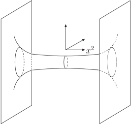
Figure 1: the shape of the D8-$\bar{D8}$-branes in the background (2.23).

We see that the configuration is deformed by the quantum effects. In classical case, we have discussed in the above section that the $N_{f}$ D8 and $N_{f}$ $\bar{D8}$-branes in this brane configuration is sit at $x^{2}=\frac{L}{2}$ and $x^{2}=-\frac{L}{2}$ respectively. And they extend to the other directions include the $U$ coordinate. They are classically not connected and the chiral symmetry $U(N_{f})_{L}\times U(N_{f})_{R}$ is not broken. But here the $N_{f}$ D8-branes and $N_{f}$ $\bar{D8}$-branes are joined into a single D8-branes by a wormhole such as in [30] and the chiral symmetry $U(N_{f})_{R}\times U(N_{f})_{L}$ is dynamically broken to a $U(N_{f})_{diag}$.

We have seen there are two brane configuration, one is the separated parallel brane configuration with fixed distance $L$, the other is the connected one by the wormhole with the minimal $U$ value $U_{0}$. We need to compare the energy density of these two configuration to see which one is preferred. The energy density difference of the two configurations is given by

$$\begin{array}[]{lll}\bigtriangleup E&\equiv E_{straight}-E_{curved}\\ &\sim\int_{0}^{U_{0}}(U-0)dU+\int_{U_{0}}^{\infty}\left(U-U(1-\frac{U_{0}^{7}}{U^{7}})^{-1/2}\right)dU\approx 0.4U_{0}^{2}\end{array}$$ (2.33)

We find the energy density difference $\bigtriangleup E$ is positive. This result means that the connected configuration by the wormhole is preferred and the chiral symmetry is likely to break.

If the above supergravity approximation is valid, the two conditions must be satisfied. One is the dilation satisfies $e^{\phi}\ll 1$, and the other is the curvature scalar that satisfied $\alpha^{\prime}R\ll 1$. Therefore the ’t Hooft coupling constant must be satisfied

$$U\ll\lambda$$ (2.34)

which is extended by the eleven-dimensional SUGRA. From (2.30), we have $U_{0}^{3}\sim\lambda/L^{2}$. And in the strong coupling region (2.3), $U_{0}$ obviously satisfies the condition (2.34). Fixing $L$ and increasing $\lambda$ will push $U_{0}$ further into the region of validity of supergravity. To the opposite direction, decreasing $\lambda$ will make $U_{0}$ become smaller, and when $L\simeq\frac{1}{\lambda}$ the curvature at $U_{0}$ becomes of order one and the supergravity description breaks down. If continuing to decrease the $\lambda$ into the region $L\ll\frac{1}{\lambda}$, the coupling becomes weak and the perturbative description is reliable as in subsection 2.1.

Until now, we have analyzed the low energy dynamics of this brane configuration in two different coupling region. In the weak coupling region (2.2), the non-local GN description of the two-dimensional dynamics is valid. And we find that the quarks get mass (2.22)and the chiral symmetry is dynamically broken. However, in the stromg coupling region, SUGRA description is reliable. We see that the energy density difference between the separated D8 and $\bar{D8}$-branes configuration and the connected D8-$\bar{D8}$-branes one by wormhole is positive. Thus the D8 and $\bar{D8}$-branes is deformed to a connected curved D8-branes that provides a geometric realization of chiral symmetry breaking. The energy scale associated with chiral symmetry breaking in the supergravity regime is $U_{0}\sim\left(\frac{\lambda}{L^{2}}\right)^{1/3}$ which can be regarded as the quark mass of $q_{L}$ and $q_{R}$ and correspond to $k^{*}\sim\sqrt{\frac{\lambda}{L}}$ in (2.22) in weak coupling region.

From the above, we know that in the one region (2.2), the field is valid, in the opposite region (2.3), the supergravity is trusted. One may ask how to get some information about the correspondence between these two sides. That means to find the correspondence between the bulk fields and the boundary operators. In below we give some superficial discussion following from [21]. We know that there are two kinds of bulk fields in this configuration. One is the massless modes of the closed string which exist even when the D8-branes are absent. The other is open string fields on the D8-branes. Both two cases are coupled to quarks $q_{L}$ and $q_{R}$. We consider first the open tachyon stretched between the D8 and $\bar{D8}$-branes. This complex scalar field which transforms as $(\bar{N_{f}},N_{f})$ under $U(N_{f})_{L}\times U(N_{f})_{R}$ couples to the fermion via Yukawa-type coupling

$${\rm{L_{1}}}\simeq Tq^{\dagger}_{R}\cdot q_{L}+\bar{T}q^{\dagger}_{L}\cdot q_{R}$$ (2.35)

Thus, the open string tachyon $T$, $\bar{T}$ is dual to the boundary operators

$$\begin{array}[]{lll}&T\leftrightarrow q^{\dagger}_{R}\cdot q_{L}\\ &\bar{T}\leftrightarrow q^{\dagger}_{L}\cdot q_{R}\end{array}$$ (2.36)

Therefore, in addition to its curved shape (2.29), the connected curved D8-brane describes a vacuum with non-zero expectation value $<q^{\dagger}_{R}\cdot q_{L}>$ will have a non-zero condensate of the $8-\bar{8}$ tachyon $T$. Another bulk field is the scalar $(X^{2})_{L}$ that parameterizes the location of the D8-branes in the direction $x^{2}$, and $(X^{2})_{R}$ for the $\bar{D8}$-branes. Unlike the tachyon, these scalars have the coupling

$${\rm{L_{2}}}\simeq(X^{2})_{L}\left(q^{\dagger}_{L}\cdot q_{R}q^{\dagger}_{R}\cdot q_{L}\right)_{(N_{f}^{2},1)}+(X^{2})_{R}\left(q^{\dagger}_{L}\cdot q_{R}q^{\dagger}_{R}\cdot q_{L}\right)_{(1,N_{f}^{2})}$$ (2.37)

The quarks coupling $\rm{L_{2}}$ don’t have interaction if the $L\rightarrow 0$. But for finite $L$, there exists interaction between quarks (2.37). In the near-horizon geometry, the coupling (2.37) implies that the bulk-boundary correspondence is

$$\begin{array}[]{lll}&(X^{2})_{L}\leftrightarrow\left(q^{\dagger}_{L}\cdot q_{R}q^{\dagger}_{R}\cdot q_{L}\right)_{(N_{f}^{2},1)}\\ &(X^{2})_{R}\leftrightarrow\left(q^{\dagger}_{L}\cdot q_{R}q^{\dagger}_{R}\cdot q_{L}\right)_{(1,N_{f}^{2})}\end{array}$$ (2.38)

The chiral symmetry breaking implies that the operators on the right-hand side of (2.38) have non-zero expectation value in our brane configuration, and which leads that the scalars $(X^{2})_{L}$, $(X^{2})_{R}$ must have a non-zero expectation value. This is the curved shape $U(x^{2})$ of the branes which is given asymptotically by (2.32). And $x^{2}$ approaches to $L/2$ as $U\rightarrow\infty$ like $L/2-x^{2}\sim U^{-5}$. One can investigate the other bulk fields to find the correspondent boundary operators. The details of the correspondence is need to further study. In this paper, we don’t expand to discuss it in details and leave to study in the future.

We now turn to give some discussions to the $8-\bar{8}$ strings in the background (2.23) as mentioned at the beginning of the section 2. As we have analyzed in the above section if the distance $L$ is smaller than the string length, the ground string mode is a tachyon, otherwise it is massive. The fundamental string is stretched between the D8 and $\bar{D8}$-branes in the near-horizon geometry of the D2-branes (2.23) and is extending in the directions $(x^{0},x^{2})$ [31, 32, 33, 21]. The induced metric on the string worldvolume is given by

$$ds^{2}=\left(\frac{U}{R}\right)^{5/2}(dx^{0})^{2}-\left({\left(\frac{U}{R}\right)^{5/2}+\left(\frac{R}{U}\right)^{5/2}\left(\frac{dU}{dx^{2}}\right)^{2}}\right)(dx^{2})^{2}$$ (2.39)

Then we can compute the fundamental string Nambu-Goto action, and it is proportional to

$$S_{NG}\sim-\int_{-L/2}^{L/2}dx^{2}\left(\frac{U}{R}\right)^{5/2}\left(1+\left(\frac{R}{U}\right)^{5}U^{\prime 2}\right)^{1/2}$$ (2.40)

where the $U^{\prime}\equiv\frac{dU}{dx^{2}}$. Since the integrand is not explicit dependent on the $x^{2}$, then the equation of motion of fundamental string is

$$\frac{d}{dx^{2}}\left(\frac{(U/R)^{5/2}}{\sqrt{1+\left(\frac{R}{U}\right)^{5}U^{\prime 2}}}\right)=0$$ (2.41)

If we choose the boundary conditions, $U^{\prime}(x^{2})=0$ and $U=U_{0}^{F}$ at $x^{2}=0$, and $x^{2}=\pm\frac{L}{2}$ if the $U\rightarrow\infty$. Then the first order equation is

$$\frac{(U/R)^{5/2}}{\sqrt{1+\left(\frac{R}{U}\right)^{5}U^{\prime 2}}}=(U_{0}^{F}/R)^{5/2}$$ (2.42)

We have noted that the $U_{0}^{F}$ is the minimal value of U. From (2.42) and changing the integral variable, the equation becomes the integral form

$$\begin{array}[]{lll}x^{2}(U)&=\int_{U_{0}^{F}}^{U}\frac{dU}{(\frac{U}{R})^{5/2}\left(\left(\frac{U}{U_{0}^{F}}\right)^{5}-1\right)^{1/2}}\\ &=\frac{R^{5/2}}{(U_{0}^{F})^{3/2}}\int_{1}^{\frac{U}{U_{0}^{F}}}dxx^{-5/2}(x^{5}-1)^{-1/2}\end{array}$$ (2.43)

For the large U, this means that U is larger than $U_{0}^{F}$, so the upper limit of the integral (2.43) can be taken to infinity. Then the result of the integral is

$$x^{2}(U)=\frac{R^{5/2}}{5(U_{0}^{F})^{3/2}}\left(B(\frac{4}{5},\frac{1}{2})-B(\left(\frac{U_{0}^{F}}{U}\right)^{5},\frac{4}{5},\frac{1}{2})\right)$$ (2.44)

This means the distance $\frac{L}{2}=\frac{R^{5/2}}{5(U_{0}^{F})^{3/2}}B(\frac{4}{5},\frac{1}{2})$. For the large $U$, the curve shape of the fundamental string in this background is described by

$$U^{4}\simeq\frac{(U_{0}^{F})^{5/2}R^{5/2}}{4(\frac{L}{2}-x^{2}(U))}$$ (2.45)

Also we can compare the minima value of $U$ for the fundamental string and D8-brane that is

$$\frac{U_{0}^{F}}{U_{0}}=\frac{7B(\frac{4}{5},\frac{1}{2})}{5B(\frac{5}{7},\frac{1}{2})}\approx 1.4$$ (2.46)

Thus the minimal $U$ value of the fundamental string is larger than the correspondent one of D8-brane and stays a short distance with the minimal value $U_{0}$ of D8-branes. This picture is same as in [21]. We can compare the length of curved fundamental string with the straight one. The length of curved is proportional to

$$L_{curved}\sim\int_{1}^{x}\frac{dxx^{5/4}}{\sqrt{x^{5}-1}}$$ (2.47)

and the straight one is

$$L_{straight}\sim\int_{1}^{x}\frac{dx}{x^{5/2}\sqrt{x^{5}-1}}$$ (2.48)

Where the $x\equiv\frac{U}{U_{0}^{F}}$. And then the behavior of the compared value $\frac{L_{curved}}{L_{straight}}$ is shown in the figure 2. With increasing the value of $U$, the compared value will become large. And the tachyon mode becomes massive and decoupled. Under ours definition (2.47) and (2.48), we find the behavior is different to the case of the fundamental string in the near horizon geometry of $N_{c}$ D4-branes in [21].

Figure 2: the behavior of the length of curved string compared with the straight one in background (2.23).

3 A generalization of D-brane configuration

In this section, just as did in [4, 12, 21], we generalize the brane configuration of last section by wrapping the one direction $x^{2}$ of D2-brane on a circle of radius $R_{2}$ with antiperiodic boundary conditions for the fermion on the D2-branes worldvolume. The antiperiodic boundary conditions break all the susy, and the mass of the adjoint fermions and scalars are in general produced via at tree level and one loop, respectively [34]. As discussed in section 2, the trace parts of the scalar fields $A_{2}$ and $\phi^{i}(i=3,\cdots,9)$ is still massless by shift symmetry. However, since they can only couple to the other massless modes through irrelevant operators, and they are not important in the low energy theory. Below the mass of the fermions and scalars, the only dynamical degree of freedom are $U(N_{c})$ gauge fields and $N_{f}$ fermions in the fundamental representation of the gauge group $U(N_{c})$ as showed in section 2. We think the low energy effective theory on two dimension is $QCD_{2}$ [35]. But because of an infinite tower of Kaluza-Klein modes of mass scale $M_{KK}(M_{KK}\sim 1/R_{2})$, at high energy the low energy dynamics of this configuration can’t be described by $QCD_{2}$ .

As in the previous section, we can analyze the coupling parameter space. But in this case one more scale parameter, the radius $R_{2}$ of a circle for the $x^{2}$ direction, is introduced by the compactified D2 branes. If the radius $R_{2}$ approaches infinite, it can go back to the original brane configuration. We now will begin to discuss the coupling parameter space. Firstly, in the region

$$l_{s}\ll L\ll R_{2}\ll\frac{1}{\lambda}$$ (3.1)

the ’t Hooft coupling constant is small, and the low energy dynamics on the D2-branes is weakly coupled. The compactified radius $R_{2}$ is finite and the two-dimensional ’t Hooft coupling constant $\lambda_{2}=\frac{\lambda}{2\pi R_{2}}$ is also small, since the effective coupling constant $g_{eff}\sim L^{2}/(\frac{2\pi R_{2}}{\lambda})\ll 1$. Therefore, in this region the two-dimensional theory is also weak coupled, and we can use the usual $QCD_{2}$ techniques to study this theory. Similar to the discussions [21], for small $\lambda_{2}$, since the scale $\Lambda_{QCD_{2}}$ is much smaller than the dynamically generated quark mass $k^{*}\sim\sqrt{\lambda/L}$, the low energy theory can separate into two essentially decoupled parts. The one at distance scale $1/k^{*}$ is a chiral symmetry breaking part that is described by the non-local GN model as in section two. The second one is a confining part at the distance $1/\Lambda_{QCD_{2}}$.

With increasing the ’t Hooft coupling constant, the parameter relation becomes

$$l_{s}\ll L\ll\frac{1}{\lambda}\ll R_{2}$$ (3.2)

We find the three dimensional effective coupling constant $g_{eff}\sim L\lambda)\ll 1$, so the theory is weakly coupled. And the two dimensional effective coupling constant is still $L^{2}/(\frac{2\pi R_{2}}{\lambda})\ll 1$. As in region (3.1), the three-dimensional and two-dimensional coupling are both weak, thus we can use the perturbative analysis.

Further increasing $\lambda$, the coupling parameter relation reaches

$$\frac{1}{\lambda}\ll l_{s}\ll L\ll R_{2}$$ (3.3)

The ’t Hooft coupling $\lambda$ is large while the two dimensional effective coupling constant $g_{eff}\sim L^{2}/(2\pi R_{2}/\lambda)$ can be smaller or larger than one. If $L\lambda)\gg R_{2}/L$, then the effective coupling, $g_{eff}\ll 1$, in this case the three-dimensional dynamics must be described by SUGRA as in section 2.2, however the two-dimensional one is still described by $QCD_{2}$. In the opposite case, $g_{eff}\gg 1$, both the three-dimensional and two-dimensional dynamics are strong coupling, thus we must use the supergravity to study both the chiral symmetry breaking and confinement.

In the following, we focus on the strong coupling region both the two and three dimensional couplings. In this case, the supergravity is trusted. As the same argument in [4], if compactifying the one direction $x^{2}$ on a circle of radius $R_{2}$ with antiperiodic boundary conditions for the fermions living on the D2-branes worldvolume. we find that the near-horizon geometry metric of the D2-branes is

$$ds^{2}=\left(\frac{U}{R}\right)^{5/2}(-(dx^{0})^{2}+(dx^{1})^{2}+f(U)(dx^{2})^{2})+\left(\frac{R}{U}\right)^{5/2}(\frac{dU^{2}}{f(U)}+U^{2}d\Omega_{6}^{2})$$ (3.4)

$$e^{\phi}=\left(\frac{6\pi^{2}N_{c}g_{3}^{10}}{U^{5}}\right)^{1/4},~{}~{}~{}f(U)=1-\left(\frac{U_{KK}}{U}\right)^{5}$$ (3.5)

where we set the $\alpha^{\prime}\equiv 1$, the $R^{5}\equiv 6\pi^{2}N_{c}g_{3}^{2}$ and the constant parameter $U_{KK}$. In order to avoid a singularity at $U=U_{KK}$, the $x^{2}$ must be a periodic variable with

$$x^{2}\sim x^{2}+\delta x^{2},~{}~{}~{}~{}\delta x^{2}=\frac{4\pi R^{5/2}}{5U_{KK}^{3/2}}$$ (3.6)

we can define the Kaluza-Klein mass as

$$M_{KK}\sim\frac{1}{R_{2}}=\frac{2\pi}{\delta x^{2}}=\frac{5U_{KK}^{3/2}}{2R^{5/2}}$$ (3.7)

Then the parameter constant $U_{KK}$ satisfied

$$U_{KK}^{3}=\frac{24\pi^{2}\lambda}{25R_{2}^{2}}$$ (3.8)

The $U$ coordinate is restricted to $U\geq U_{KK}$ in order to finite volume of $S^{6}$ and warp factor of $R^{1,1}$. And for $U_{0}$ it is also larger than $U_{KK}$, which can see from the equation (3.3), (3.8) and $U_{0}\sim(\lambda/L^{2})^{1/3}$.

We now will consider a probe D8-brane propagating in this metric background. The D8-brane is extended in the directions $R^{1,1}\times R\times S^{6}$, and we are interested in the solution $x^{2}(U)$ in the coordinates plane $(x^{2},U)$. The induced metric on the D8-brane is

$$\begin{array}[]{lll}ds^{2}&=\left(\frac{U}{R}\right)^{5/2}(-(dx^{0})^{2}+(dx^{1})^{2})\\ &+\left(\left(\frac{U}{R}\right)^{5/2}f(U)\left(\frac{dx^{2}}{dU}\right)^{2}+\frac{1}{f(U)}\left(\frac{R}{U}\right)^{5/2}\right)dU^{2}+\left(\frac{R}{U}\right)^{5/2}U^{2}d\Omega_{6}^{2}\end{array}$$ (3.9)

From the induced metric (3.9), we get the DBI action of the D8-brane

$$S_{D8}\sim\int dx^{2}U\sqrt{\left(\frac{U}{R}\right)^{5}f(U)+\frac{U^{\prime 2}}{f(U)}}$$ (3.10)

where the $U^{\prime}=\frac{dU}{dx^{2}}$. Since the integrand of (3.10) does not explicitly depend on $x^{2}$, we can obtain the equation of motion as the energy conservation law

$$\frac{d}{dx^{2}}\left(\frac{U^{6}f(U)}{\sqrt{\left(\frac{U}{R}\right)^{5}f(U)+\frac{U^{\prime 2}}{f(U)}}}\right)=0$$ (3.11)

Assuming the initial conditions $U(0)=U_{0}$ and $U^{\prime}(0)=0$ at $x^{2}=0$, the solution of this equation of motion is obtained as

$$x^{2}(U)=U_{0}^{7/2}f(U_{0})^{1/2}\int_{U_{0}}^{U}\frac{dU}{\left(\frac{U}{R}\right)^{5/2}f(U)\sqrt{U^{7}f(U)-U_{0}^{7}f(U_{0})}}$$ (3.12)

For the approximation $U\gg U_{0}$, the integral (3.12) can integrate from $U_{0}$ to $\infty$, and $x^{2}(\infty)=L/2$. If $U_{0}=U_{KK}$, then the $x^{2}(\infty)\approx\frac{R^{5/2}}{5U_{0}^{3/2}}\sim\delta x^{2}$. In this case, it means the $L\sim R_{2}$, and the D8-brane and the $\bar{D8}$-brane are at antipodal points on the $S^{1}$ circle of the $x^{2}$ direction. If $U_{0}\rightarrow\infty$, then the D8 and $\bar{D8}$-branes approaches to infinity and disappears. The distance $\frac{L}{2}=x^{2}(\infty)$ is a monotonically decreasing function of $U_{0}$. It has some similar to the fundamental string stretched between the D8 and $\bar{D8}$-branes in the unwrapping near-horizon D4-branes background that the length of fundamental string is a monotonically decreasing function of $U$ but not $U_{0}$. In this background, the D8-branes and $\bar{D8}$-branes join together at the minimal value $U=U_{0}$ through wormhole and the chiral symmetry is broken. It can be shown as the way in section 2.2. we can also understand it since there is the attractive force between the D8 and $\bar{D8}$-branes, thus the D8-branes and $\bar{D8}$-branes connected form is preferred than the separated case.

As in the subsection 2.2, we can study the fundamental string stretched between the D8 and $\bar{D8}$-branes in the background (3.4) and (3.5). Assuming the fundamental string extends in the $(x^{0},x^{2})$ directions. We are only interested in the string shape in the $(x^{2},U)$ directions, then the induced metric of the fundamental string is

$$ds^{2}=-\left(\frac{U}{R}\right)^{5/2}(dx^{0})^{2}+\left(\left(\frac{U}{R}\right)^{5/2}f(U)+\frac{1}{f(U)}\left(\frac{R}{U}\right)^{5/2}\left(\frac{dU}{dx^{2}}\right)^{2}\right)(dx^{2})^{2}$$ (3.13)

then substituting into the Nambu-Goto action of string, we can get

$$S_{NG}\sim\int dx^{2}\left(\left(\frac{U}{R}\right)^{5}f(U)+\frac{U^{\prime 2}}{f(U)}\right)^{1/2}$$ (3.14)

with the $U^{\prime}=\frac{dU}{dx^{2}}$. With boundary condition $U(0)=U_{0}^{F_{1}}$ and $U^{\prime}(0)=0$, the $U(x^{2})$ satisfies the first order equation

$$\frac{U^{5/2}f(U)^{1/2}}{\sqrt{1+\left(\frac{R}{U}\right)^{5}\frac{U^{\prime 2}}{f(U)^{2}}}}=(U_{0}^{F_{1}})^{5/2}f(U_{0}^{F_{1}})^{1/2}$$ (3.15)

Here the $U_{0}^{F_{1}}$ is the minimal value of $U$ that corresponds to the $U_{0}^{F}$ of the fundamental string in the background (2.23) in section 2.2. We can solve the $x^{2}(U)$ as follows

$$x^{2}(U)=(U_{0}^{F_{1}}R)^{5/2}f(U_{0}^{F_{1}})^{1/2}\int_{U_{0}^{F_{1}}}^{U}\frac{dU}{U^{5/2}f(U)\sqrt{U^{5}f(U)-(U_{0}^{F_{1}})^{5}f(U_{0}^{F_{1}})}}$$ (3.16)

For the $U$ larger than the $U_{0}^{F_{1}}$ so that the upper limit of the integral (3.16) can be taken to infinity and can define the $\frac{L}{2}=x^{2}(\infty)$. From the integral (3.16), if $U_{0}=U_{KK}$, we get

$$\frac{L}{2}=x^{2}(\infty)\approx\frac{R^{5/2}}{4(U_{0}^{F_{1}})^{3/2}}$$ (3.17)

Now we compare the minimal value of $U$ for the fundamental string and the D8-brane. It is

$$\frac{U_{0}^{F_{1}}}{U_{0}}\approx\frac{5}{4}$$ (3.18)

Hence approximately we can obtain the $U_{0}^{F_{1}}$ is larger than $U_{0}$ as same as in (2.46). If the $U_{0}\rightarrow\infty$, then the fundamental string runs and disappears to infinity.

We can also discuss the meson spectrum in this configuration as in [12]. To study the fluctuation modes around the D8-branes, we can determine the degrees of freedom corresponding to the massless particles. In the paper [38], the authors give some discussion about the meson spectrum of this model.

Until now, the all above discussion is at zero temperature. In the following we turn to study the theory in the strong ’t Hooft coupling region and at a finite temperature. We do a analytically continue the time coordinate $x^{0}\rightarrow x^{0}_{E}=ix^{0}$ with period $T,~{}~{}x^{0}_{E}\approx x^{0}_{E}+T$, and impose antiperiodic boundary conditions on the fermions in the direction $x^{0}_{E}$ [4]. Then there are two Euclidean supergravity solutions which need to considered that it is same as the D4-branes [11, 36]. The first one is

$$ds^{2}=\left(\frac{U}{R}\right)^{5/2}((dx^{0}_{E})^{2}+(dx^{1})^{2}+f(U)(dx^{2})^{2})+\left(\frac{R}{U}\right)^{5/2}(\frac{dU^{2}}{f(U)}+U^{2}d\Omega_{6}^{2})$$ (3.19)

which is obvious the Euclideanised version of metric (3.4). And from the black D2-branes, the second metric can be written as

$$ds^{2}=\left(\frac{U}{R}\right)^{5/2}(\tilde{f}(U)(dx^{0}_{E})^{2}+(dx^{1})^{2}+(dx^{2})^{2})+\left(\frac{R}{U}\right)^{5/2}(\frac{dU^{2}}{\tilde{f}(U)}+U^{2}d\Omega_{6}^{2})$$ (3.20)

where the $\tilde{f}(U)=1-\left(\frac{U_{T}}{U}\right)^{5}$. These two metric are equal to each other after commuting $x^{0}_{E}$ with $x^{2}$ and $U_{KK}$ with $U_{T}$. To avoid the singularity of the metrics at $U=U_{KK}$ and $U_{T}$, the coordinates must satisfy the periodic boundary conditions. Then the periodicity of $\delta x^{2}$ in (3.19) satisfies (3.6), and in (3.20) the periodicity of $x^{0}_{E}$ is $\delta x^{0}_{E}=\frac{4\pi R^{5/2}}{5U_{T}^{3/2}}$. However, the periodicity of the other two coordinates is arbitrary. Hence, the temperature of background (3.19) is arbitrary, the second one is proportional to the inverse of $\delta x^{0}_{E}$. At a given temperature, we need to decide which background dominates the path integral. We can compare the free energies of these two backgrounds and see which one has a lower free energy. There is a critical temperature $T^{*}$, under it, the background (3.19) dominates the path integral. Otherwise, if the temperature is higher than the critical temperature $T^{*}$, the metric (3.20) dominates. From the low temperature to the high energy temperature, there is a Hawking-Page phase transition between them [37].

In the low temperature phase, the analysis is same as the zero temperature case except that the time is Euclidean and compactified with a circumference $\frac{1}{T}$, where $T$ is the temperature. We can use the dual description and find the chiral condensate as in the zero temperature case. The equation of motion of D8-brane in this background is similar to the equation (3.12). We can find that the configuration of the D8-branes and $\bar{D8}$-branes are connected each other in this background. It hints the chiral symmetry breaking in the dual gauge theory.

However, in the high temperature phase, the background (3.20) dominates the path integral. As done in the zero temperature, we use the D8-brane to probe the background and find the dynamical curve in the plane $(x^{2},U)$. Here we assume that the D8-brane extends in directions $(x^{0}_{E},x^{1},U,\Omega_{6})$, the induced metric on the D8-brane is

$$\begin{array}[]{lll}ds^{2}&=\left(\frac{U}{R}\right)^{5/2}(\tilde{f}(U)(dx^{0}_{E})^{2}+(dx^{1})^{2})\\ &+\left(\left(\frac{U}{R}\right)^{5/2}\left(\frac{dx^{2}}{dU}\right)^{2}+\frac{1}{\tilde{f}(U)}\left(\frac{R}{U}\right)^{5/2}\right)dU^{2}+\left(\frac{R}{U}\right)^{5/2}U^{2}d\Omega_{6}^{2}\end{array}$$ (3.21)

Then using the dilaton (3.5) and induced metric (3.21) and neglecting some proportional constant, the DBI action is

$$S\sim\int dx^{2}U\sqrt{\left(\frac{U}{R}\right)^{5}\tilde{f}(U)+U^{\prime 2}}$$ (3.22)

where the $U^{\prime}=\frac{dU}{dx^{2}}$. Obviously, this equation will reduce to equation (2.26) if $\tilde{f}(U)=1$, i.e. $U_{T}=0$. From the above action (3.22), we can get the equation of motion

$$\left(\frac{d}{dx^{2}}\right)\left(\frac{U^{6}\tilde{f}(U)}{\sqrt{\left(\frac{U}{R}\right)^{5}\tilde{f}(U)+U^{\prime 2}}}\right)=0$$ (3.23)

If we set the boundary condition of the above equation as $U(x^{2})=U_{0}$ and $U^{\prime}(x^{2})=0$, then we obtain the first order equation

$$\frac{U^{7/2}\tilde{f}(U)^{1/2}}{\sqrt{1+\left(\frac{R}{U}\right)^{5}\frac{U^{\prime 2}}{\tilde{f}(U)}}}=U_{0}^{7/2}\tilde{f}(U_{0})^{1/2}$$ (3.24)

Then the curve $x^{2}(U)$ can be expressed as

$$x^{2}(U)=\int_{U_{0}}^{U}\frac{dU}{\tilde{f}(U)^{1/2}\left(\frac{U}{R}\right)^{5/2}\sqrt{\left(\frac{U}{U_{0}}\right)^{5}\frac{\tilde{f}(U)}{\tilde{f}(U_{0})}-1}}$$ (3.25)

The value $U_{0}$ at $x^{2}=0$ is the smallest value of $U$ where the D8-branes are connected with the $\bar{D8}$-branes. When the minimal value $U_{0}$ of the D8-brane shape $U(x^{2})$, $U_{0}\rightarrow U_{T}$, then the D8-brane approaches to the horizon of the black hole. If $U_{0}$ reaches to the value $U_{T}$, this means that the wormhole of the connected D8-$\bar{D8}$-brane pairs reaches the horizon of this black hole background. However, if the $U_{0}\rightarrow\infty$, then the D8-$\bar{D8}$-brane pairs approach to infinity and disappear.

Substituting the equation (3.25) into the DBI action (3.22) and using the integral variable $y\equiv\frac{U}{U_{0}}$, we get the

$$S_{1}\sim\int_{1}^{\infty}dy\frac{y}{\sqrt{1-\frac{\tilde{f}(1)}{\tilde{f}(y)y^{7}}}}$$ (3.26)

For the D8 and $\bar{D8}$-branes separated case, we also can get

$$S_{2}\sim\int_{y_{T}}^{1}dyy+\int_{1}^{\infty}dyy$$ (3.27)

To determine whether the chiral symmetry is broken or not in high temperature. We now need to compare the free energy of this configuration with the energy of the separated D8-branes and $\bar{D8}$-branes configuration. Since the D8-branes extend to infinity, thus the energy is divergent. But the difference between these two configurations is finite. Then from the equation (3.26) and (3.27), the difference energy is proportional to

$$\delta S=S_{1}-S_{2}=\int_{1}^{\infty}dyy\left(\frac{1}{\sqrt{1-\frac{\tilde{f}(1)}{\tilde{f}(y)y^{7}}}}-1\right)-\int_{y_{T}}^{1}dyy$$ (3.28)

if we define the $z\equiv y^{-7}$, then the $\delta S$ can be written as

$$\delta S=\frac{1}{7}\int_{0}^{1}dzz^{-9/7}\left(\frac{\sqrt{1-y_{T}^{5}z^{5/7}}}{\sqrt{1-y_{T}^{5}z^{5/7}-(1-y_{T}^{5})z}}-1\right)-\frac{1}{2}(1-y_{T}^{2})$$ (3.29)

Then we can use a numerical way to analyze the integral and draw a Fig. 3 in the following

Figure 3: the relations between the energy difference $\delta$S and $y_{T}$.

In the following, we can see, in the high temperature phase $T>\frac{1}{2\pi R_{2}}$ which is dominated by the background (3.20), there exists a first order phase transition of the chiral symmetry breaking. From the figure 3, there is a critical point $y_{T}\sim 0.80$ where $\delta S=0$. By increasing the $y_{T}$, if the $y_{T}$ is larger than a critical value $y_{T}\sim 0.80$, then the energy difference $\delta S$ is positive. Thus the preferred branes configuration is the disconnected D8 and $\bar{D8}$-branes case. It means that the chiral symmetry is unbroken in this region. Otherwise, in the region $y_{T}<0.80$, the configuration of the connected D8 and $\bar{D8}$-branes is preferred, in this case the chiral symmetry is broken. Therefore, we know that at the critical point $y_{T}\sim 0.80$, there is a first order phase transition of the chiral symmetry breaking. The results in here is very similar to the case in SS model at finite temperature that is analyzed by [15, 16]. In the SS model, there also exists a critical temperature. And above this temperature, the chiral symmetry is unbroken. However, under it, the symmetry is broken.

In the equation (3.25), if approximately choosing the $U$ larger than the $U_{0}$, then the upper limit of the integral can be leaded to infinity. The asymptotic distance $L$ between D8-branes and $\bar{D8}$-branes is equal to

$$\frac{L}{2}=R^{5/2}\int_{U_{0}}^{\infty}\frac{dU}{\tilde{f}(U)^{1/2}U^{5/2}\sqrt{\left(\frac{U}{U_{0}}\right)^{7}\frac{\tilde{f}(U)}{\tilde{f}(U_{0})}-1}}$$ (3.30)

After a change of the integral variable, the above equation (3.30) becomes

$$\begin{array}[]{lll}\frac{L}{2}=&U_{0}^{-3/2}R^{5/2}\int_{1}^{\infty}\frac{dy}{\tilde{f}(y)^{1/2}y^{5/2}\sqrt{\frac{\tilde{f}(y)}{\tilde{f}(1)}y^{7}-1}}\\ &=\frac{1}{7}U_{0}^{-3/2}R^{5/2}\sqrt{1-y_{T}^{5}}\int_{0}^{1}\frac{dz}{z^{2/7}(1-y_{T}^{5}z^{5/7})^{1/2}\sqrt{1-y_{T}^{5}z^{5/7}-(1-y_{T}^{5})z}}\end{array}$$ (3.31)

If the $y_{T}\ll 1$, the $U_{0}$ has the relation $U_{0}^{3}\sim R^{5}/L^{2}$. This means that the $L\rightarrow 0$ with increasing the $U_{0}$, and the D8-$\bar{D8}$-branes will run to infinity and disappear. When the $y_{T}\rightarrow 1$, then the D8-$\bar{D8}$-branes throat will run to the horizon of the black hole background (3.20) and eventually meet each other. If we choose that the $y_{T}$ is equal to the critical point of the phase transition of the chiral symmetry. From the integral (3.31), we get the correspondent value $L\simeq 0.33\frac{R^{5/2}}{U_{0}^{3/2}}$ at this critical temperature. Using the period condition $\delta x^{0}_{E}=\frac{4\pi R^{5/2}}{5U_{T}^{3/2}}$, we get the relation about the temperature $T$ with the asymptotic distance $L$ at this critical point, and that is $T^{\chi}\simeq\frac{0.09}{L}$. We know that there is a Hawking-Page transition from the low temperature (3.19) to the high temperature (3.20). And we can set that the critical temperature of Hawking-Page phase transition is $T^{*}=\frac{1}{2\pi R_{2}}$. If the $L>0.57R_{2}$, then the temperature in this deconfined phase is always higher than $T^{\chi}$, thus the deconfinement and chiral symmetry restoration happen together. On the opposite side $L<0.57R_{2}$, It means that the theory lies in the deconfinement phase and the deconfinement and chiral symmetry restoration transitions happen separated.

We have studied the zero and finite temperature case of this D2-D8-$\bar{D8}$-branes configuration. In the following we give some discussions about the relations of this branes system with others D-branes configuration. After performing a T-dual to this D-branes configuration along the direction $x^{2}$, we can get a D1-D9-$\bar{D9}$-branes configuration in the IIB string theory. This configuration has been studied in [26]. In this D1-D9-$\bar{D9}$-branes configuration the D1, D9 and $\bar{D9}$-branes are parallel each other. As in the section 2, we can analyze the massless degrees of freedom on the D-branes. If choosing the color index $N_{c}=1$, the low energy dynamics on the D1-brane is a two-dimensional massless QED(Schwinger model) which is exactly solvable. This theory is equivalent to a free massive scalar field theory by using the bosonization techniques. For the bulk tachyon modes of the 9-$\bar{9}$-string, the tachyon fields will couple to the fermions on the D1-brane via Yukawa coupling and the fermions get mass. Then the dynamics on the D1-brane is a massive two-dimensional QED, it is no longer a solvable theory. But we can still use the bosonization way to study it. When the tachyon fields get large vacuum expectation value, the Yukawa coupling between the bulk tachyon and the worldvolume fermions of D1-brane is decoupled from the low energy physics, and the massive two-dimensional QED will reduce to the massless two-dimensional QED. Also if compactifying one longitudinal direction of the D1-brane on a circle and performing a duality again along this compacted direction, we get the D0-D8-$\bar{D8}$-branes configuration. The D0-branes in D8-$\bar{D8}$-branes background can be described by the Matrix-theory [26]. The other brane system such as D2-D6-$\bar{D6}$ and D2-D4-$\bar{D4}$ brane configurations, they also have two intersectional dimensions In these brane configurations [38] as the D2-D8-$\bar{D8}$ brane configuration. One can use the same way to study these brane configurations as the D2-D8-$\bar{D8}$ brane configuration in this paper.

4 summaries

Motivated by the ads/cft, much work has been done to give a holographic dual description of the large $N_{c}$ QCD with flavors by string theory such as [8, 11, 12]. In this paper, we construct a two-dimensional toy model from the D2-D8-$\bar{D8}$-branes configuration in IIA string theory. In section 2, we analyze the massless spectrum on the two-dimensional intersection of this branes configuration and show them in the table 1. In the weak coupling region $l_{s}\ll L\ll\frac{1}{\lambda}$, the low energy dynamics on the intersection is a non-local GN model. We know that the GN model is asymptotically free and exactly solvable at large $N_{c}$ and finite $N_{f}$ and dynamical breaks the chiral flavor symmetry $U(N_{f})_{L}\times U(N_{f})_{R}$. The non-local GN model is a non-local generalization of the GN model, it can be seen from the equation (2.7). Using this NGN model, we find the quarks condensate and the chiral symmetry breaking. But in the opposite coupling region (2.3), the interaction becomes strong and we can’t use the perturbative way to study the low energy dynamics of this brane system. Instead the IR dynamics can be described by the SUGRA approximation. We find the connected D8-$\bar{D8}$-branes configuration by the wormhole is preferred. And it means that the chiral symmetry is broken. This gives a geometric realization of the chiral symmetry breaking. In both the descriptions, we find the chiral symmetry is dynamically broken. We also discuss some bulk and boundary correspondences of this brane configuration, however, the details of the correspondences is needed to further study. For the fundamental string in the background (2.23), we find some interesting results. From the equation (2.46), we can see that the minimal value $U_{0}^{F}$ of the fundamental string is always larger than the correspondence one of the D8-$\bar{D8}$-branes in this background. It means that the fundamental strings don’t reach the minimal value $U_{0}$ of D8-branes and stay a short distance away from it. Also we have compared the strength between the curved and the straight fundamental string. We find the curved string is longer than the straight one.

In the section 3, we give a generalization of the D-branes configuration. It can be got through wrapping one direction $x^{2}$ of the D2-brane on a circle of radius $R_{2}$ with anti-periodic condition of the fermions. Then the fermions and scalars get mass and decouple from the IR physics. The only massless modes on D2-branes are the quarks and gauge fields. In the weak coupling region $l_{s}\ll L\ll R_{2}\ll\frac{1}{\lambda}$, the low energy two dimensional physics can be described by the $QCD_{2}$. We can use the standard techniques to study this theory. However, in the opposite region $\frac{1}{\lambda}\ll l_{s}\ll L\ll R_{2}$, the interaction becomes strong. And instead the perturbative analysis, the SUGRA can be used to describe this region and we can find the chiral symmetry is dynamically broken as in the section 2. Following [12], the meson spectrum of this model need to work out. In [38], there are some discussions about the meson spectrum of this model.

In the following we also study the properties of this system at finite temperature. At low temperature, the metric (3.19) determines the path integral. However, at high temperature, the background (3.20) determines. We know that with the increasing temperature there happens a Hawking-Page deconfinement phase transition from the background (3.19) to (3.20). At the high temperature phase, there is a chiral symmetry phase transition critical point $y_{T}=0.80$ or $T^{\chi}=\frac{0.09}{L}$. Below this point, the chiral symmetry is broken. However, up this point, the chiral symmetry is restored. In the last, we have discussed some relations about this configuration with the other branes configuration. For example the D1-D9-$\bar{D9}$-branes configuration, the low energy dynamics on one D1-brane is two-dimensional QED. If performing the T-duality again along the D1-branes worldvolume, the brane configuration becomes the D0-D8-$\bar{D8}$ brane system and the D0-branes dynamics have a matrix description. There are some other D-brane configurations such as D2-D6-$\bar{D6}$ and D2-D4-$\bar{D4}$ which also exist two dimensional intersection. For these brane system, we can perform the same analysis as the D2-D8-$\bar{D8}$ brane configuration in this paper.

Acknowledgements
W. Xu would like to thank K. Ke, M.X. Luo and H.X. Yang for reading the manuscript and giving many suggestions, and L.M. Cao, D.W. Pang, J.H. She, J.P. Shock, X. Su and Z. Wei for some useful helps and nice discussions.

References

- [1] J.Maldacena, “The Large N Limit Of Superconformal Field Theories And Supergravity,” hep-th/9711200; S.S.Gubser, I.R.Klebnov and A.M.Polyakov,“ Gauge Theory Correlators From Noncritical String Theory,” hep-th/9802109; E.Witten,“ Anti-de Sitter Space And Holography,” hep-th/9802150.
- [2] David Berenstein, Juan M. Maldacena, Horatiu Nastase , “Strings in flat space and pp waves from N=4 superYang-Mills” JHEP 0204:013,2002 ; hep-th/0202021.
- [3] O.Aharony, S.S.Gubser, J.M.Maldacena, H.Ooguri and Y.Oz, “Large-N Field Theories, String Theory and Gravity,” Phys.Rep.323(2000)183; hep-th/9905111.
- [4] E.Witten, “Anti-de Sitter space , thermal phase transition, and confinement in gauge theories,” Adv.Theor.Math.Phys.2(1998)505;hep-th/9803131.
- [5] J.Polchinski and M.J.Strassler, “The String Dual Of A Confining Four-Dimensional Gauge Theory,” hep-th/0003136.
- [6] I.R.Klebanov and M.J.Strassler, “Supergravity and A Confining Guage Theory: Duality Cascades and ChiSB-Resolution of Naked Singularties,” J.High Energy Phys.0008,052(2000); hep-th/0007191.
- [7] J.M.Maldacena and C.Nunez, “Towards the Large N Limit of Pure N=1 Super Yang-Mills,” Phys.Rev.Lett.86,588(2001); hep-th/0008001.
- [8] A.Karch and E.Katz,“Adding Flavor to Ads/Cft,” J.High Energy Phys.06(2002)043; hep-th/0205236.
- [9] T.Sakai and S.Sugimoto,“Probing flavored Mesons of Confining Gauge Theories by Supergravity,” J.High Energy Phys.0309,047(2003); hep-th/0305049.
- [10] J.Babington, J.Erdmenger, N.J.Evans, Z.Guralnik and I.Kirsch, “Chiral Symmetry Breaking and Pions in Non-supersymmetric Gauge/Gravity Duals,” Phys.Rev.D69,066007(2004), hep-th/0306018; Nick J. Evans, Jonathan P. Shock, “Chiral dynamics from AdS space,”hep-th/0403279; Nick Evans, Jon Shock, Tom Waterson,“D7 brane embeddings and chiral symmetry breaking,” hep-th/0502091; Jonathan P. Shock ,“Canonical coordinates and meson spectra for scalar deformed N=4 SYM from the AdS/CFT correspondence,” hep-th/0601025; D. Arean and A.V. Ramallo, “Open String modes at brane intersections,” J. High Energy Physics 0604 (2006) 037, hep-th/0602174.
- [11] M.Kruczenski, D.Mateos, R.C.Myers and D.J.Winters, “Towards a Holographic Dual of Large-Nc QCD,” J.High Energy Phys. 05(2004)041;hep-th/0311270.
- [12] T.Sakai and S.Sugimoto,“Low Energy Hadron Physics in Holographic QCD,” hep-th/0412141
- [13] T.Sakai and S.Sugimoto,“More on A Holographic QCD,” hep-th/0507073.
- [14] Robert C. Myers, Rowan M. Thomson,“Holographic Mesons in Various Dimensions,” hep-th/0605017.
- [15] Ofer Aharony, Jacob Sonnenschein, Shimon Yankielowicz,“A Holographic Model of Deconfinement and Chiral Symmetry Restoration,” hep-th/0604161 .
- [16] Andrei Parnachev, David A. Sahakyan,“Chiral Phase Transition from String Theory,” hep-th/0604173.
- [17] David Mateos, Robert C. Myers, Rowan M. Thomson,“Holographic Phase Transitions with Fundamental Matter,” hep-th/0605046.
- [18] Paolo Benincasa, Alex Buchel,“Hydrodynamics of Sakai-Sugimoto model in the quenched approximation ”, hep-th/0605076.
- [19] Tameem Albash, Veselin Filev, Clifford V. Johnson, Arnab Kundu,“A Topology-Changing Phase Transition and the Dynamics of Flavour,” hep-th/0605088.
- [20] Andreas Karch, Andy O’Bannon, “ Chiral Transition of N=4 Super Yang-Mills with Flavor on a 3-Sphere ,” hep-th/0605120.
- [21] E. Antonyan, J.A. Harvey, S. Jensen, D. Kutasov,“NJL and QCD from String Theory,” hep-th/0604017.
- [22] Y.Nambu and G.Jona-Lasinio, “Dynamical Model of Elementary Particles Based on An Analogy with Superconductivity.I,” Phys.Rev.122,345(1961).
- [23] D.J.Gross and A.Neveu, “Dynamical Symmetry Breaking In Asymptotically Free Field Theories,” Phys.Rev.D10,3235(1974).
- [24] M.Moshe and J.Zinn-Justin, “Quantum Field Theory in The Large N Limit: A Review,” Phys.Rept.385,69(2003); hep-th/0306133.
- [25] Sidney R. Coleman, E. Weinberg, “Radiative Corrections As The Origin Of Spontaneous Symmetry Breaking,” Phys.Rev.D7:1888-1910,1973
- [26] S.Sugimoto and K.Takahashi,“QED and String Theory,” hep-th/0403247
- [27] Julian S. Schwinger, “Gauge Invariance And Mass,” Phys.Rev.125:397-398,1962; “Gauge Invariance And Mass.II,” Phys.Rev.128:2425-2429,1962.
- [28] J.Polchinski, “String Theory.Vol.2:Superstring Theory and Beyond,” Cambridge University Press, 1998.
- [29] N.Itzhaki, J.M.Maldacena, J.Sonnenschein and S.Yankielowicz,“Supergravity and The Large N Limit of Theories With Sixteen Supercharges,” hep-th/9802042.
- [30] Curtis G. Callan, Juan M. Maldacena,“ Brane Death and Dynamics From the Born-Infeld Action,” Nucl.Phys.B513:198-212,1998; hep-th/9708147.
- [31] S.J.Rey and J.T.Yee,“Macroscopic Strings as Heavy Quarks in Large N Gauge Theory and Anti-de Sitter Supergravity,” Eur. Phys. J. C 22, 379 (2001); hep-th/9803001.
- [32] J.M. Maldacena, “Wilson Loops in Large N Field Theories,” Phys. Rev. Lett. 80, 4859(1998); hep-th/9803002.
- [33] A. Brandhuber, N. Itzhaki, J. Sonnenschein and S. Yankielowicz, “Wilson Loops, Confinement, and Phase Transitions in Large N Gauge Theories From Supergravity,” JHEP9806, 001(1998); hep-th/9803263.
- [34] Joel Scherk and John H. Schwarz ,“How To Get Masses From Extra Dimensions,” Nucl.Phys.B153:61-88(1979); Joel Scherk and John H. Schwarz,“Spontaneous Breaking Of Supersymmetry Through Dimensional Reduction,” Phys.Lett.B82:60(1979).
- [35] G.’t Hooft, “A Two-Dimensional Model For Meson,” Nucl.Phys.B75,461(1974); S.Dalley, I.Klebanov,“ String Spectrum of 1+1-Dimensional Large N QCD with Adjoint Matter,”hep-th/9209049; Curtis G. Callan, Nigel Coote, David J. Gross,“ Two-Dimensional Yang-Mills Theory: A Model Of Quark Confinement,” Phys.Rev.D13:1649,1976; A.R. Zhitnitsky,“on Chirl Symmetry Breaking in QCD in two-dimensions (N(c) infinity),” Phys.Lett.B165:405-409,1985; David J. Gross, Igor R. Klebanov, Andrei V. Matytsin, Andrei V. Smilga,“Screening versus confinement in (1+1)-dimensions,”Nucl.Phys.B461:109-130,1996;hep-th/9511104.
- [36] R.Dijkgraaf, J.M.Maldacena, G.W.Moore and E.Verlinde, “A Black Hole Farey Tail,” hep-th/0005003.
- [37] S.W. Hawking and D.N. Page,“ Thermodynamics Of Black Holes In Anti-De-sitter Space,” Commun.Math.Phys.87,577(1983).
- [38] Maria Jose Rodriguez and Pere Talavera,“A 1+1 Field Theory Spectrum From M Theory,” hep-th/0508058.