Heterotic non-linear sigma models with anti-de Sitter target spaces

Abstract

We calculate the beta function of non-linear sigma models with $S^{D+1}$ and $AdS_{D+1}$ target spaces in a $1/D$ expansion up to order $1/D^{2}$ and to all orders in $\alpha^{\prime}$. This beta function encodes partial information about the spacetime effective action for the heterotic string to all orders in $\alpha^{\prime}$. We argue that a zero of the beta function, corresponding to a worldsheet CFT with $AdS_{D+1}$ target space, arises from competition between the one-loop and higher-loop terms, similarly to the bosonic and supersymmetric cases studied previously in [1]. Various critical exponents of the non-linear sigma model are calculated, and checks of the calculation are presented.

1 Introduction

Particular interest attaches to backgrounds of string theory involving $AdS_{D+1}$ because of their relation to conformal field theories in $D$ dimensions [2, 3, 4] (for a review see [5]). But because these geometries (with some exceptions) arise from the near-horizon geometry of D-branes, formulating a closed string description is complicated by the presence of Ramond-Ramond fields.

It was recently proposed [1] that $AdS_{D+1}$ vacua might exist without any matter fields at all. Instead of relying upon the stress-energy of matter fields to curve space, the proposal is that higher powers of the curvature compete with the Einstein-Hilbert term to produce string-scale $AdS_{D+1}$ backgrounds. The main support for this proposal comes from large $D$ computations of the beta function for the quantum field theory on the string worldsheet. Before discussing these computations, let us review the lowest-order corrections to the beta function in an $\alpha^{\prime}$ expansion:

bosonic: $${{}\beta_{ij}=\alpha^{\prime}R_{ij}+{\alpha^{\prime 2}\over 2}R_{iklm}R_{j}{}^{klm}+O(\alpha^{\prime 3})}$$

heterotic:

type II:

These expressions are obtained using dimensional regularization with minimal subtraction, and all derivatives of curvature are assumed to vanish as well as all matter fields. Derivatives of curvature indeed vanish for symmetric spaces: for example,

$${R_{ijkl}=-{1\over L^{2}}(g_{ik}g_{jl}-g_{il}g_{jk})}$$

(2)

in the case of $AdS_{D+1}$. One indeed finds non-trivial zeroes for $AdS_{D+1}$ from all three beta functions in (1). An examination of higher order corrections in the bosonic and type II cases shows that the zero persists in the most accurate expressions for the beta function that are available at present; however its location changes significantly, converging to $\alpha^{\prime}D/L^{2}=1$ as $D$ becomes large. One aim of the present paper is to pursue similar large $D$ computations in the heterotic case.

It should be clear from the outset that the question of the existence of $AdS_{D+1}$ vacua with $\alpha^{\prime}D/L^{2}$ close to unity is a difficult one to settle perturbatively. Fixed order computations are not reliable guides because the scale of curvature is close to the string scale. Large $D$ computations with finite $\alpha^{\prime}D/L^{2}$ seem to be a better guide, but they too could be misleading, mainly because higher order effects in $1/D$ than we are able to compute could change the behavior of the beta function significantly. These difficulties were discussed at some length in [1]. Also, the vanishing of a beta function such as the ones in (1) is only a necessary condition for constructing a string theory: one must also cancel the Weyl anomaly and formulate a GSO projection that ensures modular invariance and the stability of the vacuum.

There is a more general reason to be interested in high-order computations of the beta function on symmetric spaces: from them we can extract information about the structure of high powers of the curvature that is quite different from what is available from expansions of the Virasoro amplitude. While the latter tells us about terms involving many derivatives but only four powers of the curvature (because only four gravitons are involved in the collision), the former tells us about many powers of the curvature with no extra derivatives.

The organization of the rest of this paper is as follows. In section 2, some general properties of the heterotic NL$\sigma$M are discussed. In section 3, the formalism and the results at $1/D$ order are presented. In section 4, the critical exponents at $1/D^{2}$, the beta function, and the central charge of the CFT are computed. The appendices include a brief explanation of the method of the calculation for the diagrams needed and the values of these diagrams.

2 The heterotic non-linear sigma model

As in [1], much will be made of a connection through analytic continuation of the NL$\sigma$M on $AdS_{D+1}$ and the NL$\sigma$M on $S^{D+1}$. If $L$ is the radius of $S^{D+1}$ and $g=\alpha^{\prime}/L^{2}$, then continuing to negative $g$ leads to the $AdS_{D+1}$ NL$\sigma$M. The argument in [1] is slightly formal because it relies on an order-by-order perturbative evaluation of the partition function.

The action for the $S^{D+1}$ heterotic NL$\sigma$M is

$$S=\frac{1}{4\pi g}\int d^{2}xd\bar{\theta}\left[D_{+}\Phi\partial_{-}\Phi+\Lambda(\Phi^{2}-1)\right]+\frac{1}{4\pi g}\int d^{2}x\lambda_{A}\partial_{+}\lambda_{A}$$ (3)

where

$${\Phi=S+\bar{\theta}\Psi\qquad\Lambda=u+\bar{\theta}\sigma\qquad D_{+}=\frac{\partial}{\partial\bar{\theta}}+\bar{\theta}\frac{\partial}{\partial x_{+}}\qquad\partial_{\pm}=\frac{\partial}{\partial x_{\mp}}\,.}$$

(4)

$\Lambda$ is a spinorial superfield, and $u$ and $\Psi$ have opposite chirality. This leads to the action

$$S=\frac{1}{4\pi g}\int d^{2}x\left[(\partial S)^{2}+\bar{\Psi}i\partial\Psi+\sigma(S^{2}-1)+2\bar{u}\Psi S\right]\,.$$ (5)

We have omitted the fermions $\lambda_{A}$ from (5) because they decouple from the gravitational action when the gauge field is set to zero [6, 7] as in our case. The Feynman rules for the theory (5) can be seen in figure 1. There is also a tadpole for $\sigma$, but we omit it because it does not contribute to the Dyson equations for the scaling parts of the dressed propagators, as in [8].

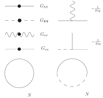
Figure 1: The Feynman rules for the heterotic sigma model. The shaded circles indicate a dressed propagator. The circles indicate that a loop involving only the components of the $\Phi$ superfield receives a factor of $N$. We have suppressed the tensor structure of the rules since only $\delta_{\mu\nu}$ appears.

After a change of variables that renders the kinetic terms canonical, we can continue to negative values of $g$ as in [1] to obtain an $AdS_{D+1}$ heterotic NL$\sigma$M. Quantities that are computed locally and perturbatively, such as $n$-point functions, cannot distinguish between a space of positive or negative curvature. As the beta function is derived from such quantities, it too can be continued to negative $g$, at least order by order in perturbation theory.

The heterotic NL$\sigma$M on $S^{D+1}$ is a generalization of the $O(D+2)$ model, and much of the relevant literature concentrates on an expansion in $1/(D+2)$ rather than $1/D$. We will therefore set

$${N=D+2}$$

(6)

and work with $N$ or $D$, according to convenience, in the rest of this paper.

2.1 Some properties of the heterotic NL$\sigma$M for large $D$

It is known that in the bosonic sigma model a mass appears [9] in the 1/N expansion. The same phenomenon appears in the supersymmetric extension of the sigma model [10, 11] where also the fermions acquire the same mass, signaling chiral symmetry breaking. In the heterotic case the bosons $S$ also acquire the same mass, showing that the interaction term does not destroy this effect. To understand this, let’s start from our action (5), and in the partition function integrate first the fermionic fields and then the bosons, since the action is quadratic in these. We have omitted normalization factors of the partition function in the following.

$${Z}$$

(7)

where the effective action for the Lagrange multiplier fields is given by

$${S_{\rm eff}=\int d^{2}x\left[\frac{1}{4\pi g}\sigma-\frac{N}{4}\mathop{\rm Tr}\nolimits\log(i{\ooalign{\hfil\hfil/\hfil\cr$\partial$}})+\frac{N}{2}\mathop{\rm Tr}\nolimits\log\left(-\partial^{2}-\sigma-\bar{u}\frac{1}{i{\ooalign{\hfil\hfil/\hfil\cr$\partial$}}}u\right)\right]\,.}$$

(8)

Since we are taking the limit $N\rightarrow\infty$ with $g_{0}N$ finite, we see that all terms in the action are of order $N$. We can evaluate this integral by the method of steepest descent, i.e. by finding the classical value of $\sigma$, $u$ that minimizes the exponent, as is done for instance in [12, 13]. This gives the variational equations

$${\langle x|\frac{1}{-\partial^{2}-\sigma(x)-\bar{u}\frac{1}{i{\ooalign{\hfil\hfil/\hfil\cr$\partial$}}}u}|x\rangle}$$

(9)

Because the right hand sides are constant, the left hand sides must also be constant. A solution to these equations is given by

$${u(x)=0\quad\quad\sigma(x)=-m^{2}\,.}$$

(10)

It is easy to see that $\frac{1}{\partial}u(x)=const.$ has as its only solution $u=0$. This is in contrast to the supersymmetric case [12], where there are three solutions. Now $m^{2}$ must satisfy

$${\int d^{2}k\frac{1}{k^{2}+m^{2}}=\frac{1}{2\pi g_{0}}\,.}$$

(11)

Using a simple-momentum cutoff, $\frac{1}{2\pi g_{0}N}=\frac{1}{2\pi}\log\frac{\Lambda}{m}$. By renormalizing at a scale $M$ we get

$${\frac{1}{2\pi g_{0}N}=\frac{1}{2\pi gN}+\frac{1}{2\pi}\log\frac{\Lambda}{M}\,.}$$

(12)

Solving for the mass $m$ we get $m=M\exp[-1/gN]$. Since this is a physical mass we expect that it does not depend on the renormalization scale. Using the Callan-Symanzik equation for $m$,

$${\left(M\frac{\partial}{\partial M}+\beta(g)\frac{\partial}{\partial g}\right)m(g,M)=0\,,}$$

(13)

gives the beta function $\beta(g)=-g^{2}N$. The mass is the same in the bosonic, supersymmetric, [9, 11] and heterotic model. This could have been predicted since the first order $\beta$ function is the same in all models, $\beta_{ij}=\alpha^{\prime}R_{ij}$. Another way to get the same result is to calculate the effective potential for the $\sigma$ field and see that the minimum of the potential is not at zero but at $\sigma=Me^{-1/gN}$. One can go further and examine the effective action (8). It is easy to evaluate the counterterms needed for one-loop renormalization, as we have already computed the wave function renormalization of the $\sigma$ field, and doing so one finds

$${\mathcal{L}_{0,\rm eff}=\frac{1}{4\pi g}\left(1+gN\log\frac{\Lambda^{2}}{M^{2}}\right)\sigma-\frac{N}{4}\mathop{\rm Tr}\nolimits\log{\ooalign{\hfil\hfil/\hfil\cr$\partial$}}+\frac{N}{2}\mathop{\rm Tr}\nolimits\log\left(-\partial^{2}-\sigma-\bar{u}\frac{1}{i{\ooalign{\hfil\hfil/\hfil\cr$\partial$}}}u\right)\,.}$$

(14)

The bare and the dressed quantities are related by

$${\sigma_{0}=Z\sigma\qquad u_{0}=Z^{1/2}u\qquad g_{0}=Z^{-1}g\qquad Z=1+\frac{gN}{2}\log\frac{\Lambda^{2}}{M^{2}}\,.}$$

(15)

Calculating the quadratic terms in the fields $u$, $\sigma$ will give us the propagators for these fields. We can easily find

$${S_{\rm eff}=\frac{N}{2}Tr\frac{1}{-\partial^{2}-m^{2}}\bar{u}\frac{1}{i{\ooalign{\hfil\hfil/\hfil\cr$\partial$}}-m}u-\frac{N}{4}\mathop{\rm Tr}\nolimits\frac{1}{-\partial^{2}-m^{2}}\sigma\frac{1}{-\partial^{2}-m^{2}}\sigma\,.}$$

(16)

The next step is to evaluate the propagators. One finds [11, 12]

$${S_{u}(k)=-\frac{2i}{N}({\ooalign{\hfil\hfil/\hfil\cr$k$}}-2m)V(k^{2})\qquad D_{\sigma}(k)=\frac{2i}{N}(4m^{2}-k^{2})V(k^{2})\,,}$$

(17)

where in $d$ dimensions

$${V(k^{2})=\frac{(4\pi)^{d/2}}{4\Gamma(2-d/2)}\left(\frac{4m^{2}-k^{2}}{4}\right)^{1-d/2}\left({}_{2}F_{1}(2-d/2,1/2,3/2;\frac{k^{2}}{k^{2}-4m^{2}})\right)^{-1}\,.}$$

(18)

In two dimensions this simplifies to

$${V(k^{2})=\pi\sqrt{\frac{k^{2}}{k^{2}-4m^{2}}}\left(\mathop{\rm arctanh}\nolimits\sqrt{\frac{k^{2}}{k^{2}-4m^{2}}}\right)^{-1}\,.}$$

(19)

It is easy to see that the $u$ propagator in $d=2$ dimensions has a pole at $k^{2}=4m^{2}$. This means that there is a particle with this mass. Since the classical equations give $u=-iS{\ooalign{\hfil\hfil/\hfil\cr$\partial$}}\Psi$, there is a boson-fermion bound state, created by the operator $S{\ooalign{\hfil\hfil/\hfil\cr$\partial$}}\Psi$. This is in agreement with [11], but there is no supersymmetric corresponding fermion-fermion bound state, since the Gross-Neveu interaction that is responsible for it is absent.

One can also extend the calculation of [12, 14] to show that there is no multi-particle production in the heterotic sigma model. For example, the process $2\rightarrow 4$ particles can be shown to vanish. The reasoning is that the formalism of [14], valid for the bosonic case, can be extended to include superfields.

3 Critical exponents in the $1/D$ expansion

3.1 General discussion

The method used to determine the critical exponents is the one developed in [8, 15] for the bosonic model and extended to the supersymmetric case in [16, 17]. To this end one writes expressions for the propagators of the fields near the critical point. In keeping with the notation of [8, 15, 18] we assign dimensions to the fields

$${\mathop{\rm dim}\nolimits[S]}$$

(20)

For small but non-zero $x$, the two-point functions may be expanded as follows:

$${G_{SS}(x)}$$   

  

where

$${\gamma_{P}=\rho^{0}\rho^{1}=\left(\begin{array}[]{cc}1&0\\ 0&-1\end{array}\right)}$$

(22)

is the chirality matrix in $2$ dimensions. We have omitted the $O(N)$ indices because both the propagators and the vertex are proportional to $\delta_{\mu\nu}$. So all Green’s functions can be expressed as a scalar function times products of $\delta_{\mu\nu}$, and one does not have to worry about tensor structures of the form $(x-y)^{\mu}(x-y)^{\nu}$. Then one can write the Dyson equations in a $1/D$ expansion for the propagators. Graphical expressions of these equations are shown in figures 2 through 5. The Dyson equations impose consistency conditions on the critical exponents that determine them completely. The graphs that appear in the Dyson equations are the 1PI graphs with the exception of graphs which contain subgraphs that already appear in the Dyson equations at a lower effective loop order: in other words, we exclude diagrams that are already taken into account by expressions for the corrected propagators. The effective loop order is the number of loops minus the number of loops involving only the components of the $\Phi$ superfield.

The left hand side of each Dyson equation is a 1PI propagator, which is the inverse of the connected two-point function. These inverse propagators are computed by first passing to Fourier space using

$${\int d^{d}k\frac{e^{-ik\cdot x}}{k^{2\Delta}}=\frac{\pi^{\mu}\alpha(\Delta)2^{2(\mu-\Delta)}}{x^{2(\mu-\Delta)}}\,.}$$

(23)

The inverse propagators are found to be

$${G_{SS}^{-1}(x)}$$

(24)

where

$${\mu=d/2\qquad\Delta_{S}=\mu-1+\eta/2\qquad\Delta_{\sigma}=2-\eta-\chi\,,}$$

(25)

and for arbitrary $y$,

$${\alpha(y)=\frac{\Gamma(\mu-y)}{\Gamma(y)}\qquad p(y)=\frac{\alpha(y-\mu)}{\pi^{2\mu}\alpha(y)}\qquad r(y)=\frac{yp(y)}{\mu-y}}$$

(26)

To calculate the beta function, one first evaluates the critical exponents of the model at the fixed point in $d=2+\epsilon$ dimensions and then uses the relation

$$\lambda=-\frac{1}{2}\beta^{\prime}(g_{c})\,,$$ (27)

valid at the critical point, to extract $\beta(g)$. This is possible because, in dimensional regularization with minimal subtraction, the only $\epsilon$ dependence in $\beta(g)$ is an overall additive term: see [1] for details. Expanding in $1/D$ with $\kappa=gD$ held fixed, one finds

$$\lambda(\epsilon)=\sum_{i=0}^{\infty}\frac{\lambda_{i}(\epsilon)}{D^{i}}\qquad\frac{\beta(g)}{g}=\epsilon-\kappa+\sum_{i=1}^{\infty}\frac{b_{i}(\kappa)}{D^{i}}$$ (28)

where

$${\lambda_{0}(\kappa_{c})=\frac{\kappa_{c}}{2}\qquad b_{1}(\kappa)=-2\kappa\int_{0}^{\kappa}d\xi\frac{\lambda_{1}(\xi)}{\xi^{2}}\qquad b_{2}(\kappa)=-2\kappa\int_{0}^{\kappa}d\xi\frac{\lambda_{2}(\xi)-b_{1}(\xi)\lambda^{\prime}_{1}(\xi)}{\xi^{2}}\,.}$$

(29)

Note that the critical exponent $\lambda$ is a measurable quantity and as such it should not depend on the renormalization scheme used. Passing from the $\lambda_{i}(\kappa)$ to the $b_{i}(\kappa)$ does introduce significant scheme dependence.

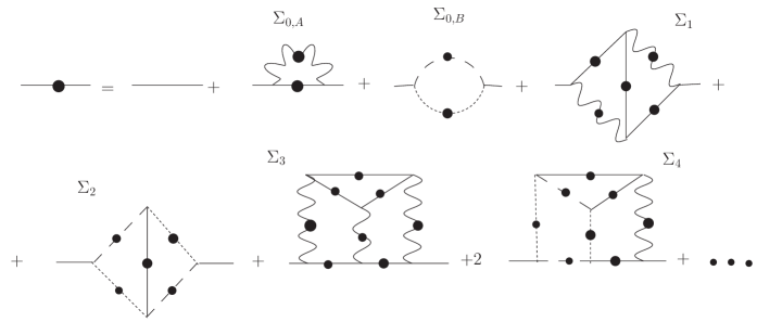
Figure 2: The Dyson equations for the $S$ propagator.

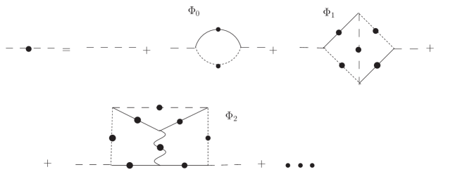
Figure 3: The Dyson equations for the $\Psi$ propagator.

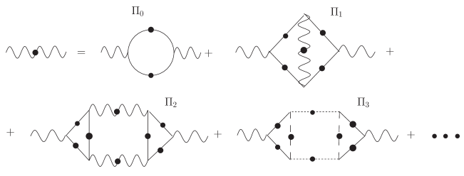
Figure 4: The Dyson equations for the $\sigma$ propator.

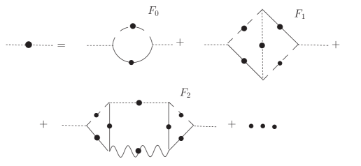
Figure 5: The Dyson equations for the $u$ propagator.

3.2 Critical exponents at order $1/D$

The Dyson equations can be expressed in terms of parameters

$${w=\frac{\Gamma_{SS}^{2}\Gamma_{\sigma\sigma}}{(2\pi g)^{2}}\qquad v=\frac{\Gamma_{SS}\Gamma_{\Psi\Psi}\Gamma_{uu}}{(2\pi g)^{2}}\,,}$$

(30)

which can be regarded as dressed vertex factors for the two vertices shown in figure 1. The leading non-trivial Dyson equations come from the graphs labeled $\Sigma_{0,A}$, $\Sigma_{0,B}$, $\Phi_{0}$, $\Pi_{0}$, and $F_{0}$ in figures 2 through 5: the tree-level graphs make no contribution to the leading scaling behavior. The quantities $\Gamma^{\prime}_{SS}$, $\Gamma^{\prime}_{\Psi\Psi}$, $\Gamma^{\prime}_{\sigma\sigma}$, and $\Gamma^{\prime}_{uu}$ describe how far one is removed from the fixed point; so in particular one must be able to set them all to zero and get a self-consistent set of equations. Then the dependence of each graph on the position-space separation $x$ is just an overall power of $x$. Matching these overall powers leads simply to the constraint $\chi=0$. Matching other factors leads to the equations

$${p(\Delta_{S})+w+v}$$   

  

which determine the quantities $\Delta_{S}$, $\Delta_{\sigma}$, $w$, and $v$ as functions of $\mu$ and $N$. The system is in fact over-determined if we recall the relations (25) and the constraint $\chi=0$. But we will see in section 4.1 that $\chi=0$ is only a leading order result; thus to solve (31) we expand

$${\eta=\sum_{i\geq 0}\frac{\eta_{i}}{D^{i}}\qquad\chi=\sum_{i\geq 0}\frac{\chi_{i}}{D^{i}}\qquad w=\sum_{i\geq 0}\frac{w_{i}}{D^{i}}\qquad v=\sum_{i\geq 0}\frac{v_{i}}{D^{i}}\,.}$$

(32)

Then one straightforwardly extracts from (31) the coefficients

$${\eta_{0}}$$

(33)

Higher order coefficients receive contributions from higher order graphs. Note that $\chi_{0}=0$ could be obtained either from matching overall powers of $x$ or from the equations (31).

Now consider non-zero coefficients $\Gamma^{\prime}_{SS}$, $\Gamma^{\prime}_{\Psi\Psi}$, $\Gamma^{\prime}_{\sigma\sigma}$, and $\Gamma^{\prime}_{uu}$: this corresponds to moving away from the fixed point. Linearizing the Dyson equations leads to the constraints

$${-p(\Delta_{S})q(\Delta_{S},\lambda)\Gamma^{\prime}_{SS}+w(\Gamma^{\prime}_{SS}+\Gamma^{\prime}_{\sigma\sigma})+v(\Gamma^{\prime}_{\Psi\Psi}+\Gamma^{\prime}_{uu})}$$

(34)

Graphically, these equations arise from using the leading power-law expressions (e.g. $\Gamma_{SS}/x^{2\Delta_{S}}$ rather than $G_{SS}(x)$) for all propagators except one, chosen arbitrarily; and for that one, use the correction term (e.g. $\Gamma_{SS}\Gamma^{\prime}_{SS}/x^{2\Delta_{S}-2\lambda}$). The linear equations (34) must admit a non-zero solution for $\Gamma_{SS}^{\prime}$, $\Gamma_{\Psi\Psi}^{\prime}$, $\Gamma_{\sigma\sigma}^{\prime}$, $\Gamma_{uu}^{\prime}$ in order for the correction terms to describe a genuine deformation of the critical point. So the corresponding determinant must vanish, which leads to

$${{}\left[(w+v)q(\Delta_{S},\lambda)+w\left(1-\frac{2}{q(\Delta_{\sigma},\lambda)}\right)-\frac{v}{s(\Delta_{\sigma}-1,\lambda)}\right](1-s(\Delta_{\sigma},\lambda)s(\Delta_{\sigma}-1,\lambda))}$$

(35)

Note that setting $v=0$ gives the equation valid for the bosonic model as expected. To simplify (35), one can use (33) and note that $w_{1}=v_{1}\frac{2-\mu}{\mu-1}$. So far we have not used any expansion in $1/D$. Using the expansions (32) and

$${\lambda=\sum_{i\geq 0}\frac{\lambda_{i}}{D^{i}}}$$

(36)

we can determine

$${\lambda_{0}=\mu-1\qquad\lambda_{1}=\frac{1}{2}(2\mu-1)(\mu-1)\eta_{1}\,.}$$

(37)

Another way to compute the original determinant, is the following: one notes that $r(\Delta_{S})s(\Delta_{S},\lambda)\sim 1/D^{0}$, while all other terms scale at least as $1/D^{1}$. This means that, in expanding the $4\times 4$ determinant of (34), the first order contribution comes only from the determinant of the $3\times 3$ matrix

$${AI\equiv\left(\begin{array}[]{ccc}-p(\Delta_{S})q(\Delta_{S},\lambda)+w&w&v\\ w&-p(\Delta_{\sigma})q(\Delta_{\sigma},\lambda)/N&0\\ v&0&-r(\Delta_{\sigma}-1)s(\Delta_{\sigma}-1,\lambda)/N\end{array}\right)\,.}$$

(38)

where in each element of the matrix we only keep the first term in the $1/D$ expansion. This determinant provides the first $1/D$ term of (35) and thus reproduces (37).

It is interesting to compare with the bosonic case. It is easily seen that $\lambda_{1}^{\rm het}={1\over 2}\lambda_{1}^{\rm bos}$, even though $\eta^{\rm het}_{1}$, $w_{1}$, and $v_{1}$ are not so simply related to $\eta^{\rm bos}_{1}$ and the corresponding vertex factor for the bosonic case. The relation $\lambda_{1}^{\rm het}={1\over 2}\lambda_{1}^{\rm bos}$ is expected: we know that $\lambda_{1}^{\rm sup}=0$ in the type II case, and having half the fermions in the heterotic case will cancel only half the bosonic contribution.

3.3 A check of the calculation

Following [18], we see that $\eta$ is the anomalous dimension of the $S$ propagator. So far we have computed it in the $1/D$ expansion using techniques in position space. One can also straightforwardly compute $\eta_{1}$ in momentum space using the expressions for the propagators that we have previously found (17). Firstly we note that for small $k$,

$${\tilde{G}_{SS}(k)\sim k^{-2+\eta}\sim k^{-2+\eta_{o}}\left(1+\frac{\eta_{1}}{N}\log k+\mathcal{O}(1/N^{2})\right)\,,}$$

(39)

with $\tilde{G}_{SS}$ the Fourier transform of the $S$ propagator. But $\tilde{G}_{SS}(k)$ can also be determined from the one-particle irreducible diagrams $\Sigma(k^{2})$:

$${\tilde{G}_{SS}^{-1}(k)=k^{2}+\Sigma(k^{2})-\Sigma(0)\sim k^{2}(1-\frac{\eta_{1}}{N}\log k)\,,}$$

(40)

since $\eta_{0}=0$. Having calculated the propagators of the lagrange multiplier fields it is straightforward to compute the $\Sigma(k^{2})$ from the one-loop diagrams. We find

$${\Sigma(k^{2})}$$

(41)

where we have put $m^{2}=0$ as usual [17], and $M$ is the cutoff. One notes that, for small $k$ the $k^{2}\log k$ behavior comes from the small $p$ region [18]. The integral is trivial to do, and for the $k^{2}\log k$ part it gives

$${\Sigma(k^{2})=-\frac{2^{d-1}}{Nd}\frac{1}{{}_{2}F_{1}(2-d/2,1/2,3/2,1)\Gamma(2-\frac{d}{2})\Gamma(\frac{d}{2})}k^{2}\log k\,.}$$

(42)

It is easy to see using $d=2\mu$ and properties of the Gamma function that this coincides with the expression for $\eta_{1}$ in (33). An easier way to do the checking is the following. One can write similar expressions for $\Sigma(k^{2})$ for the bosonic and supersymmetric models [8, 17]. Then it is easy to observe that

$${\Sigma_{\rm bos}(k^{2})-\Sigma_{\rm bos}(0)=-\Sigma_{\rm sup}(k^{2})+2\Sigma_{\rm het}(k^{2})\,.}$$

(43)

This easily gives

$${2\eta_{\rm het}=\eta_{\rm bos}+\eta_{\rm sup}\,.}$$

(44)

With [8, 17]

$${\eta_{\rm bos}=\frac{(2-\mu)}{\mu}\eta_{\rm sup}\qquad\eta_{\rm sup}=\frac{4}{N}\frac{\Gamma(2\mu-2)}{\Gamma^{2}(\mu-1)\Gamma(2-\mu)\Gamma(\mu)}}$$

(45)

we find $\eta_{\rm het}=\frac{1}{\mu}\eta_{\rm sup}$ which agrees with (33).

4 Results at order $1/D^{2}$

Each graph in figures 2-5 carries an overall factor $1/D^{M}$ where $M$ is the number loops minus the number of loops containing only $S$ and $\Psi$. To see this, first note that each propagator $G_{XX}$ carries a factor $\Gamma_{XX}$ (where $X=S$, $\Psi$, $\sigma$, or $u$). Next note that the amplitude for each graph must contain an overall factor which is a product of the factors $w=\Gamma_{SS}^{2}\Gamma_{\sigma\sigma}/(2\pi g)^{2}$ and $v=\Gamma_{SS}\Gamma_{\Psi\Psi}\Gamma_{uu}/(2\pi g)^{2}$, one for each vertex in the graph. The overall factor $1/D^{M}$ arises because $w$ and $v$ scale as $1/D$ and because each loop containing only $S$ and $\Psi$ carries a factor of $N$. The graphs in figures 2 and 3 are those with $M\leq 2$, and the ones in figures 4 and 5 are those with $M\leq 1$. Together, these are all the graphs that can contribute to $\eta$, $w$, $v$, and $\lambda$ through order $1/D^{2}$, and they also determine $\chi$ through order $1/D$. Because we quote final results in terms of $1/D$, we must keep in mind the relation between expansions in $1/N$ and $1/D$:

$${w=\sum_{i\geq 0}{\tilde{w}_{i}\over N^{i}}=\sum_{i\geq 0}{w_{i}\over D^{i}}\qquad w_{1}=\tilde{w}_{1}\quad w_{2}=\tilde{w}_{2}-2\tilde{w}_{1}\,,}$$

(46)

with similar relations for other quantities.

4.1 Calculation of $\eta_{2}$

A technical complication arises in the $1/D^{2}$ corrections to the Dyson equations that was explained and resolved in [8, 15]. The problem is that the higher-loop graphs diverge when $\chi=0$. In fact, $\chi=0$ only up to $1/D$ corrections. But it convenient to regularize the “divergence” and extract finite expressions for the two-loop Dyson equations through the following steps:

1. Shift $\chi\to\chi+\Delta$.

2. Expand the amplitudes for individual graphs in powers of $\Delta$.

3. Cancel $1/\Delta$ terms against certain counter-terms in the lagrangian.

4. Fix $\chi_{1}$ by setting to zero certain terms in the Dyson equation which depend logarithmically on the position-space separation $x$ and which, if non-zero, would spoil self-consistency.

We will now go through these steps in detail for the $\Psi$ propagator. The reader who wishes to bypass the technical details can skip to (56) and (57), which are the two-loop Dyson equations with all divergences removed. But the results (54) and (58) for $\chi_{1}$ provide important consistency checks.

When $\chi\neq 0$, $x$ dependence cannot be canceled out of the Dyson equations in a simple way: setting $\Gamma^{\prime}_{SS}=\Gamma^{\prime}_{\Psi\Psi}=\Gamma^{\prime}_{\sigma\sigma}=\Gamma^{\prime}_{uu}=0$, one obtains for the $\Psi$ propagator’s Dyson equation

$${r(\Delta_{S})+v(x^{2})^{\chi}+v^{2}(x^{2})^{2\chi}\Phi_{1}+Nwv^{2}(x^{2})^{3\chi}\Phi_{2}=0\,.}$$

(47)

Here $\Phi_{1}$ and $\Phi_{2}$ are functions of $\Delta_{S}$, $\Delta_{\sigma}$, and $\mu$ which diverge when $2\Delta_{S}+\Delta_{\sigma}-2\mu=-\chi=0$. Although these are in some sense an artifact of a limit ($\chi\to 0$) which one cannot take independently of the large $N$ limit, it is convenient nevertheless to regulate them, as explained above, by shifting

$${\chi\to\chi+\Delta\,.}$$

(48)

The amplitudes $\Phi_{1,2}$ may then be expanded as

$${\Phi_{i}={X_{i}\over\Delta}+\Phi_{i}^{\prime}+O(\Delta)\,,}$$

(49)

where both $X_{i}$ and $\Phi_{i}^{\prime}$ are functions of $\Delta_{S}$, $\Delta_{\sigma}$, and $\mu$, subject to $2\Delta_{S}+\Delta_{\sigma}-2\mu=0$. In appendix C we exhibit $\Phi_{1,2}$ in the form (49), as well as a number of related quantities that enter into other Dyson equations. To cancel the divergent $1/\Delta$ terms in $\Phi_{1,2}$, one may rescale the lagrange multiplier fields in the original action (3). This rescaling amounts to adding counter-terms to the action, and it can be expressed, to the relevant order, as

$${v\to\left(1+{m_{1}\over N}\right)v\qquad w\to\left(1+{m_{1}\over N}\right)w\,.}$$

(50)

(The factor on $v$ and $w$ is the same because of supersymmetry.) Subjecting (47) to the shift (48) and the rescaling (50), it becomes, keeping terms up to $1/N^{2}$,

$${{}r(\Delta_{S})+(x^{2})^{\chi}\Big{(}v+v^{2}\Phi^{\prime}_{1}+Nv^{2}w\Phi^{\prime}_{2}\Big{)}+}$$

(51)

The last line contains all the divergent pieces. Setting $\chi=0$ [8] and taking the limit $\Delta\to 0$ determines $m_{1}$ as

$${-v_{1}\frac{m_{1}}{N}=v_{1}^{2}\frac{X_{1}}{\Delta}+Nv_{1}^{2}w_{1}\frac{X_{2}}{\Delta}\,.}$$

(52)

Plugging (52) back into (51), and now considering a finite $\chi$ we get

$${r(\Delta_{S})+(x^{2})^{\chi}\left(v+v^{2}\Phi^{\prime}_{1}+Nv^{2}w\Phi^{\prime}_{2}\right)+v_{1}^{2}X_{1}\left(\frac{(x^{2})^{2\chi}-(x^{2})^{\chi}}{\chi}\right)}$$

(53)

When one expands $\chi=\chi_{1}/N+O(N^{-2})$, there are terms that behave as $\log x^{2}$. One gets rid of these if $\chi_{1}$ obeys

$${\chi_{1}=-v_{1}X_{1}-2v_{1}w_{1}X_{2}\,.}$$

(54)

We could have derived (52),(54) purely within the $N\to\infty$ limit. In this setup there is no need for $\Delta$ and $\chi$ is taken to be finite. Note that it behaves as $\chi\sim 1/N$ since $\chi_{0}=0$ (33). The Dyson equation after the rescaling (50) is (51) with $\Delta$ replaced with $\chi$. In taking the $N\to\infty$ limit there are terms that diverge linearly with $N$ and terms that behave as $\log x^{2}$. Respectively these are

$${(x^{2})^{\chi}\big{(}v_{1}\frac{m_{1}}{N}+v_{1}^{2}\frac{X_{1}}{\chi}+Nv_{1}^{2}w_{1}\frac{X_{2}}{\chi}\big{)}}$$

(55)

Setting these to zero fixes $m_{1},\chi_{1}$ as in (52),(54), with $\Delta$ replaced by $\chi$. We choose to keep the $\Delta$ shift, as is common in the literature [8, 15, 19, 20]. If one wishes to translate our results, in the $N\to\infty$ formalism, only a simple substitution of $\Delta\to\chi_{1}/N$ is needed in the values of the diagrams given in Appendix C. What is left is the finite correction to the leading Dyson equation for the $\Psi$ propagator:

$${r(\Delta_{S})+v+v^{2}\Phi^{\prime}_{1}+Nwv^{2}\Phi^{\prime}_{2}=0\,.}$$

(56)

Following the same procedure for the $S$, $\sigma$, and $u$ Dyson equations, one gets the finite equations

$${p(\Delta_{S})+w+v+w^{2}\Sigma^{\prime}_{1}-v^{2}\Sigma^{\prime}_{2}+Nw^{3}\Sigma^{\prime}_{3}-2Nv^{2}w\Sigma^{\prime}_{4}}$$

(57)

where $\Sigma^{\prime}_{i}$, $\Pi^{\prime}_{i}$, and $F^{\prime}_{i}$ are the finite parts of $\Sigma_{i}$, $\Pi_{i}$, and $F_{i}$, listed in Appendix C. The minus signs in (57) come from fermion loops. From each Dyson equation one also gets a new determination of $m_{1}$ and $\chi_{1}$:

$${m_{1}}$$   

  

  

where $P_{i}$, $S_{i}$, $Y_{i}$ are the residues of $\Pi_{i}$, $\Sigma_{i}$, and $F_{i}$, respectively.

Fortunately, the four seemingly independent determinations of $m_{1}$ and $\chi_{1}$ all agree, as one can check by explicitly evaluating (52), (54), and (58) using expressions from Appendix C with $\Delta_{S}=\mu-1$ and $\Delta_{\sigma}=2$. This provides a check that the renormalization procedure we have chosen to cancel the divergences of higher-loop graphs is consistent. Other schemes change the values for individual amplitudes, but the critical exponents remain the same [16].

Interestingly, there is yet another consistency check on $\chi_{1}$. One can show from (54) or (58) that

$${\chi_{1}=\mu(2\mu-3)\eta_{1}\,.}$$

(59)

This is seen to comply with a scaling law formulated for the bosonic model in [18]:

$${2\lambda=2\mu-\Delta_{\sigma}\,.}$$

(60)

That this relation is also valid in our case can be seen by applying the Callan-Symanzik equation near the critical point for $\langle\sigma(p)\sigma(-p)\rangle$ or $\langle\bar{u}(p)u(-p)\rangle$ propagator.

Now we can solve (56)-(57) by eliminating $w$ and $v$:

$${r(\Delta_{S})=\frac{1}{N}r(\Delta_{\sigma}-1)+\frac{v_{1}^{2}}{N^{2}}(F_{1}^{\prime}-\Phi_{1}^{\prime})+\frac{w_{1}v_{1}^{2}}{N^{2}}(F_{2}^{\prime}-\Phi_{2}^{\prime})\,.}$$

(61)

Expanding $\Delta_{S},\Delta_{\sigma}$ in (61), we can determine $\tilde{\eta_{2}}$

$${\frac{\tilde{\eta}_{2}}{\eta_{1}^{2}}}$$

(62)

where $H(x)=\psi(x+1)-\psi(1)$ and the $B(x)$ function is defined in the appendix. The first line just comes from the Hatree-Fock diagrams, i.e. by iterating the 1/N Dyson equation to the next order, the second is the contribution of $\Phi_{1},F_{1}$ and the third comes from $\Phi_{2},F_{2}$. We also can determine the values of $w_{2},v_{2}$ as

$${\frac{\tilde{w}_{2}}{\eta_{1}w_{1}}}$$

(63)

$${\frac{\tilde{v}_{2}}{\eta_{1}v_{1}}=\frac{\tilde{\eta_{2}}}{\eta_{1}^{2}}-\frac{1}{2\mu}-\frac{\mu}{2}+\mu(\mu-2)+2\mu(\mu-2)\left(B(2)-B(\mu-1)\right)\,.}$$

(64)

In (63), the first three terms come from iteration of the first order equations, while in (64), the first two terms come from such iteration.

4.2 Calculation of $\lambda_{2}$

As in section 3.2, the calculation of $\lambda_{2}$ through order $1/D^{2}$ requires evaluating each graph with one propagator altered from its leading power behavior (e.g. $\Gamma_{SS}/x^{2\Delta_{S}}$ for an $S$ propagator) to its sub-leading power behavior (e.g. $\Gamma_{SS}\Gamma^{\prime}_{SS}/x^{2\Delta_{S}-2\lambda}$). The four Dyson equations lead to four linear equations in the quantities $\Gamma^{\prime}_{SS}$, $\Gamma^{\prime}_{\Psi\Psi}$, $\Gamma^{\prime}_{\sigma\sigma}$, and $\Gamma^{\prime}_{uu}$:

$${(-p(\Delta_{S})q(\Delta_{S},\lambda)+w+\Sigma_{S})\Gamma_{SS}^{\prime}+(w+\Sigma_{\sigma})\Gamma_{\sigma\sigma}^{\prime}+(v+\Sigma_{u})\Gamma_{uu}^{\prime}+(v+\Sigma_{\Psi})\Gamma_{\Psi\Psi}^{\prime}}$$

(65)

where for example we denote by $\Sigma_{\Psi}$ all the diagrams that appear in the $S$ propagator where the $\Psi$ propagator is corrected. As in section 4.1, the amplitudes diverge when $2\Delta_{S}+\Delta_{\sigma}-2\mu\to 0$, and the same procedure described there to regulate and subtract the divergences and to remove terms proportional to $\log x^{2}$ carries over to the present case. The finite parts of all the quantities in (65) are given in Appendix D, as well as some further remarks on their evaluation.

The system (65) must have a nonzero solution for the $\Gamma$’s, so the determinant must be zero. This determines $\lambda_{2}$. A way to calculate the determinant to sufficient accuracy is to note that $r(\Delta_{S})s(\Delta_{S},\lambda)\sim 1/N^{0}$, and then expand the determinant into three $3\times 3$ determinants, i.e. expanding in the line of $\Psi$ field Dyson equation. All terms have to be expanded up to $1/N^{2}$ accuracy. One also notes that $\lambda_{2}$ only appears in the expansion of $p(\Delta_{S})q(\Delta_{S},\lambda)$ at this order. So $\lambda_{2}$ is going to be a linear combination of the various sums of diagrams given in the appendix, factors of $w_{2}$ and $v_{2}$, and terms that come from iterating the $1/N$ equations. The final result is quite involved and we prefer to give it implicitly as

$${{\tilde{\lambda}_{2}\over\eta_{1}^{2}}}$$

(66)

The right hand side is a function of $\mu$ which can be obtained explicitly by substituting the expressions (33), (63), (64), (127), (129), (130), (133), (134), and (135) into (66).

4.3 Calculation of the beta function

As explained in section 3.1, we can calculate the beta function once we know $\lambda$. Noting that (66) gives the $1/N^{2}$ expansion term and subtracting $2\lambda_{1}$ we find

$${\lambda_{0}=\epsilon/2,\quad\lambda_{1}(\epsilon)=\frac{\epsilon^{2}}{4}+\frac{\epsilon^{3}}{8}-\frac{\epsilon^{4}}{16}+\mathcal{O}(\epsilon^{5})}$$

(67)

$${\lambda_{2}=\left(\frac{5}{16}+\frac{9}{4}\zeta(3)\right)\epsilon^{4}+\mathcal{O}(\epsilon^{5})\,.}$$

(68)

Using (29), we compute the beta function for the heterotic string in a constant curvature background:

$${\beta(g)=-Dg^{2}-\frac{1}{2}Dg^{3}-\frac{g^{4}D}{4}\left(1+\frac{D}{2}\right)-\frac{g^{5}D^{2}}{4}\left(\frac{3}{2}-\frac{D}{3}\right)-\frac{3}{2}\zeta(3)g^{5}D^{2}+\mathcal{O}(\frac{1}{D^{3}})\,.}$$

(69)

It is obvious that there is agreement with the first two loops of the expression (1), where we use

$${\beta(g)=M\frac{\partial g}{\partial M}=-\frac{g}{N-1}g^{ij}\beta_{ij}}$$

(70)

and (2). We do not know of any calculation of the beta function of the heterotic string in the minimal subtraction scheme that goes beyond two loops. In [21, 22] the beta function was computed using the background field method, and found to be in three loops

$${\beta_{ij}^{(3)}=\frac{\alpha^{\prime 3}}{8}\left(\frac{3}{2}R_{ikjl}R^{kmnp}R^{l}{}_{mnp}-\frac{1}{2}R_{lm}R_{i}{}^{lnp}R_{j}{}^{m}{}_{np}-\frac{1}{2}R_{jl}R^{lmnp}R_{imnp}\right)\,.}$$

(71)

The appearance of the Ricci tensor means that it is not minimal subtraction. Divergences involving the Ricci tensor can only appear through closed loops where at least one propagator starts and ends at the same vertex. Within the minimal subtraction scheme, at more than one loop these terms combined with their counterterms never produce a simple pole [23, 24]. A small check of our result comes from the famous $\zeta(3)$ term, $\frac{\zeta(3)\alpha^{\prime 4}}{2}R_{mhki}R_{jrt}{}^{m}(R^{k}{}_{qs}{}^{r}R^{tqsh}+R^{k}{}_{qs}{}^{t}R^{hrsq})$. This term is identical in the bosonic [25, 26, 27], supersymmetric [23, 24], and heterotic [28] cases. In an expansion of the Virasoro amplitude, it is associated with the constant term in an expansion in the Mandelstam variables $s$, $t$, and $u$. At loop order $n+1$ in NL$\sigma$M calculations, it seems likely that the coefficient of $\zeta(n)$ is the same for the bosonic, supersymmetric, and heterotic cases (see [16] for a comparison of the bosonic and supersymmetric cases).

In [29, 28, 30], the absence of a three-loop term of the form $\alpha^{\prime 3}R^{3}$ was noted. The three-point scattering amplitudes suggest that there are also no $RF^{2}$ or $F^{3}$ in the effective action. One knows that identifying the gauge connection with the spin connection in the heterotic string effective action will give the superstring effective action, where there is no $\alpha^{\prime 3}$ term. So if there were any $R^{3}$ terms in the heterotic case it would not be possible to cancel them. All this seems in conflict with the (69), where the term proportional to $g^{4}$ would seem to correspond to an $R^{3}$ term in the effective action. But it should be noted that the relation between the effective action and the beta function is [31]

$${2\kappa_{D}^{2}\alpha^{\prime}\frac{\delta S_{\rm eff}}{\delta g_{ij}}=K_{ij}^{kl}\beta_{kl}\,,}$$

(72)

where $K_{ij}^{kl}$ can be computed perturbatively. In the bosonic case, this was done in the minimal subtraction scheme in [31, 32]; in the heterotic case, this was done in a different scheme in [21, 22]; but we do not know of a minimal subtraction calculation of $K_{ij}^{kl}$ in the heterotic case. In the bosonic case, $K_{ij}^{kl}$ receives contributions starting at two loops, and it can be shown that this is compatible with an independent calculation of the effective action using scattering amplitudes. The same thing may happen in the heterotic case: in particular, $R^{3}$ terms could indeed be absent from $S_{\rm eff}$, and the $g^{4}$ term in (69) could come entirely from $K_{ij}^{kl}$. A similar conclusion is reached in [33, 34] where it is shown that the beta function of the heterotic string in the presence of background gauge fields has a term at three loops that behaves as $F^{3}$, even though no corresponding term is present in the the effective action.

Finally, it is possible to make a statement about the three-loop structure of the beta function in the $\alpha^{\prime}$ expansion. Excluding the Ricci tensor and the Ricci scalar, since the beta function is computed within the minimal subtraction scheme, the terms that are third order in the Riemann tensor and are compatible with the $g^{4}$ terms in (69) are given by

$${\alpha^{\prime 3}\left(\frac{1}{8}R_{klmn}R_{i}{}^{mlr}R_{j}{}^{k}{}_{lr}-\frac{1}{16}R_{iklj}R^{kmnr}R^{l}{}_{mnr}\right)\,.}$$

(73)

4.4 Singularities of the critical exponents; central charge of the CFT

Because $\lambda$ involves products of $\Gamma$ functions it is natural to investigate the location of its singularities closest to the origin, as in [1]. Because $\lambda_{1}^{het}=\frac{1}{2}\lambda_{1}^{bos}$, the location of the pole of $\lambda_{1}$ coincides with the pole in the bosonic case, with half the residue. One also has to note that $\eta_{1}(\mu)$ behaves as $\eta_{1}\sim-\frac{4}{\pi^{2}}\frac{1}{2\mu-1}$ i.e. it has a simple pole at $\epsilon=-1$. But $\lambda_{1}$’s first singularity is at $\epsilon=-3$, since the pole of $\eta_{1}$ is canceled by a similar pole of $\chi_{1}$. Examining term by term the structure of $\lambda_{2}$ it is easy to see that the singularities of $\lambda_{2}$ come from the $\eta_{1}^{2}$ factor that multiplies the whole expression (66) and from the three-loop diagrams that have the lagrange multiplier field propagator corrected, i.e. $\Pi_{2\sigma}$, $\Pi_{3u}$, $F_{2u}$, and $F_{2\sigma}$. Since

$${R_{3}(\mu)\sim\frac{-1}{2\mu-1},\qquad R_{2}(\mu)\sim\frac{1}{(2\mu-1)^{2}}}$$

(74)

and $\lambda_{2}$ has terms that behave as $\sim R_{3}^{2}\eta_{1}^{2}$ and $R_{2}\eta_{1}^{2}$ times a $\mu$ polynomial with no zero at $\mu=1/2$, we see that it has a fourth order pole. In all, one finds

$${\lambda_{1}=-\frac{3/(4\pi^{2})}{\epsilon+3}+\mathcal{O}(1)\quad\quad b_{1}\ =-\frac{\log(3+\kappa)}{2\pi^{2}}+\mathcal{O}(1)}$$

(75)

$${\lambda_{2}=\frac{8/\pi^{4}}{(\epsilon+1)^{4}}+\mathcal{O}((\epsilon+1)^{-3})\quad\quad b_{2}\ =-\frac{16/3\pi^{4}}{(\kappa+1)^{3}}+\mathcal{O}((\kappa+1)^{-2})\,.}$$

(76)

The $1/(\kappa+1)^{2}$ term in $b_{2}$ comes only from the factors $R_{3}\eta_{1}^{2}$ and from the Hartree-Fock diagrams. The singularities in the heterotic case are at the same locations and of the same order as in the bosonic case.

Because of the sign of $b_{2}$, there is clearly a zero of $\beta(g)$ (computed through order $1/D^{2}$) for negative $g$, close to $\kappa=-1$. The same caveats discussed in [1] apply: higher order terms in $1/D$ could conceivably cause this zero to disappear or move significantly. In section 5 we will comment further on higher-order corrections. For the remainder of this section we will assume that the computation of $\beta(g)$ that we have carried out is precise enough to describe the zero correctly.

The zero of $\beta(g)$ arises through competition between the one-loop term (corresponding to Einstein gravity) and $b_{2}$ (corresponding to a combination of all $\alpha^{\prime}$ corrections to Einstein gravity). Because the geometry has string scale curvatures (more precisely, $L^{2}\sim D\alpha^{\prime}$) there is no reason to think that the worldsheet central charges are particularly close to the flat-space results. Fortunately, one can calculate the central charges using Zamolodchikov’s c-theorem:

$${\frac{\partial c}{\partial g}=\frac{3(D+1)}{2g^{2}}\beta(g)\,.}$$

(77)

The result (77) holds for both the holomorphic and the anti-holomorphic sides: $c$ and $\tilde{c}$ differ by a constant. To derive the prefactor on the right hand side of (77), one can consider two-point functions of the graviton perturbation $O_{ij}=\frac{1}{2\pi\alpha^{\prime}}\partial X_{i}\bar{\partial}X_{j}+\frac{1}{4\pi}\Psi\partial\Psi$ around flat space, as is done in [1]. This prefactor receives higher loop corrections, and knowing $K^{kl}_{ij}$ in higher loops, one can in principal compute them. As in the bosonic and supersymmetric cases, the results suggest that with increasing $D$ the critical point moves closer to $\kappa=-1$: integrating (77) leads to

$${c}$$

(79)

where we have noted that the central charge of the holomorphic side in flat space is $c=D+1$, while for the anti-holomorphic side it is $\tilde{c}=\frac{3}{2}(D+1)$. The approximate equalities arise from dropping the $b_{1}(\kappa)$ and $b_{2}(\kappa)$ terms from the integrand: their only role at this level of approximation is to set $\kappa_{c}$. As $\kappa_{c}$ gets closer to $-1$ (i.e. as $D$ becomes large), the central charges converge to

$${c=\frac{5}{2}(D+1)\qquad\tilde{c}=3(D+1)\,.}$$

(80)

The result (80) for $c$ is the same as in the bosonic case, while for $\tilde{c}$ it is the same as the type II case [1]. As in [1], (80) appears to set only an approximate upper bound on the central charges. The dominant error in the calculation 79 is from the uncertainty in the prefactor in (77). Analogous to the speculations in [1], it is conceivable that the expressions (80) might in fact be exact. But this would require a significant conspiracy between the prefactor in (77) and the beta function.

The fact that the location of the critical point at finite $D$ is so close to the singularity of $\lambda$ means that the critical exponent $\lambda$ evaluated at the critical point is large and positive. This leads to an operator with a large and negative dimension, which appears to violate unitarity. However, one could hope that a consistent GSO projection would project this operator out of the spectrum.

5 Discussion

The existence of the $AdS_{D+1}$ critical point depends on competition between one-loop and $1/D^{2}$ effects. It would therefore be instructive to compute the beta function through order $1/D^{3}$ and see whether the fixed point persists. Given that the number of diagrams needed for the computation at the next order grows significantly, the shortest path seems to be calculating $\chi_{3}$ and using (60) to deduce $\lambda_{3}$. However, note that for the calculation of $\chi_{3}$ one needs to derive the residues of diagrams at order $1/D^{4}$, which include some six-loop diagrams.

There is some reason to think that the singularities of $\lambda$ at order $1/D^{3}$ are no worse than at order $1/D^{2}$: examining the diagrams needed for the Dyson equations of the Lagrange multiplier fields, we see that at order $1/D^{3}$ these come from either inserting a $\sigma$ or $u$ propagator in the $1/D^{2}$ diagrams or inserting a loop of $S$ or $\Psi$ in the middle of the diagram. The computation for the diagrams that come from inserting a $\sigma$ or $u$ propagator can easily be seen to be reduced to the sum of diagrams similar to $\Pi_{2}$ or $\Pi_{3}$ with one different exponent. A naive calculation does not produce any worse singularities than the ones already contained in $\Pi_{2}$ and $\Pi_{3}$. However, one also has to compute the more difficult diagrams with the additional $S$ or $\Psi$ loop.

It is evident that the methods of [8, 15], has many advantages over calculating Feynman diagrams in momentum space. In the latter approach one encounters difficulties already in calculating second order diagrams, since the propagators of the Lagrange multiplier fields are in general hypergeometric functions. It is noteworthy that even though we start from $d=2+\epsilon$ dimensions, one can calculate critical exponents of the $O(N)$ model in any dimension $2<d<4$, and there is agreement with the results in three dimensions [38] in the bosonic case.

Perhaps the methods of [8, 15] could be applied to a related quantum field theory:

$${S=\int d^{d}x\,\left(\frac{1}{2}\nabla\vec{\Phi}\cdot\nabla\vec{\Phi}+\frac{1}{2}\lambda\sigma\vec{\Phi}\cdot\vec{\Phi}-\frac{\lambda N}{4}\sigma^{2}\right)\,,}$$

(81)

which for $d=3$ is the proposed dual of an $AdS_{4}$ vacuum of a theory with arbitrarily high spin gauge fields [39]. What makes (81) susceptible to a position-space treatment analogous to those in [8, 15] is that only cubic vertices are involved. It would be interesting to compute, for example, the four point function of $\sigma$ to order $1/N^{2}$ and compare it to the corresponding $AdS_{4}$ calculation, as is done for example in [40] at order $1/N$.

Appendix A Anomalies

Since we have coupled only the right moving fermions to gravity it is natural to investigate whether there are anomalies. These are related to a breakdown of general coordinate invariance or local Lorentz invariance. We will investigate only the latter, as is usually done [41]. Indeed when there is a coordinate anomaly one can add a counterterm to the action and convert it to a Lorentz anomaly [42]. It is convenient to use the tetrad formalism. Local Lorentz transformations in this formalism are given by

$${e^{\prime}_{\mu}{}^{p}(x)=e_{\mu}{}^{q}(x)\Theta^{p}{}_{q}(x)\,.}$$

(82)

The Riemann tensor can be written $R_{\mu\nu}{}^{p}{}_{q}$, with mixed spacetime and tangent space indices, and can be regarded as a two form $R_{2}$. We only have to worry about the massless fields of the supergravity sector [41]. The anomaly polynomials for the spinor and the gravitino contain only terms that are proportional to polynomials in $\mathop{\rm Tr}\nolimits R_{2}^{\wedge 2m}$. In the AdS space that we are interested in we can calculate

$${R_{\mu\nu}{}^{a}{}_{b}R_{\kappa\lambda}{}^{c}{}_{a}=\frac{1}{L^{2}}(\delta^{c}{}_{k}R_{\mu\nu\lambda b}+\delta^{c}{}_{\lambda}R_{\mu\nu b\kappa})}$$

(83)

which when antisymmetrizing to get the wedge product returns zero. So $R_{2}\wedge R_{2}=0$ in our case, and we do not have to worry about the gravitational anomalies. Another way to view this is to say that the field strength $H_{3}=dB_{2}$ obeys the modified Bianchi identity

$${dH_{3}=\frac{1}{4\pi}(\mathop{\rm Tr}\nolimits R_{2}\wedge R_{2}-\mathop{\rm Tr}\nolimits F_{2}\wedge F_{2})\,.}$$

(84)

A three form $H_{3}$ obeying (84) is required for cancelation of perturbative heterotic string worldsheet anomalies, as is briefly reviewed in [43]. Because $\mathop{\rm Tr}\nolimits R_{2}\wedge R_{2}=0$, this is trivially satisfied.

Appendix B Position space methods for calculating graphs

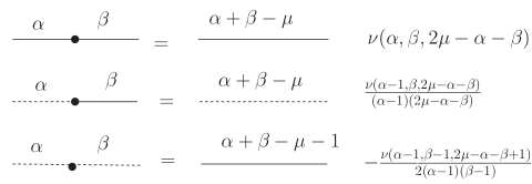
Figure 6: Products of two propagators are related to a single propagator. So, in a two-loop diagram,($\Sigma_{1}$ for example) inserting a point in one of the three propagators that connect to one internal vertex can make this vertex unique. The dotted lines denote fermions. Since we are dealing with chiral fermions, taking the trace in the third graph only produces one half the full result. $\nu$ is equal to $\nu(x_{1},x_{2},x_{3})=\pi\prod_{i=1}^{3}\alpha(x_{i})$.

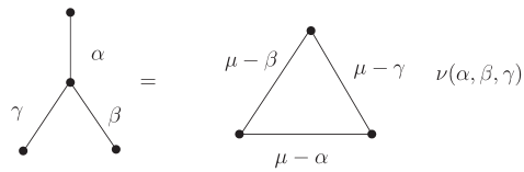
Figure 7: An identity that allows the integration of a unique vertex. Only bosonic propagators are shown. Similar identities with fermions can which are used in our calculation can be found in [20]

There are 11 diagrams needed for the calculation of $\eta$ at $1/D^{2}$. We designate them by $\Sigma$, $\Pi$, $\Phi$, $F$. The way to compute them was developed in [8, 15] for the bosonic graphs and extended to include fermionic graphs in [16, 17]. The main advantage of the method is that there is no need to explicitly evaluate any Feynman diagram. Here we will only give a few key observations that facilitate the evaluation of the diagrams. The first observation is that the chain of two propagators is equal to a propagator times a prefactor. Graphically this is shown in Fig 6, where $\nu(x_{1},x_{2},x_{3})=\pi^{\mu}\prod_{i=1}^{3}\alpha(x_{i})$. The third exponent $x_{3}$ is determined by the “uniqueness” [15] requirement $\sum_{i}x_{i}=2\mu$, for the bosonic graphs and $\sum_{i}x_{i}=2\mu-1$ if there are one or more fermion lines in the graph. An identity exists for a three point vertex, which is similarly related to a “unique” triangle, where now the uniqueness requirement is that $\sum_{i}x_{i}=\mu$. If there are one or more fermion lines the uniqueness changes to $\sum_{i}x_{i}=\mu+1$, and the results of [16] are unchanged in our case. There is no similar identity for a four point function, and for the (1,1) supersymmetric model that means that one has to retain the auxiliary field $F$. In computing the values at order $1/D^{2}$, $\chi$ is set to zero [15]. For a non-zero $\Delta$ the diagrams, for example the self energy of $\Psi$ designated $A$, lose their uniqueness. However one can subtract from $A$ a graph $B$ that has the same divergent substructure as $A$, but can be calculated for an arbitrary $\Delta$. So one has to compute $(A-B)+B$. Since $B$ can be calculated for arbitrary $\Delta$ and contains the divergence, one can evaluate $(A-B)$ at zero $\Delta$ when both diagrams become unique. A valuable first step in the calculation is the evaluation of all the self-energy graphs, which we will not include here since it was done in detail in [15, 17]. We just note that the most basic tool is the insertion of a point facilitated by the fact that we can write a propagator as a product of two. Then one can choose one of the exponents in such a way that the vertex that the propagator is attached to, becomes unique.

Appendix C Calculation of the graphs needed for $\eta_{2}$

We give the results for the various graphs occurring in the $1/D^{2}$ calculation. We only give the simple pole term and the constant term in an expansion in $\Delta$. The purely bosonic graphs were calculated in [15]. Compared to the calculation of the fermionic graphs in [20], there are differences that have to do with taking the trace of fermion loops, i.e. some factors of two in bosonic diagrams with fermion loops. Otherwise the calculation is almost identical. We find small discrepancies with [20] in some of the diagrams, mostly factors of $2$ and some minus signs. The most notable difference is $\Phi_{1}$, where the residue has a different denominator. We believe that our value is correct, since it leads to the same $\chi_{1}$ as the evaluations from the other equations (58).

$${B(x)=\psi(x)+\psi(\mu-x)}$$

(85)

$${\Sigma_{1}=\frac{2\pi^{2\mu}\alpha^{2}(\Delta_{S})\alpha(\Delta_{\sigma})}{\Delta\Gamma(\mu)}\left(1+\frac{\Delta}{2}\left[B(\Delta_{\sigma})-B(\Delta_{S})\right]\right)}$$

(86)

$${\Sigma_{2}=\frac{2\pi^{2\mu}\alpha^{2}(\Delta_{S})\alpha(\Delta_{\sigma}-1)}{\Delta\alpha(\Delta_{\sigma}-1)\Gamma(\mu)}\left(1+\frac{\Delta}{2}\left[B(\Delta_{\sigma}-1)-B(\Delta_{S})+\frac{1}{\Delta_{\sigma}-1}-\frac{1}{\Delta_{S}}\right]\right)}$$

(87)

$${\Sigma_{3}=\frac{2\pi^{4\mu}\alpha^{3}(\Delta_{S})\alpha^{3}(\Delta_{\sigma})\alpha(\mu+\Delta_{S}-\Delta_{\sigma})}{\Delta\Gamma(\mu)}\left(\frac{1}{2}+\Delta\left[B(\Delta_{\sigma})-B(\Delta_{S})\right]\right)}$$

(88)

$${{}\Sigma_{4}=\frac{\pi^{4\mu}\alpha^{3}(\Delta_{S})\alpha^{2}(\Delta_{\sigma}-1)\alpha(\Delta_{\sigma})\alpha(\Delta_{S}+\mu-\Delta_{\sigma})}{\Delta\Delta_{S}(\Delta_{S}+\mu-\Delta_{\sigma})(\Delta_{\sigma}-1)^{2}\Gamma(\mu)}}$$

(89)

$${\Pi_{1}=\frac{2\pi^{2\mu}\alpha^{2}(\Delta_{S})\alpha(\Delta_{\sigma})}{\Delta\Gamma(\mu)}\left(1+\Delta\left[B(\Delta_{\sigma})-B(\Delta_{S})\right]\right)}$$

(90)

$${\Pi_{2}=\frac{\pi^{4\mu}\alpha^{3}(\Delta_{S})\alpha^{3}(\Delta_{\sigma})\alpha(\Delta_{S}+\mu-\Delta_{\sigma})}{\Delta\Gamma(\mu)}\left(1+\Delta\left[4B(\Delta_{\sigma})-3B(\Delta_{S})-B(\mu+\Delta_{S}-\Delta_{\sigma})\right]\right)}$$

(91)

$${\Pi_{3}}$$

(92)

$${\Phi_{1}=-\frac{\pi^{2\mu}\alpha^{2}(\Delta_{S}-1)\alpha(\Delta_{\sigma})}{\Delta\Delta_{S}(\Delta_{S}-1)\Gamma(\mu)}\left(1+\Delta\left[B(\Delta_{\sigma})-B(\Delta_{S}-1)-\frac{1}{\Delta_{S}-1}\right]\right)}$$

(93)

$${\Phi_{2}=-\frac{\pi^{4\mu}\alpha^{3}(\Delta_{S})\alpha^{2}(\Delta_{\sigma}-1)\alpha(\Delta_{\sigma})\alpha(\Delta_{S}+\mu-\Delta_{\sigma})}{\Delta\Delta_{S}(\Delta_{S}+\mu-\Delta_{\sigma})(\Delta_{\sigma}-1)^{2}\Gamma(\mu)}}$$

(94)

$${F_{1}=-\frac{2\pi^{2\mu}\alpha^{2}(\Delta_{S})\alpha(\Delta_{\sigma}-1)}{\Delta\Delta_{S}(\Delta_{\sigma}-1)\Gamma(\mu)}\left(1+\Delta\left[B(\Delta_{\sigma}-1)-B(\Delta_{S})-\frac{1}{2\Delta_{S}}+\frac{1}{\Delta_{\sigma}-1}\right]\right)}$$

(95)

$${{}\qquad\qquad F_{2}=-\frac{\pi^{4\mu}\alpha^{3}(\Delta_{S})\alpha(\Delta_{\sigma})\alpha^{2}(\Delta_{\sigma}-1)\alpha(\Delta_{S}+\mu-\Delta_{\sigma})}{\Delta\Delta_{S}(\Delta_{S}+\mu-\Delta_{\sigma})(\Delta_{\sigma}-1)^{2}\Gamma(\mu)}}$$

(96)

Note that there is a similar three-loop diagram with $\Pi_{3}$ with the role of the $\Psi$, $u$ propagators interchanged. But it scales as $1/N^{3}$. A very useful identity for the evaluation of various quantities given in the text is $B(x)=B(\mu-x)$.

Appendix D Calculation of the graphs need for $\lambda_{2}$

In this section we give the formal expressions for the sums of the corrected diagrams (98)-(107), the values of the 43 individual diagrams that contribute (108)-(126), and finally the explicit form of the sums (127)-(135). Beforehand one has to define the functions appearing as

$${{}R_{1}=\psi^{\prime}(\mu-1)-\psi^{\prime}(\mu)}$$

(97)

where $\psi(z)=d\log\Gamma(z)/dz$.

$${\Sigma_{S}=2w^{2}\Sigma_{1Sa}+w^{2}\Sigma_{1Sb}-v^{2}\Sigma_{2S}+}$$

(98)

$${\Sigma_{\Psi}=-2v^{2}\Sigma_{2\Psi}-2Nv^{2}w(\Sigma_{4\Psi a}+\Sigma_{4\Psi b})}$$

(99)

$${\Sigma_{\sigma}=2w^{2}\Sigma_{1\sigma}+Nw^{3}(2\Sigma_{3\sigma a}+\Sigma_{3\sigma b})-2Nv^{2}w\Sigma_{4\sigma}}$$

(100)

$${\Sigma_{u}=-2v^{2}\Sigma_{2u}-2Nv^{2}w(\Sigma_{4ua}+\Sigma_{4ub})}$$

(101)

$${\Phi_{\Psi}=v^{2}\Phi_{1\Psi}+Nv^{2}w\Phi_{2\Psi}\quad\quad\Phi_{\sigma}=Nv^{2}w\Phi_{2\sigma}}$$

(102)

$${\Phi_{S}=2v^{2}\Phi_{1S}+2Nv^{2}w(\Phi_{1Sa}+\Phi_{2Sb})\quad\quad\Phi_{u}=2v^{2}\Phi_{1u}+Nv^{2}w\Phi_{2u}}$$

(103)

$${\Pi_{S}=4w^{2}\Pi_{1S}+Nw^{3}(4\Pi_{2Sa}+2\Pi_{2Sb})-4Nwv^{2}\Pi_{3S}}$$

(104)

$${\Pi_{\sigma}=w^{2}\Pi_{1\sigma}+2Nw^{3}\Pi_{2\sigma}\quad\quad\Pi_{\Psi}=-2Nwv^{2}\Pi_{3\Psi}\quad\quad\Pi_{u}=-2Nwv^{2}\Pi_{3u}}$$

(105)

$${F_{\Psi}=2v^{2}F_{1\Psi}+2Nv^{2}w2F_{2\Psi}\quad\quad F_{S}=2v^{2}F_{1S}+2Nv^{2}w(F_{2Sa}+F_{2Sb})}$$

(106)

$${F_{u}=v^{2}F_{1u}+Nv^{2}wF_{2u}\quad\quad F_{\sigma}=Nv^{2}wF_{2\sigma}}$$

(107)

There are 19 diagrams associated with the S-propagator and eight for the propagator of the other fields. The value of each graph of each graph is given below for completeness. The bosonic ones were calculated in [15], while similar to the fermionic ones were done in [19].

$${\Sigma_{1Sa}=\frac{\pi^{2\mu}}{(\mu-2)\Gamma^{2}(\mu)}\quad\quad\Sigma_{1Sb}=\frac{\pi^{2\mu}}{(\mu-2)^{2}\Gamma^{2}(\mu)}}$$

(108)

$${\Sigma_{2S}=-\frac{2(\mu+1)\pi^{2\mu}}{\mu(\mu-1)\Gamma^{2}(\mu)}\quad\quad\Sigma_{3Sa}=\frac{(\mu^{2}-3\mu+1)\Gamma(1-\mu)\pi^{4\mu}}{(\mu-2)^{3}\Gamma(\mu)\Gamma(2\mu-3)}}$$

(109)

$${\Sigma_{3Sb}=\frac{\pi^{4\mu}\Gamma(2-\mu)}{(2-\mu)\Gamma(\mu-1)\Gamma(2\mu-2)}\left(3R_{1}+\frac{2\mu-3}{(\mu-2)^{2}}\right)}$$

(110)

$${\Sigma_{3Sc}=\frac{\pi^{4\mu}\Gamma(4-\mu)}{(\mu-2)^{3}\Gamma(\mu-1)\Gamma(2\mu-4)}\quad\quad\Sigma_{4Sa}=\frac{2\pi^{4\mu}\Gamma(1-\mu)}{\Gamma(\mu)\Gamma(2\mu-2)}}$$

(111)

$${\Sigma_{4Sb}=-\frac{\pi^{4\mu}\Gamma(2-\mu)}{\Gamma(\mu)\Gamma(2\mu-2)}\left(3R_{1}+\frac{2\mu-3}{(\mu-1)(\mu-2)}\right)}$$

(112)

$${\Sigma_{4Sc}=\frac{2(\mu-3)(2\mu-3)\Gamma(1-\mu)\pi^{4\mu}}{(2-\mu)\Gamma(2\mu-2)\Gamma(\mu)}\quad\quad\Sigma_{2\Psi}=\frac{\pi^{2\mu}}{(\mu-1)\Gamma^{2}(\mu)}=-\Phi_{2S}}$$

(113)

$${\Sigma_{4\Psi a}=\frac{\pi^{4\mu}\Gamma(1-\mu)(2\mu^{2}-5\mu+1)}{2(\mu-2)\Gamma(\mu)\Gamma(2\mu-2)}=-\Phi_{2Sa}\quad\quad\Sigma_{4\Psi b}=\frac{\pi^{4\mu}3(\mu-3)\Gamma(2-\mu)R_{1}}{2(2-\mu)\Gamma(\mu)\Gamma(2\mu-2)}=-\Phi_{2Sb}}$$

(114)

$${\Sigma_{1\sigma}=\frac{\pi^{2\mu}(\mu^{2}-3\mu+1)}{(\mu-2)^{2}\Gamma^{2}(\mu)}=\Pi_{1S}\quad\quad\Sigma_{3\sigma a}=\frac{\pi^{4\mu}(2\mu^{2}-7\mu+4)\Gamma(1-\mu)}{(\mu-2)^{3}\Gamma(\mu)\Gamma(2\mu-3)}=\Pi_{2Sa}}$$

(115)

$${\Sigma_{3\sigma b}=\frac{3\pi^{4\mu}\Gamma(3-\mu)R_{1}}{(2-\mu)^{3}\Gamma(\mu-1)\Gamma(2\mu-2)}=\Pi_{2Sb}\quad\quad\Sigma_{4\sigma}=\frac{\pi^{4\mu}(2\mu-5)\Gamma(1-\mu)}{(\mu-2)\Gamma(\mu)\Gamma(2\mu-2)}=\Pi_{3S}}$$

(116)

$${\Sigma_{2u}=\frac{\pi^{2\mu}}{\Gamma^{2}(\mu)}\quad\quad\Sigma_{4ua}=\frac{\pi^{4\mu}(4\mu-9)\Gamma(1-\mu)}{2(\mu-2)\Gamma(\mu)\Gamma(2\mu-2)}=-F_{2sa}}$$

(117)

$${\Sigma_{4ub}=\frac{3\pi^{4\mu}\Gamma(2-\mu)R_{1}}{2(\mu-2)\Gamma(\mu)\Gamma(2\mu-2)}=-F_{2Sb}}$$

(118)

$${\Phi_{1S}=-\frac{\pi^{2\mu}}{(\mu-1)\Gamma^{2}(\mu)}\quad\quad\Phi_{1u}=\frac{\pi^{2\mu}\mu}{(1-\mu)\Gamma^{2}(\mu)}}$$

(119)

$${\Phi_{2u}=\frac{\pi^{4\mu}\Gamma(1-\mu)(4\mu^{2}-11m+5)}{2(1-\mu)(\mu-2)\Gamma(\mu)\Gamma(2\mu-2)}\quad\quad\Pi_{1\sigma}=\frac{3\pi^{2\mu}R_{1}}{(2-\mu)(2\mu-3)\Gamma^{2}(\mu-1)}}$$

(120)

$${\Pi_{2\sigma}=\frac{\pi^{4\mu}\Gamma(2-\mu)}{2(2-\mu)^{3}\Gamma(\mu-1)\Gamma(2\mu-1)}\left(6R_{1}-R_{2}-R_{3}^{2}+\frac{2(\mu-2)}{(\mu-1)(3\mu-2)}(R_{3}-\frac{1}{\mu-2})\right)}$$

(121)

$${\Pi_{3u}=-\frac{\Gamma(2-\mu)\pi^{4\mu}}{4(\mu-2)^{2}\Gamma(\mu)\Gamma(2\mu-2)}\left(6R_{1}^{2}-R_{2}-R_{3}^{2}+\frac{2R_{3}(\mu-2)-2}{(\mu-1)(2\mu-3)}\right)=-F_{2\sigma}}$$

(122)

$${\Pi_{3\Psi}=\frac{3\Gamma(2-\mu)\pi^{4\mu}R_{1}}{(2\mu-3)\Gamma(\mu)\Gamma(2\mu-1)}=\Phi_{2\sigma}\quad\quad F_{1\Psi}=\frac{\mu\pi^{2\mu}}{(1-\mu)\Gamma^{2}(\mu)}}$$

(123)

$${F_{2\Psi}=\frac{\pi^{4\mu}(4\mu^{2}-11\mu+5)\Gamma(1-\mu)}{2(1-\mu)(\mu-2)\Gamma(\mu)\Gamma(2\mu-2)}}$$

(124)

$${F_{1S}=-\frac{\pi^{2\mu}}{\Gamma^{2}(\mu)}\quad\quad F_{1u}=\frac{3(\mu-1)\pi^{2\mu}}{2(\mu-2)\Gamma^{2}(\mu)}}$$

(125)

$${F_{2u}=\frac{\pi^{4\mu}\Gamma(2-\mu)}{4(\mu-1)^{2}(\mu-2)^{2}\Gamma(\mu)\Gamma(2\mu-2)}\bigg{(}(\mu-1)(6R_{1}-R_{2}-R_{3}^{2})}$$

(126)

D.1 Summing up graphs

In this subsection we give the explicit values for the various sums appearing in the $\lambda_{2}$ calculation. We have omitted the $1/N^{2}$ factor that multiplies all of the diagrams so that the expression (66) for $\tilde{\lambda}_{2}$, does not contain any factors of $N$.

$${\frac{\Sigma_{S}}{\eta_{1}v_{1}}=-1+\frac{\mu+2}{\mu-1}+}$$

(127)

$${\Sigma_{\Psi}=-\eta_{1}v_{1}\left(\frac{\mu^{2}(\mu-2)(2\mu-3)}{\mu-1}+3(\mu-1)(\mu-3)R_{1}\right)=\Phi_{S}}$$

(128)

$${\Sigma_{\sigma}=-\eta_{1}v_{1}\left(\frac{\mu(3+\mu(3\mu-7))}{(\mu-1)^{2}}+3\mu(\mu-2)R_{1}\right)=\frac{\Pi_{S}}{2}}$$

(129)

$${\Sigma_{u}=\eta_{1}v_{1}(\mu(8-4\mu+3(\mu-1)R_{1})=F_{S}}$$

(130)

$${\Phi_{\sigma}=\eta_{1}v_{1}\frac{3\mu(\mu-1)(\mu-2)R_{1}}{2\mu-3}=(\Pi_{\Psi})/2}$$

(131)

$${\frac{\Phi_{u}}{\eta_{1}v_{1}}=1+6\mu-4\mu^{2}-\frac{1}{\mu-1}=-\frac{F_{\Psi}}{\eta_{1}v_{1}}}$$

(132)

$${\frac{\Pi_{\sigma}}{\eta_{1}v_{1}}=\left(\frac{3\mu(\mu-2)}{2(2\mu-3)}R_{1}-\frac{\mu}{\mu-1}\left[6R_{1}-R_{2}-R_{3}^{2}+\frac{2((\mu-2)R_{3}-1)}{(2\mu-3)(\mu-1)}\right]\right)}$$

(133)

$${\frac{\Pi_{u}}{\eta_{1}v_{1}}=\frac{\mu(\mu-1)}{\mu-2}\Big{(}6R_{1}-R_{2}-R_{3}^{2}+2\frac{(\mu-2)R_{3}-1}{(2\mu-3)(\mu-1)}\Big{)}=-\frac{2F_{\sigma}}{\eta_{1}v_{1}}}$$

(134)

$${\frac{F_{u}}{\eta_{1}v_{1}}=\frac{3}{4}\frac{\mu(\mu-1)}{\mu-2}+\frac{\mu}{4}\left(6R_{1}-R_{2}+R_{3}^{2}-\frac{4}{(\mu-1)^{2}}+\frac{2}{(2\mu-3)(\mu-1)}+\frac{2(\mu-2)}{2\mu-3}R_{3}\right)\,.}$$

(135)

References

- [1] J. J. Friess and S. S. Gubser, “Non-linear sigma models with anti-de Sitter target spaces,” hep-th/0512355.
- [2] J. M. Maldacena, “The large N limit of superconformal field theories and supergravity,” Adv. Theor. Math. Phys. 2 (1998) 231–252, hep-th/9711200.
- [3] S. S. Gubser, I. R. Klebanov, and A. M. Polyakov, “Gauge theory correlators from non-critical string theory,” Phys. Lett. B428 (1998) 105–114, hep-th/9802109.
- [4] E. Witten, “Anti-de Sitter space and holography,” Adv. Theor. Math. Phys. 2 (1998) 253–291, hep-th/9802150.
- [5] O. Aharony, S. S. Gubser, J. M. Maldacena, H. Ooguri, and Y. Oz, “Large N field theories, string theory and gravity,” Phys. Rept. 323 (2000) 183–386, hep-th/9905111.
- [6] A. Sen, “The heterotic string in arbitrary background field,” Phys. Rev. D32 (1985) 2102.
- [7] C. M. Hull and E. Witten, “Supersymmetric sigma models and the heterotic string,” Phys. Lett. B160 (1985) 398–402.
- [8] A. N. Vasiliev, Y. M. Pismak, and Y. R. Khonkonen, “1/N expansion: Calculation of the exponents and in the order for arbitrary number of dimensions,” Theor. Math. Phys. 47 (1981) 465–475.
- [9] A. M. Polyakov, “Interaction of Goldstone particles in two-dimensions. Applications to ferromagnets and massive Yang-Mills fields,” Phys. Lett. B59 (1975) 79–81.
- [10] E. Witten, “A supersymmetric form of the nonlinear sigma model in two-dimensions,” Phys. Rev. D16 (1977) 2991.
- [11] O. Alvarez, “Dynamical symmetry breakdown in the supersymmetric nonlinear sigma model,” Phys. Rev. D17 (1978) 1123.
- [12] I. Aref’eva, V. Krivoshchekov, and P. Medvedev, “1/N Perturbation theory and quantum conservation laws for the supersymmetric chiral field,” Theor. Math. Phys. 40 (1980) 565.
- [13] D. J. Gross and A. Neveu, “Dynamical symmetry breaking in asymptotically free field theories,” Phys. Rev. D10 (1974) 3235.
- [14] A. Zamolodchikov and A. Zamolodchikov, “Relativistic S-Matrix in two dimensions having O(N) isotopic Symmetry,” Nucl. Phys. B133 (1978) 525. Also JETP 26 (1977) 457.
- [15] A. N. Vasiliev, Y. M. Pismak, and Y. R. Khonkonen, “Simple method of calculating the critical indices in the expansion,” Theor. Math. Phys. 46 (1981) 104–113.
- [16] J. A. Gracey, “On the Beta function for sigma models with N=1 supersymmetry,” Phys. Lett. B246 (1990) 114–118.
- [17] J. A. Gracey, “Critical exponents for the supersymmetric sigma model,” J. Phys. A23 (1990) 2183–2194.
- [18] S.-k. Ma, “Critical Exponents above to O(1/n),” Phys. Rev. A7 (1973) 2172.
- [19] J. A. Gracey, “Probing the supersymmetric O(N) sigma model to : Critical exponent ,” Nucl. Phys. B352 (1991) 183–214.
- [20] J. A. Gracey, “Probing the supersymmetric O(N) sigma model to : Critical exponent ,” Nucl. Phys. B348 (1991) 737–756.
- [21] A. P. Foakes, N. Mohammedi, and D. A. Ross, “Three loop beta functions for the superstring and heterotic string,” Nucl. Phys. B310 (1988) 335.
- [22] A. P. Foakes, N. Mohammedi, and D. A. Ross, “Effective action and beta functions for the heterotic string,” Phys. Lett. B206 (1988) 57.
- [23] M. T. Grisaru, A. E. M. van de Ven, and D. Zanon, “Four loop divergences for the supersymmetric nonlinear sigma models in two-dimensions,” Nucl. Phys. B277 (1986) 409.
- [24] M. T. Grisaru, A. E. M. van de Ven, and D. Zanon, “Four loop function for the and supersymmetric nonlinear sigma model in two-dimensions,” Phys. Lett. B173 (1986) 423.
- [25] F. Wegner, “Four loop order beta function of nonlinear sigma models in symmetric spaces,” Nucl. Phys. B316 (1989) 663–678.
- [26] I. Jack, D. R. T. Jones, and N. Mohammedi, “The four loop metric beta function for the bosonic sigma model,” Phys. Lett. B220 (1989) 171.
- [27] I. Jack, D. R. T. Jones, and N. Mohammedi, “A four loop calculation of the metric beta function for the bosonic sigma model and the string effective action,” Nucl. Phys. B322 (1989) 431.
- [28] D. J. Gross and J. H. Sloan, “The quartic effective action for the heterotic string,” Nucl. Phys. B291 (1987) 41.
- [29] R. R. Metsaev and A. A. Tseytlin, “Curvature cubed terms in string theory effective actions,” Phys. Lett. B185 (1987) 52.
- [30] Y. Cai and C. A. Nunez, “Heterotic string covariant amplitudes and low-energy effective action,” Nucl. Phys. B287 (1987) 279.
- [31] A. A. Tseytlin, “Vector field effective action in the open superstring theory,” Nucl. Phys. B276 (1986) 391.
- [32] I. Jack, D. R. T. Jones, and D. A. Ross, “On the relationship between string low-energy effective actions and sigma model beta functions,” Nucl. Phys. B307 (1988) 130.
- [33] U. Ellwanger, J. Fuchs, and M. G. Schmidt, “The heterotic sigma model with background gauge fields,” Nucl. Phys. B314 (1989) 175.
- [34] U. Ellwanger, J. Fuchs, and M. G. Schmidt, “The heterotic sigma model in the presence of background gauge fields: three loop results,” Phys. Lett. B203 (1988) 244.
- [35] H. Osborn, “String theory effective actions from bosonic sigma models,” Nucl. Phys. B308 (1988) 629.
- [36] H. Osborn, “General bosonic sigma models and string effective actions,” Ann. Phys. 200 (1990) 1.
- [37] S. P. de Alwis, “Strings in background fields beta functions and vertex operators,” Phys. Rev. D34 (1986) 3760.
- [38] Y. Okabe and M. Oku, “1/N Expansion up to order 1/N**2. 3. Critical exponents gamma and nu for D = 3,” Prog. Theor. Phys. 60 (1978) 1287–1297.
- [39] I. R. Klebanov and A. M. Polyakov, “AdS dual of the critical O(N) vector model,” Phys. Lett. B550 (2002) 213–219, hep-th/0210114.
- [40] T. Leonhardt, A. Meziane, and W. Ruhl, “On the proposed AdS dual of the critical O(N) sigma model for any dimension ,” Phys. Lett. B555 (2003) 271–278, hep-th/0211092.
- [41] M. B. Green and J. H. Schwarz, “Anomaly cancelation in supersymmetric D=10 gauge theory and superstring theory,” Phys. Lett. B149 (1984) 117–122.
- [42] W. A. Bardeen and B. Zumino, “Consistent and covariant anomalies in gauge and gravitational theories,” Nucl. Phys. B244 (1984) 421.
- [43] E. Witten, “World-sheet corrections via D-instantons,” JHEP 02 (2000) 030, hep-th/9907041.