Solitonic generation of vacuum solutions in five-dimensional General Relativity

Abstract

We describe a solitonic solution-generating technique for the five-dimensional General Relativity. Reducing the five-dimensional problem to the four-dimensional one, we can systematically obtain single-rotational axially symmetric vacuum solutions. Applying the technique for a simple seed solution, we have previously obtained the series of stationary solutions which includes $S^{2}$-rotating black ring. We analyze the qualitative features of these solutions, e.g., conical singularities, closed timelike curves, and spacetime curvatures. We investigate the rod structures of seed and solitonic solutions. We examine the relation between the expressions of the metric in the prolate-spheroidal coordinates and in the C-metric coordinates.

I Introduction

In the recent years, finding exact solutions of higher-dimensional General Relativity has attracted much interest. There are several reasons for this. The string theory, which is a promising candidate of a quantum gravity theory, predicts that the spacetime has more than four dimensions. Furthermore the possibilities of the large or infinite extradimensions are proposed for solving the hierarchy problem Arkani-Hamed:1998rs ; Randall:1999ee . Also, the production of higher-dimensional black holes in future linear colliders is predicted based on these models Giddings:2001bu .

Although the uniqueness theorem has not been generalized to the higher dimensions yet, the studies of the spacetime structures in higher-dimensional General Relativity revealing the rich structure have been performed recently with great intensity. For example, several authors examined some qualitative features concerning the black hole horizon topologies in higher dimensions ref0 . This possibility of the variety of horizon topologies gives difficulty to the establishment of theorems analogous with the powerful uniqueness theorem in four dimensions. Also several exact solutions involving black holes were obtained in the higher-dimensional spacetime. The higher-dimensional generalization of the four-dimensional exact solutions were obtained for cases of the Schwarzschild and Reisner-Nordström black holes by Tangherlini Tangherlini:1963 and for the Kerr black hole by Myers and Perry refMP . Particularly in the five-dimensional case, several researchers have tried to search new exact solutions since the remarkable discovery of a rotating black ring solution with horizon topology $S^{1}\times S^{2}$ by Emparan and Reall ref1 . For example, the supersymmetric black rings ref2 and the black ring solutions under the influence of external fields ref3 are found. The systematical derivation of these solutions and some generalizations were examined by Yazadjiev Yazadjiev:2005hr . In addition the richness of the phase structure of Kaluza-Klein black holes have been discussed. Above all, the phases with and without Kaluza-Klein bubbles Witten:1981gj ; Elvang:2002br have been investigated energetically. (See Elvang:2004ny ; Elvang:2004iz and references therein.) Also the phase transition between black holes and black strings are widely investigated. (See, e.g., Kol:2004ww and references therein.) New geometrical structure of charged static black hole in the five-dimensional Einstein-Maxwell theory has been studied Ishihara:2005dp .

In this context a systematical search of possible solutions in higher dimensions　 is of great significance. In the four-dimensional General Relativity, the solution-generating techniques had been fully developed for the stationary and axisymmetric spacetime. These techniques were used for the systematical generations of solutions Stephani:2003tm , including the famous multi-Kerr solutions ref6 , since the discovery of Tomimatsu-Sato solutions ref5 . As in the four-dimensional case, the development of systematical ways of constructing new solutions would promote our understanding of the higher-dimensional General Relativity.

Using the fact that finding some class of five-dimensional solutions can be reduced to the four-dimensional problem Dereli:1977 ; Bruckman:1985yk ; Mazur:1987 , the present authors Mishima:2005id obtained a new class of five-dimensional stationary solutions by using a kind of Bäcklund transformation. In the analysis the formula given by Castejon-Amenedo and Manko ref7 were applied. (See also Gutsunaev:1988xh .) This method is promising in the point that we can easily perspect the property of the solution and obtain the exact expression of it. It was shown that the solutions obtained in Mishima:2005id include a single-rotational black ring solution with $S^{1}\times S^{2}$ event horizon topology which rotates in the azimuthal direction of $S^{2}$. This $S^{2}$-rotating black ring solution is important, especially when we try to find a double-rotational black ring solution, because it should be realized when we take a single-rotational limit of the double-rotational black ring. After the discovery of the solution, Figueras found a C-metric expression of $S^{2}$-rotating black ring solution Figueras:2005zp . Tomizawa et al. Tomizawa:2005wv showed that the same black ring solution is obtained by using the inverse scattering method refBZ , which has potential to produce more general solutions. This techniques was applied to the higher-dimensional theory of Kaluza-Klein compactifications several decades ago refKK . Recently it was applied to the five-dimensional static Einstein equation Koikawa:2005ia . Also this technique was used to rederive the five-dimensional Myers and Perry solution Pomeransky:2005sj . Using this technique and a matrix transformation of Ehlers type, solitonic solutions of five-dimensional string theory system were obtained Herrera-Aguilar:2003ui ; Herrera-Aguilar:2005sa .

In this paper we present a detailed explanation for the solution-generating technique used to derive the new solutions in the previous paper Mishima:2005id . In addition we analyze the qualitative features of the solutions including singular ones in detail. These solutions are generated from the five-dimensional Minkowski spacetime as a seed solution. Although the spacetimes found here have singular objects like closed timelike curves (CTC) and naked curvature singularities in general, a part of these solutions is a new class of black ring solutions whose rotational planes are different from those of Emparan and Reall’s. This black ring solution needs a conical singularity inside or outside the ring because the effect of rotation cannot compensate for the gravitational attractive force. The excess angle of the ring can be represented by mass and radius parameters. When we fix the mass and radius parameters, there is an upper limit of the rotational parameter of the ring.

We also study the rod structures ref8 ; refHAR of the seed solution and the corresponding solitonic solution to understand the relation between them. The rod structure analysis help us to find the seed solution for the solitonic solution we want to obtain. Recently the seed solution of Emparan and Reall’s $S^{1}$-rotating black ring has been obtained following this strategy Iguchi:2006rd . It has been reported that the $S^{1}$-rotating black ring solution is generated starting from the Levi-Civita metric by using the inverse scattering method Tomizawa:2006vp .

Particularly in the $S^{2}$-rotating black ring, the C-metric representation of the solution was obtained Figueras:2005zp . This representation is simple and suitable for the analysis of the solutions. In this paper we investigate the relation between these two expressions in the prolate-spheroidal and C-metric coordinates.

The plan of the paper is as follows. In Sec. II we describe the solution-generating technique used in this analysis. In Sec. III we denote the application of the technique for the simple seed solution. We analyze the properties of the solutions derived in the application in Sec. IV. In Sec. V we give a summary of this article.

II Solitonic solution-generating technique

In this section we write up the procedure for generating the axisymmetric solution in the five-dimensional General Relativity, which was applied to the generation of the single-rotational black ring solution whose rotational direction is different from the one of Emparan-Reall’s ring Mishima:2005id . In this approach we use the fact that the five-dimensional problem with some conditions can be reduced to a four-dimensional problem, which had been investigated elaborately several decade ago. As a result, we can use several well-established solution-generating techniques in the four dimensions to generate new five-dimensional solutions in a straightforward way. Also if we prepare various seed solutions for each applications, then we can obtain various kinds of new solutions even within the limitation of single-rotation.

The spacetimes which we considered satisfy the following conditions: (c1) five dimensions, (c2) asymptotically flat spacetimes, (c3) the solutions of vacuum Einstein equations, (c4) having three commuting Killing vectors including time translational invariance and (c5) having a single nonzero angular momentum component. Under the conditions (c1) – (c5), we can employ the following Weyl-Papapetrou metric form (for example, see the treatment in refHAR ),

$$ds^{2} = -e^{2U_{0}}(dx^{0}-\omega d\phi)^{2}+e^{2U_{1}}\rho^{2}(d\phi)^{2}+e^{2U_{2}}(d\psi)^{2}$$ (1)

$$+e^{2(\gamma+U_{1})}\left(d\rho^{2}+dz^{2}\right),$$

where $U_{0}$, $U_{1}$, $U_{2}$, $\omega$ and $\gamma$ are functions of $\rho$ and $z$. Then we introduce new functions $S:=2U_{0}+U_{2}$ and $T:=U_{2}$ so that the metric form (1) is rewritten into

$$ds^{2} = e^{-T}\left[-e^{S}(dx^{0}-\omega d\phi)^{2}+e^{T+2U_{1}}\rho^{2}(d\phi)^{2}\right.$$ (2)

$$\hskip 0.0pt\left.+e^{2(\gamma+U_{1})+T}\left(d\rho^{2}+dz^{2}\right)\right]+e^{2T}(d\psi)^{2}.$$

Using this metric form the Einstein equations are reduced to the following set of equations,

$${\bf\rm(i)}\quad\nabla^{2}T\,=\,0,$$

$${\bf\rm(ii)}\quad\left\{\begin{array}[]{ll}&\partial_{\rho}\gamma_{T}={\displaystyle\frac{3}{4}\,\rho\,\left[\,(\partial_{\rho}T)^{2}-(\partial_{z}T)^{2}\,\right]}\\[8.53581pt] &\partial_{z}\gamma_{T}={\displaystyle\frac{3}{2}\,\rho\,\left[\,\partial_{\rho}T\,\partial_{z}T\,\right],}\end{array}\right.$$

$${\bf\rm(iii)}\quad\nabla^{2}{{\mathcal{E}}}_{S}=\frac{2}{{{\mathcal{E}}}_{S}+{\bar{{\mathcal{E}}}}_{S}}\,\nabla{{\mathcal{E}}}_{S}\cdot\nabla{{\mathcal{E}}}_{S},$$

$${\bf\rm(iv)}\quad\left\{\begin{array}[]{ll}&\partial_{\rho}\gamma_{S}={\displaystyle\frac{\rho}{2({{\mathcal{E}}}_{S}+{\bar{{\mathcal{E}}}}_{S})}\,\left(\,\partial_{\rho}{{\mathcal{E}}}_{S}\partial_{\rho}{\bar{{\mathcal{E}}}}_{S}-\partial_{z}{{\mathcal{E}}}_{S}\partial_{z}{\bar{{\mathcal{E}}}}_{S}\,\right)}\\ &\partial_{z}\gamma_{S}={\displaystyle\frac{\rho}{2({{\mathcal{E}}}_{S}+{\bar{{\mathcal{E}}}}_{S})}\,\left(\,\partial_{\rho}{{\mathcal{E}}}_{S}\partial_{z}{\bar{{\mathcal{E}}}}_{S}+\partial_{\rho}{{\mathcal{E}}}_{S}\partial_{z}{\bar{{\mathcal{E}}}}_{S}\,\right)},\end{array}\right.$$

$${\bf\rm(v)}\quad\left(\partial_{\rho}\Phi,\,\partial_{z}\Phi\right)=\rho^{-1}e^{2S}\left(-\partial_{z}\omega,\,\partial_{\rho}\omega\right),$$

$${\bf\rm(vi)}\quad\gamma=\gamma_{S}+\gamma_{T},$$

$${\bf\rm(vii)}\quad U_{1}=-\frac{S+T}{2},$$

where $\Phi$ is defined through the equation (v) and the function $\mathcal{E_{S}}$ is defined by $\,{{\mathcal{E}}}_{S}:=e^{S}+i\,\Phi\,.$ The equation (iii) is exactly the same as the Ernst equation in four dimensions refERNST , so that we can call ${{\mathcal{E}}}_{S}$ the Ernst potential. The most nontrivial task to obtain new metrics is to solve the equation (iii) because of its nonlinearity. To overcome this difficulty we can however use the methods already established in the four-dimensional case. Here we use the method similar to the Neugebauer’s Bäcklund transformation Neugebauer:1980 or the HKX transformation Hoenselaers:1979mk , whose essential idea is that new solutions are generated by adding solitons to seed spacetimes.

To write down the exact form of the metric functions, we follow the procedure given by Castejon-Amenedo and Manko ref7 , in which they discussed a deformation of a Kerr black hole under the influence of some external gravitational fields. In the five-dimensional space time we start from the following form of a static seed metric

$$ds^{2} = e^{-T^{(0)}}\left[-e^{S^{(0)}}(dx^{0})^{2}+e^{-S^{(0)}}\rho^{2}(d\phi)^{2}\right.$$ (5)

$$\left.+e^{2\gamma^{(0)}-S^{(0)}}\left(d\rho^{2}+dz^{2}\right)\right]+e^{2T^{(0)}}(d\psi)^{2}.$$

For this static seed solution, $e^{S^{(0)}}$, of the Ernst equation (iii), a new Ernst potential can be written in the form

$${\cal E}_{S}=e^{S^{(0)}}\frac{x(1+ab)+iy(b-a)-(1-ia)(1-ib)}{x(1+ab)+iy(b-a)+(1-ia)(1-ib)},$$ (6)

where $x$ and $y$ are the prolate-spheroidal coordinates: $\,\rho=\sigma\sqrt{x^{2}-1}\sqrt{1-y^{2}},\ z=\sigma xy\,,$ with $\sigma>0$. The ranges of $x$ and $y$ are $1\leq x$ and $-1\leq y\leq 1$. The functions $a$ and $b$ satisfy the following simple first-order differential equations

$$(x-y)\partial_{x}a = a\left[(xy-1)\partial_{x}S^{(0)}+(1-y^{2})\partial_{y}S^{(0)}\right],$$

$$(x-y)\partial_{y}a = a\left[-(x^{2}-1)\partial_{x}S^{(0)}+(xy-1)\partial_{y}S^{(0)}\right],$$

$$(x+y)\partial_{x}b = -b\left[(xy+1)\partial_{x}S^{(0)}+(1-y^{2})\partial_{y}S^{(0)}\right],$$

$$(x+y)\partial_{y}b = -b\left[-(x^{2}-1)\partial_{x}S^{(0)}+(xy+1)\partial_{y}S^{(0)}\right].$$

The metric functions for the five-dimensional metric (2) are obtained by using the formulas shown by ref7 ,

$$e^{S} = e^{S^{(0)}}\frac{A}{B},$$ (8)

$$\omega = 2\sigma e^{-S^{(0)}}\frac{C}{A}+C_{1},$$ (9)

$$e^{2\gamma} = C_{2}(x^{2}-1)^{-1}Ae^{2\gamma^{\prime}},$$ (10)

where $C_{1}$ and $C_{2}$ are constants and $A$, $B$ and $C$ are given by

$$A:=(x^{2}-1)(1+ab)^{2}-(1-y^{2})(b-a)^{2},$$ (11)

$$B:=[(x+1)+(x-1)ab]^{2}+[(1+y)a+(1-y)b]^{2}\,,$$

(12)

$$C:=(x^{2}-1)(1+ab)[b-a-y(a+b)]$$

$$\hskip 25.6073pt+(1-y^{2})(b-a)[1+ab+x(1-ab)]\,.$$ (13)

The function $\gamma^{\prime}$ in Eq. (10) is a $\gamma$ function corresponding to the static metric,

$$ds^{2} = e^{-T^{(0)}}\left[-e^{2U^{\mbox{\tiny(BH)}}_{0}+S^{(0)}}(dx^{0})^{2}+e^{-2U^{\mbox{\tiny(BH)}}_{0}-S^{(0)}}\rho^{2}(d\phi)^{2}\right.$$

$$\left.+e^{2(\gamma^{\prime}-U^{\mbox{\tiny(BH)}}_{0})-S^{(0)}}\left(d\rho^{2}+dz^{2}\right)\right]+e^{2T^{(0)}}(d\psi)^{2},$$

where ${\displaystyle U_{0}^{\mbox{\tiny(BH)}}=\frac{1}{2}\ln\left(\frac{x-1}{x+1}\right)}$. And then the function $T$ is equals to $T^{(0)}$ and $U_{1}$ is given by the Einstein equation (vii).

Next we consider the solutions of the differential equations (II). At first, we examine the case of a typical seed function

$$S^{(0)}=\frac{1}{2}\ln\left[\,R_{d}+(z-d)\,\right],$$ (15)

where $R_{d}=\sqrt{\rho^{2}+(z-d)^{2}}$. The general seed function is composed of seed functions of this form. Note that the above function $S^{(0)}$ is a Newtonian potential whose source is a semi-infinite thin rod ref8 .

In this case we can confirm that the following $a$ and $b$ satisfy the differential equations (II),

$$a=l_{\sigma}^{-1}e^{2\phi_{d,\sigma}}\ ,\ \ \ b=-l_{-\sigma}e^{-2\phi_{d,-\sigma}}\ ,$$ (16)

where

$$\phi_{d,c}=\frac{1}{2}\ln\left[\,e^{-{\tilde{U}}_{d}}\left(e^{2U_{c}}+e^{2{\tilde{U}}_{d}}\right)\,\right].$$ (17)

Here the functions ${\tilde{U}}_{d}$ and $U_{c}$ are defined as ${\tilde{U}}_{d}:=\frac{1}{2}\ln\left[\,R_{d}+(z-d)\,\right]$ and $U_{c}:=\frac{1}{2}\ln\left[\,R_{c}-(z-c)\,\right]$. Because of the linearity of the differential equations (II) for $S^{(0)}$, we can easily obtain $a$ and $b$ which correspond to a general seed function if it is a linear combination of (15). See appendix A for this point.

The function ${\gamma}^{\prime}$ is defined from the static metric (LABEL:static_5), so that ${\gamma}^{\prime}$ obeys the following equations,

$$\partial_{\rho}{\gamma}^{\prime}=\frac{1}{4}\rho\left[(\partial_{\rho}S^{\prime})^{2}-(\partial_{z}S^{\prime})^{2}\right]+\frac{3}{4}\rho\left[(\partial_{\rho}T^{\prime})^{2}-(\partial_{z}T^{\prime})^{2}\right],$$ (18)

$$\partial_{z}{\gamma}^{\prime}=\frac{1}{2}\rho\left[\partial_{\rho}S^{\prime}\partial_{z}S^{\prime}\right]+\frac{3}{2}\rho\left[\partial_{\rho}T^{\prime}\partial_{z}T^{\prime}\right],$$ (19)

where the first terms are contributons from Eq. (iv) and the second terms come from Eq. (ii). Here the functions $S^{\prime}$ and $T^{\prime}$ can be read out from Eq. (LABEL:static_5) as

$$S^{\prime} = 2\,U^{(BH)}_{0}+S^{(0)},$$ (20)

$$T^{\prime} = T^{(0)}.$$ (21)

To integrate these equations we can use the following fact that, the partial differential equations

$$\partial_{\rho}{\gamma}^{\prime}_{cd} = \rho\left[\partial_{\rho}{\tilde{U}}_{c}\partial_{\rho}{\tilde{U}}_{d}-\partial_{z}{\tilde{U}}_{c}\partial_{z}{\tilde{U}}_{d}\right],$$ (22)

$$\partial_{z}{\gamma}^{\prime}_{cd} = \rho\left[\partial_{\rho}{\tilde{U}}_{c}\partial_{z}{\tilde{U}}_{d}+\partial_{\rho}{\tilde{U}}_{d}\partial_{z}{\tilde{U}}_{c}\right],$$ (23)

have the following solution,

$${\gamma}^{\prime}_{cd}=\frac{1}{2}{\tilde{U}}_{c}+\frac{1}{2}{\tilde{U}}_{d}-\frac{1}{4}\ln Y_{cd},$$ (24)

where $Y_{cd}:=R_{c}R_{d}+(z-c)(z-d)+\rho^{2}$. The general solution of $\gamma^{\prime}$ is given by the linear combination of the functions $\gamma^{\prime}_{cd}$.

III application for simple seed metric

Using the solution-generating technique described above, we have obtained a series of five-dimensional axisymmetric stationary solutions in the previous paper Mishima:2005id . In this section we retrace the analysis to derive the explicit form of the metric.

We adopt the five-dimensional Minkowski spacetime as a seed solution in this analysis. To obtain the solutions with sufficient variety, however, we add a freedom of one parameter to the seed metric and start from the following metric form,

$$ds^{2} = \,-(dx^{0})^{2}+\left(\sqrt{\rho^{2}+(z+{\lambda}\sigma)^{2}}-(z+{\lambda}\sigma)\right)d\phi^{2}+\left(\sqrt{\rho^{2}+(z+{\lambda}\sigma)^{2}}+(z+{\lambda}\sigma)\right)d\psi^{2}$$ (25)

$$+\frac{1}{2\,\sqrt{\rho^{2}+(z+{\lambda}\sigma)^{2}}}(d\rho^{2}+dz^{2})$$

$$= -(dx^{0})^{2}+\sigma\left(\sqrt{(x^{2}-1)(1-y^{2})+(xy+\lambda)^{2}}-(xy+{\lambda})\right)d\phi^{2}+\sigma\Biglb(\sqrt{(x^{2}-1)(1-y^{2})+(xy+{\lambda})^{2}}$$

$$+(xy+{\lambda})\Bigrb)d\psi^{2}+\frac{\sigma(x^{2}-y^{2})}{2\,\sqrt{(x^{2}-1)(1-y^{2})+(xy+{\lambda})^{2}}}\left[\frac{dx^{2}}{x^{2}-1}+\frac{dy^{2}}{1-y^{2}}\right],$$

where ${\lambda}$ is an arbitrary real constant. To construct ringlike solutions we have to take $\lambda>1$. By introducing the new coordinates $r$ and $\chi$:

$$\rho=r\,\chi,\ \ \ z=\frac{1}{2}(\chi^{2}-r^{2})-{\lambda}\sigma,$$

we can easily confirm that the above metric corresponds to the Minkowski spacetime,

$$ds^{2} = \,-(dx^{0})^{2}+(dr^{2}+r^{2}d\phi^{2})+(d\chi^{2}+\chi^{2}d\psi^{2}).$$ (26)

From Eq.(25), we can read the form of the functions $S$ and $T$ as seed functions,

$$S^{(0)}=T^{(0)} = {\tilde{U}}_{-\lambda\sigma}$$ (27)

$$= \frac{1}{2}\ln\left[\sqrt{\rho^{2}+(z+{\lambda}\sigma)^{2}}+(z+{\lambda}\sigma)\right]$$

$$= \frac{1}{2}\ln\Biglb[\sigma\left(\sqrt{(x^{2}-1)(1-y^{2})+(xy+\lambda)^{2}}\right.$$

$$\left.+(xy+{\lambda})\right)\Bigrb].$$

Using Eqs. (16) and (17) we obtain the functions $a$ and $b$,

$$a = {\alpha}\,\,\frac{(x-y+1+{\lambda})+\sqrt{x^{2}+y^{2}+2{\lambda}xy+({\lambda}^{2}-1)}}{\ 2\left[(xy+{\lambda})+\sqrt{x^{2}+y^{2}+2{\lambda}xy+({\lambda}^{2}-1)}\right]^{1/2}},$$

$$b = \beta\,\,\frac{\ 2\left[(xy+{\lambda})+\sqrt{x^{2}+y^{2}+2{\lambda}xy+({\lambda}^{2}-1)}\right]^{1/2}}{(x+y-1+{\lambda})+\sqrt{x^{2}+y^{2}+2{\lambda}xy+({\lambda}^{2}-1)}},$$

where ${\alpha}=2\sigma^{1/2}l^{-1}_{\sigma}$ and $\beta=-l_{-\sigma}/(2\sigma^{1/2})$.

Next we reduce the explicit expression of the $\gamma^{\prime}$. When we substitute the seed functions (27) into Eqs. (20) and (21), the functions $S^{\prime}$ and $T^{\prime}$ are obtained as

$$S^{\prime} = 2\,U^{(BH)}_{0}+S^{(0)}=2({\tilde{U}}_{\sigma}-{\tilde{U}}_{-\sigma})+{\tilde{U}}_{-{\lambda}\sigma}$$ (30)

$$T^{\prime} = T^{(0)}={\tilde{U}}_{-{\lambda}\sigma}.$$ (31)

As a result, the differential equations (18) and (19) become

$$\partial_{\rho}{\gamma}^{\prime} = \rho\left[(\partial_{\rho}{\tilde{U}}_{\sigma})^{2}-(\partial_{z}{\tilde{U}}_{\sigma})^{2}\right]+\rho\left[(\partial_{\rho}{\tilde{U}}_{-\sigma})^{2}-(\partial_{z}{\tilde{U}}_{-\sigma})^{2}\right]$$ (32)

$$+\rho\left[(\partial_{\rho}{\tilde{U}}_{-{\lambda}\sigma})^{2}-(\partial_{z}{\tilde{U}}_{-{\lambda}\sigma})^{2}\right]$$

$$-2\rho\left[\partial_{\rho}{\tilde{U}}_{\sigma}\partial_{\rho}{\tilde{U}}_{-\sigma}-\partial_{z}{\tilde{U}}_{\sigma}\partial_{z}{\tilde{U}}_{-\sigma}\right]$$

$$+\rho\left[\partial_{\rho}{\tilde{U}}_{\sigma}\partial_{\rho}{\tilde{U}}_{-{\lambda}\sigma}-\partial_{z}{\tilde{U}}_{\sigma}\partial_{z}{\tilde{U}}_{-{\lambda}\sigma}\right]$$

$$-\rho\left[\partial_{\rho}{\tilde{U}}_{-\sigma}\partial_{\rho}{\tilde{U}}_{-{\lambda}\sigma}-\partial_{z}{\tilde{U}}_{-\sigma}\partial_{z}{\tilde{U}}_{-{\lambda}\sigma}\right],$$

$$\partial_{z}{\gamma}^{\prime} = 2\rho\left[\partial_{\rho}{\tilde{U}}_{\sigma}\partial_{z}{\tilde{U}}_{\sigma}\right]+2\rho\left[\partial_{\rho}{\tilde{U}}_{-\sigma}\partial_{z}{\tilde{U}}_{-\sigma}\right]$$ (33)

$$+2\rho\left[\partial_{\rho}{\tilde{U}}_{-{\lambda}\sigma}\partial_{z}{\tilde{U}}_{-{\lambda}\sigma}\right]$$

$$-2\rho\left[\partial_{\rho}{\tilde{U}}_{\sigma}\partial_{z}{\tilde{U}}_{-\sigma}+\partial_{\rho}{\tilde{U}}_{-\sigma}\partial_{z}{\tilde{U}}_{\sigma}\right]$$

$$+\rho\left[\partial_{\rho}{\tilde{U}}_{\sigma}\partial_{z}{\tilde{U}}_{-{\lambda}\sigma}+\partial_{\rho}{\tilde{U}}_{-{\lambda}\sigma}\partial_{z}{\tilde{U}}_{\sigma}\right]$$

$$-\rho\left[\partial_{\rho}{\tilde{U}}_{-\sigma}\partial_{z}{\tilde{U}}_{-{\lambda}\sigma}+\partial_{\rho}{\tilde{U}}_{-{\lambda}\sigma}\partial_{z}{\tilde{U}}_{-\sigma}\right].$$

Now we divide $\gamma^{\prime}$ into the six parts as

$${\gamma}^{\prime}={\gamma}^{\prime}_{\sigma,\sigma}+{\gamma}^{\prime}_{-\sigma,-\sigma}+{\gamma}^{\prime}_{-\lambda\sigma,-\lambda\sigma}-2{\gamma}^{\prime}_{\sigma,-\sigma}+{\gamma}^{\prime}_{\sigma,-\lambda\sigma}-{\gamma}^{\prime}_{-\sigma,-\lambda\sigma},$$ (34)

where the each terms are the solutions of Eqs. (22) and (23). Finally, using the Eq. (24), we obtain the resulting form of $\gamma^{\prime}$ as

$${\gamma}^{\prime} = \frac{1}{2}\left({\tilde{U}}_{\sigma}-{\tilde{U}}_{-\sigma}\right)$$

$$+{\tilde{U}}_{-{\lambda}\sigma}-\frac{1}{2}\left(\ln R_{\sigma}+\ln R_{-\sigma}+\ln R_{-{\lambda}\sigma}\right)$$

$$+\frac{1}{4}\left(2\ln Y_{\sigma,-\sigma}-\ln Y_{\sigma,-{\lambda}\sigma}+\ln Y_{-\sigma,-{\lambda}\sigma}\right)-\frac{3}{4}\ln 2.$$

Consequently the functions which is needed to express the full metric are completely obtained. The full metric is expressed as

$$ds^{2} = -\frac{A}{B}\left[dx^{0}-\left(2\sigma e^{-S^{(0)}}\frac{C}{A}+C_{1}\right)d\phi\right]^{2}$$ (36)

$$+\frac{B}{A}e^{-2S^{(0)}}\sigma^{2}(x^{2}-1)(1-y^{2})(d\phi)^{2}$$

$$+e^{2S^{(0)}}(d\psi)^{2}+\frac{C_{2}\sigma}{\sqrt{2}(\lambda+1)}$$

$$\times\frac{B(\sqrt{(x^{2}-1)(1-y^{2})+(xy+\lambda)^{2}}+\lambda x+y)}{(x+1)\sqrt{(x^{2}-1)(1-y^{2})+(xy+\lambda)^{2}}}$$

$$\times\left(\frac{dx^{2}}{x^{2}-1}+\frac{dy^{2}}{1-y^{2}}\right).$$

Note that we have rewritten the second line of the metric (36) in the simpler form than the previous one. In the following, the constants $C_{1}$ and $C_{2}$ are fixed as

$$C_{1}=\frac{\,\,2\sigma^{1/2}\,{\alpha}\,\,}{1+{\alpha}\beta},\ \ \ C_{2}=\frac{1}{\sqrt{2}(1+{\alpha}\beta)^{2}},$$

to assure that the spacetime does not have global rotation and that the periods of $\phi$ and $\psi$ become $2\pi$ at the infinity, respectively. The metric (36) in the canonical coordinates $\rho$ and $z$ is given in appendix B.

IV Properties of solution

In this section we investigate the qualitative features of the solution derived in the previous section. Before the detailed explanations, we summarize the basic properties of it briefly. The spacetime described by this solution is axially symmetric, stationary, and, in general, asymptotically flat. It is expected that there is a ringlike local object as in FIG. 1. The parameters of $\lambda$ and $\sigma$ characterize the size and mass of the local object, respectively. While appropriate combinations of $\alpha$ and $\beta$ can be considered as the Kerr and the NUT parameters in four-dimensional case. Because of the existence of rotation, the spacetime has ergo-regions around the ringlike object. Also, there are closed timelike curves in general case, where the metric component $g_{\phi\phi}$ are negative. In fact the value of $g_{\phi\phi}$ can be negative around the inner disk of the ring at $1<x<\lambda$ and $y=-1$ as we will show in the subsection IV.5. If we demand $g_{\phi\phi}=0$ at $1<x<\lambda$ and $y=-1$, we obtain the following quadratic equation for $\beta$,

$$2\alpha\beta^{2}+(2+\alpha^{2}(\lambda+1))\beta+\alpha(\lambda-1)=0.$$ (37)

We can confirm that the one of the solution of this equation

$$\beta=-\frac{2+{\alpha}^{2}({\lambda}+1)-\sqrt{{\alpha}^{4}({\lambda}+1)^{2}-4{\alpha}^{2}({\lambda}-3)+4}}{4{\alpha}}$$ (38)

is the condition for $g_{\phi\phi}\geq 0$. Even in this case, there are conical singularities inside or outside the rings. The reason for this is that the effect of rotation cannot compensate for the gravitational attractive force.

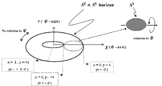
Figure 1: Schematic diagram of a local ringlike object which resides in the spacetime. Generally some singular behavior appears near the horizon.

In the rest of this section we discuss the physical properties of the solution in detail, including the results given in the previous paper Mishima:2005id .

IV.1 limits of solution

The solution (36) has several limits which assist our understanding of the nature of the solution. Direct generation of the limit solutions are given in appendix C. One of the most considerable limits is the Myers and Perry black hole with a single-rotation which is derived when we set $\lambda=1$ and $\beta=0$. In fact the metric has the following expression,

$$ds^{2} = -\frac{x-1-\alpha^{2}(1-y)}{x+1+\alpha^{2}(1+y)}\left(dx^{0}+2\sigma^{1/2}\alpha\frac{(1+\alpha^{2})(1-y)}{x-1-\alpha^{2}(1-y)}d\phi\right)^{2}+\sigma\frac{(x-1)(1-y)(x+1+\alpha^{2}(1+y))}{x-1-\alpha^{2}(1-y)}d\phi^{2}$$ (39)

$$+\sigma(x+1)(1+y)d\psi^{2}+\frac{\sigma}{2}(x+1+\alpha^{2}(1+y))\left(\frac{dx^{2}}{x^{2}-1}+\frac{dy^{2}}{1-y^{2}}\right)$$

$$= -\frac{p^{2}x+q^{2}y-1}{p^{2}x+q^{2}y+1}\left(dx^{0}+2\sigma^{1/2}\,\frac{q}{p}\,\frac{1-y}{p^{2}x+q^{2}y-1}d\phi\right)^{2}+\sigma\,\,\frac{p^{2}x+q^{2}y+1}{p^{2}x+q^{2}y-1}\,(x-1)\,(1-y)\,d\phi^{2}$$

$$+\sigma(x+1)\,(1+y)\,d\psi^{2}+{\sigma}\frac{p^{2}x+q^{2}y+1}{2p^{2}}\left[\frac{dx^{2}}{x^{2}-1}+\frac{dy^{2}}{1-y^{2}}\right],$$

where $p^{2}=1/({\alpha}^{2}+1)$ and $q^{2}={\alpha}^{2}/({\alpha}^{2}+1)$. Introduce new parameters $a_{0}$ and $m$, and new coordinates $\tilde{r}$ and $\theta$ through the relations,

$$p^{2}=\frac{4\sigma}{m^{2}},\ \ q^{2}=\frac{a_{0}^{2}}{m^{2}},$$ (40)

$$x=\frac{\tilde{r}^{2}}{2\sigma}-\lambda,\ y=\cos 2\theta,$$ (41)

so the metric (39) is transformed into

$$ds^{2} = -(1-\Delta)\left[dx^{0}+\frac{a_{0}\Delta\sin^{2}\theta}{1-\Delta}d\phi\right]^{2}$$ (42)

$$\hskip-8.5359pt\,+\,\frac{1}{1-\Delta}\left[\tilde{r}^{2}+(m^{2}-a_{0}^{2})\right]\sin^{2}\theta\,d\phi^{2}+\tilde{r}^{2}\cos^{2}\theta\,d\psi^{2}$$

$$\hskip-8.5359pt\,+\,(\tilde{r}^{2}+a_{0}^{2}\cos^{2}\theta)\left[d\theta^{2}+\frac{d\tilde{r}^{2}}{\tilde{r}^{2}-(m^{2}-a_{0}^{2})}\right],$$

where $\Delta:=m^{2}/(\tilde{r}^{2}+a_{0}^{2}\cos^{2}\theta)$. The line-element (42) is exactly the same form found by Myers and Perry.

Also this solution has a limit of a static black ring or a rotational black string when the condition (38) holds. The former case is realized when we take the limit ${\alpha}\rightarrow 0$. The parameter $\beta$ also approaches $0$ in this limit. Therefore the function $C$ and the constant $C_{1}$ become $0$ and then the spacetime approaches static one in this limit. In addition, the functions $A$ and $B$ become simple forms

$$A=x^{2}-1,~{}~{}~{}B=(x+1)^{2}.$$ (43)

So, the ergo-region and the CTC region do not appear in this spacetime obviously. The metric form of this limit becomes

$$ds^{2} = -\frac{x-1}{x+1}(dx^{0})^{2}+\sigma\frac{(x+1)^{2}(1-y^{2})}{\sqrt{(x^{2}-1)(1-y^{2})+(xy+\lambda)^{2}}+(xy+\lambda)}d\phi^{2}$$ (44)

$$+\sigma(\sqrt{(x^{2}-1)(1-y^{2})+(xy+\lambda)^{2}}-(xy+\lambda))d\psi^{2}$$

$$+\frac{\sigma}{2(\lambda+1)}\frac{(x+1)(\sqrt{(x^{2}-1)(1-y^{2})+(xy+\lambda)^{2}}+\lambda x+y))}{\sqrt{(x^{2}-1)(1-y^{2})+(xy+\lambda)^{2}}}\left(\frac{dx^{2}}{x^{2}-1}+\frac{dy^{2}}{1-y^{2}}\right).$$

This metric can be written in canonical coordinates as Eq. (106) in Appendix B.

The latter is realized when the parameter $\lambda$ goes to infinity under the condition: ${\alpha}=\tilde{{\alpha}}\times\sqrt{2/\lambda}$ with $-1<\tilde{{\alpha}}<1$. In this case $\beta$ goes to infinity like $-\tilde{\alpha}\times\sqrt{\lambda/2}$ while the product $\alpha\beta$ is finite and $-1<\alpha\beta=-\tilde{\alpha}^{2}<0$. As a result, the functions $a$ and $b$ approaches constants $\tilde{\alpha}$ and $-\tilde{\alpha}$, respectively. The $\psi$-$\psi$ component of the metric diverges except at $x=\infty$ and $y=-1$. To avoid this singular behavior we have to replace the angular coordinate $\psi$ with $\frac{\tilde{\psi}}{\sqrt{2\lambda}}$. Also we have to rescale $\phi$ as $\phi=\sqrt{2\lambda}\tilde{\phi}$. After these replacements, the metric can be rewtitten as

$$ds^{2} = -\frac{(1-{\tilde{\alpha}}^{2})^{2}(x^{2}-1)-4{\tilde{\alpha}}^{2}(1-y^{2})}{(x+1-{\tilde{\alpha}}^{2}(x-1))^{2}+4{\tilde{\alpha}}^{2}y^{2}}\left(dx^{0}+2\sigma^{1/2}\frac{2{\tilde{\alpha}}(1+{\tilde{\alpha}}^{2})((1-{\tilde{\alpha}}^{2})x+1+{\tilde{\alpha}}^{2})(1-y^{2})}{(1-{\tilde{\alpha}}^{2})^{2}((1-{\tilde{\alpha}}^{2})(x^{2}-1)-4{\tilde{\alpha}}^{2}(1-y^{2}))}d\tilde{\phi}\right)^{2}$$ (45)

$$+\sigma\frac{(x^{2}-1)(1-y^{2})(x+1-{\tilde{\alpha}}^{2}(x-1))^{2}+4{\tilde{\alpha}}^{2}y^{2}}{(1-{\tilde{\alpha}}^{2})^{2}(x^{2}-1)-4{\tilde{\alpha}}^{2}(1-y^{2})}d\tilde{\phi}^{2}+\sigma d\tilde{\psi}^{2}$$

$$+\sigma\frac{(x+1-{\tilde{\alpha}}^{2}(x-1))^{2}+4{\tilde{\alpha}}^{2}y^{2}}{2(1-{\tilde{\alpha}}^{2})^{2}}\left[\frac{dx^{2}}{x^{2}-1}+\frac{dy^{2}}{1-y^{2}}\right],$$

$$= -\frac{{\tilde{p}}^{2}x^{2}+{\tilde{q}}^{2}y^{2}-1}{({\tilde{p}}x+1)^{2}+{\tilde{q}}^{2}y^{2}}\left(dx^{0}+2\sigma^{1/2}\frac{2{\tilde{\alpha}}({\tilde{p}}x+1)(1-y^{2})}{{\tilde{p}}({\tilde{p}}^{2}x^{2}+{\tilde{q}}^{2}y^{2}-1)}d\tilde{\phi}\right)^{2}$$

$$+\sigma\frac{(x^{2}-1)(1-y^{2})({\tilde{p}}x+1)^{2}+{\tilde{q}}^{2}y^{2}}{{\tilde{p}}^{2}x^{2}+{\tilde{q}}^{2}y^{2}-1}d\tilde{\phi}^{2}+\sigma d\tilde{\psi}^{2}+\sigma\frac{({\tilde{p}}x+1)^{2}+{\tilde{q}}^{2}y^{2}}{2{\tilde{p}}^{2}}\left[\frac{dx^{2}}{x^{2}-1}+\frac{dy^{2}}{1-y^{2}}\right],$$

where ${\tilde{p}}=\frac{1-{\tilde{\alpha}}^{2}}{1+{\tilde{\alpha}}^{2}}$ and ${\tilde{q}}=\frac{2{\tilde{\alpha}}^{2}}{1+{\tilde{\alpha}}^{2}}$. This is just a rotational black string metric.

IV.2 asymptotic flatness

It should be noted that the solution-generating techniques developed in this study have an advantage that the resulting five-dimensional solutions hold asymptotic flatness if we adopt a five-dimensional asymptotically flat seed solution. This can be easily confirmed by the rod structure analysis, which will be discussed in the next subsection. If we take the asymptotic limit, $x\rightarrow\infty$, in the prolate-spheroidal coordinates, the metric form (36) approaches the asymptotic form of the Minkowski metric (25),

$$ds^{2} \sim -(dx^{0})^{2}+\sigma x(1-y)d\phi^{2}+\sigma x(1+y)d\psi^{2}$$ (46)

$$+\frac{\sigma}{2x}{dx^{2}}+\frac{\sigma x}{2(1-y^{2})}{dy^{2}}.$$

Also the asymptotic form of ${{\mathcal{E}}}_{S}$ near the infinity $x=\infty$ becomes

$${{\mathcal{E}}}_{S} = \tilde{r}\cos\theta\,\left[\,1\,-\,\frac{\sigma}{\tilde{r}^{2}}\,\frac{P({\alpha},\beta,{\lambda})}{(1+\alpha\beta)^{2}}\,+\cdots\right]$$

$$+2\,i\,\sigma^{1/2}\,\left[\,\frac{\alpha}{1+\alpha\beta}\,-\,\frac{2\sigma\cos^{2}\theta}{\tilde{r}^{2}}\,\frac{Q({\alpha},\beta,{\lambda})}{(1+\alpha\beta)^{3}}\,\,+\cdots\,\right],$$

where

$$P({\alpha},\beta,{\lambda}) = 4(1+\alpha^{2}-\alpha^{2}\beta^{2})$$

$$Q({\alpha},\beta,{\lambda}) = \alpha(2\alpha^{2}-{\lambda}+3)-2\alpha^{2}\beta^{3}$$

$$\hskip-11.38092pt-\beta\left[2(2\alpha\beta+1)(\alpha^{2}+1)+({\lambda}-1){\alpha}^{2}({\alpha}\beta+2)\right],$$

and we use the coordinates $(\tilde{r},\theta)$ through Eq. (41). This fact means that, even if ${\lambda}\neq 1$ or $\beta\neq 0$, the asymptotic form has the same asymptotic behavior as the case with ${\lambda}=1$ and $\beta=0$, i.e., the Myers-Perry black hole. From the asymptotic behavior, we can compute the mass parameter $m^{2}$ and rotational parameter $m^{2}a_{0}$:

$$m^{2}=\sigma\frac{P({\alpha},\beta,{\lambda})}{(1+\alpha\beta)^{2}},\ \ m^{2}a_{0}=4\sigma^{3/2}\frac{Q({\alpha},\beta,{\lambda})}{(1+\alpha\beta)^{3}}.$$ (48)

IV.3 rod structure analysis

We analyze the rod structure of the solution, which was studied for the higher-dimensional Weyl solutions by Emparan and Reall ref8 and for the nonstatic solutions by Harmark refHAR . The brief review of these methods are given in appendix D. We have four rods whose intervals are $z\in[-\infty,-\lambda\sigma]$, $[-\lambda\sigma,-\sigma]$, $[-\sigma,\sigma]$, and $[\sigma,\infty]$ at $\rho=0$ which correspond with $(x,y)\in\{\lambda\leq x,y=-1\}$, $\{1\leq x\leq\lambda,y=-1\}$, $\{x=1,-1\leq y\leq 1\}$, and $\{1\leq x,y=1\}$, respectively. The semi-infinite rod $[-\infty,-\lambda\sigma]$ has the direction ${\bf v}=(0,0,1)$. Therefore this rod corresponds to the fixed points of the $\psi$-rotation. The finite rod $[-\lambda\sigma,-\sigma]$ has the direction

$${\bf v} = (\Xi,1,0),$$

$$\Xi = \frac{2\sqrt{\sigma}(2\alpha\beta^{2}+(2+\alpha^{2}(\lambda+1))\beta+\alpha(\lambda-1))}{(1+\alpha\beta)(\lambda-1+\alpha\beta(\lambda+1))}.$$

(49)

It can be shown that this rod is spacelike. In general it does not correspond to the fixed points of the $\phi$-rotation. When the condition (37) holds, it becomes the fixed points of the $\phi$-rotation. The finite rod $[-\sigma,\sigma]$ has the direction

$${\bf v}=(1,\Omega,0),~{}~{}~{}\Omega=\frac{(1+\alpha\beta)((\lambda+1)\alpha-2\beta)}{2\sqrt{\sigma}((\lambda+1)\alpha^{2}+2)},$$ (50)

which corresponds to the region of time translational invariance. The semi-infinite rod $[\sigma,\infty]$ has the direction ${\bf v}=(0,1,0)$. Therefore this rod corresponds to the fixed points of the $\phi$-rotation. When the condition (37) holds, the topology of the event horizon is $S^{1}\times S^{2}$ for $\lambda>1$ as in Figure 1 because the rod $[-\sigma,\sigma]$ has the rods in the $\partial/\partial\phi$ direction on each side. Also the solution is free of the pathology of the Dirac-Misner string Elvang:2004xi in this case.

We show the schematic pictures of rod structures of the $S^{2}$-rotating black ring and its seed solution in Fig. 2. By the solution-generating transformation the segment $[-\sigma,\sigma]$ of semi-infinite spacelike rod of the seed, which corresponds to the fixed point of $\phi$-rotation, turns into the finite timelike rod with the direction (50). To indicate that this vector has nonzero $x^{0}$ and $\phi$ components, the rod is laid between $x^{0}$ and $\phi$ axes in Fig. 2. In general the segment $[-\lambda\sigma,-\sigma]$ also changes its direction from $\partial/\partial\phi$ to (49). We can see that the solitonic transformation keeps the existence of the two semi-infinite spacelike rods intact. This fact assures the asymptotic flatness of the obtained solution.

Figure 2: Schematic pictures of rod structures. The left panel shows the rod struture of Minkowski spacetime which is a seed of $S^{2}$-rotating black ring. The right panel shows the rod structure of the $S^{2}$-rotating black ring. The segment $[-\sigma,\sigma]$ of semi-infinite rod of the seed becomes finite timelike rod and changes its direction by the solution-generating transformation. Here we put the finite timelike rod between $x^{0}$ and $\phi$ lines because the corresponding eigenvector has nonzero $x^{0}$ and $\phi$ components. Note that the segment $[-\lambda\sigma,-\sigma]$ also changes its direction by the transformation in general.

IV.4 ergo region

As naturally expected from the presence of the rotation, the new solutions have ergo-regions where $g_{00}>0$. In fact, the 0-0 component of the metric (36) becomes positive near $x=1$ because the function $A$ becomes negative there. The form of this componet at $x=1$ is obtained as

$$g_{00}=\frac{((\lambda+1)\alpha-2\beta)^{2}(1-y^{2})}{8(\lambda+y)+(2\beta(1-y)+\alpha(\lambda+1)(1+y))^{2}}.$$ (51)

Figure 3 is the plot of $g_{00}$ for the region $1<x<4$ and $-1<y<1$ in a typical case of $(\alpha,\,\beta,\,\lambda)=(0.5,\,-0.195752,\,2)$ which satisfies the condition (38). There exists an ergo-region around the event horizon $x=1$.

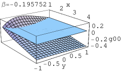
Figure 3: The behavior of $0$-$0$ component of the metric (36) in the case of $(\alpha,\,\beta,\,\lambda)=(0.5,\,-0.195752,\,2)$ . The region where the component function is above the level zero corresponds to the ergo-region.

Next we consider the relations between the ergo-region and the parameter $\alpha$. We plot the ergo-regions for the cases of $\alpha=0.5,0.7,0.9$ with $\lambda=2$ in FIG. 4. The values of $\beta$ are determined by the condition (38). The ergo-region of this ring spreads out towards the nonrotational axis $(x\geq\lambda,y=-1)$ of the ring as the value of $\alpha$ becomes large.

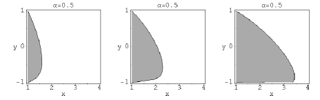
Figure 4: Ergo-regions for the cases of $\alpha=0.5,0.7,0.9$ with $\lambda=2$. The values of $\beta$ are determined by Eq. (38). In the shaded regions the values of $g_{00}$ are positive.

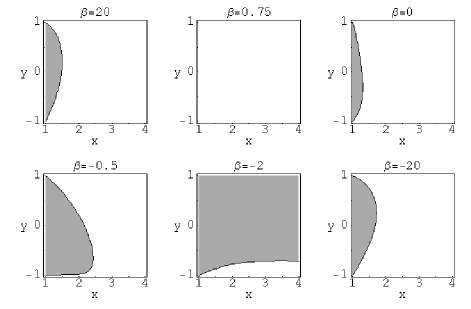
Figure 5: Ergo-regions for singular cases where $\alpha=0.5$ and $\lambda=2$. In the shaded regions the values of $g_{00}$ become positive. The values of $\beta$ do not satisfy Eq. (38). When $\beta=\frac{\alpha(1+\lambda)}{2}$, the ergo-region disappears.

For singular cases where Eq. (38) does not hold, we investigate the behaviors of $g_{00}$ for different values of $\beta$ as in FIG. 5. For the cases of large absolute values of $\beta$, the shapes of ergo-regions are similar with each other. There are two special cases, where $\beta=\frac{\alpha(1+\lambda)}{2}$ and $\beta=-\frac{1}{\alpha}$. The former case does not have ergo-regions. The latter case would be singular because the mass and rotational parameters diverges.

IV.5 closed timelike curve

There may exist closed timelike curves in this spacetime. It would be exist if the metric function $g_{\phi\phi}$ becomes negative. At first it can be easily shown that the value of $g_{\phi\phi}$ is zero at $y=1$. There is no harmful feature around there. However we can confirm the appearance of CTC from the fact that this component becomes

$$g_{\phi\phi}=-\frac{4\sigma(2\alpha\beta^{2}+(2+\alpha^{2}(\lambda+1))\beta+\alpha(\lambda-1))^{2}(x^{2}-1)}{(1+\alpha\beta)^{2}(8\beta^{2}(\lambda-x)+((\lambda-1)(x+1)+\alpha\beta(\lambda+1)(x-1))^{2})},$$ (52)

for the range $1<x<\lambda$ at $y=-1$. This value is always negative except when the parameters satisfy the condition (37). When $\lambda$ and $\alpha$ are given, the parameter $\beta$ must be

$$\beta=\beta_{+}=-\frac{2+{\alpha}^{2}({\lambda}+1)+\sqrt{{\alpha}^{4}({\lambda}+1)^{2}-4{\alpha}^{2}({\lambda}-3)+4}}{4{\alpha}},$$ (53)

or

$$\beta=\beta_{-}=-\frac{2+{\alpha}^{2}({\lambda}+1)-\sqrt{{\alpha}^{4}({\lambda}+1)^{2}-4{\alpha}^{2}({\lambda}-3)+4}}{4{\alpha}},$$ (54)

to satisfies the condition (37). Even in this case there can appear the CTC when the function $B$ becomes sufficiently small outside the ergo-region. We can show that the value of $B$ becomes zero at

$$x=\frac{(\lambda^{2}-1)\alpha^{2}-4\beta^{2}}{4\alpha\beta},~{}~{}~{}y=0.$$ (55)

For $\beta=\beta_{+}$, the coordinate value $x$ of (55) is in the range $x>1$. Therefore there appears singular behavior and $g_{\phi\phi}$ becomes negative in its neighborhood. While, when $\beta=\beta_{-}$, this singular behavior does not appear because the value of $x$ in (55) is less than 1. As a result, the condition (54) makes the singular structure of the spacetimes fairly mild as seen in the right panel of FIG. 6. The general case has regions where $g_{\phi\phi}$ becomes negative as in the left panel of FIG. 6.

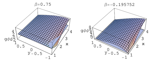
Figure 6: The behavior of $\phi$-$\phi$ component of the metric in the cases of $(\alpha,\,\beta,\,\lambda)=(0.5,0.75,2)$ and $(0.5,-0.195752,2)$ which satisfies the Eq. (38). The corresponding component in the right panel is always non-negative, while for the general case the component becomes negative near the horizon, which means the existence of CTC-regions.

We show the regions where $g_{\phi\phi}<0$ for different values of $\beta$ in FIG. 7. Note that the CTC-region can not touch with the event horizon $x=1$ except for the inner edge of the ring, $(x,y)=(1,-1)$. When the absolute values of $\beta$ are large, these regions become similar shapes with each other.

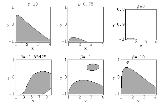
Figure 7: CTC-regions. In the shaded regions the values of $g_{\phi\phi}$ are negative. Note that the $y$-range of the right-upper panel and the $x$-range of the left-lower panel are different from the others. The left-lower panel corresponds to $\beta=\beta_{+}$.

IV.6 excess (deficit) angles

Even if the closed timelike curve does not exist, i.e., $\beta=\beta_{-}$, there exists a kind of strut structure in this spacetime. The reason for this is that the effect of rotation cannot compensate for the gravitational attractive force. The periods of the coordinates $\phi$ and $\psi$ should be defined as

$$\Delta\phi=2\pi\lim_{\rho\rightarrow 0}\sqrt{\frac{\rho^{2}g_{\rho\rho}}{g_{\phi\phi}}}~{}~{}~{}\mbox{and}~{}~{}~{}\Delta\psi=2\pi\lim_{\rho\rightarrow 0}\sqrt{\frac{\rho^{2}g_{\rho\rho}}{g_{\psi\psi}}}$$ (56)

to avoid a conical singularity. Both the value of $\Delta\psi$ for $x>\lambda$ and $y=-1$ and the value of $\Delta\phi$ for $y=1$, i.e., outside part of the $\phi$-axis-plane, are $2\pi$. While the period of $\phi$ inside the ring can be defined only when the condition (37) holds. In this case the period becomes

$$\Delta\phi=2\pi\frac{\lambda-1+(\lambda+1)\alpha\beta}{\sqrt{\lambda^{2}-1}(1+\alpha\beta)},$$ (57)

which is less than $2\pi$ for $\beta=\beta_{-}$ and larger than $2\pi$ for $\beta=\beta_{+}$. Hence, two-dimensional disklike struts, which appear in the case of static black rings ref8 , are needed to prevent the collapse of the $S^{2}$-rotating black rings.

We have introduced four parameters $\lambda$, $\sigma$, $\alpha$ and $\beta$ in our analysis. Also, we need the condition (38) for the disappearance of CTC regions. As a result there are three independent parameters for the $S^{2}$-rotating black ring. Here we take $\lambda$, $m$ and

$$h:=\frac{\lambda-1+(\lambda+1)\alpha\beta}{\sqrt{\lambda^{2}-1}(1+\alpha\beta)}$$ (58)

as these physical parameters. From Eqs. (37), (48) and (58) we can obtain the relations between these parameters and the other parameters $\sigma$, $\alpha$ and $\beta$ as

$$\sigma = \frac{m^{2}h}{2\sqrt{\lambda^{2}-1}(1-h^{2})},$$ (59)

$$\alpha = \pm\sqrt{\frac{2}{h(\lambda+1)}\frac{\sqrt{\lambda-1}-h\sqrt{\lambda+1}}{\sqrt{\lambda+1}-h\sqrt{\lambda-1}}},$$ (60)

$$\beta = \mp\sqrt{\frac{h(\lambda-1)}{2}\frac{\sqrt{\lambda-1}-h\sqrt{\lambda+1}}{\sqrt{\lambda+1}-h\sqrt{\lambda-1}}}.$$ (61)

The condition that the parameters $\alpha$ and $\beta$ should be real is

$$0<h<\sqrt{\frac{\lambda-1}{\lambda+1}}<1$$ (62)

or

$$h>\sqrt{\frac{\lambda+1}{\lambda-1}}>1.$$ (63)

The former case corresponds to the case of $\beta=\beta_{-}$and the latter to $\beta=\beta_{+}$. Therefore the period of $\phi$ inside the ring is always larger than $2\pi$ when the condition $\beta=\beta_{+}$ holds which corespond to the left-lower panel of FIG. 7. It should be noted that the mass parameter $m^{2}$ is negative in this case.

IV.7 maximal rotation limit

In this subsection we investigate the rotational parameter $a_{0}$ for the $S^{2}$-rotating black ring. The rotational parameter $a_{0}$ in Eq. (48) can be rewritten by using the parameters $\lambda$, $m$ and $h$ as

$$\frac{a_{0}^{2}}{m^{2}}=\frac{1-h}{1+h}-\frac{2h}{1-h^{2}}\left(\sqrt{\frac{\lambda^{2}}{\lambda^{2}-1}}-1\right).$$ (64)

When we fix the parameters $m$ and $h$, the rotational parameter increases uniformly according to the value of $\lambda$ and has a maximum value

$${a_{0}}_{max}=\sqrt{\frac{m^{2}(1-h)}{1+h}}.$$ (65)

The parameter $\lambda$ diverges at the maximum of $a_{0}$, while $\sigma$ goes to $0$ with keeping the value of $\lambda\sigma$ finite. Then the physical size of the ring is kept finite. The parameter $\alpha$ goes to $0$ at the maximum of $a_{0}$, while $\beta$ diverges to infinity. The parameters behave around the maximum of $a_{0}$ as

$$\sigma\sim\frac{m^{2}h}{2\lambda(1-h^{2})},~{}~{}~{}~{}~{}\alpha\sim\pm\sqrt{\frac{2}{h\lambda}},$$

$$\beta\sim\mp\sqrt{\frac{h\lambda}{2}},~{}~{}~{}~{}~{}1+\alpha\beta\sim\frac{2}{\lambda(1-h)}.$$ (66)

When we take this limit, we have to redefine the coordinate $x$ as, for example, $\tilde{x}-1=(x-1)/\lambda$ to extract the regular form of the solution.

In FIG. 8, we plot the values of $g_{\psi\psi}$ of the event horizon at $y=-1$ (inner edge), $y=0$ (middle) and $y=1$ (outer edge). Here we set the parameters as $m^{2}=3$ and $h=0.5$. The circumferences of the inner and the outer edge of the ring approach each other as the parameter $a_{0}$ becomes large. As we will see in IV.9, the event horizon degenerates at the maximum of $a_{0}$. Then we call this limit the extreme limit of the solution. In fact the rotational parameter ${a_{0}}_{max}$ equals the mass parameter $m$ when we take the five-dimensional Kerr black hole limit $h\rightarrow 0$.

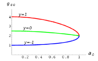
Figure 8: Plots of $\psi$-$\psi$ components of the $S^{2}$-rotating black ring for $a_{0}$ with $m^{2}=3$ and $h=0.5$. Upper, middle, and lower lines correspond with outer edge $(y=1)$, middle $(y=0)$ and inner edge $(y=-1)$ of the ring, respectively.

IV.8 curvature invariants

In this section we consider the possibility of the naked curvature singularity. Here we examine the scalar curvature

$$K = R_{ijkl}R^{ijkl},$$ (67)

which is usually called Kretchman invariant.

The rod structure analysis shows that the solution satisfies the necessary condition for the absence of the curvature singularity on the $z$-axis. It was shown in the above, however, that the function $B$ becomes zero for some cases. The curvature singularity appears at the point where $B=0$. We plot $K$ for the four representative cases in FIG. 9. The left-upper panel corresponds to the case of $\beta=\beta_{-}$ and $\lambda>1$. There cannot be seen a curvature singularity in this plot. The right-upper panel corresponds to the case of $\beta=\beta_{+}$ and $\lambda>1$. We can see that the value of curvature grows disastrously around the point where $B=0$ in this plot.

When $\lambda=1$ there appears a directional curvature singularity. For the singular case $\beta\neq\beta_{-}=0$, the Kretchman invariant diverges at $x=1$ as

$$K\propto\frac{72\beta^{4}}{(1+\alpha\beta)^{4}\sigma^{2}(x-1)^{4}}$$ (68)

along the plane $y=-1$. While this value is finite when we approach $y=-1$ on the event horizon $x=1$,

$$K=\frac{9(1+\alpha\beta)^{4}}{2\beta^{4}\sigma^{2}}.$$ (69)

The right-lower panel of FIG. 9 shows the behavior $K$ of this case. For the regular case $\beta=\beta_{-}=0$, there does not appear curvature singularity at $x=1$ and $y=-1$ and the value of $K$ is obtained as

$$K=\frac{9(1+\alpha^{2})^{2}}{2\sigma^{2}}.$$ (70)

The left-lower panel of FIG. 9 shows the behavior $K$ of single-rotational black hole.

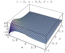
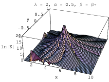
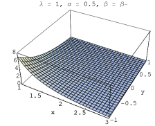
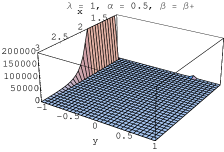
Figure 9: Plots of Kretchman Invariants for the cases of $(\lambda,\alpha,\beta,)=(2,0.5,\beta_{-})$, $(2,0.5,\beta{+})$, $(1,0.5,\beta{+})$, and $(1,0.5,\beta{-})$. In the right-upper panel we plot the value of $\ln|K|$. We can see that $K$ grows disastrously around the point where $B=0$.

IV.9 C-metric expression

The metric (36) is rewritten by the C-metric coordinates Figueras:2005zp as

$$ds^{2} = -\frac{H(\lambda_{c},v,u)}{H(\lambda_{c},u,v)}\left[dx^{0}-\frac{\lambda_{c}a_{c}v(1-u^{2})}{H(\lambda_{c},v,u)}d\bar{\phi}\right]^{2}$$ (71)

$$+\frac{R_{c}^{2}}{(u-v)^{2}}H(\lambda_{c},u,v)\left[-\frac{dv^{2}}{(1-v^{2})F(\lambda_{c},v)}\right.$$

$$\left.-\frac{(1-v^{2})F(\lambda_{c},u)}{H(\lambda_{c},u,v)}d\bar{\psi}^{2}+\frac{du^{2}}{(1-u^{2})F(\lambda_{c},u)}\right.$$

$$\left.+\frac{(1-u^{2})F(\lambda_{c},v)}{H(\lambda_{c},v,u)}d\bar{\phi}^{2}\right],$$

where

$$F(\lambda_{c},\xi)=1+\lambda_{c}\xi+\left(\frac{a_{c}\xi}{R_{c}}\right)^{2},$$

$$H(\lambda_{c},\xi_{1},\xi_{2})=1+\lambda_{c}\xi_{1}+\left(\frac{a_{c}\xi_{1}\xi_{2}}{R_{c}}\right)^{2},$$ (72)

and $-1<u<1$ and $-\infty<v<-1$. Here we give the relation between the prolate-spheroidal coordinates $(x,y)$ and the C-metric coordinates $(u,v)$. After a rather lengthy calculation, the metric (36) written by the prolate-spheroidal coordinates can be transformed into the expression (71) by using the following coordinate transformations,

$$x = \frac{2(u-v_{i})(v-v_{h})}{(u-v)(v_{h}-v_{i})}+1$$ (73)

$$y = \frac{uv-1}{u-v},$$ (74)

$$\phi = \frac{a_{c}\sqrt{(1+v_{h})(1+v_{i})}}{R_{c}}\bar{\phi},$$ (75)

$$\psi = \frac{a_{c}\sqrt{(1+v_{h})(1+v_{i})}}{R_{c}}\bar{\psi},$$ (76)

where

$$v_{h} = \frac{R_{c}^{2}}{2a_{c}^{2}}\left[-\lambda_{c}+\sqrt{\lambda_{c}^{2}-\frac{4a_{c}^{2}}{R_{c}^{2}}}\right]$$ (77)

$$v_{i} = \frac{R_{c}^{2}}{2a_{c}^{2}}\left[-\lambda_{c}-\sqrt{\lambda_{c}^{2}-\frac{4a_{c}^{2}}{R_{c}^{2}}}\right].$$ (78)

In addition the relation between the parameters $(\sigma,\lambda,\alpha,\beta)$ and $(R_{c},\lambda_{c},a_{c})$,

$$\sigma = \frac{R_{c}^{2}(v_{h}-v_{i})}{2(1+v_{h})(1+v_{i})}$$ (79)

$$\lambda = \frac{v_{h}v_{i}-1}{v_{h}-v_{i}}$$ (80)

$$\alpha = -\frac{\sqrt{2(v_{h}-v_{i})}}{v_{i}+1}$$ (81)

$$\beta = \frac{v_{h}+1}{\sqrt{2(v_{h}-v_{i})}},$$ (82)

should be used there. We can easily confirm that the no CTC condition $\beta=\beta_{-}$ is satisfied. Also, when the event horizon degenerates, $v_{h}=v_{i}$, the parameters show the same behavior as the case of maximum rotation Eq. (66). Inversely the parameters $\lambda_{c}$, $R_{c}^{2}$ and $a_{c}^{2}$ can be written as

$$\lambda_{c} = \frac{\lambda-1-(\lambda+1)\alpha^{2}\beta^{2}}{(\lambda(1+\alpha\beta)-1)(\lambda(1+\alpha\beta)+\alpha\beta)}$$ (83)

$$= \frac{2\sqrt{\lambda^{2}-1}(1-h^{2})}{(\sqrt{\lambda-1}+h\sqrt{\lambda+1})(\sqrt{\lambda+1}+h\sqrt{\lambda-1})}$$

$$R_{c}^{2} = -\frac{4\sigma\beta}{\alpha}$$ (84)

$$= \frac{m^{2}h^{2}}{1-h^{2}}$$

$$a_{c}^{2} = \frac{4\sigma\beta^{2}}{(\lambda(1+\alpha\beta)-1)(\lambda(1+\alpha\beta)+\alpha\beta)}$$

$$= \frac{m^{2}h^{2}}{1-h^{2}}\frac{(\sqrt{\lambda-1}-h\sqrt{\lambda+1})(\sqrt{\lambda+1}-h\sqrt{\lambda-1})}{(\sqrt{\lambda-1}+h\sqrt{\lambda+1})(\sqrt{\lambda+1}+h\sqrt{\lambda-1})}.$$

By using Eqs. (58) and (84) we can rewrite Eq. (57) as

$$\Delta\phi=2\pi h=\frac{2\pi}{\sqrt{1+\frac{m^{2}}{R_{c}^{2}}}}.$$ (86)

Therefore the period of $\phi$ is determined only by the ratio of the mass parameter $m$ to the radius parameter $R_{c}$.

In FIG. 10 we present schematic pictures for the relations between $(x,y)$ and $(r,\chi)$ coordinates and between $(u,v)$ and $(r,\chi)$ coordinates. Here we use the relations

$$\chi^{2}=\sigma(\sqrt{(x^{2}-1)(1-y^{2})+(xy+\lambda)^{2}}+xy+\lambda),~{}~{}~{}$$ (87)

$$r^{2}=\sigma(\sqrt{(x^{2}-1)(1-y^{2})+(xy+\lambda)^{2}}-xy-\lambda).$$ (88)

The lines of $u=$const. and $v=$const. are denser than $x$ and $y$ near the inner edge of the horizon.

Figure 10: The contour lines of $x$, $y$, $u$ and $v$ in $\chi-r$ plane. In the left panel, the solid lines and the dotted lines are $x=$ const. and $y=$ const. lines respectively. In the right panel, the solid lines and the dotted lines are $u=$ const. and $v=$ const. lines respectively.

V summary

In this paper we have described the solution-generating technique for the Einstein equation of five-dimensional General Relativity. Using this method we can systematically construct axisymmetric stationary solutions with asymptotic flatness. If we prepare various seed solutions, we can obtain different kinds of new solutions with the single-rotation. In our analysis we adopted the procedure given by Castejon-Amenedo and Manko to derive the exact form of the metric functions.

For the application of the method, we adopted the Minkowski spacetime as the simplest seed solution. Although the seed solution we adopted is so simple, the obtained series of the solutions has scientific importance. It includes two important limits, the Myers and Perry single-rotational black hole and the rotational black string. More significantly, the part of the series should be one single-rotational limit of an undiscovered double-rotational black ring which has the Emparan-Reall’s black ring as another limit.

We have examined the qualitative features of the solutions in detail. Generally, there are ergo-regions around the local black objects because of the rotation. In addition, there exist regions where the metric function $g_{\phi\phi}$ becomes negative. In these regions closed timelike curves can be exist. However, we have confirmed that there is no CTC region when the condition $\beta=\beta_{-}$ holds. Even in this case, the conical singularity is inevitable inside or outside the ring. Therefore we need the strut structure inside the ring because the periods of $\phi$ inside the ring is always smaller than those of $\phi$ outside the ring and of $\psi$. In addition we have shown that there is an upper limit of the rotation parameter $a_{0}$ when we fix the mass parameter $m$ and the radius parameter $R_{c}$. When the condition $\beta=\beta_{+}$ holds, we can also define the period of $\phi$ inside the ring. In this case there is positive deficit angles inside the ring in contrast to the case of $\beta=\beta_{-}$. We have investigated the behavior of the curvature invariant. This variable is finite when the condition $\beta=\beta_{-}$ holds and can diverge where $B=0$ for another cases. We have also shown that there is a directional curvature singularity for the case of $\lambda=1$.

By the rod structure analysis we have understood the relation between the seed and the obtained solutions. By analogy of this relation we can obtain a seed of the $S^{1}$-rotating black ring solution Iguchi:2006rd .

Finally, we derived the relations between the prolate-spheroidal coordinates and the C-metric coordinates which was derived by Figueras Figueras:2005zp . We confirmed the equivalence between the metric (36) with the condition $\beta=\beta_{-}$ and the expression given by Figueras.

In the method presented here we can also adopt other seed spacetimes, so that we can generate some new solutions. Although the solution obtained here has some pathologies including inevitable one, i.e., conical singularities, we can expect to obtain the new solution without these pathologies by an adequate seed metric as in the case of the $S^{1}$-rotating black ring which is reduced from the seed of Wick rotated C-metric solution Iguchi:2006rd . However it should be noticed that the method introduced here cannot be used for the solution generation of double-rotational black rings because of the metric form (1). For this purpose other methods may be used. One of the powerful tools would be the inverse scattering method refBZ .

Appendix A Neugebauer and Kramer representation

To derive the potential functions $a$ and $b$, it is convenient to use the Neugebauer and Kramer’s powerfull representation for Ernst potential Stephani:2003tm . Adding the $2N$ solitons to a static seed potential ${\cal E}^{(0)}$, the new Ernst potential is given by

$${\cal E}={{\cal E}^{(0)}}\frac{\det\left(\frac{{\alpha}_{p}R_{p}-{\alpha}_{q}R_{q}}{K_{p}-K_{q}}-1\right)}{\det\left(\frac{{\alpha}_{p}R_{p}-{\alpha}_{q}R_{q}}{K_{p}-K_{q}}+1\right)}$$ (89)

where $p=1,3,\dots,2N-1$, $q=2,4,\dots,2N$ and $R_{j}=\sqrt{\rho^{2}+(z-K_{j})^{2}}$. The function ${\alpha}_{j}$ is given by

$${\alpha}_{j}=\frac{l_{j}+ie^{2\phi_{j}}}{l_{j}-ie^{2\phi_{j}}}\,.$$ (90)

Here the quantity $l_{j}$ is an integral constant, and the function $\phi_{j}$ obeys the following Riccati equations,

$$d\phi_{j}=\frac{1}{2}\left[\,\,\left(\gamma_{j}\right)^{1/2}\partial_{\zeta}\ln{\cal E}^{(0)}d\zeta+\left(\gamma_{j}\right)^{-1/2}\partial_{\bar{\zeta}}\ln{\cal E}^{(0)}d\bar{\zeta}\,\,\right]\,,$$ (91)

where $\zeta=\rho+iz$, and $\gamma_{j}=(K_{j}-i\bar{\zeta})/(K_{j}+i\zeta)$. For the case of $\ln{\cal E}^{(0)}=\frac{1}{2}\ln\left[\,R_{d}+(z-d)\,\right]$, the function $\phi_{j}$ is given by

$$\phi_{j}=\phi_{d,j}=\frac{1}{2}\ln\left[\,e^{-{\tilde{U}}_{d}}\left(e^{2U_{j}}+e^{2{\tilde{U}}_{d}}\right)\,\right],$$ (92)

where ${\tilde{U}}_{d}:=\frac{1}{2}\ln\left[\,R_{d}+(z-d)\,\right]$ and $U_{j}:=\frac{1}{2}\ln\left[\,R_{j}-(z-K_{j})\,\right]$.

Next we consider the relation between the Ernst potentials (6) and (89). The parameter $K_{1}$ and $K_{2}$ are set to $\sigma$ and $-\sigma$, respectively so that the useful expression,

$$R_{\sigma}=\sigma(x-y)\,\ \ \ R_{-\sigma}=\sigma(x+y)$$ (93)

are derived. Then the equation (89) becomes

$${\cal E}_{S} = e^{S^{(0)}}\frac{(x-y){\alpha}_{\sigma}-(x+y){\alpha}_{-\sigma}-2}{(x-y){\alpha}_{\sigma}-(x+y){\alpha}_{-\sigma}+2}\ ,$$ (94)

where ${\alpha}_{\sigma}={\alpha}_{1},\ {\alpha}_{-\sigma}={\alpha}_{2}$. When we rewrite Eq. (6), we obtain the following expression for the Ernst potential,

$${\cal E}_{S} = e^{S^{(0)}}\frac{(x-y){\displaystyle\frac{1+ia}{1-ia}}+(x+y){\displaystyle\frac{1+ib}{1-ib}-2}}{(x-y){\displaystyle\frac{1+ia}{1-ia}}+(x+y){\displaystyle\frac{1+ib}{1-ib}+2}}\ .$$ (95)

Comparing Eqs. (94) and (95), we obtain the following relations,

$$a=i\frac{1-{\alpha}_{\sigma}}{1+{\alpha}_{\sigma}},\ \ \ b=i\frac{1+{\alpha}_{-\sigma}}{1-{\alpha}_{-\sigma}}\ .$$ (96)

Here the functions ${\alpha}_{\sigma}$ and ${\alpha}_{-\sigma}$ are related to $\phi_{\sigma}$ and $\phi_{-\sigma}$, respectively, through the equations

$${\alpha}_{\sigma}=\frac{l_{\sigma}+ie^{2\phi_{\sigma}}}{l_{\sigma}-ie^{2\phi_{\sigma}}}\ ,\ \ {\alpha}_{-\sigma}=\frac{l_{-\sigma}+ie^{2\phi_{-\sigma}}}{l_{-\sigma}-ie^{2\phi_{-\sigma}}}\ ,$$ (97)

so that $a$ and $b$ are expressed with $\phi_{\sigma}$ and $\phi_{-\sigma}$,

$$a=l_{\sigma}^{-1}e^{2\phi_{\sigma}}\ ,\ \ \ b=-l_{-\sigma}e^{-2\phi_{-\sigma}}\ .$$ (98)

Hence the functions $a$ and $b$, and the corresponding full metric can be determined, once the functions $\phi_{\sigma}$ and $\phi_{-\sigma}$ are derived.

Appendix B metric functions in canonical coordinates

Here we rewrite the metric (36) in the canonical coordinates $\rho$ and $z$. At first, the last term of Eq. (36) can be written into the following form,

$$ds^{2} = -\frac{A}{B}\left[dx^{0}-\left(2\sigma e^{-S^{(0)}}\frac{C}{A}+C_{1}\right)d\phi\right]^{2}$$

$$+\frac{B}{A}e^{-2S^{(0)}}\rho^{2}(d\phi)^{2}+e^{2S^{(0)}}(d\psi)^{2}$$

$$+\frac{C_{2}\sigma^{2}}{\sqrt{2}(1+\lambda)}\frac{B}{R_{\sigma}R_{-\sigma}R_{-\lambda\sigma}}$$

$$\times\frac{(\lambda-1)R_{\sigma}+(\lambda+1)R_{-\sigma}+2R_{-\lambda\sigma}}{R_{\sigma}+R_{-\sigma}+2\sigma}\left(d\rho^{2}+dz^{2}\right),$$

by using the definition of $R_{d}$. To obtain the expressions of $A$, $B$ and $C$, we use the following relations

$$x+1 = \frac{e^{2{\tilde{U}}_{-\sigma}}+e^{2U_{\sigma}}}{2\sigma}=\frac{R_{\sigma}+R_{-\sigma}+2\sigma}{2\sigma},$$ (100)

$$x-1 = \frac{e^{2{\tilde{U}}_{\sigma}}+e^{2U_{-\sigma}}}{2\sigma}=\frac{R_{\sigma}+R_{-\sigma}-2\sigma}{2\sigma},$$ (101)

$$1+y = \frac{e^{2{\tilde{U}}_{-\sigma}}-e^{2{\tilde{U}}_{\sigma}}}{2\sigma}=\frac{R_{-\sigma}-R_{\sigma}+2\sigma}{2\sigma},$$ (102)

$$1-y = \frac{e^{2U_{\sigma}}-e^{2U_{-\sigma}}}{2\sigma}=\frac{R_{\sigma}-R_{-\sigma}+2\sigma}{2\sigma}.$$ (103)

In addition the forms of the potential functions (LABEL:eq:a_pot) and (LABEL:eq:b_pot) are written as

$$a = \frac{\alpha}{2\sigma^{1/2}}\frac{e^{2U_{\sigma}}+e^{2{\tilde{U}}_{-{\lambda}\sigma}}}{e^{{\tilde{U}}_{-{\lambda}\sigma}}}$$ (104)

$$= \frac{\alpha}{2\sigma^{1/2}}\frac{R_{\sigma}+R_{-{\lambda}\sigma}+({\lambda}+1)\sigma}{\sqrt{R_{-{\lambda}\sigma}+(z+{\lambda}\sigma)}},$$

$$b = 2\sigma^{1/2}\beta\frac{e^{{\tilde{U}}_{-{\lambda}\sigma}}}{e^{2U_{-\sigma}}+e^{2{\tilde{U}}_{-{\lambda}\sigma}}}$$ (105)

$$= 2\sigma^{1/2}\beta\frac{\sqrt{R_{-{\lambda}\sigma}+(z+{\lambda}\sigma)}}{R_{-\sigma}+R_{-{\lambda}\sigma}+({\lambda}-1)\sigma}.$$

Using these functions, we obtained the functions $A$, $B$ and $C$ in the canonical coordinates as

$$A = \frac{1}{(2\sigma)^{2}}\left\{\left(e^{2{\tilde{U}}_{-\sigma}}+e^{2U_{\sigma}}\right)\left(e^{2{\tilde{U}}_{\sigma}}+e^{2U_{-\sigma}}\right)(1+ab)^{2}-\left(e^{2{\tilde{U}}_{-\sigma}}-e^{2{\tilde{U}}_{\sigma}}\right)\left(e^{2U_{\sigma}}-e^{2U_{-\sigma}}\right)(b-a)^{2}\right\}$$

$$= \frac{1}{(2\sigma)^{2}}\left\{\left(\left(R_{\sigma}+R_{-\sigma}\right)^{2}-(2\sigma)^{2}\right)(1+ab)^{2}+\left(\left(R_{\sigma}-R_{-\sigma}\right)^{2}-(2\sigma)^{2}\right)(b-a)^{2}\right\},$$

$$B = \frac{1}{(2\sigma)^{2}}\left\{\left[\left(e^{2{\tilde{U}}_{-\sigma}}+e^{2U_{\sigma}}\right)+\left(e^{2{\tilde{U}}_{\sigma}}+e^{2U_{-\sigma}}\right)ab\right]^{2}+\left[\left(e^{2{\tilde{U}}_{-\sigma}}-e^{2{\tilde{U}}_{\sigma}}\right)a-\left(e^{2U_{\sigma}}-e^{2U_{-\sigma}}\right)b\right]^{2}\right\}$$

$$= \frac{1}{(2\sigma)^{2}}\left\{\left[\left(R_{\sigma}+R_{-\sigma}+2\sigma\right)+\left(R_{\sigma}+R_{-\sigma}-2\sigma\right)ab\right]^{2}+\left[\left(R_{\sigma}-R_{-\sigma}+2\sigma\right)b-\left(R_{\sigma}-R_{-\sigma}-2\sigma\right)a\right]^{2}\right\},$$

$$C = \frac{1}{(2\sigma)^{3}}\left\{\left(e^{2{\tilde{U}}_{-\sigma}}+e^{2U_{\sigma}}\right)\left(e^{2{\tilde{U}}_{\sigma}}+e^{2U_{-\sigma}}\right)(1+ab)\left(\left(e^{2U_{\sigma}}-e^{2U_{-\sigma}}\right)b-\left(e^{2{\tilde{U}}_{-\sigma}}-e^{2{\tilde{U}}_{\sigma}}\right)a\right)\right.$$

$$\left.+\left(e^{2{\tilde{U}}_{-\sigma}}-e^{2{\tilde{U}}_{\sigma}}\right)\left(e^{2U_{\sigma}}-e^{2U_{-\sigma}}\right)(b-a)\left(\left(e^{2{\tilde{U}}_{-\sigma}}+e^{2U_{\sigma}}\right)-\left(e^{2{\tilde{U}}_{\sigma}}+e^{2U_{-\sigma}}\right)ab\right)\right\}$$

$$= \frac{1}{(2\sigma)^{3}}\left\{\left(\left(R_{\sigma}+R_{-\sigma}\right)^{2}-(2\sigma)^{2}\right)(1+ab)\left(\left(R_{\sigma}-R_{-\sigma}+2\sigma\right)b+\left(R_{\sigma}-R_{-\sigma}-2\sigma\right)a\right)\right.$$

$$\left.-\left(\left(R_{\sigma}-R_{-\sigma}\right)^{2}-(2\sigma)^{2}\right)(b-a)\left(\left(R_{\sigma}+R_{-\sigma}+2\sigma\right)-\left(R_{\sigma}+R_{-\sigma}-2\sigma\right)ab\right)\right\}.$$

From these results, the metric which corresponds to the static case $a=b=0$ is reduced to

$$ds^{2} = -\frac{R_{\sigma}+z-\sigma}{R_{-\sigma}+z+\sigma}(dx^{0})^{2}+\frac{(R_{-\sigma}+z+\sigma)(R_{-\lambda\sigma}-z-\lambda\sigma)}{R_{\sigma}+z-\sigma}(d\phi)^{2}+\left(R_{-\lambda\sigma}+z+\lambda\sigma\right)(d\psi)^{2}$$ (106)

$$+\frac{C_{2}}{\sqrt{2}(\lambda+1)}\frac{(R_{\sigma}+R_{-\sigma}+2\sigma)[(\lambda-1)R_{\sigma}+(\lambda+1)R_{-\sigma}+2R_{-\lambda\sigma}]}{R_{\sigma}R_{-\sigma}R_{-\lambda\sigma}}\left(d\rho^{2}+dz^{2}\right)\,.$$

Here we used the following relations,

$$\frac{R_{\sigma}+R_{-\sigma}-2\sigma}{R_{\sigma}+R_{-\sigma}+2\sigma}=\frac{R_{\sigma}+z-\sigma}{R_{-\sigma}+z+\sigma},$$ (107)

$$\rho^{2}=(R_{-\lambda\sigma}+z+\lambda\sigma)(R_{-\lambda\sigma}-z-\lambda\sigma)\,.$$ (108)

After a trivial coordinate transformation and change of parameters, we see that the metric form is equivalent to the form which was described in refHAR .

Appendix C Direct generation of limit solutions

The limit solutions (39) and the rotational black string are obtained directly from the corresponding seed solutions.

C.1 single-rotational Myers and Perry black hole

The seed metric of the Myers and Perry black hole with a single-rotation can be derived from Eq. (25) with $\lambda=1$,

$$ds^{2} = \,-(dx^{0})^{2}+\left(\sqrt{\rho^{2}+(z+\sigma)^{2}}-(z+\sigma)\right)d\phi^{2}$$ (109)

$$+\left(\sqrt{\rho^{2}+(z+\sigma)^{2}}+(z+\sigma)\right)d\psi^{2}$$

$$+\frac{1}{2\,\sqrt{\rho^{2}+(z+\sigma)^{2}}}(d\rho^{2}+dz^{2}).$$

We can read out the seed functions from the above metric as

$$S^{(0)}=T^{(0)}=\frac{1}{2}\ln\left[\sqrt{\rho^{2}+(z+\sigma)^{2}}+(z+\sigma)\right]={\tilde{U}}_{-\sigma}.$$ (110)

Using Eqs. (16) and (17) we obtain the functions $a$ and $b$,

$$a={\alpha}\,\,\sqrt{\frac{x+1}{1+y}},~{}~{}~{}b=\beta\,\,\frac{\sqrt{(x+1)(1+y)}}{x+y}.$$ (111)

The solution of the differential equations (18) and (19) can be obtained as

$$e^{2\gamma^{\prime}}=\frac{(x^{2}-1)(1+y)}{\sqrt{2}(x^{2}-y^{2})}.$$ (112)

Using these results and the no CTC condition $\beta=0$ we can rederive the metric (39).

C.2 rotational black string

The seed metric of the rotational black string solution is

$$ds^{2}=-(dx^{0})^{2}+\frac{\rho^{2}}{\sigma}d\phi^{2}+d\rho^{2}+dz^{2}+\sigma d\psi^{2}.$$ (113)

The corresponding seed functions become

$$S^{(0)}=T^{(0)}=\frac{1}{2}\ln\sigma.$$ (114)

The functions $a$ and $b$ can be obtained as

$$a=\alpha,~{}~{}~{}b=\beta,$$ (115)

trivially. The corresponding $\gamma^{\prime}$ becomes

$$e^{2\gamma^{\prime}}=\frac{x^{2}-1}{x^{2}-y^{2}}.$$ (116)

As a result, we can derive the corresponding metric form

$$ds^{2} = -\frac{A}{B}\left(dx^{0}-\left(2\sigma^{\frac{1}{2}}\frac{C}{A}+C_{1}\right)d\phi\right)^{2}+\frac{B}{A}\frac{\rho^{2}}{\sigma}d\phi^{2}$$ (117)

$$+C_{2}B\left(\frac{dx^{2}}{x^{2}-1}+\frac{dy^{2}}{1-y^{2}}\right)+\sigma d\psi^{2},$$

where $A$, $B$ and $C$ are obtained by replacing $a$ and $b$ to $\alpha$ and $\beta$ in Eqs. (11), (12) and (13), respectively. The four-dimensional part of this solution corresponds with the Kerr-NUT solution Demianski:1966 . In fact the complex potential $\xi\equiv(1-{\cal E}_{S})/(1+{\cal E}_{S})$ can be represented as

$$\xi^{-1}=\frac{1+\alpha\beta}{(1-i\alpha)(1-i\beta)}x-i\frac{\alpha-\beta}{(1-i\alpha)(1-i\beta)}y$$ (118)

and then we can confirm that the Kerr and NUT solutions correspond with the cases $\alpha=-\beta$ and $\alpha=\beta$, respectively. Comparing this and the expression written by the Kerr and NUT parameters $\theta$ and $\varphi$,

$$\xi^{-1}=e^{i\varphi}(\cos\theta x-i\sin\theta y),$$ (119)

we can obtain the following relations between the parameters

$$\tan\theta=\frac{\alpha-\beta}{1+\alpha\beta},~{}~{}~{}\mbox{and}~{}~{}~{}\tan(2\varphi)=\frac{2(\alpha+\beta)(\alpha\beta-1)}{(\alpha+\beta)^{2}-(\alpha\beta-1)^{2}}.$$ (120)

Therefore we can rederive the metric (45) by using Eqs. (115) and (116) with the condition $\alpha=-\beta$.

Appendix D rod structure analysis

In this appendix we give a brief explanation of the rod structure analysis erabolated by Harmark refHAR . See refHAR for complete explanations.

Here we denote the D-dimensional axially symmetric stationary metric as

$$ds^{2}=G_{ij}dx^{i}dy^{j}+e^{\nu}(d\rho^{2}+dz^{2})$$ (121)

where $G_{ij}$ and $\nu$ are functions only of $\rho$ and $z$ and $i,j=0,1,\dots,D-3$. The $D-2$ by $D-2$ matrix field $G$ satisfies the following constraint

$$\rho=\sqrt{|\det G|}.$$ (122)

The equations for the matrix field $G$ can be derived from the Einstein equation $R_{ij}=0$ as

$$G^{-1}\nabla G=(G^{-1}\nabla G)^{2},$$ (123)

where the differential operator $\nabla$ is the gradient in three-dimensional unphysical flat space with metric

$$d\rho^{2}+\rho^{2}d\omega^{2}+dz^{2}.$$ (124)

Because of the constraint $\rho=\sqrt{|\det G|}$, at least one eigenvalue of $G(\rho,z)$ goes to zero for $\rho\rightarrow 0$. However it was shown that if more than one eigenvalue goes to zero as $\rho\rightarrow 0$, we have a curvature singularity there. Therefore we consider solutions which have only one eigenvalue goes to zero for $\rho\rightarrow 0$, except at isolated values of $z$. Denoting these isolated values of $z$ as $a_{1},a_{2},\dots,a_{N}$, we can divide the $z$-axis into the $N+1$ intervals $[-\infty,a_{1}]$,$[a_{1},a_{2}]$,$\dots$,$[a_{N},\infty]$, which is called as rods. These rods correspond to the source added to the equation (123) at $\rho=0$ to prevent the break down of the equation there.

The eigenvector for the zero eigenvalue of $G(0,z)$

$${\bf v}=v^{i}\frac{\partial}{\partial x^{i}}$$ (125)

which satisfies

$$G_{ij}(0,z)v^{i}=0,$$ (126)

determines the direction of the rod. If the value of $\frac{G_{ij}v^{i}v^{j}}{\rho^{2}}$ is negative (positive) for $\rho\rightarrow 0$ the rod is called timelike (spacelike). Each rod corresponds to the region of the translational or rotational invariance of its direction. The timelike rod corresponds to a horizon. The spacelike rod corresponds to a compact direction.

References

- (1) N. Arkani-Hamed, S. Dimopoulos and G. R. Dvali, Phys. Lett. B 429, 263 (1998)
- (2) L. Randall and R. Sundrum, Phys. Rev. Lett. 83, 3370 (1999): 83, 4690 (1999).
- (3) S. B. Giddings and S. Thomas, Phys. Rev. D 65, 056010 (2002).
- (4) M. I. Cai and G. J. Galloway, Class. Quant. Grav. 18, 2707 (2001); G. W. Gibbons, D. Ida, and T. Shiromizu, Phys. Rev. Lett. 89, 041101 (2002); Y. Morisawa and D. Ida, Phys. Rev. D 69, 124005 (2004).
- (5) F. R. Tangherlini, Nuovo Cim. 27, 636 (1963).
- (6) R. C. Myers and M. J. Perry, Annals Phys. 172, 304 (1986).
- (7) R. Emparan and H. S. Reall, Phys. Rev. Lett. 88, 101101 (2002).
- (8) H. Elvang, R. Emparan, D. Mateos and H. S. Reall, Phys. Rev. Lett. 93, 211302 (2004); J. P. Gauntlett and J. B. Gutowski, Phys. Rev. D 71, 025013 (2005); Phys. Rev. D 71, 045002 (2005).
- (9) D. Ida and Y. Uchida, Phys. Rev. D 68, 104014 (2003); H. K. Kunduri and J. Lucietti, Phys. Lett. B 609, 143 (2005); M. Ortaggio, JHEP 0505, 048 (2005).
- (10) S. S. Yazadjiev, Class. Quant. Grav. 22, 3875 (2005), Phys. Rev. D 72, 104014 (2005), Phys. Rev. D 73, 064008 (2006), hep-th/0512229, hep-th/0602116.
- (11) E. Witten, Nucl. Phys. B 195, 481 (1982).
- (12) H. Elvang and G. T. Horowitz, Phys. Rev. D 67, 044015 (2003)
- (13) H. Elvang, N. Obers and T. Harmark, Class. Quant. Grav. 21, S1509 (2004).
- (14) H. Elvang, T. Harmark and N. A. Obers, JHEP 0501, 003 (2005).
- (15) B. Kol, Phys. Rept. 422, 119 (2006).
- (16) H. Ishihara and K. Matsuno, hep-th/0510094.
- (17) H. Stephani, D. Kramer, M. MacCallum, C. Hoenselaers and E. Herlt, Exact Solutions of Einstein’s Field Equations, 2nd ed. (Cambridge University Press, Cambridge, 2003).
- (18) D. Kramer and G. Neugebauer, Phys. Lett. A 75, 259 (1980).
- (19) A. Tomimatsu and H. Sato, Phys. Rev. Lett. 29, 1344 (1972).
- (20) T. Dereli, A. Eriş and A. Karasu, Nuovo Cimento B 93, 102 (1986).
- (21) W. Bruckman, Phys. Rev. D 34, 2990 (1986).
- (22) P. O. Mazur and L. Bombelli, J. Math. Phys. 28, 406 (1987).
- (23) T. Mishima and H. Iguchi, Phys. Rev. D 73, 044030 (2006).
- (24) J. Castejon-Amenedo and V.S. Manko, Phys. Rev. D 41, 2018 (1990).
- (25) T. I. Gutsunaev and V. I. Manko, Gen. Rel. Grav. 20, 327 (1988).
- (26) P. Figueras, JHEP 0507, 039 (2005)
- (27) S. Tomizawa, Y. Morisawa and Y. Yasui, Phys. Rev. D 73, 064009 (2006).
- (28) V. A. Belinsky and V. E. Zakharov, Sov. Phys. JETP 50, 1 (1979) [Zh. Eksp. Teor. Fiz. 77, 3 (1979)].
- (29) V. Belinsky and R. Ruffini, Phys. Lett. B 89, 195 (1980); W. Bruckman, Phys. Rev. D 36, 3674 (1987); T. Koikawa and K. Shiraishi, Prog. Theor. Phys. 80, 108 (1988).
- (30) T. Koikawa, Prog. Theor. Phys. 114, 793 (2005).
- (31) A. A. Pomeransky, Phys. Rev. D 73, 044004 (2006).
- (32) A. Herrera-Aguilar and R. R. Mora-Luna, Phys. Rev. D 69, 105002 (2004).
- (33) A. Herrera-Aguilar, J. O. Tellez-Vazquez and J. E. Paschalis, hep-th/0512147.
- (34) R. Emparan and H. S. Reall, Phys. Rev. D 65, 084025 (2002).
- (35) T. Harmark, Phys. Rev. D 70, 124002 (2004).
- (36) H. Iguchi and T. Mishima, Phys. Rev. D 73, 121501(R) (2006).
- (37) S. Tomizawa and M. Nozawa, hep-th/0604067.
- (38) F. J. Ernst, Phys. Rev. 167, 1175 (1968).
- (39) G. Neugebauer, J. Phys. A 13, L19 (1980).
- (40) C. Hoenselaers, W. Kinnersley and B. C. Xanthopoulos, J. Math. Phys. 20, 2530 (1979).
- (41) H. Elvang, R. Emparan and P. Figueras, JHEP 0502, 031 (2005).
- (42) M. Demiański and E. T. Newman, Bull. Acad. Polon. Sci. Math. Astron. Phys. 14 653 (1966).