Holographic mesons in various dimensions

Abstract:

Following the analysis of [1], we calculate the spectrum of fluctuations of a probe D$k$-brane in the background of $N$ D$p$-branes, for $k=p,p+2,p+4$ and $p<5$. The result corresponds to the mesonic spectrum of a $(p+1)$-dimensional super-Yang-Mills (SYM) theory coupled to ‘dynamical quarks’, i.e., fields in the fundamental representation – the latter are confined to a defect for $k=p$ and $p+2$. We find a universal behaviour where the spectrum is discrete and the mesons are deeply bound. The mass gap and spectrum are set by the scale $M\sim m_{q}/g_{eff}(m_{q})$, where $m_{q}$ is the mass of the fundamental fields and $g_{eff}(m_{q})$ is the effective coupling evaluated at the quark mass, i.e., $g_{eff}^{2}(m_{q})=g_{YM}^{2}N\,m_{q}^{p-3}$. We consider the evolution of the meson spectra into the far infrared of three-dimensional SYM, where the gravity dual lifts to M-theory. We also argue that the mass scale appearing in the meson spectra is dictated by holography.

1 Introduction

The AdS/CFT correspondence and its extensions have provided a powerful framework for the study of strongly coupled gauge theories in various dimensions. The original correspondence [2, 3], that certain conformal field theories are equivalent to string theory on AdS backgrounds, was extended in [4] to a more general gauge/gravity duality in various dimensions. Itzhaki et al [4] studied the general case of a stack of $N$ coincident D$p$-branes in the limit in which brane modes decouple from the bulk. They argued that the super-Yang-Mills $U(N)$ gauge theory on the ($p+1$)-dimensional worldvolume of the D$p$-branes is dual to the closed string theory on the ‘near-horizon’ background induced by the branes.

These dualities follow from a straightforward extension of the usual decoupling limit [5] now applied to D$p$-branes [4]. For general $p$ ($\neq 3$), the gauge theory is distinguished from the conformal case by the fact that the Yang-Mills coupling $g_{YM}$ is dimensionful. Hence there is a power-law running of the effective coupling with the energy scale $U$:

$$g_{eff}^{2}={g_{YM}^{2}N}\,U^{p-3}\ .$$ (1)

The duality relates the energy scale and the radial coordinate $r$ transverse to the D$p$-brane worldvolume in the usual way, $U=r/\alpha^{\prime}$. In the dual background, the absence of conformal invariance in the general case is manifest in the radial variation of both the string coupling (or dilaton) and the spacetime curvature — see below for details. As the supergravity background is only trustworthy for weak string coupling and small curvatures, it provides a dual description of the theory which is reliable for an intermediate regime of energies. In this regime, the dual gauge theory is always strongly coupled.

In a complementary direction, Karch and Katz [6] demonstrated that probe D7-branes can be used to introduce fundamental matter fields into the standard AdS/CFT correspondence from D3-branes. Inserting $n$ D7-branes into the AdS${}_{5}\times S^{5}$ background corresponds to coupling $n$ flavours of ‘dynamical quarks’ (i.e., $n$ hypermultiplets in the fundamental representation) to the original four-dimensional SYM theory. Adding these extra branes/fields also reduces the number of conserved supercharges from sixteen to eight. The hypermultiplets arise from the lightest modes of strings stretching between the D$7$- and D$3$-branes and their mass is $m_{q}=L/2\pi\alpha^{\prime}$ where $L$ is the coordinate distance between the two sets of branes (and as usual, $1/2\pi\alpha^{\prime}$ is the string tension). The resulting gauge theory containing quarks has a rich spectrum of quark-antiquark bound states, which henceforth we refer to as ‘mesons’ [1]. In the decoupling limit, the duals are open strings attached to the D$7$-branes and the calculation of the meson spectrum in the field theory becomes an exercise in studying the fluctuation of probe branes. These ideas have been further developed in a number of directions towards the goal of constructing gauge/gravity duals for a QCD-like theories [7, 8, 9] and in particular, the meson spectrum has been studied in a number of different contexts [1, 10].

In this paper, we use the gauge/gravity duality to explore the meson spectra of such SYM theories containing fundamental fields in different numbers of spacetime dimensions. In particular, following [1], we calculate the spectrum of fluctuations of a probe D$k$-brane supersymmetrically embedded in the background of $N$ D$p$-branes, for $k=p,p+2,p+4$ and $p<5$. This corresponds to the mesonic spectrum of a $U(N)$ super-Yang-Mills theory in $p+1$ dimensions coupled to a hypermultiplet in the fundamental representation. Again, these dynamical quarks arise as the lightest modes of the $(k,p)$ and $(p,k)$ with their mass given by $m_{q}=L/2\pi\alpha^{\prime}$. Also as before, the number of conserved supercharges is reduced to eight by the addition of the fundamental hypermultiplet. A consequence of the supersymmetric embedding of the probe brane is that the quarks are confined to a defect of codimension two and one for $k=p$ and $p+2$, respectively. So it is only for $k=p+4$ that the D-brane configuration yields fundamental fields propagating in the full $p+1$ dimensions of the gauge theory.

The resulting meson spectra for all of these different configurations display certain universal characteristics, which are common to the original D3-D7 results [1]. In general, the spectra are discrete and the mesons are deeply bound. Up to numerical coefficients, the meson masses can all be written in terms of a single scale:

$$M\sim m_{q}/g_{eff}(m_{q})\ ,$$ (2)

where $m_{q}$ is the quark mass and $g_{eff}(m_{q})$ is the effective coupling (1) evaluated at this mass scale, $g_{eff}^{2}(m_{q})=g_{YM}^{2}N\,m_{q}^{p-3}$. In particular then, eq. (2) gives the mass gap of the spectrum. The detailed calculation of these results is presented in section 2.

As an example, for $N$ background D2-branes and a D6-brane probe, we find that the meson masses scale as $M\propto m_{q}^{3/2}/(g_{YM}^{2}N)^{1/2}$. It is interesting to note then that in [11], a similar study found $M\propto m_{q}$ for the same configuration of branes. The resolution of this apparent discrepancy is that the latter analysis considers very low quark masses in the far infrared, i.e., $m_{q}\ll g_{YM}$, where the dual gravity configuration actually lifts to M-theory. To better understand this behaviour in different regimes of the field theory, in section 3, we study probe D2- and D4-branes in the D2-brane background, for which computations can easily be extrapolated between the type IIA and M-theory regimes. Hence, in this section, we calculate the meson spectra in $(2+1)$-dimensional SYM coupled to a fundamental hypermultiplet confined to codimension-two and -one defects, in the far infrared regime of the theory.

Finally, section 4 presents a discussion of our results and future directions. In particular, we present a simple argument that the mass scale of the meson spectra is dictated by the consistency of holography and we briefly describe several tests of the latter idea. A number of technical results are provided in subsequent appendices. While this paper was in preparation, we became aware of [12] which addresses the same basic problem as considered here, however, we provide some complementary analyses and a different interpretation of the results.

2 Supergravity meson spectra in various dimensions

In this section, we study the excitations of a D$k$-brane probe (with $k=p+4,p+2,p$) supersymmetrically embedded in the ‘near horizon’ geometry induced by $N$ coincident D$p$-branes (with $p<5$). These calculations yield the spectrum of mesonic states in the dual $(p+1)$-dimensional field theory with eight supercharges. We first review the background geometry induced by the D$p$-branes and then proceed to compute the spectra of fluctuations of the probe D$k$-branes.

2.1 Background geometry

The supergravity solution corresponding to $N$ coincident D$p$-branes is, in the string frame (see, e.g., [14] and references therein)

$$ds^{2} = f_{p}^{-1/2}ds^{2}(\mathbb{E}^{(1,p)})+f_{p}^{1/2}d\vec{Y}\cdot d\vec{Y}$$

$$e^{2\phi} = f_{p}^{\,(3-p)/2}\qquad\qquad C_{0...p}=-(f_{p}^{-1}-1)$$ (3)

where $ds^{2}(\mathbb{E}^{(1,p)})$ denotes a flat spacetime metric with one time and $p$ spatial directions. The $Y^{A}$, with $A=1,...,9-p$, parametrize the $(9-p)$-dimensional space transverse to the D$p$-branes. The harmonic function $f_{p}$ depends on the transverse radial coordinate $r=|\vec{Y}|$

$$f_{p}=1+\left(\frac{r_{p}}{r}\right)^{7-p}$$ (4)

where the constant $r_{p}$ is defined in terms of the number $N$ of D$p$-branes, the string coupling constant $g_{s}$, and the inverse string tension $\alpha^{\prime}$:

$$r_{p}^{7-p}=g_{s}N\,(4\pi\alpha^{\prime})^{(7-p)/2}\,\Gamma\!\left({\scriptstyle\frac{7-p}{2}}\right)/4\pi\ .$$ (5)

Following [4], we take the decoupling limit (in which the open string modes propagating on the D$p$-branes decouple from the bulk closed string modes) with

$$g_{YM}^{2}=(2\pi)^{p-2}g_{s}\,\alpha^{\prime(p-3)/2}=fixed,\qquad\alpha^{\prime}\to 0.$$ (6)

This limit also holds $r/\alpha^{\prime}$ constant [2] so that eq. (3) reduces to the ‘near horizon’ solution:

$$ds^{2} = \left(\frac{r}{r_{p}}\right)^{(7-p)/2}ds^{2}(\mathbb{E}^{(1,p)})+\left(\frac{r_{p}}{r}\right)^{(7-p)/2}d\vec{Y}\cdot d\vec{Y}$$

$$e^{2\phi} = \left(\frac{r_{p}}{r}\right)^{(7-p)(3-p)/2}\qquad C_{0...p}=-\left(\frac{r}{r_{p}}\right)^{7-p}\ .$$ (7)

This supergravity background then provides a dual description of $U(N)$ super-Yang-Mills theories in $p+1$ dimensions, the worldvolume field theory on the D$p$-branes. In accord with the duality, both the background and the field theory have sixteen supersymmetries. The isometry group for the background geometry (7) induced by the D$p$-branes is $SO(1,p)\times SO(9-p)$ [4]. From the perspective of the dual gauge theory, $SO(1,p)$ corresponds to the spacetime Lorentz symmetry while $SO(9-p)$ is the R-symmetry group.

As mentioned in the introduction, the supergravity solution (7) is a trustworthy background provided that both the curvatures and string coupling are small. This limits the supergravity description to an intermediate regime of energies in the field theory or of radial distances in the background. In terms of the effective coupling (1), this restriction is succinctly expressed as [4]

$$1\ll g_{eff}\ll N^{\frac{4}{7-p}}\ .$$ (8)

Hence the field theory is strongly coupled where the dual supergravity description is valid. For $p<3$, the spacetime curvature is large for very large values of $r$, invalidating the supergravity description. However, in this UV regime, the coupling runs to $g_{eff}\ll 1$ and so perturbative field theory is applicable. For small values of $r$, both the effective coupling and the dilaton are large. However, another dual description can be found to describe this infrared regime with $g_{eff}\gg N^{\frac{4}{7-p}}$ [4]. For $p>3$, the coupling runs in the reverse direction. Hence perturbative SYM applies in the far infrared where one finds large spacetime curvatures for small $r$. The effective coupling grows in the UV and a new dual theory must be found for very large $r$. For $p=3$, the theory is conformal and the supergravity background (7) can be used for all energy regimes [2].

2.2 Meson spectrum in D$p$-D$(p+4)$

Consider the following configuration of $N$ coincident D$p$-branes ($0\leq p<5$) and one D$(p+4)$-brane probe, in which the D$(p+4)$-brane is parallel to the D$p$-branes’ worldvolume directions:

$$\begin{array}[]{cccccccccccc}&0&1&\cdots&p&p+1&p+2&p+3&p+4&p+5&\cdots&9\\ Dp&\times&\times&\cdots&\times&&&&&&&\\ D(p+4)&\times&\times&\cdots&\times&\times&\times&\times&\times&&&\\ \end{array}$$ (9)

Embedding the D$(p+4)$-brane in the $(p+5)\cdots 9$ plane at $|\vec{Y}|=L$, the configuration of branes remains supersymmetric but only half of the original sixteen supercharges are preserved. Correspondingly, the $SO(9-p)$ symmetry of the background geometry (7) is broken to $SO(4)\sim SU(2)_{R}\times SU(2)_{L}$ acting on $Y^{1}Y^{2}Y^{3}Y^{4}$ and for $L\neq 0$ (which is the case of interest here) $SO(4-p)$ acting in the remaining transverse space around the D$(p+4)$-brane. The R-symmetry group for fields on the D$(p+4)$-brane is $SU(2)_{R}\times SO(4-p)$. The fields can be classified according to their transformation properties under $SU(2)_{R}\times SU(2)_{L}\times SO(4-p)$.

The induced metric on the D$(p+4)$-brane probe is, from (7),

$$ds^{2}=\left(\frac{\sqrt{\rho^{2}+L^{2}}}{r_{p}}\right)^{\frac{7-p}{2}}ds^{2}(\mathbb{E}^{(1,p)})+\left(\frac{r_{p}}{\sqrt{\rho^{2}+L^{2}}}\right)^{\frac{7-p}{2}}(d\rho^{2}+\rho^{2}d\Omega_{3}^{2})$$ (10)

where $\rho^{2}=r^{2}-L^{2}$ and $\Omega_{3}$ are spherical coordinates in the $(p+1)\cdots(p+4)$-space. The dual gauge theory is $(p+1)$-dimensional $U(N)$ SYM coupled to a hypermultiplet of matter fields in the fundamental representation. The quark mass is the distance $L$ separating the D$(p+4)$-brane from the D$p$-branes multiplied by the string tension $1/2\pi\alpha^{\prime}$:

$$m_{q}=\frac{L}{2\pi\alpha^{\prime}}\ .$$ (11)

We wish to calculate the spectrum of mesons corresponding to open string excitations on the D$(p+4)$-brane — the analysis closely follows that of [1]. These mesons are represented by excitations of the scalar and gauge worldvolume fields. Their dynamics is governed by the D$(p+4)$-brane action. The relevant terms of the latter include the Dirac-Born-Infeld (DBI) action and only the term with $C_{(p+1)}$ from the Wess-Zumino action (see, e.g., [14] and references therein):

$$S=S_{DBI}-\tau_{p+4}\frac{(2\pi\alpha^{\prime})^{2}}{2}\int P[C_{(p+1)}]\wedge F\wedge F$$ (12)

where

$$S_{DBI}=-\tau_{p+4}\int d^{p+5}\sigma e^{-\phi}\sqrt{-\det(P[G]_{ab}+2\pi\alpha^{\prime}F_{ab})}\ .$$ (13)

Here, $\tau_{p+4}=2\pi/g_{s}(4\pi^{2}\alpha^{\prime})^{(p+5)/2}$ is the D$(p+4)$-brane tension and, as usual, $P$ denotes the pullback of a bulk field to the probe brane’s worldvolume [15]. The ten-dimensional spacetime metric $G_{ab}$ and the bulk Ramond-Ramond (RR) form $C_{(p+1)}$ were given in (7).

Note that the action (12) represents the bosonic part of the full action invariant under eight supercharges and that it has $SU(2)_{R}\times SU(2)_{L}\times SO(4-p)$ symmetry corresponding to rotations in the transverse space. The Wess-Zumino term breaks the symmetry interchanging the $SU(2)_{R}$ and $SU(2)_{L}$. In the dual gauge theory, this corresponds to the asymmetry of $SU(2)_{L}$ and $SU(2)_{R}$: the former commutes with the supercharges while the latter, as the R-symmetry group of the theory, does not.

We begin by considering fluctuations in the position of the probe D$(p+4)$-brane. Working in the static gauge, these are scalar fluctuations $\chi^{A}$ about the fiducial embedding:

$$Y^{A}=L\,\delta^{A}_{9}+2\pi\alpha^{\prime}\chi^{A},\quad A=5,...,9-p\ .$$

We only need to retain terms in eq. (12) to quadratic order in these fluctuations and so the relevant part of the Lagrangian density for fluctuations in the scalar fields is

$$\mathcal{L}\simeq-\tau_{p+4}\,e^{-\phi}\sqrt{-\det g_{ab}}\left[1+\frac{(2\pi\alpha^{\prime})^{2}}{2}\left(\frac{r_{p}}{r}\right)^{(7-p)/2}g^{cd}\partial_{c}\chi^{A}\partial_{d}\chi^{A}\right]\,,$$ (14)

where $g_{ab}$ denotes the induced metric (10) on the D$(p+4)$-brane. Summation over the repeated index $A$ is implied. The factor $e^{-\phi}\sqrt{-\det g_{ab}}$ is independent of the fluctuations $\chi^{A}$, which is a reflection of the supersymmetry of the brane configuration. The latter dictates there be no potential for the position of the probe brane. Retaining terms only to quadratic order in the fluctuations, we can drop terms containing $\chi^{A}$ from the factor $g^{cd}/r^{(7-p)/2}$ and so we can use (10) as the induced metric on the probe brane in the final result.

The equations of motion for each of the $5-p$ fluctuations resulting from the variation of the Lagrangian density (14) are:

$$\partial_{a}\left[\frac{\rho^{3}\sqrt{\det h}}{(\rho^{2}+L^{2})^{(7-p)/4}}g^{ab}\partial_{b}\chi\right]=0\,,$$ (15)

where we have taken $\chi$ to be any one of the $\chi^{A}$ fluctuations. Also $h_{ij}$ is the metric on the unit three-sphere which, along with radial coordinate $\rho$, spans the $(Y^{1},...,Y^{4})$ directions. Expanding the equation of motion, we obtain:

$$\frac{r_{p}^{7-p}}{(\rho^{2}+L^{2})^{(7-p)/2}}\partial_{\mu}\partial^{\mu}\chi+\frac{1}{\rho^{3}}\partial_{\rho}(\rho^{3}\partial_{\rho}\chi)+\frac{1}{\rho^{2}}\nabla^{2}_{\!\!\scriptscriptstyle[3]}\,\chi=0$$ (16)

where $\nabla^{2}_{\!\!\scriptscriptstyle[3]}\,$ is the Laplacian on the unit three-sphere. Next, using separation of variables, we write the modes as

$$\chi=\phi(\rho)e^{ik\cdot x}\,\mathcal{Y}^{\ell_{3}}(S^{3})\ ,$$ (17)

where $\mathcal{Y}^{\ell_{3}}(S^{3})$ are spherical harmonics on the $S^{3}$ satisfying

$$\nabla^{2}_{\!\!\scriptscriptstyle[3]}\,\mathcal{Y}^{\ell_{3}}=-{\ell_{3}}({\ell_{3}}+2)\,\mathcal{Y}^{\ell_{3}}\,,$$ (18)

and transforming in the $(\frac{{\ell_{3}}}{2},\frac{{\ell_{3}}}{2})$ representation of $SO(4)=SU(2)_{L}\times SU(2)_{R}$. Then, substituting (17) into (16), and setting

$$\varrho=\frac{\rho}{L}\qquad\bar{M}^{2}=-\frac{k^{2}r_{p}^{7-p}}{L^{5-p}},$$ (19)

we obtain the following equation for $\phi(\rho)=\phi(\varrho)$:

$$\partial_{\varrho}^{2}\phi(\varrho)+\frac{3}{\varrho}\partial_{\varrho}\phi(\varrho)+\left(\frac{\bar{M}^{2}}{(1+\varrho^{2})^{(7-p)/2}}-\frac{{\ell_{3}}({\ell_{3}}+2)}{\varrho^{2}}\right)\phi(\varrho)=0\ .$$ (20)

The solution to this differential equation must be real-valued and regular [1]. The solutions must also be normalizable in order to be dual to a meson state in the field theory. Thus, real solutions were chosen that were regular at the origin. The eigenvalues $\bar{M}$ were then determined by requiring that the solutions were convergent at $\rho\to\infty$. For $p=3$, the solutions can be determined in terms of hypergeometric functions [1] – see Appendix A. However, for general $p$, there are no known analytic solutions to this equation and one must resort to numerics.

Solving (20) to find the eigenfunctions $\phi(\varrho)$ and the dimensionless eigenvalue $\bar{M}$, yields the $(p+1)$-dimensional mass spectrum of mesons $M^{2}=-k^{2}=\bar{M}^{2}L^{5-p}/r_{p}^{7-p}$. The mass eigenvalues will depend on the radial quantum number $n$ (which corresponds to the number of nodes in $\phi(\varrho)$, the radial profile) and the angular momentum quantum number $\ell_{3}$. Hence we denote the eigenvalues for these scalar fluctuations as $\bar{M}_{s}^{2}(n,\ell_{3})$.

Using (6) and (11), the spectrum of excitations can be expressed in terms of field theory quantities as follows:

$$M^{2}=\frac{m_{q}^{5-p}}{g_{YM}^{2}N}\left(\frac{2^{p-2}\pi^{(p+1)/2}}{\Gamma(\frac{7-p}{2})}\right)\bar{M}^{2}\ .$$ (21)

Further then from eq. (1), we see that the meson masses scale a $M\propto m_{q}/g_{eff}(m_{q})$.

Turning to the fluctuations of the gauge fields on the probe brane, the equations of motion for these fields follow from (12) as

$$\partial_{a}\left(e^{-\phi}\sqrt{-\det g_{cd}}F^{ab}\right)-\frac{7-p}{r_{p}^{7-p}}\,\rho\,(\rho^{2}+L^{2})^{(5-p)/2}\,\epsilon^{bij}\,\nabla_{[3]i}A_{j}=0\,,$$ (22)

where $\epsilon^{bij}$ is a antisymmetric tensor density on the three-sphere, taking values $\pm 1$. Also $\nabla_{[3]i}$ is the covariant derivative on the $S^{3}$ of unit radius, and coordinates are indexed as described in footnote 5. The first term comes from the Dirac-Born-Infeld part of the action, while the second is from the Wess-Zumino term and is only present if $b$ corresponds to an $S^{3}$ index.

We proceed to solve (22) by expanding $A_{\mu}$ and $A_{\rho}$ in (scalar) spherical harmonics and $A_{i}$ in vector spherical harmonics. There are three classes of vector spherical harmonics. The first is the covariant derivative on the three-sphere of the usual scalar spherical harmonics, $\nabla_{[3]i}\mathcal{Y}^{\ell_{3}}(S^{3})$, while the other two, labelled $\mathcal{Y}^{{\ell_{3}},\pm}_{i}(S^{3})$, have ${\ell_{3}}\geq 1$, transform in the $(\frac{{\ell_{3}}\mp 1}{2},\frac{{\ell_{3}}\pm 1}{2})$ of $SO(4)$, and satisfy

$$\nabla^{2}_{[3]}\mathcal{Y}^{{\ell_{3}},\pm}_{j}-R^{k}_{j}\mathcal{Y}^{{\ell_{3}},\pm}_{k} = -({\ell_{3}}+1)^{2}\mathcal{Y}^{{\ell_{3}},\pm}_{j},$$

$$\epsilon_{ijk}\nabla_{[3]j}\mathcal{Y}^{{\ell_{3}},\pm}_{k} = \pm({\ell_{3}}+1)\,\mathcal{Y}^{{\ell_{3}},\pm}_{i},$$

$$\nabla^{i}_{[3]}\mathcal{Y}^{{\ell_{3}},\pm}_{i} = 0$$ (23)

where $R^{k}_{j}=2\delta^{k}_{j}$ is the Ricci tensor on the three-sphere of unit radius.

We first consider modes satisfying $\partial_{\mu}A^{\mu}=0$. In this case, the equation of motion for $A_{\mu}$ decouples from the other equations of motion, so we have the following two types of modes:

$$\textrm{Type 1:}\quad A_{\mu}=\zeta_{\mu}\phi_{1}(\rho)e^{ik\cdot x}\,\mathcal{Y}^{\ell_{3}}(S^{3}),\quad k\cdot\zeta=0,\quad A_{\rho}=0,\quad A_{i}=0$$ (24)

and

$$\textrm{Type 2:}\quad A_{\mu}=0,\quad A_{\rho}=\phi_{2}(\rho)e^{ik\cdot x}\,\mathcal{Y}^{\ell_{3}}(S^{3}),\quad A_{i}=\tilde{\phi}_{2}(\rho)e^{ik\cdot x}\,\nabla_{[3]i}\mathcal{Y}^{{\ell_{3}}}(S^{3}).$$ (25)

Modes containing the $\mathcal{Y}^{{\ell_{3}},\pm}_{i}$ spherical harmonics will not mix with other modes because they are in different representations of $SO(4)$ [1]. Hence a third independent set of modes is

$$\textrm{Type 3:}\quad A_{\mu}=0,\quad A_{\rho}=0,\quad A_{i}=\phi^{\pm}_{3}(\rho)e^{ik\cdot x}\,\mathcal{Y}^{{\ell_{3}},\pm}_{i}(S^{3}).$$ (26)

There may be other modes with $\partial^{\mu}A_{\mu}\neq 0$. Such modes with $k^{2}=0$ need not be considered because they do not yield regular solutions. On the other hand, modes with $\partial^{\mu}A_{\mu}\neq 0$ and $k^{2}\not=0$ can always be put in a gauge so that they become type 2 modes and hence these modes are equivalent to modes discussed above in the $\partial^{\mu}A_{\mu}=0$ gauge.

We now compute the spectrum for each type of mode. For type 1 modes, the equations with $b=\varrho$ and $b=i$ are automatically satisfied, so we need only consider the equation with $b=\mu$. This equation simplifies from (22) to

$$\frac{r_{p}^{7-p}}{(\rho^{2}+L^{2})^{(7-p)/2}}\partial_{\nu}\partial^{\nu}A_{\mu}+\frac{1}{\rho^{3}}\partial_{\rho}(\rho^{3}\partial_{\rho}A_{\mu})+\frac{1}{\rho^{2}}\nabla^{2}_{\!\!\scriptscriptstyle[3]}\,A_{\mu}=0\,,$$

and, upon substitution of (24), becomes

$$\frac{1}{\varrho^{3}}\partial_{\varrho}(\varrho^{3}\partial_{\varrho}\phi_{1}(\varrho))+\frac{\bar{M}^{2}}{(1+\varrho^{2})^{(7-p)/2}}\phi_{1}(\varrho)-\frac{{\ell_{3}}({\ell_{3}}+2)}{\varrho^{2}}\phi_{1}(\varrho)=0.$$ (27)

The $(p+1)$-dimensional mass spectrum of mesons is then given by (21) with the dimensionless eigenvalues $\bar{M}=\bar{M}_{1}(n,\ell_{3})$ determined by this equation. However, expanding out the first term in eq. (27), one finds that it precisely matches the previous radial equation (20) for the scalar fluctuations. Hence the spectra of these two sets of fluctuations are identical, i.e., $M_{1}(n,\ell_{3})=M_{s}(n,\ell_{3})$.

For type 2 modes with $\ell_{3}=0$, the gauge fields on the three sphere vanish, i.e., $A_{i}=0$. The only nontrivial solution of eq. (22) (setting $b=\mu$) is then $\phi_{2}(\rho)\sim\rho^{-3}$. However, requiring a regular solution at the origin forces us to take the trivial solution $\phi_{2}(\rho)=0$. Thus the physical type 2 modes only exist for $\ell_{3}\geq 1$.

Putting $b=\mu$ in (22) and substituting (25) for the modes, the type 2 radial modes ($\ell_{3}\geq 1$) satisfy

$$\frac{1}{\rho}\partial_{\rho}\left(\rho^{3}\phi_{2}(\rho)\right)={\ell_{3}}({\ell_{3}}+2)\tilde{\phi}_{2}(\rho).$$ (28)

Using (28), the equations obtained from (22) with $b=\mu$ and $b=\rho$ are equivalent. After using (19), we obtain

$$\partial_{\varrho}\left(\frac{1}{\varrho}\,\partial_{\varrho}(\varrho^{3}\phi_{2}(\varrho))\right)-{\ell_{3}}({\ell_{3}}+2)\phi_{2}(\varrho)+\frac{\bar{M}^{2}\varrho^{2}}{(1+\varrho^{2})^{(7-p)/2}}\phi_{2}(\varrho)=0,$$ (29)

and the solutions of this equation determine the spectrum of meson masses which we denote as $\bar{M}^{2}_{2}(n,\ell_{3})$. In this case, if we expand out eq. (29) in terms of $\hat{\phi}(\varrho)=\varrho\,\phi_{2}(\varrho)$, we find that the result again matches eq. (20). Hence the spectrum of the type 2 modes precisely matches that of the scalar fluctuations and the type 1 gauge fluctuations with $M_{2}(n,\ell_{3})=M_{s}(n,\ell_{3})$ with $\ell_{3}\geq 1$.

Finally, for type 3 modes, the equations (22) with $b=\mu$ and $b=\rho$ are automatically satisfied. The equation with $b=i$, an $S^{3}$ coordinate, becomes:

$$\partial_{\mu}\partial^{\mu}A_{i}+\frac{1}{\rho}\partial_{\rho}\left(\frac{\rho(\rho^{2}+L^{2})^{(7-p)/2}}{r_{p}^{7-p}}\partial_{\rho}A_{i}\right)+\frac{(\rho^{2}+L^{2})^{(7-p)/2}}{\rho^{2}r_{p}^{7-p}}(\nabla^{2}_{\!\!\scriptscriptstyle[3]}\,A_{i}-R_{i}^{j}A_{j})$$

$$-\frac{(7-p)}{r_{p}^{7-p}}(\rho^{2}+L^{2})^{(5-p)/2}\epsilon_{ijk}\nabla_{[3]j}A_{k} = 0\,.$$

Substituting (26) for $A_{i}$, using the identities (23), and making the substitutions (19), we find the following equation for $\phi^{\pm}_{3}(\varrho)$:

$$\frac{1}{\varrho}\partial_{\varrho}\left(\varrho(1+\varrho^{2})^{\frac{7-p}{2}}\partial_{\varrho}\phi^{\pm}_{3}(\varrho)\right)+\bar{M}^{2}\phi_{3}^{\pm}(\varrho)-({\ell_{3}}+1)^{2}{\frac{(1+\varrho^{2})}{\varrho^{2}}}^{\frac{7-p}{2}}\phi^{\pm}_{3}(\varrho)$$

$$\mp(7-p)({\ell_{3}}+1)(1+\varrho^{2})^{\frac{5-p}{2}}\phi^{\pm}_{3}(\varrho) = 0$$

Once again, the spectrum of meson masses is given by (21) with the values of $\bar{M}=\bar{M}_{3,\pm}(n,\ell_{3})$ determined from this equation. The spectrum of mesons can again be related to the other spectra with $M_{3,\pm}(n,\ell_{3})=M_{s}(n,\ell_{3}\pm 1)$ with $\ell_{3}\geq 1$. While in general the spectra can only be evaluated numerically, the previous relation is established analytically by mapping eq. (20) to eq. (2.2). One finds that the type $3,\pm$ modes with $\ell_{3}=L$ can be related to the solutions $\phi(\varrho)$ of eq. (20) with $\ell_{3}=L\pm 1$ via

$$\phi^{-}_{3,\ell_{3}=L} = \varrho^{L}\partial_{\varrho}\left[\varrho^{1-L}\phi_{\ell_{3}=L-1}\right]$$ (30)

$$\phi^{+}_{3,\ell_{3}=L} = \varrho^{-L-2}\partial_{\varrho}\left[\varrho^{L+3}\phi_{\ell_{3}=L+1}\right]\ .$$

There is actually a subtlety for the $\phi^{-}_{3}$ profiles. Typically the radial ODE’s yield asymptotic solutions which behave like $\phi(\varrho)=b_{1}\varrho^{-\alpha_{1}}+b_{2}\varrho^{-\alpha_{2}}$ in the limit $\varrho\rightarrow\infty$. The mass eigenvalues are then determined by requiring that the coefficient $b_{i}$ vanishes for the term with $\alpha_{i}$ negative. However, in certain cases with $\phi^{-}_{3}$, eq. (2.2) yields solutions where both $\alpha_{i}$ are positive. Specifically for this mode, we have $\alpha_{1}=6-p-\ell_{3}$ and $\alpha_{2}=\ell_{3}+1$ and so for $\ell_{3}<6-p$, both modes converge at infinity. However, in these cases, supersymmetry ‘selects’ the physical profile as that with $\ell_{3}+1$, i.e., this choice yields a supersymmetric spectrum.

2.2.1 Analysis of the spectrum

In the previous subsection, we computed the spectra of bosonic mesons in $(p+1)$-dimensional $U(N)$ SYM coupled to a fundamental hypermultiplet by computing the spectrum of fluctuations of scalar and gauge fields on the D$(p+4)$-brane worldvolume. Classifying the massive meson states in representations $(j_{1},j_{2},j_{3})$ of $SU(2)_{R}\times SU(2)_{L}\times SO(4-p)$, where $j_{1,2,3}$ denote the $SU(2)_{R,L}$ and $SO(4-p)$ spin, the bosonic modes of the D$(p+4)$-brane give rise to the following mesonic states and mass spectra:

• $4-p$ scalars in the $(\frac{\ell_{3}}{2},\frac{\ell_{3}}{2},1)$ corresponding to fluctuations transverse to the D$p$-branes, with mass $M_{s}(n,\ell_{3})$, $n\geq 0,\,\ell_{3}\geq 0$;

• 1 scalar in the $(\frac{\ell_{3}}{2},\frac{\ell_{3}}{2},0)$ corresponding to transverse fluctuations but parallel to the separation of the D$p$- and D($p$+4)-branes, with mass $M_{s}(n,\ell_{3})$, $n\geq 0,\,\ell_{3}\geq 0$;

• 1 vector in the $(\frac{\ell_{3}}{2},\frac{\ell_{3}}{2},0)$ corresponding to type 1 gauge fields on the D$(p+4)$-brane, with mass $M_{1}(n,\ell_{3})=M_{s}(n,\ell_{3})$, $n\geq 0,\,\ell_{3}\geq 0$;

• 1 scalar in the $(\frac{\ell_{3}}{2},\frac{\ell_{3}}{2},0)$ corresponding to type 2 gauge fields on the D$(p+4)$-brane, with mass $M_{2}(n,\ell_{3})=M_{s}(n,\ell_{3})$, $n\geq 0,\,\ell_{3}\geq 1$;

• 1 scalar in the $(\frac{\ell_{3}-1}{2},\frac{\ell_{3}+1}{2},0)$ corresponding to type $3,+$ gauge fields on the D$(p+4)$-brane, with mass $M_{3,+}(n,\ell_{3})=M_{s}(n,\ell_{3}+1)$, $n\geq 0,\,\ell_{3}\geq 1$;

• 1 scalar in the $(\frac{\ell_{3}+1}{2},\frac{\ell_{3}-1}{2},0)$ corresponding to type $3,-$ gauge fields on the D$(p+4)$-brane, with mass $M_{3,-}(n,\ell_{3})=M_{s}(n,\ell_{3}-1)$, $n\geq 0,\,\ell_{3}\geq 1$.

In summary, the spectra can be related to each other through

$$M_{s}(n,\ell_{3})=M_{1}(n,\ell_{3})=M_{2}(n,\ell_{3})=M_{3,+}(n,\ell_{3}-1)=M_{3,-}(n,\ell_{3}+1)\ .$$ (31)

Again, for general $p$, we were unable to find an analytic solution for the spectrum but the mass eigenvalues are fixed by a simple ODE (20) and may be determined numerically. An analytic solution was found in [1] for p=3 – see Appendix A. Another special case is $p=1$ where analytic radial profiles (written in terms of Bessel functions) can be found for ${\ell_{3}}=0$. As advertised in the introduction, all of the masses scale parametrically as $M\propto m_{q}/g_{eff}(m_{q})$, where $g_{eff}(m_{q})$ is the running effective coupling (1) evaluated at the quark mass scale.

As noted earlier, the D$p$-D$(p+4)$ brane system preserves eight supercharges which corresponds to $\mathcal{N}=2$ supersymmetry in four dimensions. The mesons, as massive representations of the supersymmetry algebra, should fill out long supermultiplets. The construction of these supermultiplets for the $(p+1)$-dimensional theories with eight supercharges is a simple extension of that for $\mathcal{N}=2$ multiplets in the four-dimensional theory, considered in [1]. The multiplets are constructed by acting with the supercharges $Q$ on a state with spin $\frac{\ell_{3}}{2}$ under $SU(2)_{R}$ which is annihilated by the $\bar{Q}$’s. Since $SU(2)_{L}$ commutes with the supercharges, all states in a given supermultiplet will be in the same representation of $SU(2)_{L}$. Of course, as dictated by supersymmetry, each multiplet contains an equal number of bosonic and fermionic components, i.e., $8(\ell_{3}+1)$ of each. For $\ell_{3}\geq 2$, the bosonic contributions to the generic multiplet are: $6-p$ real scalars and one vector in the $\frac{\ell_{3}}{2}$ of $SU(2)_{R}$ and two real scalars in the $\frac{\ell_{3}}{2}\pm 1$ of $SU(2)_{R}$. Now the fermions can be represented as Dirac spinors with two ($p=1,2$) or four ($p=3,4$) components. Hence, for $p=3,4$, the generic multiplet contains a single Dirac fermion, in each of ${\ell_{3}+1\over 2}$ and ${\ell_{3}-1\over 2}$ of $SU(2)_{R}$. For $p=1,2$, there are two Dirac fermions in each of the $\frac{\ell_{3}+1}{2}$ and $\frac{\ell_{3}-1}{2}$ . However, in the latter case, there is also a nontrivial $SO(4-p)$ action and these pairs of spinors combine together in the spin-half representation of this rotation group. Exceptional semi-short supermultiplets appear for $\ell_{3}=0,1$. For $\ell_{3}=0$, the spectrum contains $5-p$ scalars and one vector which are singlets of $SU(2)_{R}$, one scalar in the 1, and one ($p$=3,4) or two ($p$=1,2) Dirac fermions in the $1\over 2$. For $\ell_{3}=1$, there are $6-p$ scalars and one vector in the ${1\over 2}$, one scalar in the ${3\over 2}$ and one ($p$=3,4) or two ($p$=1,2) Dirac fermions in each of the 0 and 1.

In each of the cases above, the bosonic content is, of course, identical to that found using supergravity. Hence supersymmetry allows us to extend the computed bosonic spectrum to include fermions. First we have for $p=1,2$

• 1 fermion in the $(\frac{\ell_{3}+1}{2},\frac{\ell_{3}}{2},\frac{1}{2})$ with mass $M_{f,1}(n,\ell_{3})=M_{s}(n,\ell_{3})$, $n\geq 0,\,\ell_{3}\geq 0$;

• 1 fermion in the $(\frac{\ell_{3}}{2},\frac{\ell_{3}-1}{2},\frac{1}{2})$ with mass $M_{f,2}(n,\ell_{3})=M_{s}(n,\ell_{3}+1)$, $n\geq 0,\,\ell_{3}\geq 0$.

Keeping in mind that the spinor representations are twice as large for $p=3,4$, we can keep the classification as above except for dropping $j_{3}$ as there is no $SO(4-p)$.

2.2.2 Meson spectrum for $p=2$

As a specific example, let us consider the case $p=2$ in which the background geometry is induced by $N$ coincident D2-branes and there is one D6-brane probe embedded a distance $L$ in the 789-directions:

$$\begin{array}[]{ccccccccccc}&0&1&2&3&4&5&6&7&8&9\\ D2&\times&\times&\times&&&&&&&\\ D6&\times&\times&\times&\times&\times&\times&\times&&&\\ \end{array}$$ (32)

The radial differential equation (20) (for scalar fluctuations of the D6-brane) is

$$\partial_{\rho}^{2}\phi(\varrho)+\frac{3}{\varrho}\partial_{\varrho}\phi(\varrho)+\left(\frac{\bar{M}^{2}}{(1+\varrho^{2})^{5/2}}-\frac{{\ell_{3}}({\ell_{3}}+2)}{\varrho^{2}}\right)\phi(\varrho)=0$$ (33)

which can be solved using the shooting method. For either $\varrho\to 0$ or $\varrho\to\infty$, the solution has the form $\phi(\varrho)=A\varrho^{\ell_{3}}+B\varrho^{-{\ell_{3}}-2}$. Using the boundary condition $\phi(\varrho\to 0)=\varrho^{\ell_{3}}$, we solved (33) numerically. As the solutions to (33) must be regular for all values of $\varrho$, we tuned the constant $\bar{M}$ to obtain the regular solutions, which behave as $\phi=\varrho^{-{\ell_{3}}-2}$ for $\varrho\to\infty$. In this way, the three-dimensional mass spectrum of scalar mesons was found to be

$$M^{2}=\frac{4\pi}{3}\bar{M}^{2}\frac{m_{q}^{3}}{g_{YM}^{2}N}\,,$$ (34)

where the values of $\bar{M}_{s}(n,\ell_{3})$ are given in table 1. As noted earlier, the eigenvalues for the type 1 and 2 gauge fields are identical to those for the scalar modes and hence their spectrum is also given by (34). For the type 3 gauge field modes, we solved (2.2) using the shooting method and found eigenvalues identical to those in table 1 but with the $\ell_{3}$ label shifted as indicated in eq. (31), i.e., $M_{3,\pm}(n,\ell_{3})=M_{s}(n,\ell_{3}\pm 1)$, $\ell_{3}\geq 1$.

		$n$
		0	1	2	3	4	5
	0	11.34	36.53	75.49	128.19	194.65	274.86
$\ell_{3}$	1	33.39	70.37	121.01	185.36	263.41	355.20
	2	66.20	114.96	177.33	253.36	343.08	446.49
	3	109.75	170.30	244.43	332.17	433.57	548.65

Table 1: The mesonic spectrum in terms of $\bar{M}_{s}^{2}(n,\ell_{3})$ corresponding to a configuration a D6-brane probe in the D2-brane geometry. Each mass eigenvalue is labelled by the quantum numbers $\ell_{3}$ and $n$ (where $n$ represents the number of nodes in the $\phi(\rho)$ function).

2.3 Meson spectrum in D$p$-D$(p+2)$

Consider the following configuration of $N$ coincident D$p$-branes ($1\leq p<5$) and one D$(p+2)$-brane probe, embedded a distance $L$ from the D$p$-branes:

$$\begin{array}[]{cccccccccccc}&0&1&\cdots&p-1&p&p+1&p+2&p+3&p+4&\cdots&9\\ Dp&\times&\times&\cdots&\times&\times&&&&&&\\ D(p+2)&\times&\times&\cdots&\times&&\times&\times&\times&&&\\ \end{array}$$ (35)

As before, this orientation of branes was chosen to produce a supersymmetric system which is in static equilibrium. Inserting the D$(p+2)$-brane breaks the $SO(1,p)$ symmetry of the $01\cdots p$-directions to $SO(1,p-1)$ acting on $01\cdots(p-1)$. Similarly the $SO(9-p)$ symmetry of the space transverse to the D$p$-branes to $SO(3)=SU(2)_{R}$ acting on $Y^{1}Y^{2}Y^{3}$ and, for $L\neq 0$, $SO(5-p)$ acting on $Y^{4}\cdots Y^{8-p}$. The R-symmetry group for fields on the D$(p+2)$-brane is $SU(2)_{R}$. The induced metric on the D$(p+2)$-brane is

$$ds^{2}=\left(\frac{\sqrt{\rho^{2}+L^{2}}}{r_{p}}\right)^{\frac{7-p}{2}}ds^{2}(\mathbb{E}^{(1,p-1)})+\left(\frac{r_{p}}{\sqrt{\rho^{2}+L^{2}}}\right)^{\frac{7-p}{2}}(d\rho^{2}+\rho^{2}d\Omega_{2}^{2})$$ (36)

where, as usual, we have introduced spherical polar coordinates (with radial coordinate $\rho$) in the probe brane worldvolume directions orthogonal to the background D$p$-branes.

The dual gauge theory is $(p+1)$-dimensional, but the fundamental hypermultiplet has been introduced on a $p$-dimensional surface. Hence the matter fields are localized on a codimension-one defect [16], e.g., $x^{p}=0$. The theory again has eight conserved supercharges and the quark mass is still given by (11). Together the rotation symmetries above, i.e., $SU(2)_{R}\times SO(5-p)$, form the R-symmetry group of the gauge theory.

We follow the same procedure described for the D$p$-D$(p+4)$ system to compute the spectrum of mesons corresponding to fluctuations of the D$(p+2)$-brane. In this case, however, the D$(p+2)$-brane can fluctuate in the $X^{p}$-direction, parallel to the background branes, as well as in the $Y^{4}\cdots Y^{9-p}$-directions, transverse to the background D$p$-branes. We take $\chi^{A}$ ($A=4,...,9-p$) and $\psi$ as the fluctuations in directions transverse and parallel to the background D$p$-branes, respectively:

$$Y^{A} = \delta^{A}_{9}\,L+2\pi\alpha^{\prime}\chi^{A},\quad A=4,...,9-p$$ (37)

$$X^{p} = 2\pi\alpha^{\prime}\psi.$$ (38)

As with the D$p$-D$(p+4)$-brane configuration, the relevant action for the D$(p+2)$-brane fields is the DBI action (13) combined with the Wess-Zumino involving $C_{(p+1)}$:

$$S=S_{DBI}-2\pi\alpha^{\prime}\tau_{p+2}\int P[C_{(p+1)}]\wedge F\,.$$ (39)

In this case, the Wess-Zumino term produces a coupling between the gauge fields and the scalar $\psi$.

Considering first the fluctuations $\chi^{A}$ in directions orthogonal to the background branes, the relevant quadratic Lagrangian density is

$$\mathcal{L}=-\frac{(2\pi\alpha^{\prime})^{2}}{2}\tau_{p+2}e^{-\phi}\sqrt{-\det g_{ab}}\,\left(\frac{r_{p}}{r}\right)^{\frac{7-p}{2}}g^{cd}\partial_{c}\chi^{A}\partial_{d}\chi^{A}$$ (40)

where summation over $A=4,...,9-p$ is implied. Here we have dropped the ‘constant’ term proportional to the determinant of the induced metric $g_{ab}$ and the dilaton, since it is again independent of the fluctuations. Now in an expansion to quadratic order the entire pre-factor in eq. (40) can be treated as though it is independent of $\chi^{A}$. In particular, we can take $g_{ab}$ to be given by (36).

As each of the $\chi^{A}$ fluctuations appears on equal footing in the Lagrangian (40), the superscript is dropped in the following. Now we expand the modes as

$$\chi=\phi_{\perp}(\rho)\,e^{ik\cdot x}\,\mathcal{Y}^{\ell_{2}}(S^{2})\,,$$ (41)

where $e^{ik\cdot x}$ is a plane wave in the $0,1,...,p-1$ space and $\mathcal{Y}^{\ell_{2}}(S^{2})$ are spherical harmonics on an $S^{2}$ of unit radius ($\ell_{2}=0,1,2,...$). With $\varrho$ and $\bar{M}$ as defined in (19), the equation determining the radial profile is

$$\partial_{\varrho}^{2}\phi_{\perp}(\varrho)+\frac{2}{\varrho}\partial_{\varrho}\phi_{\perp}(\varrho)+\left(\frac{\bar{M}^{2}}{(1+\varrho^{2})^{(7-p)/2}}-\frac{\ell_{2}(\ell_{2}+1)}{\varrho^{2}}\right)\phi_{\perp}(\varrho)=0.$$ (42)

As discussed in section 2.2, the solutions corresponding to physical mesons are real, regular at the origin and convergent asymptotically. Analytic solutions to this equation for $p=3$ (in terms of hypergeometric functions) are given in appendix A. For $p=1,2,4$, we solved (42) numerically (using the shooting method) to determine the mass eigenvalues. As in the previous section then, for $1\leq p\leq 4$, the spectrum of mesons (here confined to a ($p$–1)-dimensonal defect) is given by (21) with the dimensionless eigenvalues $\bar{M}=\bar{M}_{\perp}(n,\ell_{2})$ computed from (42), where $n$ is the number of nodes of the $\phi_{\perp}(\rho)$ function.

The relevant Lagrangian density for fluctuations of the gauge fields and $\psi$, the fluctuation of the D$(p+2)$-brane along the $X^{p}$ direction, follows from (39) as

$$\mathcal{L}=-(2\pi\alpha^{\prime})^{2}\tau_{p+2}\left[e^{-\phi}\sqrt{-\det g_{ab}}\right. \left(\frac{1}{2}\left(\frac{r}{r_{p}}\right)^{\frac{7-p}{2}}\partial_{c}\psi\partial_{d}\psi+\frac{1}{4}F_{cd}F^{cd}\right)$$ (43)

$$\left.-\left(\frac{r}{r_{p}}\right)^{7-p}\left(F_{\theta\varphi}\partial_{\rho}\psi+F_{\varphi\rho}\partial_{\theta}\psi+F_{\rho\theta}\partial_{\varphi}\psi\right)\right],$$

where $\rho,\theta,\varphi$ are spherical polar coordinates in the $Y^{1}Y^{2}Y^{3}$-space. To quadratic order, the equations of motion are

$$\partial_{a}\left[\rho^{2}\sqrt{\det h}\left(\frac{r}{r_{p}}\right)^{\frac{7-p}{2}}g^{ab}\partial_{b}\psi\right]-(7-p)\frac{\rho r^{5-p}}{r_{p}^{7-p}}\epsilon^{ij}\nabla_{[2]i}A_{j} = 0$$ (44)

$$\partial_{a}\left(\rho^{2}\sqrt{\det h}F^{ab}\right)-(7-p)\rho\frac{r^{5-p}}{r_{p}^{7-p}}\epsilon^{bj}\partial_{i}\psi = 0$$ (45)

where we are using the index notation given in footnote 5. Also $h_{ij}$ and $\epsilon^{ij}$ are the metric and antisymmetric tensor density on the unit two-sphere, respectively. Note that $\epsilon^{\theta\varphi}=1$. The second term in each equation results from the Wess-Zumino term and in (45) this term is only present if $b$ is an index on the $S^{2}$.

We can expand the scalar and gauge fields in terms of spherical harmonics on the two-sphere component of the D$(p+2)$-brane: $A_{\mu},A_{\rho},\psi$ in terms of scalar spherical harmonics and $A_{i}$, in terms of vector spherical harmonics. Note that the equations of motion (44) and (45) imply that the scalar field $\psi$ couples only to the $A_{i}$ gauge field modes. Thus, working in the gauge $\partial^{\mu}A_{\mu}=0$, we can define one type of mode not coupled to $\psi$ as

$$\textrm{Type 1:}\quad A_{\mu}=\xi_{\mu}\phi_{1}(\rho)e^{ik\cdot x}\mathcal{Y}^{\ell_{2}}(S_{2})\,,\quad\xi\cdot k=0\,,\quad A_{\rho}=0\,,\quad A_{i}=0\,.$$ (46)

For $\psi=0$, there is a second type of mode given by

$$\textrm{Type 2:}\quad A_{\mu}=0\,,\quad A_{\rho}=\phi_{2}(\rho)e^{ik\cdot x}\mathcal{Y}^{\ell_{2}}(S_{2})\,,\quad A_{i}=\tilde{\phi}_{2}(\rho)e^{ik\cdot x}\nabla_{[2]i}\mathcal{Y}^{\ell_{2}}(S_{2})\,.$$ (47)

Finally, there is a third type of gauge field mode which is coupled to $\psi$ for $\ell_{2}\geq 1$:

$$\textrm{Type 3:}\quad A_{\mu}=0\,,\quad A_{\rho}=0\,,\quad A_{i}=\phi_{3}(\rho)e^{ik\cdot x}\sqrt{\det h}\epsilon_{ij}\nabla_{[2]}^{i}\mathcal{Y}^{\ell_{2}}(S^{2})\,,$$ (48)

where the factor $\sqrt{\det h}$ makes up for the density weight of the two-dimensional $\epsilon$-symbol.

We now proceed to compute the spectra for each type of mode. For type 1 modes, the equation of motion is (20) with $b=\mu$. Substituting (46) and making the redefinitions (19), we obtain

$$\partial_{\varrho}^{2}\phi_{1}(\varrho)+\frac{2}{\varrho}\partial_{\varrho}\phi_{1}(\varrho)+\left(\frac{\bar{M}^{2}}{(1+\varrho^{2})^{\frac{7-p}{2}}}-\frac{\ell_{2}(\ell_{2}+1)}{\varrho^{2}}\right)\phi_{1}(\varrho)=0.$$ (49)

Note that this result is identical to eq. (42), the differential equation for the scalar fluctuations transverse to the background branes. Thus, the mass spectrum $\bar{M}=\bar{M}_{1}(n,\ell_{2})$ here will be identical to that for the transverse scalars.

For the type 2 gauge fields and $\psi=0$, (44) is identically satisfied. Note that for $\ell_{2}=0$, $A_{i}=0$. Then (45) with $b=\mu$ yields $\phi_{2}\sim\rho^{-2}$. As the latter is not regular at the origin, the only solution for $\ell_{2}=0$ is trivial (i.e., $\phi_{2}=0$) and we need only consider $\ell_{2}\geq 1$ for these modes.

For $\ell_{2}\geq 1$, (45) with $b=\mu$ gives $\partial_{\rho}(\rho^{2}\phi_{2})=\ell_{2}(\ell_{2}+1)\tilde{\phi}_{2}$. With this, the equations obtained from (45) with $b=\rho$ and $b=i$ are equivalent and give, with the definitions as in eq. (19),

$$\partial_{\varrho}^{2}\phi_{2}(\varrho)+\frac{4}{\varrho}\partial_{\varrho}\phi_{2}(\varrho)+\left(\frac{\bar{M}^{2}}{(1+\varrho^{2})^{\frac{7-p}{2}}}+\frac{2-\ell_{2}(\ell_{2}+1)}{\varrho^{2}}\right)\phi_{2}(\varrho)=0\,,$$ (50)

which defines the mass spectrum which we denote as $\bar{M}^{2}_{2}(n,\ell_{2})$, $\ell_{2}\geq 1$. Putting $\hat{\phi}_{2}=\varrho\phi_{2}$, this equation becomes the ODE (42) and thus the spectrum is again identical to that for the transverse scalars and type 1 gauge fields: $M_{2}(n,\ell_{2})=M_{\perp}(n,\ell_{2})=M_{1}(n,\ell_{2})$.

As noted above, the type 3 gauge field modes are coupled to the scalar field $\psi$ which represents fluctuations of the probe brane along the $X^{p}$ direction, parallel to the background D$p$-branes. The mode $\ell_{2}=0$ is an exception since the gauge field vanishes: $A_{i}=0$. Then, with $\psi=e^{ik\cdot x}\phi_{||}(\rho)$ and the redefinitions (19), eq. (44) yields

$$\partial^{2}_{\varrho}\phi_{||}(\varrho)+\left(\frac{2}{\varrho}+\frac{(7-p)\varrho}{1+\varrho^{2}}\right)\partial_{\varrho}\phi_{||}(\varrho)+\frac{\bar{M}^{2}}{(1+\varrho^{2})^{\frac{7-p}{2}}}\phi_{||}(\varrho)=0.$$ (51)

Solving this equation and imposing regularity requirements yields the spectrum of mesons $M_{||}(n,0)=M_{\perp}(n,1)$.

For $\ell_{2}\geq 1$, we proceed via separation of variables, expanding the scalar field as $\psi=e^{ik\cdot x}\phi_{||}(\rho)\mathcal{Y}^{\ell_{2}}(S^{2})$ and using (48) for the gauge field, so that (44) becomes

$$\left(\frac{r_{p}}{r}\right)^{7-p}M^{2}\phi_{||}(\rho)+\frac{1}{\rho^{2}r^{7-p}}\partial_{\rho}\left(\rho^{2}r^{7-p}\partial_{\rho}\phi_{||}(\rho)\right)-\frac{\ell_{2}(\ell_{2}+1)}{\rho^{2}}\left(\phi_{||}(\rho)+(7-p)\frac{\rho}{r^{2}}\phi_{3}(\rho)\right)=0\,,$$ (52)

while (45) with $b=i$ gives

$$\left(\frac{r_{p}}{r}\right)^{7-p}M^{2}\phi_{3}(\rho)+\frac{1}{r^{7-p}}\partial_{\rho}\left(r^{7-p}\partial_{\rho}\phi_{3}(\rho)\right)-\frac{\ell_{2}(\ell_{2}+1)}{\rho^{2}}\left(\phi_{3}(\rho)+(7-p)\frac{\rho^{3}}{r^{2}}\phi_{||}(\rho)\right)=0\ .$$ (53)

In both of these equations, $r=\sqrt{\rho^{2}+L^{2}}$. We diagonalize this system of equations by defining two new radial functions $\tilde{\phi}_{+}(\rho)\,,\,\,\tilde{\phi}_{-}(\rho)$ as

$$\tilde{\phi}_{+}(\rho)={\ell_{2}}\phi_{3}(\rho)+{\rho}\phi_{||}(\rho)\,,\quad\tilde{\phi}_{-}(\rho)=(\ell_{2}+1)\phi_{3}(\rho)-{\rho}\phi_{||}(\rho)\,.$$ (54)

With these new functions and also the definitions (19), (52) and (53), the decoupled equations become

$$\begin{array}[]{r}\partial^{2}_{\varrho}\tilde{\phi}_{+}(\varrho)+\frac{(7-p)\varrho}{1+\varrho^{2}}\partial_{\varrho}\tilde{\phi}_{+}(\varrho)+\left(\frac{\bar{M}^{2}}{(1+\varrho^{2})^{\frac{7-p}{2}}}-\frac{\ell_{2}(\ell_{2}+1)}{\varrho^{2}}-(7-p)\frac{(\ell_{2}+1)}{1+\varrho^{2}}\right)\tilde{\phi}_{+}(\varrho)=0\\ \partial^{2}_{\varrho}\tilde{\phi}_{-}(\varrho)+\frac{(7-p)\varrho}{1+\varrho^{2}}\partial_{\varrho}\tilde{\phi}_{-}(\varrho)+\left(\frac{\bar{M}^{2}}{(1+\varrho^{2})^{\frac{7-p}{2}}}-\frac{\ell_{2}(\ell_{2}+1)}{\varrho^{2}}+(7-p)\frac{\ell_{2}}{1+\varrho^{2}}\right)\tilde{\phi}_{-}(\varrho)=0\,.\end{array}$$ (55)

As usual, by solving these equations and imposing regularity requirements, the eigenvalues $\bar{M}$ are found for $1\leq p\leq 4$ (while for $p=5$ there are no normalizable modes). We denote the eigenvalues for $\tilde{\phi}_{+}(\rho)$ and $\tilde{\phi}_{-}(\rho)$ respectively as $\bar{M}_{+}(n,\ell_{2})$ and $\bar{M}_{-}(n,\ell_{2})$. The spectrum of mesons corresponding to fluctuations of the D$(p+2)$-brane in the $p$-direction and fluctuations of the gauge fields is then given by (21) with these values of $\bar{M}^{2}$ and these can be related to the spectrum of scalar fluctuations transverse to the background branes via $M_{\pm}(n,\ell_{2})=M_{\perp}(n,\ell_{2}\pm 1)$, $\ell_{2}\geq 1$. Again, the spectra are only evaluated numerically in general, however, this matching of the spectra is established analytically by mapping eq. (42) to eq. (55). One finds that the $\tilde{\phi}_{\pm}$ modes are related to the $\phi_{\perp}$ modes as follows:

$$\tilde{\phi}_{-,\ell_{2}=L} = \varrho^{L}\partial_{\varrho}\left[\varrho^{1-L}\phi_{\perp,\ell_{2}=L-1}\right]$$ (56)

$$\tilde{\phi}_{+,\ell_{2}=L} = \varrho^{-L-1}\partial_{\varrho}\left[\varrho^{L+2}\phi_{\perp,\ell_{2}=L+1}\right]\ .$$

In computing the spectra of fluctuations of scalar and gauge fields on the D$(p+2)$-brane worldvolume, we have found the spectra of mesons living on a codimension-one defect in the ($p+1$)-dimensional super-Yang-Mills theory. From the supergravity computations, there are $6-p$ scalar mesons corresponding to transverse fluctuations of the D$p$-branes with mass $M_{\perp}$, one vector meson corresponding to type 1 gauge fields with mass $M_{1}$, one scalar meson corresponding to type 2 gauge fields with mass $M_{2}$, and two scalars, corresponding to the $\tilde{\phi}_{\pm}$ modes with masses $M_{\pm}$. The spectra for these different modes are simply related with

$$\bar{M}^{2}_{\perp}(n,\ell_{2})=\bar{M}^{2}_{1}(n,\ell_{2})=\bar{M}^{2}_{2}(n,\ell_{2})=\bar{M}^{2}_{+}(n,\ell_{2}-1)=\bar{M}^{2}_{-}(n,\ell_{2}+1)\,.$$ (57)

As with the D$p$-D$(p+4)$ brane configuration, we were unable to find an analytic solution for the spectrum for general $p$. However, the mass eigenvalues are fixed by the ODE (42) and can be easily computed using numerical techniques. The notable exception is the case $p=3$ for which solutions were found in terms of hypergeometric functions – see Appendix A. Hence while the precise numbers change, the masses scale as $M\propto m_{q}/g_{eff}(m_{q})$, which is identical to the scaling found in the D$p$-D$(p+4)$ brane system.

As discussed in section 2.2.1, the mesons should fill massive supermultiplets. Counting the bosonic contributions found using supergravity, we see that each multiplet contains eight bosonic degrees of freedom, as expected from the dual gauge theory.

2.4 Meson spectrum in D$p$-D$p$

Consider the following configuration of $N$ coincident D$p$-branes ($2\leq p<5$) and one D$p$-brane probe, in which the probe brane is a distance $L$ from the background branes:

$$\begin{array}[]{cccccccccccc}&0&1&\cdots&p-2&p-1&p&p+1&p+2&p+3&\cdots&9\\ {\rm background}&\times&\times&\cdots&\times&\times&\times&&&&&\\ {\rm probe}&\times&\times&\cdots&\times&&&\times&\times&&&\\ \end{array}$$ (58)

The orientation of D-branes was again chosen to preserve supersymmetry and the branes are in static equilibrium. Embedding the probe brane in this way reduces the number of supercharges from sixteen to eight. Correspondingly, the isometry groups of the background geometry (7) are broken. The $SO(1,p)$ symmetry of the $01\cdots p$-directions has been reduced to $SO(1,p-2)\times SO(2)$. Further the $SO(9-p)$ symmetry corresponding to rotations in the $Y^{1}\cdots Y^{9-p}$-directions is broken to $SO(2)^{\prime}$ acting in the $(p+1,p+2)$-plane and for $L\neq 0$, $SO(6-p)$ acting in the remaining transverse directions orthogonal to the separation of the branes. The induced metric $g_{ab}$ on the probe brane is

$$ds^{2}=\left(\frac{\sqrt{\rho^{2}+L^{2}}}{r_{p}}\right)^{\frac{7-p}{2}}ds^{2}(\mathbb{E}^{(1,p-2)})+\left(\frac{r_{p}}{\sqrt{\rho^{2}+L^{2}}}\right)^{\frac{7-p}{2}}\left(d\rho^{2}+\rho^{2}d\theta^{2}\right)\,,$$ (59)

where, as usual, we are using polar coordinates $\rho,\theta$ in the probe brane worldvolume directions transverse to the background D$p$-branes.

The dual description has $(p+1)$-dimensional super-Yang-Mills coupled to a fundamental hypermultiplet confined to a $(p-1)$-dimensional surface. That is, the matter fields live on a codimension-two defect [16]. The quark mass (11) again corresponds to the mass of a fundamental string stretching between the background branes and the probe brane. The theory has eight conserved supercharges and the R-symmetry group has two components: the $SO(6-p)$ rotations and the diagonal rotations in $SO(2)\times SO(2)^{\prime}$.

For this brane configuration, the fluctuations of the probe brane fall into two classes: those orthogonal and parallel to the background branes. We write the fluctuations around the fiducial embedding as

$$Y^{A} = \delta^{A}_{9}L+2\pi\alpha^{\prime}\chi^{A},\quad A=3,...,9-p\,;$$ (60)

$$X^{B} = 2\pi\alpha^{\prime}\psi^{B},\quad B=p-1,p\,.$$ (61)

The action defining the dynamics of the D$p$-brane probe is given by the DBI action (13) plus the Wess-Zumino term with $C_{(p+1)}$:

$$S=S_{DBI}-\tau_{p}\int P[C_{(p+1)}]\,.$$ (62)

For the ‘orthogonal’ fluctuations, the quadratic Lagrangian density is

$$\mathcal{L}=-\frac{(2\pi\alpha^{\prime})^{2}}{2}\tau_{p}e^{-\phi}\sqrt{-\det g_{ab}}\left(\frac{r_{p}}{r}\right)^{\frac{7-p}{2}}g^{cd}\partial_{c}\chi^{A}\partial_{d}\chi^{A}$$ (63)

where summation over $A$ is implied and $r^{2}=L^{2}+\rho^{2}$. As before, the quadratic Lagrangian depends only on the derivatives of $\chi^{A}$. Taking $\chi$ to be any one of the $\chi^{A}$, we expand the modes as

$$\chi=\phi_{\perp}(\rho)\,e^{ik\cdot x}e^{i\ell\theta}\,,$$ (64)

where $e^{ik\cdot x}$ is a plane wave in the $(0,1,...,p-2)$-space and $\ell=0,\pm 1,\pm 2,...$. The equation of motion reduces to determining the radial profile $\phi_{\perp}(\varrho)$:

$$\partial_{\varrho}^{2}\phi_{\perp}(\varrho)+\frac{1}{\varrho}\partial_{\varrho}\phi_{\perp}(\varrho)+\left(\frac{\bar{M}^{2}}{(1+\varrho^{2})^{(7-p)/2}}-\frac{\ell^{2}}{\varrho^{2}}\right)\phi_{\perp}(\varrho)=0\,$$ (65)

where we use the definitions (19). The solutions with $\ell=0$ are not normalizable and so we restrict to $\ell$ nonzero. Since the equation above is symmetric in $\ell$, modes with the same absolute value of $\ell$ have the same mass. For $p=3$ analytic solutions in terms of hypergeometric functions are given in appendix A while for $p=2,4$ solutions were found numerically. Thus, for $2\leq p\leq 4$, the spectrum of mesons living on the $(p-1)$-dimensional defect is given by (21) with $\bar{M}=\bar{M}_{\perp}(n,|\ell|)$ ($\ell\neq 0$) computed from eq. (65).

We now turn to the ‘parallel’ fluctuations $\psi^{p-1},\psi^{p}$. In this case, the Wess-Zumino term introduces a coupling between these two fields. The quadratic Lagrangian density following from eq. (62) is

$$\mathcal{L}=-\frac{(2\pi\alpha^{\prime})^{2}}{2}\tau_{p}\left[\rho\left(\frac{r}{r_{p}}\right)^{\frac{7-p}{2}}g^{cd}\partial_{c}\psi^{B}\partial_{d}\psi^{B}-\left(\frac{r}{r_{p}}\right)^{7-p}(\partial_{\rho}\psi^{p-1}\partial_{\theta}\psi^{p}-\partial_{\rho}\psi^{p}\partial_{\theta}\psi^{p-1})\right]\,$$ (66)

where $r^{2}=L^{2}+\rho^{2}$ again. The $\psi^{p-1},\psi^{p}$ mixing can be diagonalized by working with the field $\Psi=\psi^{p-1}+i\psi^{p}$ and its complex conjugate $\Psi^{\ast}=\psi^{p-1}-i\psi^{p}$, in terms of which eq. (66) becomes

$$\mathcal{L}=(\pi\alpha^{\prime})^{2}\tau_{p}\left[-2\rho\left(\frac{r}{r_{p}}\right)^{\frac{7-p}{2}}g^{cd}\partial_{c}\Psi\partial_{d}\Psi^{\ast}-i\left(\frac{r}{r_{p}}\right)^{7-p}(\partial_{\rho}\Psi^{\ast}\partial_{\theta}\Psi-\partial_{\rho}\Psi\partial_{\theta}\Psi^{\ast})\right]\,,$$ (67)

and the resulting equation of motion is

$$\partial_{a}\left[\rho\left(\frac{r}{r_{p}}\right)^{\frac{7-p}{2}}g^{ab}\partial_{b}\Psi\right]-\frac{(7-p)}{2i}\rho\frac{r^{5-p}}{r_{p}^{7-p}}\partial_{\theta}\Psi=0\,.$$ (68)

Proceeding via separation of variables, we expand the field as $\Psi=\phi_{||}(\rho)\,e^{ik\cdot x}e^{i\ell\theta}$ and eq. (68) reduces to

$$\partial^{2}_{\varrho}\phi_{||}(\varrho)+\left(\frac{1}{\varrho}+\frac{(7-p)\varrho}{1+\varrho^{2}}\right)\partial_{\varrho}\phi_{||}(\varrho)+\left(\frac{\bar{M}^{2}}{(1+\varrho^{2})^{\frac{7-p}{2}}}-\frac{\ell^{2}}{\varrho^{2}}-\frac{(7-p)\ell}{1+\varrho^{2}}\right)\phi_{||}(\varrho)=0\,,$$ (69)

where we have substituted in the definitions (19). As before, we found analytic solutions for $p=3$ (see appendix A) and numerical solutions for $p=2,4$.

As seen in previous sections, there is a mapping from eq. (65) to eq. (69). One finds that the $\phi_{||}$ modes can be related to the ‘orthogonal’ modes via

$$\phi_{||,\ell=L} = \varrho^{-L-1}\partial_{\varrho}\left[\varrho^{L+1}\phi_{\perp,|\ell|=L+1}\right],\qquad L\geq 0$$ (70)

$$\phi_{||,\ell=-L} = \varrho^{L-1}\partial_{\varrho}\left[\varrho^{1-L}\phi_{\perp,|\ell|=L-1}\right],\qquad L\geq 2\ .$$

Hence the spectra can be matched analytically, even if they are only evaluated numerically. We denote the spectra $\bar{M}^{2}_{\pm}(n,|\ell|)$ for $\ell\geq 0$ and $\ell\leq-2$, respectively. Thus it follows from eq. (70) that $\bar{M}_{+}(n,\ell)=\bar{M}_{\perp}(n,|\ell|+1)$ and $\bar{M}_{-}(n,\ell)=\bar{M}_{\perp}(n,|\ell|-1)$.

The spectrum for $\Psi^{\ast}$ is obtained by noting that the radial ODE for this field is identical to eq. (69) with the replacement $\ell\to-\ell$. Hence for $\Psi^{\ast}$, we have: $\bar{M}_{\ast,+}(n,\ell)=\bar{M}_{-}(n,-\ell)=\bar{M}_{\perp}(n,|\ell|-1)$ with $\ell\geq 2$; and $\bar{M}_{\ast,-}(n,\ell)=\bar{M}_{+}(n,-\ell)=\bar{M}_{\perp}(n,|\ell|+1)$ with $\ell\leq 0$.

Finally, we turn to computing the spectrum for gauge field fluctuations. The linearized equation of motion comes entirely from the DBI part of the action (62) and is

$$\partial_{a}(e^{-\phi}\sqrt{-\det g_{cd}}F^{ab})=\partial_{a}(\rho F^{ab})=0\,.$$ (71)

Following the earlier analysis, we find that there are two types of modes:

Type 1: $$\quad A_{\mu}=\zeta_{\mu}\phi_{1}(\rho)e^{ik\cdot x}e^{i\ell\theta},\quad k\cdot\zeta=0,\quad A_{\rho}=0,\quad A_{\theta}=0$$ (72)

Type 2: $$\quad A_{\mu}=0,\quad A_{\rho}=\phi_{2}(\rho)e^{ik\cdot x}e^{i\ell\theta},\quad A_{\theta}=\tilde{\phi}_{2}(\rho)e^{ik\cdot x}e^{i\ell\theta}$$ (73)

where $\ell=0,\pm 1,\pm 2,...$.

For type 1 modes, eq. (71) with $b=\mu$ gives

$$\partial_{\varrho}^{2}\phi_{1}(\varrho)+\frac{1}{\varrho}\partial_{\varrho}\phi_{1}(\varrho)+\left(\frac{\bar{M}^{2}}{(1+\varrho^{2})^{\frac{7-p}{2}}}-\frac{\ell^{2}}{\varrho^{2}}\right)\phi_{1}(\varrho)=0\,,$$ (74)

where we have used the redefinitions (19). This equation is identical to that for the transverse scalars (65) and thus the type 1 gauge fields will have the same spectrum as those scalar modes: $\bar{M}_{1}(n,|\ell|)=\bar{M}_{\perp}(n,|\ell|)$, $\ell\neq 0$.

For modes of type 2, eq. (71) with $b=\mu$ gives

$$\rho\,\partial_{\rho}(\rho\phi_{2})=-i\ell\,\partial_{\rho}\tilde{\phi}_{2}\,.$$ (75)

There is no regular solution for $\ell=0$ and we only consider $\ell\neq 0$ in the following analysis. In this case, using (75), the equations resulting from (71) with $b=\rho$ and $b=\theta$ are equivalent and, using eq. (19), give

$$\partial_{\varrho}^{2}\phi_{2}(\varrho)+\frac{3}{\varrho}\partial_{\varrho}\phi_{2}(\varrho)+\left(\frac{\bar{M}^{2}}{(1+\varrho^{2})^{\frac{7-p}{2}}}-\frac{\ell^{2}-1}{\varrho^{2}}\right)\phi_{2}(\varrho)=0\,.$$ (76)

As usual, for $2\leq p\leq 4$, the spectrum of these fluctuations follows from solving for $\bar{M}=\bar{M}_{2}(n,\ell)$ and using (21). These can be matched with the spectrum of ‘orthogonal’ fluctuations with $\bar{M}_{2}(n,|\ell|)=\bar{M}_{\perp}(n,|\ell|)$ for $\ell\neq 0$. The latter follows since upon substituting $\phi_{2}=\psi/\varrho$, eq. (76) reduces to eq. (65).

Thus, the spectrum of mesons in $(p+1)$-dimensional ($2\leq p\leq 4$) SYM coupled to a fundamental hypermultiplet confined to a codimension-two defect is discrete with mass gap $M\sim m_{q}/g_{eff}$. There are $(7-p)$ scalar mesons corresponding to the ‘orthogonal’ fluctuations of the probe, two corresponding to ‘parallel’ fluctuations, one vector corresponding to type 1 gauge fields, and one scalar corresponding to type 2 gauge fields. The spectra of all of these are related via:

$$M_{\perp}(n,|\ell|) = M_{1}(n,|\ell|)=M_{2}(n,|\ell|)=M_{-}(n,|\ell|+1)=M_{+}(n,\ell-1)$$ (77)

$$\quad=M_{\ast,+}(n,\ell+1)=M_{\ast,-}(n,|\ell|-1)\,.$$

As usual, the mesons organize themselves into massive supermultiplets and the masses of the fermionic mesons match those of the bosonic modes determined here.

Again we have found that the meson masses scale as $M\propto m_{q}/g_{eff}(m_{q})$, which is identical to the scaling found in the previous two cases. Examining the meson spectra of the various brane configurations in more detail, we note that they are related as the radial equations for each different probe can be mapped into one another. Eq. (65) for the D$p$-D$p$ brane system reduces to eq. (20) for the D$p$-D$(p+4)$ system upon substituting: $\phi_{\perp}(\varrho;n,\ell)=\varrho\,\phi(\varrho;n,\ell_{3}=|\ell|-1)$. Hence the mass levels for these two systems are identical, although the degeneracies will differ in the two cases. Similarly, eq. (42) for the D$p$-D$(p+2)$ system maps to eq. (20) for the D$p$-D$(p+4)$ system upon substituting: $\phi_{\perp}(\varrho;n,\ell_{2})=\sqrt{\varrho}\,\phi\left(\varrho;n,\ell_{3}=\ell_{2}-{1\over 2}\right)$. Of course, this is only a formal identification because the spectra in each case are only evaluated for integer values of the angular quantum numbers $\ell_{2,3}$. Hence the physical spectra differ for these two systems.

3 Beyond 10D supergravity: an example

It is well understood that, with the exception of $p=3$, the supergravity regime discussed above is only applicable for a well-defined intermediate regime of energy scales [4]. From the results of section 2, the meson spectra clearly focus on a very precise energy scale in the field theory, namely, the quark mass. Thus, to study meson spectra in gauge theories in the infrared (IR) or ultraviolet (UV) regimes with this holographic framework, one must venture beyond ten-dimensional supergravity.

In this section we consider on the meson spectra beyond this supergravity regime for the specific example of the D2-brane background, in which we introduce D4- and D2-brane probes. The corresponding field theory is three-dimensional $U(N)$ super-Yang-Mills (SYM) coupled to a fundamental hypermultiplet on a codimension-one and -two defects (for the D4- and D2-probes, respectively) with eight supercharges. For this theory, the Yang-Mills coupling constant and the dimensionless effective coupling constant are given by [4]

$$g_{YM}^{2}=\frac{g_{s}}{\sqrt{\alpha^{\prime}}}\ ,\qquad g_{eff}^{2}(m_{q})=\frac{g_{YM}^{2}N}{m_{q}}\ .$$ (78)

The meson spectrum for the D2-brane theory has different descriptions depending on the energy scale $m_{q}$ [4], as shown in figure 1. Perturbative SYM is valid for $g_{eff}\ll 1$ which corresponds to the UV regime or very large values of $m_{q}$. The type IIA supergravity description takes over in the regime $1<g_{eff}<N^{2/5}$, where both the curvature and string coupling of the gravity background are small. Once $g_{eff}>N^{2/5}$, the string coupling becomes large and an eleven-dimensional supergravity description is required. Thus, in the far infrared, the gravity theory is strongly coupled type IIA supergravity which lifts to M-theory as an M2-brane background.

Figure 1: Descriptions of the D2-brane theory for different energy regimes in the field theory, set by the quark mass $m_{q}$.

The choice of background here was motivated by the desire to compare our results to those of ref. [11]. There an extension of the gauge/gravity duality beyond the probe approximation with a large number of fundamental fields was discussed for a system of D2- and D6-branes. Their results seem to indicate that the meson mass is directly proportional to the quark mass, $M\propto m_{q}$. In contrast, our results in section 2.2.2 gave $M\propto m_{q}^{3/2}$. These disparate scalings are reconciled by noting that the results of [11] actually only apply in the far infrared regime, where the dual description is in terms of the M2-brane throat rather than the D2 background. We study the theory with D4- and D2-brane probes instead of D6-branes, because it is easy to follow the physics of the former probes from the ten-dimensional regime to the eleven-dimensional phase where the latter lift to M5- and M2-brane probes, respectively. Our results in the previous sections indicate that the mass gap in meson spectra of these different theories should all scale in the same way.

3.1 Strong coupling: M2-branes with M5- and M2-probes

With $p=2$, eq. (3) shows that the dilaton diverges as $r\rightarrow 0$ and so in the far infrared the system becomes strongly coupled. As discussed above, the type IIA theory is lifted to M-theory in this regime. In this case, the array of D2- and D4-branes in  (35) or of D2-branes in (58) would be lifted to a system of $N$ coincident M2-branes with an M5- or M2-brane probe, as indicated below:

$$\begin{array}[]{rccccccccccc}&0&1&2&3&4&5&6&7&8&9&\ 11\\ M2&\times&\times&\times&&&&&&&&\\ M5&\times&\times&&\times&\times&\times&&&&&\ \times\\ (probe)\ M2&\times&&&\times&\times&&&&&&\\ \end{array}$$ (79)

The type IIA background solution  (3) is readily lifted to eleven dimensions as (see, for example, [14] and references therein)

$$ds^{2} = f^{-2/3}(-dt^{2}+dx_{1}^{2}+dx_{2}^{2})+f^{1/3}(dr^{2}+r^{2}d\Omega_{6}^{2}+dx_{11}^{2})$$ (80)

$$A_{012} = f^{-1}$$ (81)

where $r$ is a radial coordinate in the 3456789-space and $x_{11}$ is the compact coordinate in the eleventh dimension with $x_{11}\sim x_{11}+2\pi R_{11}$. Also $f=f(r,x_{11})$ is, in general, a harmonic function of all of the transverse coordinates. Lifting the type IIA solution (7) with $p=2$ does not yield exactly the M2-brane solution but rather the solution for a set of M2-branes smeared over the circle direction. However, we need to consider the solution for $N$ coincident M2-branes localized at a point on the $x_{11}$-circle. (Of course, even more complicated solutions can also be constructed.) In this case, the harmonic function is given by [5]

$$f(r,x_{11})=\sum_{n=-\infty}^{\infty}\frac{2^{5}\pi^{2}{\ell_{p}}^{6}N}{[r^{2}+(x_{11}+2\pi nR_{11})^{2}]^{3}}\ .$$ (82)

The summation can be carried out to yield a closed-form result — see appendix B — but this expression is not very illuminating for the following.

For the fluctuation analysis, we focus on the limits $r\gg R_{11}$ and $r,x_{11}\ll R_{11}$, in which the harmonic function (82) simplifies considerably. In the large $r$ limit, $r\gg R_{11}$, the dependence on $x_{11}$ drops out leaving:

$$f(r)=\frac{6\pi^{2}{\ell_{p}}^{6}N}{R_{11}}\frac{1}{r^{5}}.$$ (83)

In the following, we refer to this as the “uplifted D2-brane” solution because this corresponds to precisely the eleven-dimensional lift of eq. (7) with $p=2$. Near the core of the M2-branes ($r,x_{11}\ll R_{11}$), the harmonic function reduces to

$$f(r,x_{11})=\frac{2^{5}\pi^{2}{\ell_{p}}^{6}N}{(r^{2}+x_{11}^{2})^{3}}.$$ (84)

The metric (80) with this harmonic function gives the near-horizon geometry for $N$ coincident M2-branes, i.e., $AdS_{4}\times S^{7}$ with $N$ units of flux. We will refer to this as the “near core” solution.

In the configuration (79), we embed the probe branes at a distance $L$ from the background M2-branes in, say, the $X^{9}$-direction. As the system is supersymmetric, there is no potential for either of the probe branes and they are in static equilibrium. Working in the static gauge, we consider small fluctuations in the 6789-directions transverse to the background M2-branes

$$X^{A}=\delta^{A}_{9}\,L+2\pi\alpha^{\prime}\,\chi^{A}\,,\quad A=6,7,8,9$$ (85)

which are overall transverse directions for either probe brane. For the D2-brane probe, the $x_{11}$-fluctuations would also fall into this class. For these scalar fields, the relevant probe-brane action is just the DBI-action for M5-branes [17]

$$S_{M5}=-\tau_{M5}\int d^{6}\xi\sqrt{-\det P[G]_{ab}}\,,$$ (86)

or for M2-branes (see, e.g., [18])

$$S_{M2}=-\tau_{M2}\int d^{3}\xi\sqrt{-\det P[G]_{ab}}\,.$$ (87)

In both cases, $P[G]_{ab}$ denotes the pull-back of the 11-dimensional spacetime metric (80) to the probe-brane worldvolume. The brane tensions are: $\tau_{M5}=(2\pi)^{-5}{\ell_{p}}^{-6}$ and $\tau_{M2}=(2\pi)^{-2}{\ell_{p}}^{-3}$ (see, e.g., [14]). Proceeding as in the ten-dimensional analysis above, we expand these actions to quadratic order in the fluctuations to obtain the Lagrangian density

$$\mathcal{L}\simeq-\sqrt{-\det g_{ab}}\left[1+\frac{(2\pi\alpha^{\prime})^{2}}{2}f^{1/3}g^{cd}\partial_{c}\chi^{A}\partial_{d}\chi^{A}\right]\ ,$$ (88)

where a sum over $A$ is implicit and $g_{ab}$ is the induced metric on the probe-brane:

$$M5: ds^{2}(g)=f^{-2/3}(-dt^{2}+dx_{1}^{2})+f^{1/3}(d\rho^{2}+\rho^{2}d\Omega_{2}^{2}+dx_{11}^{2})\,,$$ (89)

$$M2: ds^{2}(g)=-f^{-2/3}dt^{2}+f^{1/3}(d\rho^{2}+\rho^{2}d\theta^{2})\,.$$ (90)

The induced metric factorizes such that its determinant is independent of the fluctuations. Furthermore, retaining terms only to quadratic order in the fluctuations, any dependence on the fluctuations can be dropped from the factor $f^{1/3}g^{cd}$ in (88). Hence once again, the quadratic Lagrangian reduces to a simple free scalar theory in a curved background. The equation of motion for any one of the fluctuations $\chi^{A}$ ($A=6,7,8,9$) then follows from (88) as

$$\partial_{c}\left[\sqrt{-\det g_{ab}}f^{1/3}g^{cd}\partial_{d}\chi\right]=0\,.$$ (91)

Now in accord with the above approximations, we take $r^{2}=\rho^{2}+L^{2}$ and $f(r,x_{11})=f(\rho,x_{11})$. It is also convenient to scale the $\rho,x_{11}$ coordinates by $L$ to define dimensionless coordinates $\varrho,\,z$:

$$\rho=L\varrho\ ,\quad x_{11}=Lz\ .$$

Then, apart from an overall factor, the background parameters only appear in the harmonic function (138) through the ratio $L/R_{11}$ – see appendix B.

The uplifted D2-brane solution ($r\gg R_{11}$) is applicable when $L\gg R_{11}$ where we have

$$f(\varrho)=\frac{6\pi^{2}{\ell_{p}}^{6}N}{R_{11}L^{5}}\frac{1}{(1+\varrho^{2})^{5/2}}\ .$$ (92)

In the field theory, this solution corresponds to the regime $g_{YM}^{2}\ll m_{q}\ll g_{YM}^{2}N^{1/5}$ [5]. On the other hand, the near-core M2-brane solution is relevant for $L\ll R_{11}$ where

$$f(\varrho,z)=\frac{2^{5}\pi^{2}{\ell_{p}}^{6}N}{L^{6}}\frac{1}{(1+\varrho^{2}+z^{2})^{3}}\ .$$ (93)

This solution corresponds to even smaller values of the quark mass in the field theory, i.e., $m_{q}\ll g_{YM}^{2}$. In the absence of the probe branes, the field theory on the worldvolume of the M2-branes is superconformal. The probe breaks the conformal invariance introducing an energy scale $m_{q}$.

We now compute the spectra of mesons corresponding to the transverse scalars for each of the probe branes of the uplifted and near-core geometries. Let us begin with the M5-brane probes. For the uplifted D2-brane solution (92), the harmonic function depends only on $\varrho$, and we proceed via separation of variables:

$$\chi=e^{ik\cdot x}\,\mathcal{Y}^{\ell_{2}}(S^{2})\,e^{imLz/R_{11}}\phi_{up}(\varrho)\ ,\quad m=0,\pm 1,\pm 2,...$$ (94)

With $M^{2}=-k^{2}$ and setting

$$\quad\bar{M}^{2}=\frac{6\pi^{2}{\ell_{p}}^{6}N}{R_{11}L^{3}}\,M^{2}\ ,$$ (95)

the equation of motion (91) reduces to the following radial equation for $\phi_{up}=\phi_{up}(\varrho)$

$$\partial_{\varrho}^{2}\phi_{up}(\varrho)+\frac{2}{\varrho}\partial_{\varrho}\phi_{up}(\varrho)+\left[\frac{\bar{M}^{2}}{(1+\varrho^{2})^{5/2}}-\frac{\ell_{2}(\ell_{2}+1)}{\varrho^{2}}-\frac{L^{2}}{R_{11}^{2}}m^{2}\right]\phi_{up}(\varrho)=0\,.$$ (96)

Then the meson mass spectrum is:

$$M^{2}=\frac{\bar{M}^{2}}{6\pi^{2}}\frac{L^{3}R_{11}}{N{\ell_{p}}^{6}}=\frac{4\pi}{3}\bar{M}^{2}\frac{m_{q}^{3}}{g_{YM}^{2}N}\,,$$ (97)

where the dimensionless constants $\bar{M}^{2}$ are the eigenvalues of (96). In the above, we have used eq. (11) and the standard formulae (see, e.g., [14], [4]):

$$R_{11}=g_{s}\alpha^{\prime 1/2},\quad{\ell_{p}}=g_{s}^{1/3}\alpha^{\prime 1/2},\quad g_{YM}^{2}=g_{s}\alpha^{\prime-1/2}.$$ (98)

For $m=0$, i.e., with no M-theoretic excitations, eq. (96) matches precisely the expected equation (42) for the D2-D4 system and we recover precisely the same spectrum. In the M-theory context, one can also excite modes along the $x_{11}$-circle. Setting $\Phi=\phi_{up}(\varrho)\mathcal{Y}^{\ell_{2}}(S^{2})$, eq. (96) can be written as

$$-\nabla^{2}\Phi-\frac{\bar{M}^{2}}{(1+\varrho^{2})^{5/2}}\Phi=-\frac{L^{2}}{R_{11}^{2}}m^{2}\Phi$$ (99)

where $\nabla^{2}$ is the usual Laplacian in three-dimensional spherical polar coordinates. Hence eq. (99) has the form of a three-dimensional Schroedinger equation with potential $V=-\bar{M}^{2}/(1+\varrho^{2})^{5/2}$ and energy eigenvalue $E=-({L}/{R_{11}})^{2}m^{2}$. For small $\varrho$, the potential approaches $-\bar{M}^{2}$ while for large $\varrho$, it approaches zero as $-\bar{M}^{2}\varrho^{-5}$. Thus, the lowest energy eigenvalues will be (very) roughly equal to the minimum of the potential, $-\bar{M}^{2}$. Hence we would have $\bar{M}^{2}\sim m^{2}\,L^{2}/R_{11}^{2}$ and the spectrum of such excitations would be

$$\widetilde{M}^{2}\simeq m^{2}\frac{L^{5}}{N{\ell_{p}}^{6}R_{11}}=m^{2}\frac{m_{q}^{5}}{g_{YM}^{6}N}\ .$$ (100)

Comparing to eq. (97), we note that $\widetilde{M}^{2}/M^{2}\sim L^{2}/R_{11}^{2}$. Recall that the uplifted D2 geometry applies in the regime $L\gg R_{11}$ and so here these $m\neq 0$ excitations are extremely heavy and very difficult to excite. As we move towards $L\sim R_{11}$, the harmonic function (82) has a more pronounced dip in the $x_{11}$ direction — see appendix B — and the M-theoretic degrees of freedom become lighter. In the gauge theory, this becomes most pronounced at $m_{q}\sim g_{YM}^{2}$ (i.e., $L\sim R_{11}$) where instanton effects are unsuppressed [4]. The latter reflect the localization of the M2-brane on the $x_{11}$-circle and so the background goes over to the near core solution.

For the near core geometry ($L\ll R_{11}$), the harmonic function for our embedding is given in (93). In this case, it is useful to use spherical coordinates in the (3,4,5,11)-space, defining the radial coordinate ${\bar{\varrho}}$:

$${\bar{\varrho}}^{2}=\varrho^{2}+z^{2}\ .$$ (101)

As usual, we proceed via separation of variables, taking

$$\chi=e^{ik\cdot x}\ \mathcal{Y}^{\ell_{3}}(S^{3})\,\phi_{core}({\bar{\varrho}})\,,$$ (102)

where $e^{ikx}$ are plane waves in the 01-space and $\mathcal{Y}^{\ell_{3}}(S^{3})$ ($\ell_{3}=0,1,2,...$) are spherical harmonics on the $S^{3}$ of unit radius satisfying (18). With $M^{2}=-k^{2}$ and now setting

$$\bar{M}^{2}=\frac{2^{5}\pi^{2}N{\ell_{p}}^{6}}{L^{4}}\,M^{2}\ ,$$ (103)

the full equation (91) reduces to a radial equation for $\phi=\phi({\bar{\varrho}})$:

$$\partial_{\bar{\varrho}}^{2}\phi_{core}({\bar{\varrho}})+\frac{3}{{\bar{\varrho}}}\partial_{\bar{\varrho}}\phi_{core}({\bar{\varrho}})+\left[\frac{\bar{M}^{2}}{(1+{\bar{\varrho}}^{2})^{3}}-\frac{\ell_{3}(\ell_{3}+2)}{{\bar{\varrho}}^{2}}\right]\phi_{core}({\bar{\varrho}})=0\,.$$ (104)

The mass eigenvalues can again be determined numerically for this equation. The mass spectrum of mesons on the codimension-one defect is now

$$M^{2}=\frac{\bar{M}^{2}}{2^{5}\pi^{2}}\frac{L^{4}}{N{\ell_{p}}^{6}}\ .$$ (105)

Clearly, the scaling here has a different form than found in the in eqs. (97) and (100) in the uplifted D2 background. Now, with the identification $m_{q}=L/(2\pi\alpha^{\prime})=L\,R_{11}/(2\pi\ell_{p}^{3})$, this mass scale would be $M^{2}\simeq m_{q}^{4}/(g_{YM}^{4}N)$. However, we will argue in the discussion section that this interpretation is inappropriate and that the correct result, appropriate for the superconformal field theory dual to the AdS${}_{4}\times S^{7}$ core, is $M^{2}\simeq m_{q}^{2}/N$.

The computation of the spectra in the case of the M2-brane probe is essentially the same as the M5-brane case. So in the following we only note the salient differences. In the uplifted limit of the background, the ansatz (94) is replaced by

$$\chi=e^{-iM\,t}\,e^{i\ell\,\theta}\tilde{\phi}_{up}(\varrho)\ .$$ (106)

The fact that the spatial dependence has been reduced to $\exp(-iM\,t)$ reflects the fact that the fundamental fields are localized on a codimension-two defect, i.e., a point-like defect in the 2+1 dimensions. Scaling the mass as in eq. (95), the radial equation (96) now becomes

$$\partial_{\varrho}^{2}\tilde{\phi}_{up}(\varrho)+\frac{1}{\varrho}\partial_{\varrho}\tilde{\phi}_{up}(\varrho)+\left[\frac{\bar{M}^{2}}{(1+\varrho^{2})^{5/2}}-\frac{\ell^{2}}{\varrho^{2}}\right]\tilde{\phi}_{up}(\varrho)=0\,.$$ (107)

Hence the spectrum of bound states scales as in eq. (97) and in fact, this spectrum exactly matches that calculated in section 2.4 with $p=2$ since eq. (107) is precisely the same as eq. (65) in this case. Note that since the M2-brane is confined to a point in the $x_{11}$-circle, there are no intrinsically M-theoretic degrees of freedom to be excited at this stage. Rather the transverse scalars representing the fluctuations in the $x_{11}$-direction simply match the type 2 gauge modes in eq. (72) (while the type 1 modes of eq. (73) do not exist for $p=2$). Of course, this matches the three-dimensional duality relating the gauge field on the D2-brane worldvolume to the $x_{11}$ scalar on M2-brane [18].

For an M2-brane probing the core limit of the background, the ansatz (102) is replaced by

$$\chi=e^{-iM\,t}\ \mathcal{Y}^{\ell_{2}}(S^{2})\,\tilde{\phi}_{core}({\bar{\varrho}})\,.$$ (108)

Scaling the mass as in eq. (103), the new radial equation is

$$\partial_{\bar{\varrho}}^{2}\tilde{\phi}_{core}({\bar{\varrho}})+\frac{2}{{\bar{\varrho}}}\partial_{\bar{\varrho}}\tilde{\phi}_{core}({\bar{\varrho}})+\left[\frac{\bar{M}^{2}}{(1+{\bar{\varrho}}^{2})^{3}}-\frac{\ell_{2}(\ell_{2}+1)}{{\bar{\varrho}}^{2}}\right]\tilde{\phi}_{core}({\bar{\varrho}})=0$$ (109)

and one arrives at mass eigenvalues scaling as in eq. (105).

4 Discussion

In this paper, we used the the gauge/gravity correspondence with flavour to derive the spectrum of mesons for strongly coupled gauge theories in various dimensions. In particular, we have studied a D$k$-brane probe inserted into the near horizon geometry of $N$ coincident D$p$-branes, which in the dual gauge theory corresponds to having introduced a fundamental hypermultiplet into the $(p+1)$-dimensional $U(N)$ super-Yang-Mills theory. The brane configuration was arranged to be supersymmetric, still preserving eight of the original sixteen supercharges of the background. For each system of D$p$- and D$k$-branes considered, we found that the mesons were deeply bound and the spectra were discrete. Up to numerical coefficients, the mass gap for all of these theories had a universal form:

$$M\sim\frac{m_{q}}{g_{eff}(m_{q})}\ ,\quad{\rm where}\ \ g^{2}_{eff}(m_{q})=g_{YM}^{2}N\,m_{q}^{p-3}\,.$$ (110)

Here $g_{eff}(m_{q})$ is the dimensionless coupling constant in the gauge theory evaluated at the quark mass $m_{q}$, which sets the relevant energy scale for the mesons. The full spectrum is given as the above mass (110) times dimensionless constants, which are computed as eigenvalues of an ordinary differential equation.

These results apply in an intermediate energy regime of the gauge theory where the dual ten-dimensional supergravity description is valid. In this regime where $g_{eff}\gg 1$, eq. (110) then dictates that the mesons are deeply bound, i.e., the meson mass is much less than (twice) the quark mass. Of course, this result has a simple interpretation from the bulk point of view. There, a meson is a bound-state of two strings of opposite orientation (corresponding to the quark-antiquark pair) stretching between the probe D$k$-brane and the singularity or horizon at $r=0$. To form a meson, the ends at the horizon join together to form an open string on the D$k$-brane probe. The resulting string is much shorter than the original ones corresponding to the ‘free quarks’, resulting in a lower energy configuration or a meson with a mass much less than the quark mass. Since implicitly this discussion depends only on the background geometry and the positioning of the probe brane, it is perhaps less surprising that the scaling of the meson masses was same for all of the different D$k$-branes, even though these configurations represent very different gauge theories.

In fact, we now argue that the universal form (110) for the meson masses has a deeper connection to holography. In investigating general D$p$-brane backgrounds (7), one finds that probing with wave-packets constructed of massless supergravity fields leads to a ‘holographic distance-energy’ relation [19] which may be expressed as:

$$E=\frac{U}{g_{eff}(U)}\ ,\quad{\rm where}\ \ g^{2}_{eff}(U)=g_{YM}^{2}N\,U^{p-3}\,.$$ (111)

Hence the energy of a such wave-packet propagating in the vicinity of (the minimal radius of) the D$k$-brane has precisely the same energy as the excitations of the massless open string fields on the probe brane. While this may seem a remarkable coincidence, the matching of the open and closed string energies is crucial to the consistency of the gauge/gravity duality. Before introducing any fundamental fields or probe branes, the duality establishes a connection (111) between the energy scale in the field theory and the position in the holographic dimension. As emphasized in [21], consistency then requires that physics in the two dual theories must be local in both of these parameters. In the presence of probe branes, locality of bulk gravity theory in the radial direction is, of course, obviously maintained. Locality of gauge theory physics in the energy scale was less obvious to begin with, but our conclusions for the meson masses (110) establish this nontrivial feature is preserved after the introduction of fundamental matter. Hence as demanded by holography, we again find the desired locality on both sides of the duality.

We are lead then to conjecture that in fact holography dictates that the energy scale of the spectrum of mesons or massless brane fields must be as given in eq. (110). This conjecture may then be tested in a variety of new contexts. For example, one might consider the nonsupersymmetric construction of [7]. There one finds that if the quark mass is much larger than the QCD scale (i.e., $U_{KK}$) that the meson spectrum takes precisely the desired form. Of course, for large $m_{q}$, the system in [7] is essentially the D$p$-D$(p+4)$ configuration of section 2.2 with $p=4$. A more interesting case to consider is the holographic construction of [9] which involved a nonsupersymmetric configuration of D4-, D8- and $\overline{\rm D8}$-branes. In this case, the probe brane configuration is very different from those considered here since the D8-$\overline{\rm D8}$ system connect in a ‘wormhole’. However, if one tunes the model, such that the minimal radius of the wormhole is above the QCD scale, one again finds that the massive mesons have masses scaling as in eq. (110) [23, 24]. This nonsupersymmetric example, however, highlights one small subtlety. The quarks in the dual theory are actually massless, by which we mean the ‘bare’ mass in the UV theory vanishes. However, the infrared dynamics generates a finite ‘constituent’ quark mass, which can be identified with the minimal radius of the D8-branes. When we say that the meson spectrum scales as in eq. (110) implicitly we are using this infrared or constituent quark mass. For a general supersymmetric configuration, the embedding of the probe brane is flat and so there will be no distinction between the bare and constituent quark masses. However, we can expect that in nonsupersymmetric constructions that the bare and constituent quark masses will differ as a result of bending of the probe — although perhaps not as dramatically as in this example. In such cases, it will be the constituent mass that is the relevant energy scale determining the holographic scaling of the meson spectrum. As a final comment, we note that the same energy scale appears in phase transitions for these systems [25].

As indicated above, the full meson spectrum is determined by solving an ordinary differential equation and imposing regularity requirements. The masses are then given by the above mass (110) times dimensionless constants. While in general one must resort to numerics to determine the proportionality constants, it was possible to solve the ODE’s (in terms of hypergeometric functions) and hence exact values for the proportionality constant for $p=3$ — see appendix A. One of the outstanding features of these $p=3$ spectra (i.e., for D3-D3, D3-D5, D3-D7) is that they are highly degenerate: all states with the same $\nu=n+\ell$ have the same mass. The D3-D7 case was studied extensively in [1] where it was argued that this degeneracy may arise because of an extra, hidden $SO(5)$ symmetry. A detailed examination of the spectra in section 2 shows that no such degeneracy occurs for $p\neq 3$ — see, e.g., Table 2. Hence it seems that the degeneracy found for $p=3$ is connected to the conformal invariance of the N=4 super-Yang-Mills gauge theory.

$n$ 0 1 2 3 0 4.33 23.63 56.78 103.71 $\ell_{2}$ 1 21.02 52.11 96.90 155.42 2 48.45 91.32 147.83 218.01 3 86.63 141.29 209.53 291.47	$n$ 0 1 2 3 0 1.67 6.74 14.64 25.41 $\ell_{2}$ 1 8.97 18.30 30.51 45.58 2 21.47 35.06 51.53 70.89 3 39.18 57.01 77.75 101.38
$(a)$	$(b)$

Table 2: The spectrum for scalar fluctuations in the $(a)$ D2-D4 and $(b)$ D4-D6 brane configurations in terms of $\bar{M}_{\perp}^{2}(n,\ell_{2})$ .

The connection between the breaking of conformal invariance and of the degeneracy of the meson spectrum can be made more precise as follows. If one considers states with fixed $\nu=n+\ell$, one finds in general that the mass increases (decreases) with increasing $\ell$ for backgrounds with $p=4$ ($p\leq 3$) — as can be seen, e.g., in Tables 2$a,b$. This trend seems to be connected to the running of the effective coupling (1) in the nonconformal backgrounds. Given that the spectrum scales with $M\sim m_{q}/g_{eff}$, the individual masses will depend on the precise value of the effective coupling which is relevant. For a given state, the radial profile describes the ‘structure’ of the meson in energy space and one can calculate the mean energy $\langle U\rangle$ — see the technical details in appendix C. Tables 3$a,b$ show the results for the D2-D4 and D4-D6 systems, which are of the general case. Note that $\langle U\rangle$ increases when the radial quantum number $n$ is increased but decreases with increasing $\ell_{2}$. Hence combining the facts that the effective coupling grows with increasing energy (radius) in the D4 background and that the meson masses scale (roughly) inversely with $g_{eff}$, the meson masses would be expected to increase more with an increase in $\ell$ than with a corresponding increase in $n$. Of course, the reverse trend should be expected for the D2 background, where the effective coupling decreases at larger energies. Hence this reasoning reproduces the trend in the mass spectra commented on above and illustrated in Table 2. This phenomenon is similar to the effects seen in the spectroscopy of heavy-quark mesons due to the running of the QCD coupling [26].

$n$ 0 1 2 0 1.4173 1.5764 1.6541 $\ell_{2}$ 1 1.3594 1.4620 1.5278 2 1.3375 1.4130 1.4676	$n$ 0 1 2 0 2.9193 5.9310 8.8394 $\ell_{2}$ 1 2.1634 3.1276 4.0868 2 1.9985 2.5708 3.1427
$(a)$	$(b)$

Table 3: The radial expectation value $2\pi\langle U\rangle/m_{q}$ for the scalar field $\chi$ in the $(a)$ D2-D4 and $(b)$ D4-D6 brane systems.

Ref. [27] calculated the form factors of the mesons in the D3-D7 system with respect to various conserved currents. They found that the size of these bound states to be roughly $1/M\sim\sqrt{g_{YM}^{2}N}/m_{q}$. From the point of view of supergravity, this result is not difficult to understand: the form factors are determined by the overlap of various radial profiles and $M$ is the only scale in the problem. Hence it is the only dimensionful quantity that can set the size of the mesons. This analysis can be extended to mesons in the general D$p$-D$k$ systems considered here and the same behaviour will be found with the meson size set by $1/M\sim g_{eff}(m_{q})/m_{q}$. It would be interesting to study these issues in more detail.

As noted in section 2, we noted that the analysis of the meson spectrum fails for $p=5$ because there are no normalizable solutions. This is related to the usual problematic features of holography for D5-branes [4]. At large radius, the coupling becomes large and the appropriate gravity background is that of the S-dual NS5-brane, where the holographic dual is $\cal{N}$=(1,1) little string theory — see, e.g., [28, 29]. The latter background includes an infinite throat containing delta-function normalizable states and so it is natural that analogous ‘meson’ states would arise when a probe brane is introduced. This would be an interesting topic for further study.

The computations of the $p=2$ spectra in section 3 were motivated by the comparsion with previous results for holographic mesons in (2+1)-dimensions [11]. The latter went beyond the probe approximation and considered a holographic description of a large number of flavours in the strongly coupled D2-D6 system. In particular, their construction began with $N_{c}$ D2-branes and $N_{f}$ D6-branes alligned as shown in figure (32) and used the fully back-reacted near-horizon geometry of [20] in the limit $1\ll N_{f}<N_{c}$ but with $N_{f}/N_{c}$ finite. In this limit with the back-reacted geometry, the fluctuations of the D6-brane correspond to fluctuations in the supergravity background and so mesons are described by closed string states in the bulk. Ref. [11] attempted to solve for meson masses numerically and found a discrete spectrum with a mass gap $M\propto m_{q}$. The latter seems to contradict the results in section 2.2.2 where we found that the meson masses scale as $M\propto m_{q}^{3/2}/g_{YM}^{2}N$. This disagreement is simply resolved by realising that the two computations are actually performed for different energy regimes in the field theory, as illustrated in figure 1. Our ten-dimensional supergravity result holds in the intermediate energy $g_{YM}^{2}N^{1/5}\ll m_{q}\ll g_{YM}^{2}N$. On the other hand, [11] consider the far infrared limit $m_{q}\ll g_{YM}^{2}$, where the gravity description becomes an M-theory configuration, i.e., an M2-brane background with orbifold identifications [20].

To study meson spectra in different holographic regimes, we turned in section 3 to the D2-D4 and D2-D2 systems for which probe brane computations are possible at both the intermediate and far infrared energy scales. These correspond to defect theories but the results of section 2 show that the mass scale of meson spectra remains the same in these cases. In the infrared regime, the D2-brane lifts to an M2-brane and the D4- and D2-brane probes lift to M5- and M2-branes, respectively. In the uplifted D2-brane regime, the masses of the lowest lying mesons scale as $M^{2}\propto L^{3}R_{11}/(N_{c}\ell_{p}^{6})\sim m_{q}^{3/2}/(g_{YM}^{2}N)$, which matches that found in the ten-dimensional regime. However, we see in eq. (105) that this scaling changes in the near-core regime: $M^{2}=L^{4}/(N_{c}{\ell_{p}}^{6})$. This scaling actually precisely matches that found in [11] (once the AdS₄ curvature, $R^{6}_{AdS}=N_{c}{\ell_{p}}^{6}$, is restored). This agreement is almost better than we might have hoped for given that our probe approximation applies for $N_{f}/N_{c}=0$ whereas [11] has $N_{f}/N_{c}$ small but finite.

As explained in the previous section, if we tentatively identified $m_{q}=L/(2\pi\alpha^{\prime})=L\,R_{11}/(2\pi\ell_{p}^{3})$ then the mass scale (105) in the near core regime would become $M^{2}\simeq m_{q}^{4}/(g_{YM}^{4}N)$ with an extra factor of $m_{q}/g_{YM}^{2}$ compared to the intermediate regime where ten-dimensional supergravity is valid. However, this is clearly an inappropriate interpretation of the result (105) which describes the meson spectra in the far infrared where the gauge theory has flowed to the superconformal fixed point. In particular, the latter no longer has any knowledge of the scales $R_{11}$ or $g_{YM}$. The introduction of a probe brane in the AdS${}_{4}\times S^{7}$ background corresponds to coupling the SCFT to massive fundamental fields, which break the conformal invariance (mildly) through their mass. This mass scale must be set by $L$, the only available scale in the supergravity description. Certainly one should not expect that one can extend naively extend the identification $m_{q}\propto L$ found in ten dimensions to the near core regime. In particular, $L$ is now an arbitrary coordinate distance in the core region. Instead we must re-evaluate using the standard distance-energy relation for AdS₄ [19], which associates the energy with the ‘standard’ AdS coordinate $U$. Then with the appropriate coordinate transformation, the mass of the fundamental fields in this regime becomes $m_{q}\simeq L^{2}/\ell_{p}^{3}$, which matches the choice made in [11]. The mass scale in the meson spectrum is then $M\simeq m_{q}/N_{c}^{1/2}$. Again this result matches the desired ‘holographic distance-energy’ relation [19]. That is, the scaling of the meson spectrum here once again conforms to the ‘energy locality’ demanded by holography, as discussed above.

It is also natural to consider the extension of the $p=4$ theories to the strong coupling M-theory regime, as well. In this case, the dilaton grows with radius in the D4 background and one lifts the the M5-brane background at very high energies. In the dual description, this corresponds to the UV completion of the original five-dimensional gauge theory being a six-dimensional $\cal{N}$=(0,2) SCFT (on a circle) [30]. If we introduce fundamental fields on a codimension two defect as in section 2.4 with $p=4$, the D4 probe also lifts to an M5-brane (wrapping the eleventh dimension). The fundamental matter excitations are now naturally strings associated with M2-branes ending on the probe M5-brane. The low-lying ‘mesons’ again correspond to fluctuations of the massless fields on the M5 probe and one finds that the mass gap is again given by $m_{q}/N^{1/2}$, in agreement with the ‘holographic distance-energy’ relation [19].

As commented above, the agreement of our probe calculations in the AdS₄ core of the D2-brane background yielded remarkable agreement with the results at finite $N_{f}/N_{c}$ in [11]. It would be interesting to pursue this further in other backgrounds. Following the results of [31], there have been several attempts [32, 33] to establish fully back-reacted backgrounds describing four-dimensional gauge theories at finite $N_{f}/N_{c}$. It seems further work is needed to develop these solutions to the point where the meson spectra could be calculated. However, some simple observations can be made at this stage. In some approaches [33], the back-reacted solution still includes flavour branes. However, in other models ek, the branes are replaced by deformations of the supergravity background and so the open-string excitations representing the mesons would be replaced by closed-string states. On general grounds, the latter are expected to satisfy the ‘holographic distance-energy’ relation in these new backgrounds. Hence, from this point of view, it seems that holography will dictate the same kind of scaling in the meson spectra at both finite and vanishing $N_{f}/N_{c}$. Hence we expect the ‘remarkable’ agreement observed here for $p=2$ might extend to more general situations.

One direction for future investigation could be considering mesons with higher spin in the $(p+1)$-dimensional gauge theories. This would require a straightforward extension of the calculations for the D3-D7 system in [1]. There the spectrum for large $J$ was calculated from large semiclassical strings hanging down from the probe brane. These spinning string solutions can also be extended to consider bound states of quarks with different masses by introducing separated probe branes [34]. One universal result will be that in analogy to [1], the spectrum will start with a Regge-like trajectory where the tension is governed by the quark mass. In this regime, the gravity description corresponds to spinning strings whose extent is (larger than the string scale but) smaller than the curvature scale of the background. The Regge slope is then just the redshifted tension of fundamental string and in field theory parameters is given by $1/\alpha^{\prime}_{\rm eff}\simeq m_{q}^{2}/g_{eff}$. While easily understood from the supergravity point of view, this behaviour is surprising from a field theory point of view as none of the theories considered here are confining [35]. For $J\gg g_{eff}$, the size of string exceeds the background curvature scale. In this regime, it should be that the mass spectrum can be understood as that of two nonrelativistic and widely separated quarks which are weakly bound by a long-range potential, $V\simeq-(g_{YM}^{2}N/L^{2})^{1/5-p}$ — the latter being that computed for two static quarks in the corresponding background [36].

Appendix A Analytic meson spectra for $p=3$

In section 2 we studied the spectra of mesons corresponding to fluctuations of probe D$k$-branes in the near-horizon geometry of $N$ coincident D$p$-branes. For each brane configuration and each type of fluctuation of the probe brane, we found an ordinary differential equation for the radial profile. As discussed in section 2.2, the solutions of these differential equations must be real-valued, regular and normalizable in order to be dual to a physical meson state in field theory. Thus, solutions were chosen that were real and regular at the origin. The eigenvalues $\bar{M}$ were then determined by requiring that the solutions be convergent as $\rho\to\infty$. The meson spectrum was then given by (21). Though it was not possible to solve the differential equations analytically for general $p$, analytic solutions are possible for $p=3$ and we present these solutions and the resulting meson spectra in this appendix.

The D3-D7 brane system was studied in [1] and we review the analytic solutions and meson spectra briefly here. The branes were oriented as shown in the following array:

$$\begin{array}[]{ccccccccccc}&0&1&2&3&4&5&6&7&8&9\\ D3&\times&\times&\times&\times&&&&&&\\ D7&\times&\times&\times&\times&\times&\times&\times&\times&&\\ \end{array}$$ (112)

The D7-brane fluctuates in the 89-directions and the radial ODE for these scalar modes is given in (20). Defining

$$\alpha=-\frac{1}{2}+\frac{1}{2}\sqrt{1+\bar{M}^{2}}\geq 0,$$ (113)

the solution for the radial function $\phi(\rho)$ is

$$\phi(\rho)=\rho^{\ell_{3}}(\rho^{2}+L^{2})^{-\alpha}\,F(-\alpha\,,\,-\alpha+\ell_{3}+1\,;\,\ell_{3}+2\,;\,-\rho^{2}/L^{2})\,,$$ (114)

where $F(a,b;c;y)$ is a hypergeometric function satisfying (see, e.g., [37])

$$y(1-y)\,u^{\prime\prime}(y)+[c-(a+b+1)y]\,u^{\prime}(y)-ab\,u(y)=0.$$ (115)

To determine the behaviour of solutions as $\rho\to\infty$, the following asymptotic expansion of $F(a,b;c;y)$ is useful [37]:

$$\lim_{y\to\infty}F(a\,,b\,;\,c\,;\,y)=\frac{\Gamma(c)\Gamma(b-a)}{\Gamma(b)\Gamma(c-a)}(-y)^{-a}+\frac{\Gamma(c)\Gamma(a-b)}{\Gamma(a)\Gamma(c-b)}(-y)^{-b}.$$ (116)

Using this asymptotic expansion, the regularity of (114) is achieved by setting $-\alpha+\ell_{3}+1=-n$ ($n=0,1,2,...$). The solution is then

$$\phi(\rho)=\frac{\rho^{\ell_{3}}}{(\rho^{2}+L^{2})^{n+\ell_{3}+1}}\,F(-(n+\ell_{3}+1)\,,\,-n\,;\,\ell_{3}+2\,;\,-\rho^{2}/L^{2})\,,$$ (117)

with mass eigenvalues

$$\bar{M}^{2}_{s}=4(n+\ell_{3}+1)(n+\ell_{3}+2)\,.$$ (118)

The solutions for the gauge fields are determined similarly. The ODE for the type 1, 2, and 3 modes are given in eqs. (27), (29), and (2.2), respectively. The solutions are

$$\phi_{1}(\rho) = \rho^{\ell_{3}}(\rho^{2}+L^{2})^{-\alpha}F(-\alpha+\ell_{3}+1\,,\,-\alpha\,;\,\ell_{3}+2\,;\,-\rho^{2}/L^{2})\,,$$ (119)

$$\phi_{2}(\rho) = \rho^{\ell_{3}-1}(\rho^{2}+L^{2})^{-\alpha}F(-\alpha+\ell_{3}+1\,,\,-\alpha\,;\,\ell_{3}+2\,;\,-\rho^{2}/L^{2})\,,$$

$$\phi_{3,+}(\rho) = \rho^{\ell_{3}+1}(\rho^{2}+L^{2})^{-1-\alpha}F(-\alpha+\ell_{3}+2\,,\,-1-\alpha\,;\,\ell_{3}+2\,;\,-\rho^{2}/L^{2})\,,$$

$$\phi_{3,-}(\rho) = \rho^{\ell_{3}+1}(\rho^{2}+L^{2})^{-1-\alpha}F(-\alpha+\ell_{3}\,,\,1-\alpha\,;\,\ell_{3}+2\,;\,-\rho^{2}/L^{2})\,,$$

with spectra

$$\begin{array}[]{lcc}\bar{M}^{2}_{1}=4(n+\ell_{3}+1)(n+\ell_{3}+2)\,,&n\geq 0\,,&\ell_{3}\geq 0\,;\\ \bar{M}^{2}_{2}=4(n+\ell_{3}+1)(n+\ell_{3}+2)\,,&n\geq 0\,,&\ell_{3}\geq 1\,;\\ \bar{M}^{2}_{3,+}=4(n+\ell_{3}+2)(n+\ell_{3}+3)\,,&n\geq 0\,,&\ell_{3}\geq 1\,;\\ \bar{M}^{2}_{3,-}=4(n+\ell_{3})(n+\ell_{3}+1)\,,&n\geq 0\,,&\ell_{3}\geq 1\,.\\ \end{array}$$ (120)

We can see explicitly here that the spectra of the various modes are related as in eq. (57). As noted in [1], all states with the same $n+\ell_{3}$ have the same mass and so the meson spectrum has a large degeneracy.

The D3-D5 brane system was oriented as follows:

$$\begin{array}[]{ccccccccccc}&0&1&2&3&4&5&6&7&8&9\\ D3&\times&\times&\times&\times&&&&&&\\ D5&\times&\times&\times&&\times&\times&\times&&&\\ \end{array}$$ (121)

In this system, there are several classes each of scalar and gauge field fluctuations. First, the scalar fluctuations of the D5-brane may be parallel to the background D3-branes along the $X^{4}$ direction or orthogonal to the D3-branes in the 789-directions. The gauge field modes are characterized as type 1, 2 and 3, where the type 3 excitations couple to the parallel scalar modes. The ODE for the orthogonal scalars and the type 1 gauge fields are identical and are given in eqs. (42) and (49), respectively. The solutions for these modes are

$$\phi_{\perp}(\rho)=\phi_{1}(\rho)=\rho^{\ell_{2}}(\rho^{2}+L^{2})^{-\alpha}\,F(-\alpha+\ell_{2}+1/2\,,\,-\alpha\,;\,\ell_{2}+3/2\,;\,-\rho^{2}/L^{2})\,,$$ (122)

and the resulting spectra are

$$\bar{M}^{2}_{\perp}=\bar{M}^{2}_{1}=4(n+\ell_{2}+1/2)(n+\ell_{2}+3/2)\,,\qquad n\geq 0\,,\quad\ell_{2}\geq 0\,.$$ (123)

The type 2 gauge fields satisfy eq. (50) and the solutions are

$$\phi_{2}(\rho)=\rho^{\ell_{2}-1}(\rho^{2}+L^{2})^{-\alpha}\,F(-\alpha+\ell_{2}+1/2\,,\,-\alpha\,;\,\ell_{2}+3/2\,;\,-\rho^{2}/L^{2})\,,$$ (124)

with the corresponding spectrum

$$\bar{M}^{2}_{2}=4(n+\ell_{2}+1/2)(n+\ell_{2}+3/2)\,,\qquad n\geq 0\,,\quad\ell_{2}\geq 1\,.$$ (125)

For $\ell_{2}=0$, the parallel fluctuations are not coupled to the gauge fields and the ODE reduces to eq. (51). The solution is

$$\phi_{||}(\rho)=(\rho^{2}+L^{2})^{\alpha}\,F(\alpha\,,\,\alpha+5/2\,;\,3/2\,;\,-\rho^{2}/L^{2})\,,$$ (126)

with masses

$$\bar{M}^{2}_{||}=4(n+3/2)(n+5/2)\,,\qquad n\geq 0.$$ (127)

The type 3 gauge fields and the parallel scalar fluctuations are coupled for $\ell_{2}\geq 1$. The diagonalized differential equations were given in eq. (55) with solutions

$$\tilde{\phi}_{+}(\rho) = \rho^{\ell_{2}+1}(\rho^{2}+L^{2})^{-\alpha-1}\,F(-\alpha+\ell_{2}+3/2\,,\,-\alpha-1\,;\,\ell_{2}+3/2\,;\,-\rho^{2}/L^{2})\,$$

$$\tilde{\phi}_{-}(\rho) = \rho^{\ell_{2}+1}(\rho^{2}+L^{2})^{-\alpha-1}F(-\alpha+\ell_{2}-1/2\,,\,-\alpha+1\,;\,\ell_{2}+3/2\,;\,-\rho^{2}/L^{2})\,,$$

and spectra

$$\begin{array}[]{lcc}\bar{M}^{2}_{+}=4(n+\ell_{2}+3/2)(n+\ell_{2}+5/2)\,,&n\geq 0\,,&\ell_{2}\geq 1\,;\\ \bar{M}^{2}_{-}=4(n+\ell_{2}-1/2)(n+\ell_{2}+1/2)\,,&n\geq 0\,,&\ell_{2}\geq 1\,.\end{array}$$ (128)

The spectra for the various modes satisfy the relations in eq. (57) and there is again a large degeneracy as the masses only depend on $n+\ell_{2}$.

Finally, the D3-D3 brane system was oriented as shown in the following array:

$$\begin{array}[]{ccccccccccc}&0&1&2&3&4&5&6&7&8&9\\ \textrm{background}&\times&\times&\times&\times&&&&&&\\ \textrm{probe}&\times&\times&&&\times&\times&&&&\\ \end{array}$$ (129)

Again, the scalar and gauge field fluctuations fall into several classes. The D3-brane probe fluctuates in the $X^{2}$ and $X^{3}$ directions parallel to the background branes and also in the 6789-directions orthogonal to the background branes. The radial ODE’s for the orthogonal fluctuations (65) and for type 1 gauge fields (74) were identical. The solutions for these fields are

$$\phi_{\perp}(\rho)=\phi_{1}(\rho)=\rho^{|\ell|}(\rho^{2}+L^{2})^{-\alpha}\,F(-\alpha+|\ell|\,,\,-\alpha\,;\,|\ell|+1\,;\,-\rho^{2}/L^{2})\,,$$ (130)

and with spectra

$$\bar{M}^{2}_{\perp}=\bar{M}^{2}_{1}=4(n+|\ell|)(n+|\ell|+1)\,,\quad n\geq 0\,,\quad|\ell|\geq 1\,.$$ (131)

The diagonalized radial equation for $\Psi$ corresponding to the coupled $X^{2,3}$-scalars appears in eq. (69). The $\ell\geq 0$ and $\ell<-1$ solutions are, respectively,

$$\phi_{||,+}(\rho) = \rho^{\ell}(\rho^{2}+L^{2})^{-\alpha-1}\,F(-\alpha-1\,,\,-\alpha+\ell+1\,;\,\ell+1\,;\,-\rho^{2}/L^{2}),$$

$$\phi_{||,-}(\rho) = \rho^{|\ell|}(\rho^{2}+L^{2})^{-\alpha-1}\,F(-\alpha+1\,,\,-\alpha+|\ell|-1\,;\,|\ell|+1\,;\,-\rho^{2}/L^{2})\,\,.$$

with the corresponding spectra

$$\begin{array}[]{lcc}\bar{M}^{2}_{+}=4(n+\ell+1)(n+\ell+2)\,,&n\geq 0\,,&\ell\geq 0;\\ \bar{M}^{2}_{-}=4(n+|\ell|-1)(n+|\ell|)\,,&n\geq 0\,,&\ell<-1\,.\end{array}$$ (132)

Since the ODE defining the spectrum for the $\Psi^{\ast}$ modes is eq. (69) with $\ell\to-\ell$, the spectrum for these modes is:

$$\begin{array}[]{lcc}\bar{M}^{2}_{\ast,-}=4(n+|\ell|+1)(n+|\ell|+2)\,,&n\geq 0\,,&\ell\leq 0;\\ \bar{M}^{2}_{\ast,+}=4(n+\ell-1)(n+\ell)\,,&n\geq 0\,,&\ell>1\,.\end{array}$$ (133)

For type 2 gauge fields, the radial equation was given in eq. (76) and has solutions

$$\phi_{2}(\rho)=\rho^{|\ell|-1}(L^{2}+\rho^{2})^{-\alpha}\,F(-\alpha+|\ell|\,,\,-\alpha\,;\,|\ell|+1\,;\,-\rho^{2}/L^{2})\,,$$ (134)

and the resulting spectrum is

$$\bar{M}^{2}_{2}=4(n+|\ell|)(n+|\ell|+1)\,,\quad n\geq 0\,,\quad|\ell|\geq 1\,.$$ (135)

The spectra of these bosonic modes are related as in eq. (77) and as the masses depend only on $n+|\ell|$, the spectrum again exhibits a large degeneracy.

Appendix B Localized M2-brane background

In section 3.1, we studied an M5-brane probe in the near-horizon geometry of $N$ coincident M2-branes. Here, we briefly discuss some details about the near-horizon geometry of the M2-branes.

The metric for $N$ coincident M2-branes is (see, e.g., [14] and references therein)

$$ds^{2}=f^{-2/3}(-dt^{2}+dx_{1}^{2}+dx_{2}^{2})+f^{1/3}(dr^{2}+r^{2}d\Omega_{6}^{2}+dx_{11}^{2})$$ (136)

where $r$ is a radial coordinate in the 3456789-space and $x_{11}$ is the coordinate in the eleventh dimension. We take the eleventh dimension to be compact, with $x_{11}=x_{11}+2\pi R_{11}$. For simplicity, we consider the harmonic function for the case when all $N$ M2-branes are localized at some point along $x_{11}$ — of course, more complicated configurations are possible. The harmonic function for the M2-branes can simply be written as a sum over images in the $x_{11}$-direction [5]:

$$f(r,x_{11})=\sum_{n=-\infty}^{\infty}\frac{2^{5}\pi^{2}{\ell_{p}}^{6}N}{[r^{2}+(x_{11}+2\pi nR_{11})^{2}]^{3}}.$$ (137)

It is relatively straightforward to sum this expression in closed form using techniques from complex analysis (see, e.g., [38]). The final result can be written as:

$$f(r,x_{11}) = \frac{2\pi^{2}{\ell_{p}}^{6}N}{R_{11}^{6}}\left[3\frac{R_{11}^{5}}{r^{5}}\frac{\sinh(r/R_{11})}{\cosh(r/R_{11})-\cos(x_{11}/R_{11})}+3\frac{R_{11}^{4}}{r^{4}}\frac{\cosh(r/R_{11})\cos(x_{11}/R_{11})-1}{(\cosh(r/R_{11})-\cos(x_{11}/R_{11}))^{2}}\right.$$ (138)

$$\left.-\frac{R_{11}^{3}}{r^{3}}\frac{\sin(r/R_{11})(2-\cos^{2}(x_{11}/R_{11})-\cosh(r/R_{11})\cos(x_{11}/R_{11}))}{(\cosh(r/R_{11})-\cos(x_{11}/R_{11}))^{3}}\right].$$

As in the fluctuation analysis in section 3, we take $r^{2}=\rho^{2}+L^{2}$ and scale the $\rho$ and $x_{11}$ coordinates by $L$:

$$\rho=L\,\varrho\ ,\qquad x_{11}=L\,z\ ,$$

where the $z$-periodicity is given by $z\sim z+2\pi R_{11}/L$. The harmonic function (138) can then be expressed as

$$f(\rho,z) = \frac{2\pi^{2}{\ell_{p}}^{6}N}{R_{11}^{6}}\left[3\frac{R_{11}^{5}}{L^{5}}\frac{1}{(1+\varrho^{2})^{5/2}}\frac{\sinh(\frac{L}{R_{11}}\sqrt{1+\varrho^{2}})}{\cosh(\frac{L}{R_{11}}\sqrt{1+\varrho^{2}}))-\cos(\frac{L}{R_{11}}z)}\right.$$

$$+3\frac{R_{11}^{4}}{L^{4}}\frac{1}{(1+\varrho^{2})^{2}}\frac{\cosh(\frac{L}{R_{11}}\sqrt{1+\varrho^{2}}))\cos(\frac{L}{R_{11}}z)-1}{(\cosh(\frac{L}{R_{11}}\sqrt{1+\varrho^{2}}))-\cos(\frac{L}{R_{11}}z))^{2}}$$

$$\left.-\frac{R_{11}^{3}}{L^{3}}\frac{1}{(1+\varrho^{2})^{3/2}}\frac{\sin(\frac{L}{R_{11}}\sqrt{1+\varrho^{2}}))(2-\cos^{2}(\frac{L}{R_{11}}z)-\cosh(\frac{L}{R_{11}}\sqrt{1+\varrho^{2}}))\cos(\frac{L}{R_{11}}z))}{(\cosh(\frac{L}{R_{11}}\sqrt{1+\varrho^{2}}))-\cos(\frac{L}{R_{11}}z))^{3}}\right].$$

In section 3.1 we focused on the regimes $L\gg R_{11}$ and $L\ll R_{11}$, which we referred to as the “uplifted D2-brane” and “near core” solutions, respectively. Figure 2 displays plots of the full function (B) for various values of $L/R_{11}$ to illustrate how the full harmonic function changes in different parameter regimes. Figure 2a displays the harmonic function for $L/R_{11}=50$. This illustrates how in the $L\gg R_{11}$ regime the structure in the $x_{11}$ direction is washed out and $f$ essentially depends only on the radial coordinate $\rho$. That is, the full harmonic function is well-approximated by the uplifted D2-brane solution (92). The harmonic function in the limit $L\ll R_{11}$ is shown in figure 2c, where $L/R_{11}=10^{-4}$. In this case, the structure in the $\rho$ and $z$ coordinates is the same and $f(\rho,z)$ can be approximated by the near core solution (84). Figure 2b shows the harmonic function for $L/R_{11}=3$, an intermediate regime.

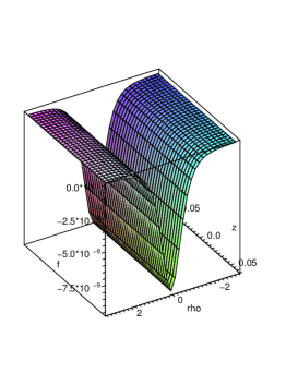
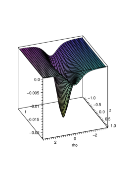
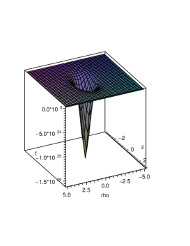
(a)	(b)	(c)

Figure 2: The harmonic function $-R_{11}^{6}/(2\pi^{2}{\ell_{p}}^{6}N)f(\rho,z)$ (where $f(\rho,z)$ is given by (B)) for (a) $L/R_{11}=50$, (b) $L/R_{11}=3$, and (c) $L/R_{11}=10^{-4}$.

Appendix C Radial expectation values

In order to compute the expectation value $\langle r\rangle$ (of the radial coordinate), the radial eigenfunctions must be normalized. Here, we normalize the modes following the prescription of ref. [39]. We briefly review their formalism (which is a simple generalization of the usual normalization of modes in four dimensional quantum field theory) before modifying it appropriately for our uses.

Consider a scalar field propagating in a $(d+1+k)$-dimensional spacetime with metric

$$ds^{2}(g)=f(y)\eta_{\mu\nu}dx^{\mu}dx^{\nu}+g_{\perp mn}dy^{m}dy^{n}$$

where $\mu,\nu=0,...d$, $m,n=1,...,k$. For a scalar field with the Lagrangian density

$$\mathcal{L}=\sqrt{-g}g^{ab}\partial_{a}\Phi\partial_{b}\Phi,$$ (140)

the canonical commutator is

$$\left[\Phi({\bf x},y),\dot{\Phi}({\bf x}^{\prime},y^{\prime})\right]=i\frac{f(y)}{\sqrt{-g}}\delta^{d}({\bf x}-{\bf x}^{\prime})\delta^{k}(y-y^{\prime}).$$

Specializing for the moment to the case $d=4$ and expanding the field as

$$\Phi(x,y)=\sum_{\alpha}\int\frac{D^{3}{\bf k}}{(2\pi)^{3}}\frac{1}{2k_{0}}\left(a_{\alpha}({\bf k})e^{ik\cdot x}\psi_{\alpha}(y)+h.c.\right)$$

with the oscillators covariantly normalized as $[a_{\alpha}({\bf k}),a_{\beta}^{\dagger}({\bf k}^{\prime})]=(2\pi)^{3}\delta^{(3)}({\bf k}-{\bf k^{\prime}})\delta_{\alpha\beta}$, the modes in $y$-space are then normalized according to

$$\int d^{k}y\frac{\sqrt{g}}{f}\psi_{\alpha}(y)\psi_{\beta}^{\ast}(y)=\delta_{\alpha\beta}.$$

For any one of the D$p$-D$k$ brane configurations, the Lagrangian density for the scalar fields $\chi$ corresponding to fluctuations of the D$k$-brane transverse to the D$p$-branes was (omitting multiplicative constants)

$$\mathcal{L}=e^{-\phi}\sqrt{-\det g_{ab}}f^{-1}g^{a}b\partial_{a}\chi\partial_{b}\chi$$ (141)

where $g_{ab}$ is the induced metric on the D$k$-brane. Comparing (140) and (141) suggests that for the scalar field confined to the D$k$-brane, the factor $\sqrt{-\det g_{ab}}$ should be replaced by $e^{-\phi}\sqrt{-\det g_{ab}}f^{-1}$. Thus, the canonical commutator should be

$$\left[\chi({\bf x},y),\dot{\chi}({\bf x}^{\prime},y^{\prime})\right]=i\frac{f(y)}{e^{-\phi}\sqrt{-\det g_{ab}}f^{-1}}\delta^{d}({\bf x}-{\bf x}^{\prime})\delta^{k}(y-y^{\prime})$$

and with $\chi$ expanded in terms of Fourier modes and spherical harmonics (as described in the text), the measure for the normalization for the radial functions $\phi(\varrho)$ should be

$$\mu(\varrho)=e^{-\phi}\sqrt{-\det g_{ab}}f^{-2}.$$ (142)

Hence, the radial expectation value of any function will be given by

$$\langle f(\varrho)\rangle=\frac{\int_{0}^{\infty}f(\varrho)\,\mu(\varrho)|\phi(\varrho)|^{2}d\varrho}{\int_{0}^{\infty}\mu(\varrho)|\phi(\varrho)|^{2}d\varrho}.$$ (143)

where the radial measure for any one of the D$p$-D$k$ brane systems is

$$\mu_{p,k}(\varrho)=\frac{\varrho^{1+\frac{k-p}{2}}}{(1+\varrho^{2})^{\frac{7-p}{2}}}.$$

Given the standard duality between energy and radius, i.e., $U=r/\alpha^{\prime}$, the radial profiles give the wave-function in energy — that is, $\mu(\varrho)|\phi(\varrho)|^{2}$ serves somewhat like a parton distribution function. The expectation value $\langle r\rangle$ gives a measure of the mean energy of the components of a given meson state. Using (143) and $\phi(\varrho)$ for the transverse scalar fluctuations of the probe brane, we computed $2\pi\langle U\rangle/m_{q}=\langle(1+\varrho^{2})^{1/2}\rangle$ for the D$p$-D$k$ systems. Note that for $p=3$, the calculations can be done analytically while for $p\neq 3$, the results are obtained numerically. Explicit results for the D2-D4 and D4-D6 configurations are displayed in Table 3. These are typical of the general case. Note that $\langle U\rangle$ increases when the radial quantum number is increased, but decreases with increasing $\ell_{2}$.

In [1], it was noted for the D3-D7 system that for large R-charge, $\ell\gg n$, the radial profiles were sharply peaked at $\varrho_{\rm peak}=1$. One can see that the same peaking arises for the mesons on other probe branes in the D3 background from the analytic solutions, e.g., , eqs. (119), (122) and (130). This radius corresponds to the radius of a null geodesic on the induced probe brane metric orbiting on the internal space at a constant value of $\varrho$. One expects a similar peaking for occurs for general $p$, for which the geodesic analysis yields $\varrho_{\rm peak}^{2}=2/(5-p)$. For the large R-charge limit, $\ell\gg n$, one can then infer $2\pi\langle U\rangle/m_{q}\simeq\sqrt{(7-p)/(5-p)}$.

References

- [1] M. Kruczenski, D. Mateos, R.C. Myers and D.J. Winters, “Meson spectroscopy in AdS/CFT with flavour,” JHEP 0307 (2003) 049 [arXiv:hep-th/0304032].
-
[2]
J.M. Maldacena, “The large N limit of superconformal
field theories and supergravity,” Adv. Theor. Math. Phys. 2 (1998) 231 [arXiv:hep-th/9711200];
-
[3]
S. S. Gubser, I. R. Klebanov and A. M. Polyakov, “Gauge theory correlators from non-critical string theory,” Phys. Lett. B 428 (1998) 105 [arXiv:hep-th/9802109];
E. Witten, “Anti-de Sitter space and holography,” Adv. Theor. Math. Phys. 2 (1998) 253 [arXiv:hep-th/9802150]. - [4] N. Itzhaki, J.M. Maldacena, J. Sonnenschein and S. Yankielowicz, “Supergravity and the large N limit of theories with sixteen supercharges,” Phys. Rev. D 58 (1998) 046004 [arXiv:hep-th/9802042].
- [5] O. Aharony, S.S. Gubser, J.M. Maldacena, H. Ooguri and Y. Oz, “Large N field theories, string theory and gravity,” Phys. Rept. 323 (2000) 183 [arXiv:hep-th/9905111].
- [6] A. Karch and E. Katz, “Adding flavor to AdS/CFT,” JHEP 0206 (2002) 043 [arXiv:hep-th/0205236].
- [7] M. Kruczenski, D. Mateos, R.C. Myers and D.J. Winters, “Towards a holographic dual of large- QCD,” JHEP 0405 (2004) 041 [arXiv:hep-th/0311270].
-
[8]
A. Fayyazuddin and M. Spalinski,
“Large N superconformal gauge theories and supergravity
orientifolds,” Nucl. Phys. B 535 (1998) 219
[arXiv:hep-th/9805096];
O. Aharony, A. Fayyazuddin and J.M. Maldacena, “The large N limit of N = 2,1 field theories from three-branes in F-theory,” JHEP 9807 (1998) 013 [arXiv:hep-th/9806159];
M. Grana and J. Polchinski, “Gauge / gravity duals with holomorphic dilaton,” Phys. Rev. D 65 (2002) 126005 [arXiv:hep-th/0106014];
M. Bertolini, P. Di Vecchia, M. Frau, A. Lerda and R. Marotta, “N = 2 gauge theories on systems of fractional D3/D7 branes,” Nucl. Phys. B 621 (2002) 157 [arXiv:hep-th/0107057];
M. Bertolini, P. Di Vecchia, G. Ferretti and R. Marotta, “Fractional branes and N = 1 gauge theories,” Nucl. Phys. B 630 (2002) 222 [arXiv:hep-th/0112187];
X.J. Wang and S. Hu,“Intersecting branes and adding flavors to the Maldacena-Nunez background,” JHEP 0309 (2003) 017 [arXiv:hep-th/0307218];
P. Ouyang, “Holomorphic D7-branes and flavored N = 1 gauge theories,” Nucl. Phys. B 699 (2004) 207 [arXiv:hep-th/0311084];
L.A. Pando Zayas, J. Sonnenschein and D. Vaman, “Regge trajectories revisited in the gauge / string correspondence,” Nucl. Phys. B 682 (2004) 3 [arXiv:hep-th/0311190];
E. Schreiber, “Excited mesons and quantization of string endpoints,” [arXiv:hep-th/0403226];
N.J. Evans and J.P. Shock, “Chiral dynamics from AdS space,” Phys. Rev. D 70 (2004) 046002 [arXiv:hep-th/0403279];
J.L.F. Barbon, C. Hoyos, D. Mateos and R.C. Myers,“The holographic life of the ,” JHEP 0410 (2004) 029 [arXiv:hep-th/0404260];
A. Armoni, “Witten-Veneziano from Green-Schwarz,” JHEP 0406 (2004) 019 [arXiv:hep-th/0404248];
K. Ghoroku and M. Yahiro, “Chiral symmetry breaking driven by dilaton,” Phys. Lett. B 604 (2004) 235 [arXiv:hep-th/0408040];
D. Arean, D.E. Crooks and A.V. Ramallo, “Supersymmetric probes on the conifold,” JHEP 0411 (2004) 035 [arXiv:hep-th/0408210];
M. Kruczenski, L.A.P. Zayas, J. Sonnenschein and D. Vaman, “Regge trajectories for mesons in the holographic dual of large-N(c) QCD,” JHEP 0506 (2005) 046 [arXiv:hep-th/0410035];
D. Bak and H. U. Yee, “Separation of spontaneous chiral symmetry breaking and confinement via AdS/CFT correspondence,” Phys. Rev. D 71 (2005) 046003 [arXiv:hep-th/0412170];
K. Ghoroku, T. Sakaguchi, N. Uekusa and M. Yahiro, “Flavor quark at high temperature from a holographic model,” Phys. Rev. D 71 (2005) 106002 [arXiv:hep-th/0502088];
N. Evans, J. Shock and T. Waterson, “D7 brane embeddings and chiral symmetry breaking,” JHEP 0503 (2005) 005 [arXiv:hep-th/0502091];
F. Bigazzi, R. Casero, A. L. Cotrone, E. Kiritsis and A. Paredes, “Non-critical holography and four-dimensional CFT’s with fundamentals,” JHEP 0510 (2005) 012 [arXiv:hep-th/0505140];
R. Apreda, J. Erdmenger and N. Evans, “Scalar effective potential for D7 brane probes which break chiral symmetry,” [arXiv:hep-th/0509219];
R. Casero, A. Paredes and J. Sonnenschein, “Fundamental matter, meson spectroscopy and non-critical string/gauge duality,” JHEP 0601 (2006) 127 [arXiv:hep-th/0510110];
K. Peeters, J. Sonnenschein and M. Zamaklar, “Holographic decays of large-spin mesons,” JHEP 0602 (2006) 009 [arXiv:hep-th/0511044];
A. L. Cotrone, L. Martucci and W. Troost,“String splitting and strong coupling meson decay,” Phys. Rev. Lett. 96 (2006) 141601 [arXiv:hep-th/0511045];
F. Canoura, J.D. Edelstein, L.A.P. Zayas, A.V. Ramallo and D. Vaman, “Supersymmetric branes on AdS(5) x Y**(p,q) and their field theory duals,” JHEP 0603 (2006) 101 [arXiv:hep-th/0512087];
R. Apreda, J. Erdmenger, N. Evans, J. Grosse and Z. Guralnik, “Instantons on D7 brane probes and AdS/CFT with flavour,” [arXiv:hep-th/0601130];
N. Evans and T. Waterson, “Improving the infra-red of holographic descriptions of QCD,” [arXiv:hep-ph/0603249]. -
[9]
T. Sakai and S. Sugimoto, “Low energy hadron physics in
holographic QCD,” Prog. Theor. Phys. 113 (2005) 843
[arXiv:hep-th/0412141];
T. Sakai and S. Sugimoto, “More on a holographic dual of QCD,” Prog. Theor. Phys. 114 (2006) 1083 [arXiv:hep-th/0507073]. -
[10]
A. Karch, E. Katz and N. Weiner, “Hadron masses and screening from
AdS Wilson loops,” Phys. Rev. Lett. 90 (2003) 091601
[arXiv:hep-th/0211107];
T. Sakai and J. Sonnenschein, “Probing flavored mesons of confining gauge theories by supergravity,” JHEP 0309 (2003) 047 [arXiv:hep-th/0305049];
J. Babington, J. Erdmenger, N.J. Evans, Z. Guralnik and I. Kirsch, “Chiral symmetry breaking and pions in non-supersymmetric gauge/gravity duals,” Phys. Rev. D 69, 066007 (2004) [arXiv:hep-th/0306018];
C. Nunez, A. Paredes and A.V. Ramallo, “Flavoring the gravity dual of N=1 Yang-Mills with probes,” JHEP 0312, 024 (2003) [arXiv:hep-th/0311201];
S. Kuperstein, “Meson spectroscopy from holomorphic probes on the warped deformed conifold,” JHEP 0503 (2005) 014 [arXiv:hep-th/0411097];
I. Brevik, K. Ghoroku and A. Nakamura, “Meson mass and confinement force driven by dilaton,” Int. J. Mod. Phys. D 15 (2006) 57 [arXiv:hep-th/0505057];
D. Arean, A. Paredes and A.V. Ramallo, “Adding flavor to the gravity dual of non-commutative gauge theories,” JHEP 0508 (2005) 017 [arXiv:hep-th/0505181];
T.S. Levi and P. Ouyang, “Mesons and flavor on the conifold,” [arXiv:hep-th/0506021];
M.J. Rodriguez and P. Talavera, “A 1+1 field theory spectrum from M theory,” [arXiv:hep-th/0508058];
J.P. Shock, “Canonical coordinates and meson spectra for scalar deformed N = 4 SYM from the AdS/CFT correspondence,” [arXiv:hep-th/0601025]. - [11] J. Erdmenger and I. Kirsch, “Mesons in gauge/gravity dual with large number of fundamental fields,” JHEP 0412 (2004) 025 [arXiv:hep-th/0408113].
- [12] D. Arean and A.V. Ramallo, “Open string modes at brane intersections,” [arXiv:hep-th/0602174].
- [13] N. Seiberg, “Why is the matrix model correct?,” Phys. Rev. Lett. 79 (1997) 3577 [arXiv:hep-th/9710009].
- [14] C.V. Johnson, D-Branes, Cambridge University Press (2003).
- [15] R.C. Myers, “Dielectric-branes,” JHEP 9912 (1999) 022 [arXiv:hep-th/9910053].
- [16] O. DeWolfe, D.Z. Freedman and H. Ooguri, “Holography and defect conformal field theories,” Phys. Rev. D 66 (2002) 025009 [arXiv:hep-th/0111135].
- [17] P. Pasti, D.P. Sorokin and M. Tonin, “Covariant action for a D = 11 five-brane with the chiral field,” Phys. Lett. B 398 (1997) 41 [arXiv:hep-th/9701037].
- [18] P.K. Townsend, “D-branes from M-branes,” Phys. Lett. B 373 (1996) 68 [arXiv:hep-th/9512062].
- [19] A.W. Peet and J. Polchinski, “UV/IR relations in AdS dynamics,” Phys. Rev. D 59 (1999) 065011 [arXiv:hep-th/9809022].
- [20] O. Pelc and R. Siebelink, “The D2-D6 system and a fibered AdS geometry,” Nucl. Phys. B 558 (1999) 127 [arXiv:hep-th/9902045].
- [21] G.T. Horowitz and J. Polchinski, “Gauge/gravity duality,” [arXiv:gr-qc/0602037].
- [22] E. Antonyan, J.A. Harvey, S. Jensen and D. Kutasov, “NJL and QCD from string theory,” [arXiv:hep-th/0604017].
-
[23]
O. Aharony, J. Sonnenschein and S. Yankielowicz, “A
holographic model of deconfinement and chiral symmetry
restoration,” [arXiv:hep-th/0604161];
A. Parnachev and D.A. Sahakyan, “Chiral Phase Transition from String Theory,” [arXiv:hep-th/0604173]. - [24] M. Kruczenski, R.C. Myers, S. Sugimoto and R.M. Thomson, in preparation/unpublished.
- [25] D. Mateos, R.C. Myers and R.M. Thomson, “Holographic Phase Transitions with Fundamental Matter,” in preparation.
-
[26]
T. Barnes, S. Godfrey and E.S. Swanson, “Higher charmonia,”
Phys. Rev. D 72 (2005) 054026
[arXiv:hep-ph/0505002];
S. Godfrey and N. Isgur, “Mesons In A Relativized Quark Model With Chromodynamics,” Phys. Rev. D 32 (1985) 189. - [27] S. Hong, S. Yoon and M.J. Strassler, “Quarkonium from the fifth dimension,” JHEP 0404 (2004) 046 [arXiv:hep-th/0312071].
- [28] O. Aharony, “A brief review of ’little string theories’,” Class. Quant. Grav. 17 (2000) 929 [arXiv:hep-th/9911147].
- [29] O. Aharony, A. Giveon and D. Kutasov, “LSZ in LST,” Nucl. Phys. B 691 (2004) 3 [arXiv:hep-th/0404016].
-
[30]
M. Rozali, “Matrix theory and U-duality in seven
dimensions,” Phys. Lett. B 400 (1997) 260
[arXiv:hep-th/9702136];
M. Berkooz, M. Rozali and N. Seiberg, “Matrix description of M theory on and ,” Phys. Lett. B 408 (1997) 105 [arXiv:hep-th/9704089]. - [31] S.A. Cherkis and A. Hashimoto, “Supergravity solution of intersecting branes and AdS/CFT with flavor,” JHEP 0211 (2002) 036 [arXiv:hep-th/0210105].
-
[32]
B.A. Burrington, J.T. Liu, L.A.P. Zayas and D. Vaman,
“Holographic duals of flavored N = 1 super Yang-Mills: Beyond the
probe approximation,” JHEP 0502 (2005) 022
[arXiv:hep-th/0406207];
I. Kirsch and D. Vaman, “The D3/D7 background and flavor dependence of Regge trajectories,” Phys. Rev. D 72 (2005) 026007 [arXiv:hep-th/0505164]. - [33] R. Casero, C. Nunez and A. Paredes, “Towards the string dual of N = 1 SQCD-like theories,” Phys. Rev. D 73 (2006) 086005 [arXiv:hep-th/0602027].
-
[34]
A. Paredes and P. Talavera, “Multiflavour excited mesons
from the fifth dimension,” Nucl. Phys. B 713 (2005) 438
[arXiv:hep-th/0412260];
J.L. Hovdebo and R.C. Myers, unpublished. - [35] J.L. Hovdebo, M. Kruczenski, D. Mateos, R.C. Myers and D.J. Winters, “Holographic mesons: Adding flavor to the AdS/CFT duality,” Int. J. Mod. Phys. A 20 (2005) 3428.
-
[36]
J.M. Maldacena, “Wilson loops in large N field
theories,” Phys. Rev. Lett. 80 (1998) 4859 [arXiv:hep-th/9803002];
S.J. Rey and J.T. Yee, “Macroscopic strings as heavy quarks in large N gauge theory and anti-de Sitter supergravity,” Eur. Phys. J. C 22 (2001) 379 [arXiv:hep-th/9803001];
A. Brandhuber, N. Itzhaki, J. Sonnenschein and S. Yankielowicz, “Wilson loops, confinement, and phase transitions in large N gauge theories from supergravity,” JHEP 9806 (1998) 001 [arXiv:hep-th/9803263]. - [37] H.W. Wyld, Mathematical Methods for Physics, Perseus Books (1976).
- [38] R.C. Myers, “Higher Dimensional Black Holes In Compactified Space-Times,” Phys. Rev. D 35 (1987) 455.
- [39] J. Polchinski and M.J. Strassler, “Hard scattering and gauge/string duality,” Phys. Rev. Lett. 88, 031601 (2002) [arXiv:hep-th/0109174].