SNUST 060402

UT-06-06

hep-th/0605013

Unitarity Meets Channel-Duality

for

Rolling/Decaying D-Branes

Yu Nakayama^a, Soo-Jong Rey^b, Yuji Sugawara^a

^a Department of Physics, University of Tokyo

7-3-1 Hongo, Bunkyo-ku, Tokyo 113-0033 JAPAN

^b School of Physics and Astronomy & BK-21 Physics Division

Seoul National University, Seoul 151-747 KOREA

abstract

Investigations for decay of unstable D-brane and rolling of accelerated D-brane dynamics have revealed that various proposed prescriptions give different result for spectral amplitudes and observables. Here, we study them with particular attention to unitarity and open-closed channel duality. From ab initio derivation in the open string channel, both in Euclidean and Lorentzian worldsheet approaches, we find heretofore overlooked contribution to the spectral amplitudes and obervables. The contribution is fortuitously absent for decay of unstable D-brane, but is present for rolling of accelerated D-brane. We finally show that the contribution is imperative for ensuring unitarity and optical theorem at each order in string loop expansion.

The shortest path between two truths in the real domain

passes through the complex domain. — J. Hadamard

1 Introduction

In Lorentz invariant quantum field theory, two of the most fundamental properties are locality and unitarity. The locality is necessary for the theory to obey causality. In turn, the microcausality, expressed in the commutativity of local operators at spacelike separations, leads to analyticity of scattering amplitudes and analytic continuation thereof. The unitarity is necessary for the theory to admit meaningful probabilistic interpretation. In turn, requiring unitarity to the scattering amplitudes, one obtains information concerning discontinuities about their branch points . In particular, Feynman’s $+i\varepsilon$ prescription on propagators together with Cutkovsky-Landau cutting rules provides a simple account for the causality and the unitarity. The Wick rotations and optical theorem are the simplest consequences of such [1].

In perturbative string theory, it was established that string scattering amplitudes are Lorentz invariant, unitary and local despite extended nature of string. Unlike quantum field theory, however, unitarity and locality are not manifest in the rules of perturbation theory. Instead, the unitarity was established only indirectly by showing equivalence between the covariant and the light-cone formulations of scattering amplitudes. Also, the locality was proven only by resorting to string field theory [2]. To date, establishing analyticity and analytic continuations of multi-loop scattering amplitudes have largely remained an outstanding unsolved problem in string theory. The issue is somewhat more involved than quantum field theory by the built-in channel duality between $s$- and $t$-channels, which exchanges the open and the closed string channels for string loop amplitudes.

In recent years, numerous works addressed string dynamics in a variety of time-dependent background. It includes timelike Liouville theory [3], strings in null orbifolds [4] or cosmological backgrounds [5], open string dynamics in electric field [6] or various time-dependent backgrounds [7], decay of unstable D-branes [8] and rolling of accelerated D-branes [9] in the NS5-brane backgrounds. Each of these investigations involved one way or another certain prescription of analyticity and analytic continuation of scattering amplitudes involving string states and D-branes. Those prescriptions were largely case-specific and often exploited analytic continuations of not only spacetime variables but also parameters defining the string worldsheet dynamics. Thus, it was far from transparent whether such prescriptions are mutually consistent and, after all, correct .

The purpose of this work is to bring out certain consistency checks of the prescription we proposed recently in the context of rolling D-branes in NS5-brane backgrounds [12, 13, 14] (see also [15, 16]), and compare critically with different prescriptions put forward by other works in this context [17] and the decay of unstable D-branes [18, 19, 20]. The central issue is whether analytic continuation can be prescribed in transition amplitudes of these processes in a way the optical theorem is manifest and right. Indeed, we shall show that certain prescriptions that arose from one context does not lead to self-consistent results when applied to other contexts. We shall also show that some other prescriptions adopted in the literatures are inconsistent and incorrect.

As said, we shall address the questions primarily in the context of rolling of accelerated D-brane in NS5-brane background [9] and of decay of unstable D-brane (either in flat space [18], in linear dilaton background [19] or in two-dimensional string theory [20]). Both situations involve conversion of the energy stored in the D-brane to elementary string states. In the process, formally, the optical theorem facilitates to extract emission spectra of the decaying or rolling D-brane from forward scattering amplitude of the D-brane. In string perturbation theory, the leading order contribution comes from the cylinder amplitude. Typically, the amplitude is ill-defined and requires careful prescription.

In the previous works [12, 13, 14], we studied rolling dynamics of accelerated D-brane in NS5-brane background and two-dimensional black hole geometry, described by ${\cal N}=2$ superconformal SL$(2,\mathbb{R})/$U(1) model. We extracted cylinder amplitude in Lorentzian worldsheet and Lorentzian spacetime, respectively, via $+i\varepsilon$ prescriptions. The prescriptions were devised to render the modular integral (Schwinger-Feynman integral) of the amplitude well-defined and analytic. In particular, after integrating over the worldsheet modulus, the amplitude expressed in the closed string channel develops an imaginary part corresponding to total emission of on-shell closed string states, thus ensuring the optical theorem to hold. The total radiation number was given in the closed string channel by [12, 13, 14]

$$\overline{\cal N}=\sum_{M}\sqrt{\rho^{(c)}(M)}\int_{0}^{\infty}{{\rm d}p\over 2\omega}{\sinh{2\pi\over Q}\sqrt{\frac{\alpha^{\prime}}{2}}p\over\left[\cosh{2\pi\over Q}\sqrt{\frac{\alpha^{\prime}}{2}}\omega+\cosh{2\pi\over Q}\sqrt{\frac{\alpha^{\prime}}{2}}p\right]\sinh\pi Q\sqrt{\frac{\alpha^{\prime}}{2}}p}~{},$$

where $\rho^{(c)}(M)$ is density of states and $\omega\equiv\sqrt{p^{2}+M^{2}}$ is on-shell energy of the left-right symmetric closed string states.

Utilizing the open-closed channel duality, spectral amplitudes and observables ought to be re-expressible in the open string channel via (generalized) Fourier transform. The procedure is not always straightforward and, as we will see in this work, requires careful treatment of various Fourier transformations involved. In this work, we undertake ab initio analysis of the spectral amplitudes and observables and find that the Fourier transformations are generically not convergent. They require suitable analytic continuations and we propose a specific prescription for how to do so. With the prescription, we find that both spectral amplitudes and observables contain new contribution from the analytic continuation in addition to naive contribution. So, for the total emission number $\overline{\cal N}$ and the cylinder amplitude $Z_{\rm cylinder}$, the results take schematically the form:

$$\overline{\cal N} = \int_{0}^{\infty}{{\rm d}t_{o}\over t_{o}}\Big{(}F_{\rm naive}(t_{o})+F_{\rm pole}(t_{o})\Big{)}$$

$$Z_{\rm cylinder} = Z_{\rm naive}+Z_{\rm pole}~{},$$ (1.1)

viz. sum of the naive part and the new contribution part. The naive part is the result obtained based on a tacit assumption that the Fourier transforms between open and closed string channels are always convergent.

Moveover, the analytic continuations we propose are not only mathematically correct but also physically justified: the naive part do not obey the optical theorem, whereas sum of the naive and the new parts do so. Stated differently, consistency between the open-closed channel duality and the unitarity in string perturbation theory require the Fourier transform to be defined via the analytic continuations proposed in this work. We believe the results in this work clarify much of confusion in previous works concerning spectral amplitudes and observables for the decay of unstable D-brane and the rolling of accelerated D-brane. In particular, it shows that the prescription of [19] in the context of the decay of unstable D-brane yielded fortuitously correct result in that the extra pole contribution turns out absent and that the prescription of [19] cannot be taken over to other contexts such as the rolling of accelerated D-brane as was done, for example, in [17].

This paper is organized as follows. In section 2, we first recapitulate computation of spectral amplitudes and observables for the decay of unstable D-brane in open and closed string channels, in flat spacetime, in linear dilaton background, and in two-dimensional string theory background. We demonstrate that the Fourier transform between open string and closed string channels is fortuitously convergent. Consequently, only the naive contributions being present, the unitarity and the channel duality are obeyed trivially. In section 3, we study the same for the rolling of accelerated D-brane, where the acceleration is caused by extremal or non-extremal NS5-brane background. Here, we find that the extra pole contribution shows up. Consequently, the optical theorem is seen to follow only if this extra contribution is taken account of. In section 4, we highlight important steps in the proposed analytic continuation of the Fourier transform, and tie up loose ends of various confusion scattered in the previous works [17, 19].

2 Decay of Unstable D-brane

For completeness and for detailed comparison with rolling D-brane case, we shall first compute closed string emission out of decaying D-brane in linear dilaton background following closely the method employed in the appendix of [19]. The dilaton gradient is set by:

$$\Phi={1\over\sqrt{\alpha^{\prime}}}(Q\,X^{0}+{\bf V}\cdot{\bf X}),\qquad\mbox{where}\qquad Q\equiv\beta-{1\over\beta}~{}\qquad(\beta\geq 1)~{}.$$ (2.1)

This puts the critical dimension $D$ for the bosonic string theory to be

$$26=D-6Q^{2}+6{\bf V}^{2},\qquad\mbox{so}\qquad c_{\rm eff}=6Q_{\beta}^{2}-6{\bf V}^{2}~{},$$ (2.2)

where $Q_{\beta}\equiv(\beta+1/\beta)$. The effective central charge $c_{\rm eff}$ sets the growth of density of closed string states [21]:

$$\rho^{(c)}(M)\sim e^{4\pi\sqrt{\frac{c_{\mbox{\scriptsize eff}}}{24}\alpha^{\prime}M^{2}}}$$ (2.3)

up to subleading pre-exponential factor of $M$. It grows slower than the density of states for flat spacetime (obtainable by setting $Q={\bf V}=0$).

2.1 closed string emission

Consider the decay of an unstable D-brane in linear dilaton background. The radiative transition of a D$p$-brane to a single closed string state of mass $M$ (set by the integer-valued oscillator level $N=\widetilde{N}$), whose on-shell energy-momentum $(\omega,{\bf k})$ is given by

$$\Big{(}\omega_{E}-{iQ\over\sqrt{\alpha^{\prime}}}\Big{)}^{2}-\Big{(}{\bf k}_{E}+{i{\bf V}\over\sqrt{\alpha^{\prime}}}\Big{)}^{2}=(\omega^{2}-{\bf k}^{2})=M^{2}\quad\mbox{where}\quad\frac{1}{4}\,\alpha^{\prime}M^{2}=N-{c_{\rm eff}\over 24},$$ (2.4)

where $(\omega_{E},{\bf k}_{E})$ and $(\omega,{\bf k})$ are energy-momenta in the Einstein and the string frame, respectively. In string loop perturbation theory, the transition amplitude is computed by the disk one-point function $\langle\exp((-i\omega+\frac{Q}{\sqrt{\alpha^{\prime}}})X^{0})\,\exp((i{\bf k}+\frac{{\bf V}}{\sqrt{\alpha^{\prime}}})\cdot{\bf X})\rangle_{\mbox{\scriptsize disk}}$ with the D$p$-brane boundary condition, where the vertex operator is separated into temporal and spatial parts as indicated. The two parts are factorized in the gauge that no oscillator in temporal direction is allowed. Consequently, the transition probability ${\cal P}(\omega)$ of the radiative process is governed entirely by the temporal part (see (3.29) in [19]):

$${\cal P}(\omega)=\Big{|}\left\langle e^{(-i\omega+\frac{Q}{\sqrt{\alpha^{\prime}}})X^{0}}e^{(i{\bf k}+\frac{{\bf V}}{\sqrt{\alpha^{\prime}}})\cdot{\bf X}}\right\rangle_{\mbox{\scriptsize disk}}\Big{|}^{2} = \Big{|}{1\over\beta}\Gamma(1+i\omega\sqrt{\alpha^{\prime}}\beta)\Gamma(-i\omega\sqrt{\alpha^{\prime}}/\beta)\Big{|}^{2}$$ (2.5)

$$= {\pi^{2}/\beta^{2}\over\sinh(\pi\omega\sqrt{\alpha^{\prime}}\beta)\sinh(\pi\omega\sqrt{\alpha^{\prime}}/\beta)}~{}.$$

Then, at leading order in string perturbation theory, the total number of emitted closed strings from the decay of a D$p$-brane ($p\geq 1$) extended along ${\bf V}$-direction is computed as

$$\overline{\cal N}=N_{p}^{2}V_{p}\sum_{M}\sqrt{\rho^{(c)}(M)}\int_{-\infty}^{\infty}\!{{\rm d}^{D-1-p}{\bf k}\over(2\pi)^{D-1-p}}\,{1\over 2\omega}{\cal P}(\omega)~{},$$ (2.6)

where the overall coefficient abbreviates $N_{p}=\pi^{\frac{D-4}{4}}(2\pi)^{\frac{D-2}{4}-p}$ and $V_{p}$ is the D$p$-brane volume. In (2.1), the sum is over all final closed string states of mass $M$ and of oscillator excitations symmetric between left- and right-moving sectors. Such oscillator excitations are equivalent in combinatorics to open string excitation, so the density of the final states is given by square-root of (2.3).

Attributed to the Hagedorn growth of the density of states $\rho^{(c)}(M)$, the total emission number $\overline{\cal N}$ in (2.1) (or higher spectral moment) is ultraviolet convergent so long as linear dilaton has a nonzero spatial component, ${\bf V}\neq 0$, first observed in [19]. Notice also that temporal component of the linear dilaton does not alter the ultraviolet behavior. This is most readily seen for small ${\bf V}$ by expanding the density of states. To study anatomy of the ultraviolet behavior, we shall now perform Fourier transformation and re-express $\overline{\cal N}$ in the open string channel.

2.2 open string channel viewpoint

Physical observables such as $\overline{\cal N}$ ought to be well-defined under the Fourier transform from the closed string channel to the open string one because

1. We start with defining expression of $\overline{\cal N}$, consistent with the optical theorem in the closed string channel.

2. The expression is closed in the Euclidean signature. Hence we are free from any subtlety that may arise from analytic continuations between Euclidean and Lorentzian signature of the spacetime.

As in [19], expand the transition probability ${\cal P}(\omega)$ in convergent power series, whose terms are interpretable as D-instantons arrayed along imaginary time coordinate:

$${\cal P}(\omega)={4\pi^{2}\over\beta^{2}}\sum_{n,m=0}^{\infty}e^{-2\pi\alpha^{\prime}\omega W(m,n)}$$ (2.7)

where the location of the D-instantons is denoted as

$$\alpha^{\prime}W(m,n)=\sqrt{\alpha^{\prime}}\Big{[}\Big{(}n+{1\over 2}\Big{)}\beta+\Big{(}m+{1\over 2}\Big{)}{1\over\beta}\Big{]}\geq\sqrt{\alpha^{\prime}}~{}.$$ (2.8)

So, we take

$$\overline{\cal N}=\Big{(}{2\pi N_{p}\over\beta}\Big{)}^{2}V_{p}\sum_{M}\int_{-\infty}^{\infty}{{\rm d}^{D-1-p}{\bf k}\over(2\pi)^{D-1-p}}\sum_{m,n=0}^{\infty}{1\over 2\omega}e^{-2\pi\alpha^{\prime}\omega W(m,n)}$$ (2.9)

and rewrite each D-instanton contribution parametrically via the closed string channel modulus $t_{c}$ as

$${1\over 2\omega}e^{-2\pi\alpha^{\prime}\omega W(m,n)} = \frac{\pi\alpha^{\prime}}{2}\int_{-\infty}^{\infty}{{\rm d}k_{0}\over 2\pi}\int_{0}^{\infty}{\rm d}{t_{c}}\,e^{-2\pi t_{c}\cdot\frac{1}{4}\alpha^{\prime}(k_{0}^{2}+{\bf k}^{2}+M^{2})}e^{2\pi i\alpha^{\prime}k_{0}W(m,n)}.$$ (2.10)

This gives

$$\overline{\cal N}\!\!\! = \!\!\!\!\Big{(}{2\pi N_{p}\over\beta}\Big{)}^{2}V_{p}\frac{\pi\alpha^{\prime}}{2}\sum_{m,n=0}^{\infty}\int_{0}^{\infty}{\rm d}{t_{c}}\int_{-\infty}^{\infty}{{\rm d}k_{0}\over 2\pi}\int_{-\infty}^{\infty}{{\rm d}^{D-1-p}{\bf k}\over(2\pi)^{D-1-p}}\,e^{-2\pi t_{c}\cdot\frac{1}{4}\alpha^{\prime}(k_{0}^{2}+{\bf k}^{2})}e^{2\pi i\alpha^{\prime}k_{0}W(m,n)}$$ (2.11)

$$\hskip 105.2751pt\times\sum_{M}\sqrt{\rho^{(c)}(M)}e^{-2\pi t_{c}\cdot\frac{1}{4}\alpha^{\prime}M^{2}}.$$

Here, we exchanged order of summations and integrations, and first performed integrals over off-shell momenta $(k_{0},{\bf k})$ and sum over mass level $M$. The sum over $M$ yields modular covariant partition function $Z^{(c)}(q_{c})$ in terms of the Dedekind eta function:

$$Z^{(c)}(q_{c}) \equiv \sum_{M}\sqrt{\rho^{(c)}(M)}\,\,q_{c}^{\frac{1}{4}\alpha^{\prime}M^{2}}\qquad\mbox{where}\qquad q_{c}\equiv e^{-2\pi t_{c}}$$ (2.12)

$$= \eta^{-(D-2)}(q_{c})~{}.$$

Integrations over the $(D-p)$-dimensional momenta $(k_{0},{\bf k})$ yield $(2\pi^{4}\alpha^{\prime}t_{c})^{-(D-p)/2}$ times Gaussian damping factor $e^{-2\pi\alpha^{\prime}W^{2}(m,n)/t_{c}}$. We now perform modular transformation to the open string channel $t_{c}=1/t_{o}$, where $t_{o}$ is modulus of the open string channel and $q_{o}\equiv e^{-2\pi t_{o}}$. Putting all these together, we finally have

$$\overline{\cal N}=C_{p}\,V_{p}\sum_{m,n=0}^{\infty}\int_{0}^{\infty}{{\rm d}t_{o}\over t_{o}}t_{o}^{-p/2}\,e^{-2\pi t_{o}\alpha^{\prime}W^{2}(m,n)}\,\eta^{-(D-2)}(q_{o}),$$ (2.13)

with $C_{p}=\Big{(}{2\pi N_{p}\over\beta}\Big{)}^{2}\frac{\pi\alpha^{\prime}}{2}(2\alpha^{\prime}\pi^{4})^{-\frac{D-p}{2}}$, reproducing the result reported in [19]. As it stands, the final expression (2.13) is at odd to the intuition based on, for example, the Schwinger pair production in (time-dependent) electric field, since the integral over the open string modulus $t_{o}$ is still intact. If the total emission number is interpretable as arising from on-shell two-particle branch cut in the open string channel, the modulus integral ought to be absent! Therefore, To understand underlying physics better, we shall now compute the cylinder amplitude directly and then extract the imaginary part via the optical theorem.

2.3 Lorentzian cylinder amplitude

Unitarity and optical theorem thereof, combined with the open-closed string channel duality, should enable us to extract the emission number $\overline{\cal N}$ of closed strings from decaying D$p$-brane as the imaginary part of the cylinder amplitude. In the closed string channel diagram, the computation reduces to (2.1), as in quantum field theory. It is, however, somewhat nontrivial to evaluate the imaginary part of the cylinder amplitude directly from the open string channel. Here we present the ab initio derivation, refining that in the text of [19], by starting with manifestly well-defined Lorentzian cylinder amplitude.

We begin with the cylinder amplitude in the closed string channel in which both the worldsheet and the target spacetime signatures are taken Lorentzian. Omitting overall numerical factors for the moment, the amplitude is given by

$$Z_{\rm cylinder}=i\pi\alpha^{\prime}V_{p}\int_{s_{c}^{\rm IR}}^{s_{c}^{\rm UV}}{\rm d}s_{c}\int_{-\infty}^{\infty}\frac{{\rm d}\omega_{L}}{2\pi}\,\frac{\pi^{2}/\beta^{2}\cdot q_{c}^{-(1-i\hat{\epsilon})^{2}\frac{1}{4}\alpha^{\prime}\omega_{L}^{2}}}{\sinh(\pi\beta\omega_{L}\sqrt{\alpha^{\prime}})\sinh(\pi\omega_{L}\sqrt{\alpha^{\prime}}/\beta)}\,Z_{{\cal M}}^{(c)}(q_{c})\ ,$$ (2.14)

where $q_{c}=e^{2\pi i\tau_{c}}$ with $\tau_{c}=s_{c}+i\epsilon$, and $Z_{{\cal M}}(q_{c})$ represents the contribution from the closed string zero-modes and oscillator parts . The Lorentzian worldsheet is regularized by $i\epsilon$ prescription, while the Lorentzian spacetime is regularized by $-i\hat{\epsilon}$-prescription. $s_{c}^{\rm{UV}}$ ($s_{c}^{{\rm IR}}$) is an ultraviolet (infrared) regulator of the closed string channel modulus. With these prescriptions, the integral over $\omega_{L}$ is convergent so long as $2\hat{\epsilon}s_{c}^{\rm UV}>\epsilon>0$ is retained.

Defining the open string modular parameter as $q_{o}=e^{-2\pi i\tau_{o}}$ where $\tau_{o}=s_{o}-i\epsilon$ with $s_{o}=1/s_{c}$, one can rewrite (2.14) in terms of open string channel energy $\omega_{L}^{\prime}$ as

$$Z_{\rm cylinder} = V_{p}\int_{s_{o}^{\rm UV}}^{s_{o}^{\rm IR}}{{\rm d}s_{o}}\int_{-\infty}^{\infty}{\rm d}\omega^{\prime}_{L}\left(i\pi\alpha^{\prime}\int_{-\infty}^{\infty}{\rm d}\omega_{L}\frac{\cos(\pi\alpha^{\prime}\omega_{L}\omega^{\prime}_{L})}{\sinh(\pi\beta\omega_{L}\sqrt{\alpha^{\prime}})\sinh(\pi\omega_{L}\sqrt{\alpha^{\prime}}/\beta)}\right)$$ (2.15)

$$\hskip 113.81102pt\times\,q_{o}^{-(1+i\hat{\epsilon}^{\prime})^{2}\frac{1}{4}\alpha^{\prime}{\omega_{L}^{\prime}}^{2}}Z_{{\cal M}}^{(o)}(q_{o})\,,$$

where $s^{\rm IR}_{o}\equiv 1/s^{\rm UV}_{c}$, $s^{\rm UV}_{o}\equiv 1/s^{\rm IR}_{c}$ are the cut-off’s in the open string modulus. As opposed to the closed string channel, we have to adopt the $+i\hat{\epsilon}^{\prime}$-prescription for the Lorentzian space-time, and the above integral is well-defined as long as $2\hat{\epsilon}^{\prime}s^{\rm UV}_{o}>\epsilon$. The expression in the large parenthesis yields the open string density of states, $\rho^{(o)}(\omega^{\prime}_{L})$. It is infrared divergent at $\omega_{L}=0$. To regularize it, we subtract minimally the double pole  so that

$$\rho^{(o)}(\omega^{\prime}_{L})_{\mathrm{reg}} = i\pi\alpha^{\prime}\int_{-\infty}^{\infty}{\rm d}\omega_{L}\left(\frac{\cos(\pi\alpha^{\prime}\omega_{L}\omega^{\prime}_{L})}{\sinh(\pi\beta\omega_{L}\sqrt{\alpha^{\prime}})\sinh(\pi\omega_{L}\sqrt{\alpha^{\prime}}/\beta)}-\frac{1}{\pi^{2}\alpha^{\prime}\omega_{L}^{2}}\right)$$ (2.16)

$$= -{2}\partial_{\omega^{\prime}_{L}}\log S_{\beta}\left({Q}_{\beta}+i\sqrt{\alpha^{\prime}}\omega^{\prime}_{L}\right)\ ,$$ (2.17)

where the ‘$q$-Gamma function’ $S_{\beta}(x)$ is defined by 

$$-\partial_{x}\log S_{\beta}(x)=\int_{-\infty}^{\infty}{\rm d}t\left(\frac{\cosh((x-Q_{\beta})t)}{2\sinh(\beta t)\sinh(t/\beta)}-\frac{1}{2t^{2}}\right)\$$ (2.18)

for $\mathrm{Re}(x)<2Q_{\beta}$ and analytically continued to the whole complex plane . See, for example, [22, 23].

Now we perform the Wick-rotation both in the target space and on the worldsheet. First, Wick rotate the open string channel energy as $\omega^{\prime}_{L}\,\rightarrow\,e^{i(\frac{\pi}{2}-0)}\omega^{\prime}_{L}$ and set $\omega^{\prime}_{L}=i\omega^{\prime}$ $(\omega^{\prime}\in\mathbb{R})$. Then, we can safely Wick rotate the worldsheet Schwinger parameter as $s_{o}\,\rightarrow\,-it_{o}$ ($t>0$). Notice that we will need to perform the Euclidean rotation in opposite direction for the closed and the open string channels due to the difference of the $i\epsilon$-prescription. There is no obstruction in such contour deformation because $\partial_{x}\log S_{\beta}(x)$ has poles only on the real axis. We will see that this is specific to the decaying D-brane situation and do not hold generally. In fact, in section 3 dealing with the rolling D-branes, we shall show that there exist extra contributions from crossing poles in the course of the contour rotation and that their contributions are essential for maintaining the unitarity. After Wick rotating the worldsheet, the cylinder amplitude in the open string sector is given by

$$Z_{\rm cylinder}=-2V_{p}\int_{0}^{\infty}{\rm d}t_{o}\int_{(1-i0)\mathbb{R}}{\rm d}\omega^{\prime}\partial_{\omega^{\prime}}\log S_{\beta}\left({Q_{\beta}}-\sqrt{\alpha^{\prime}}\omega^{\prime}\right)q_{o}^{\frac{1}{4}\alpha^{\prime}{\omega^{\prime}}^{2}}Z_{M}^{(o)}(q_{o})\ .$$ (2.19)

Imaginary part of the partition function comes from the simple poles of the $q$-Gamma function $S_{\beta}\left(Q_{\beta}-\sqrt{\alpha^{\prime}}\omega^{\prime}\right)$ at $\frac{1}{2}\omega^{\prime}=W(m,n)$ for $n,m\in\mathbb{Z}_{\geq 0}$ and simple zeros for $n,m\in\mathbb{Z}_{<0}$. Therefore, collecting imaginary parts from the contour integration over $\omega^{\prime}$ and applying the optical theorem, we finally obtain

$$\overline{\cal N}=\mathrm{Im}\,Z_{\rm cylinder}=C_{p}\,V_{p}\sum_{n,m=0}^{\infty}\int_{0}^{\infty}{{\rm d}t_{o}\over t_{o}}t_{o}^{-\frac{p}{2}}\,e^{-2\pi t_{o}\alpha^{\prime}W^{2}(m,n)}\,\eta^{-(D-2)}(q_{o})\ ,$$ (2.20)

where we have evaluated the free oscillator part explicitly and reinstated overall numerical factors. This is in perfect agreement with (2.1), and it may be interpreted as a nontrivial check of unitarity and open-closed duality in the Lorentzian signature.

2.4 D-brane decay in two-dimensional string theory

In a similar method, one can compute the spectral observables from the D-brane decay in two-dimensional string theory. The boundary state for the unstable D-brane in two-dimension is given by the ZZ-brane boundary state [24]:

$$\langle e^{(ik+2/\sqrt{\alpha^{\prime}})\phi}\rangle_{\mbox{\scriptsize disk}}=\mu^{-\frac{i}{2}\sqrt{\alpha^{\prime}}k}\frac{2\sqrt{\pi}}{\Gamma(1-ik\sqrt{\alpha^{\prime}})\Gamma(ik\sqrt{\alpha^{\prime}})}\ .$$ (2.21)

Combining it with the rolling tachyon boundary states, the total emission number of closed string is given by

$$\overline{\cal N}=N_{o}^{2}\int^{\infty}_{0}{\rm d}k\int^{\infty}_{0}\frac{{\rm d}\omega}{2\omega}{\cal P}(\omega,k)\delta(\omega-k)\ ,$$ (2.22)

where the on-shell condition $\omega=k$ is imposed, and the transition probability is

$${\cal P}(\omega,k)=\left|\langle e^{-i\omega X^{0}}e^{(ik+2/\sqrt{\alpha^{\prime}})\phi}\rangle_{\mbox{\scriptsize disk}}\right|^{2}=\frac{\sinh^{2}(\pi k\sqrt{\alpha^{\prime}})}{\sinh^{2}(\pi\omega\sqrt{\alpha^{\prime}})}\ .$$ (2.23)

We see that, after performing the $k$-integration, the resultant total emission number is ultraviolet divergent.

To express $\overline{\cal N}$ in open string channel, we repeat the analysis of section 2.2 and expand the transition probability in arrays of imaginary D-instantons. The result is

$$\overline{\cal N} = N_{o}^{2}\sum_{m,n=0}^{\infty}\int_{0}^{\infty}{\rm d}k\int_{0}^{\infty}{\rm d}t_{c}\int_{-\infty}^{\infty}\frac{{\rm d}k_{0}}{2\pi}e^{-2\pi t_{c}\cdot\frac{1}{4}\alpha^{\prime}(k_{0}^{2}+k^{2})}e^{2\pi i\alpha^{\prime}k_{0}W(m,n)}\sinh^{2}(\pi k\sqrt{\alpha^{\prime}})\Big{|}_{\beta\rightarrow 1}$$ (2.24)

$$= N_{o}^{2}\sum_{m,n=0}^{\infty}\int_{0}^{\infty}\frac{{\rm d}t_{o}}{t_{o}}\Big{(}{1\over q_{o}}-1\Big{)}q_{o}^{\alpha^{\prime}W^{2}(m,n)}\Big{|}_{\beta\rightarrow 1}\ ,$$ (2.25)

where we have reinstated $W(m,n)$ for the purpose of regularization . The expressoin exhibits ultraviolet divergence as $t_{o}\to\infty$.

On the other hand, it is possible to obtain the same radiation rate from the direct evaluation of the imaginary part of the Lorentzian cylinder amplitude in the open-string channel as was done in section 2-3:

$$Z_{\rm cylinder}=iN_{o}^{2}\int_{0}^{\infty}{\rm d}s_{c}\int_{-\infty}^{\infty}\frac{{\rm d}\omega_{L}}{2\pi}\int_{0}^{\infty}\frac{{\rm d}k}{2\pi}\,\frac{\sinh(\pi\sqrt{\alpha^{\prime}}k)^{2}}{\sinh(\pi\sqrt{\alpha^{\prime}}\omega_{L})^{2}}\,q_{c}^{\frac{1}{4}\alpha^{\prime}(-\omega^{2}_{L}+k^{2})}\ .$$ (2.26)

After rewriting the open string density by the $q$-Gamma function as in section 2.3, we obtain open string channel expression of the partition function. We then find the imaginary part from the poles located at $\frac{1}{2}\omega^{\prime}=W(m,n)$, and reproduce (2.25). This confirms that the partition function is manifestly unitary, obeying the optical theorem. Here again, the regularization $\beta\to 1$ is implicit.

3 Rolling of Accelerated D-brane

Consider next rolling dynamics of accelerated D-brane. We first recapitulate rolling D-brane dynamics in the fivebrane background. For details, we refer the readers to [9, 12, 14]. The fermionic string background of interest is described by the exact conformal field theory:

$$\mathbb{R}_{t}\times\mathbb{R}_{\phi}\times{\cal M}\qquad\mbox{or}\qquad{\mbox{SL}(2)_{k}\over\mbox{U}(1)}\times{\cal M}\ ,$$ (3.1)

where $\mathbb{R}_{t}$ is the timelike free theory, $\mathbb{R}_{\phi}$ is the spacelike linear dilaton with slope $Q\equiv\sqrt{2/k}$, and ${\cal M}$ is a unitary rational conformal field theory describing the transverse geometry. The conformality condition relates the dilaton slope $Q$  to the central charge of ${\cal M}$:

$$c_{{\cal M}}+(3+3Q^{2})=15~{}.$$ (3.2)

We shall focus on the region $Q\leq\sqrt{2}$ viz. $k\geq 1$ for the moment, which corresponds to the ‘black-hole phase’ of the super-coset SL(2)_k/U(1) conformal field theory [25]. In the background of fivebranes, $k=1,2,\cdots$ counts the total number of fivebranes [26, 27].

Notice that the effective central charge of the background (3.1) is equal $c_{{\cal M}}$;

$$c_{\mbox{\scriptsize eff}}\equiv 12-24\cdot\frac{Q^{2}}{8}=12\Big{(}1-{1\over 4}Q^{2}\Big{)}=c_{{\cal M}}~{}.$$ (3.3)

Notice also that, from Cardy’s formula, the density of closed string state grows at ultraviolet asymptotically as

$$\rho^{(c)}(M)\sim e^{4\pi\sqrt{\frac{c_{\mbox{\scriptsize eff}}}{12}\cdot\frac{1}{2}\alpha^{\prime}M^{2}}}=e^{4\pi\sqrt{\left(1-\frac{1}{4}Q^{2}\right)\cdot\frac{1}{2}\alpha^{\prime}M^{2}}}$$ (3.4)

up to pre-exponential factors of $M$.

3.1 closed string emission

Consider a D0-brane placed initially in the background of (3.1). Subsequently, the D0-brane rolls toward the five-branes and forms a non-threshold bound-state. The emission number $\overline{\cal N}$ of the process is determined by the boundary wave function $\Psi(p,\omega)$ of the rolling D0-brane and was computed in [12, 15, 13] for the extremal NS5-branes. Explicitly, for the NS-sector,

$$\overline{\cal N}=N^{2}_{\rm NS}\sum_{M}\sqrt{\rho^{(c)}(M)}\int_{0}^{\infty}{{\rm d}p\over 2\pi}\,\frac{1}{2\omega}{\cal P}(p,\omega)~{},$$ (3.5)

where $N_{\rm NS}$ is an appropriate numerical factor normalizing the boundary states, $\omega=\sqrt{p^{2}+M^{2}}$ is the on-shell energy of the emitted closed string, and

$${\cal P}(p,\omega)\equiv\left|\Psi(p,\omega)\right|^{2}=\frac{\sinh\frac{2\pi}{Q}\sqrt{\frac{\alpha^{\prime}}{2}}p}{\left(\cosh\frac{2\pi}{Q}\sqrt{\frac{\alpha^{\prime}}{2}}p+\cosh\frac{2\pi}{Q}\sqrt{\frac{\alpha^{\prime}}{2}}\omega\right)\sinh\pi Q\sqrt{\frac{\alpha^{\prime}}{2}}p}~{}$$ (3.6)

is the transition probability. Essentially the same formula is also applicable to the ‘incoming radiation’ of rolling D-brane in the non-extremal NS5-brane background [14]. Notice that ${\cal P}(p,\omega)$ is a function of both $\omega$ and $p$, whereas it depended only on $\omega$ for the decaying D-branes considered in the previous section. This is because the unstable D-brane stays at rest during the decay process, while here the accelerated D-brane rolls along the direction $\mathbb{R}_{\phi}$.

In [12, 13, 14], the total emission number $\overline{\cal N}$ was computed in the closed string channel via the optical theorem $\overline{\cal N}=\mbox{Im}\,Z_{\mbox{\scriptsize cylinder}}$, where $Z_{\mbox{\scriptsize cylinder}}$ is the cylinder amplitude with rolling D-branes and the imaginary part arose from on-shell closed string states.

3.2 open string channel viewpoint

What is the nature of the ultraviolet behavior of the emission number $\overline{\cal N}$ and how is it compared to the decay of rolling D-brane? To answer these, we shall now recast (3.5) in the open string channel, following technical procedures considered in the previous section and appendix of [19].

We begin with expanding the transition probability ${\cal P}(p,\omega)$ of the D0-brane (3.6) in power series of contribution of imaginary branes:

$${\cal P}(p,\omega)=\sum_{n=1}^{\infty}a_{n}(p)e^{-2\pi n\frac{\omega}{Q}\sqrt{\frac{\alpha^{\prime}}{2}}}~{},$$ (3.7)

$$a_{n}(p)=2(-1)^{n+1}\frac{\sinh\left(\frac{2\pi n}{Q}\sqrt{\frac{\alpha^{\prime}}{2}}p\right)}{\sinh(\pi Q\sqrt{\frac{\alpha^{\prime}}{2}}p)}~{}.$$ (3.8)

As before, we parametrically rewrite (3.5) as

$$\overline{\cal N} = N_{\rm NS}^{2}\sum_{M}\sqrt{\rho^{(c)}(M)}$$ (3.9)

$$\times \int_{0}^{\infty}{{\rm d}p\over 2\pi}\sum_{n=1}^{\infty}\int_{-\infty}^{\infty}{{\rm d}k_{0}\over 2\pi}\,\int_{0}^{\infty}\frac{\alpha^{\prime}}{2}{\rm d}t_{c}\,a_{n}(p)e^{\frac{2\pi in}{Q}\sqrt{\frac{\alpha^{\prime}}{2}}k_{0}}e^{-2\pi t_{c}\frac{1}{4}\alpha^{\prime}\left(k_{0}^{2}+p^{2}+M^{2}\right)}~{},\qquad$$

by introducing the Schwinger parameter $t_{c}$ in the closed string channel .

We now evaluate each contribution separately. Begin with the sum over the transverse mass $M$. By definition, the sum gives modular invariant cylinder amplitude of the ${\cal M}$-sector:

$$\sum_{M}\sqrt{\rho^{(c)}(M)}e^{-2\pi t_{c}\frac{\alpha^{\prime}}{4}M^{2}} = Z^{(c)}_{{\cal M}}(q_{c})\qquad\mbox{where}\qquad q_{c}=e^{-2\pi t_{c}}$$ (3.10)

$$= Z^{(o)}_{{\cal M}}(q_{o})\qquad\mbox{where}\qquad q_{o}=e^{-2\pi t_{o}}\quad(t_{o}\equiv 1/t_{c})$$

by applying the standard open-closed duality and expressing the result in terms of the open string Schwinger parameter $t_{o}$.

The amplitude $Z^{(o)}_{{\cal M}}(t_{o})$ asymptotes at large $t$ to (corresponding to the ultraviolet behavior in the closed string channel):

$$Z_{{\cal M}}^{(o)}(t_{o})\sim t_{o}^{\gamma}\,e^{2\pi t_{o}\cdot\frac{c_{{\cal M}}}{24}}=t_{o}^{\gamma}\,e^{\pi t_{o}\left(1-\frac{Q^{2}}{4}\right)}\qquad\mbox{for}\qquad t_{o}\,\rightarrow\,+\infty.$$ (3.11)

Here, the exponent $\gamma$ is determined by the number of non-compact Neumann directions in the ${\cal M}$-sector. Such details, however, are not relevant for our discussions.

The Gaussian integral over $k_{0}$ is readily evaluated, resulting in

$$\overline{\cal N}=N^{2}_{\rm NS}\sqrt{\frac{\alpha^{\prime}}{2}}\int_{0}^{\infty}{{\rm d}p\over 2\pi}\sum_{n=1}^{\infty}\int_{0}^{\infty}\frac{{\rm d}t_{o}}{t_{o}^{2}}\sqrt{t_{o}}\,a_{n}(p)\,e^{-\pi t_{o}\frac{n^{2}}{Q^{2}}-\frac{2\pi}{t_{o}}\frac{\alpha^{\prime}}{4}p^{2}}\cdot Z^{(o)}_{{\cal M}}(t_{o})~{}.$$ (3.12)

The $k_{0}$-integral yields the Boltzmann factor with the temperature determined by the Euclidean periodicity ($1/Q$ in our case) for the ‘hairpin brane’ [28], which is the Euclidean rotation of the rolling D-brane, as clarified in [14, 29]. This is essentially the same as the standard argument for thermal tachyon in the thermal string theory [30].

Our goal is to re-express the rate (3.5) in the open string channel, so we shall Fourier transform the closed string momentum $p$ to the open string momentum $p^{\prime}$. This requires a careful treatment, because the momentum-dependent coefficients $a_{n}(p)$ in (3.8) could be exponentially growing functions. In such cases, the Fourier transform may not exists in a naive sense. We start with the identity:

$$e^{-2\pi t_{c}\cdot\frac{1}{4}\alpha^{\prime}p^{2}}=\sqrt{t_{o}}\int_{\mathbb{R}+i\xi}\sqrt{\frac{\alpha^{\prime}}{2}}{\rm d}p^{\prime}\,e^{-2\pi t_{o}\cdot\frac{1}{4}\alpha^{\prime}p^{{}^{\prime}2}+2\pi i\cdot\frac{1}{2}\alpha^{\prime}pp^{\prime}}\qquad\mbox{for}\qquad\xi\in\mathbb{R}~{}.$$ (3.13)

In the $p$-integral, the function $e^{2\pi i\frac{1}{2}\alpha^{\prime}pp^{\prime}}$ works as a damping factor and renders the integral finite if the parameter $\xi$ is chosen suitably. For later convenience, we shall decompose $a_{n}(p)$ as

$$a_{n}(p)=a_{n}^{+}(p)-a_{n}^{-}(p)~{},$$

$$a^{\pm}_{n}(p)\equiv(-1)^{n+1}\frac{e^{\pm\frac{2\pi n}{Q}\sqrt{\frac{\alpha^{\prime}}{2}}p}}{\sinh(\pi Qp\sqrt{\frac{\alpha^{\prime}}{2}})}~{}.$$ (3.14)

Observing the asymptotic behavior of the coefficients $a^{+}_{n}(p)$, we readily find that the closed string channel momentum integral $\displaystyle\int{\rm d}p\,a^{+}_{n}(p)\,e^{2\pi i\cdot\frac{1}{2}\alpha^{\prime}pp^{\prime}}$ is well-defined as long as $\xi^{+}_{n}$ is chosen within the range $(\frac{n}{Q}-\frac{Q}{2})<\sqrt{\frac{\alpha^{\prime}}{2}}\xi^{+}_{n}<(\frac{n}{Q}+\frac{Q}{2})$. We can then safely exchange the order of the integrals. Carrying out the $p$-integral first, we find 

$$\int_{\mathbb{R}-i0}{\rm d}p\,a^{+}_{n}(p)e^{-2\pi t_{c}\frac{\alpha^{\prime}}{4}p^{2}}=(-1)^{n+1}\frac{i\sqrt{t}}{Q}\int_{\mathbb{R}+i\xi^{+}_{n}}{\rm d}p^{\prime}\,\frac{e^{\pi\left(\sqrt{\frac{\alpha^{\prime}}{2}}\frac{p^{\prime}}{Q}-i\frac{n}{Q^{2}}\right)-2\pi t_{o}\frac{\alpha^{\prime}}{4}p^{{}^{\prime}2}}}{\cosh\pi\left(\sqrt{\frac{\alpha^{\prime}}{2}}\frac{p^{\prime}}{Q}-i\frac{n}{Q^{2}}\right)}~{}.\qquad$$ (3.15)

Finally, we shift the contour back: $\mathbb{R}+i\xi_{n}^{+}\,\rightarrow\,\mathbb{R}$ so that the open string momentum $p^{\prime}$ is real-valued. In this step, we cross the poles so need to take care of pole contributions. (See Figure 1.)

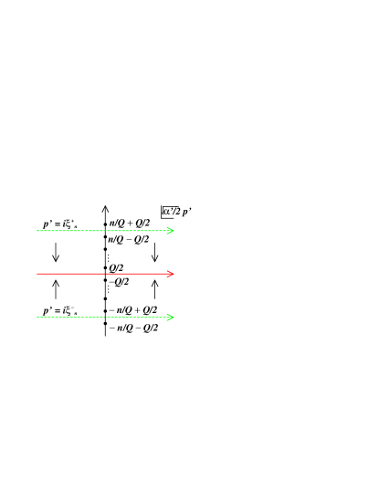
Figure 1: Deformation of the contour from the broken line to the solid line picks up pole contributions.

The relevant poles are located at

$$\sqrt{\frac{\alpha^{\prime}}{2}}p^{\prime}=i{\alpha_{m}}~{},~{}~{}~{}\alpha_{m}\equiv\frac{n}{Q}-Q\left(m+\frac{1}{2}\right)\quad\mbox{where}\quad m=0,1,\ldots,\left[\frac{n}{Q^{2}}-\frac{1}{2}\right]~{},\qquad\quad$$ (3.16)

where $[~{}~{}]$ denotes the Gauss symbol, and their residues are evaluated as $(-1)^{n+1}\frac{i}{\pi}e^{\pi t_{o}\alpha_{m}^{2}}$. We thus obtain

$$\int_{\mathbb{R}-i0}\sqrt{\frac{\alpha^{\prime}}{2}}{\rm d}p\,a^{+}_{n}(p)e^{-2\pi t_{c}\frac{\alpha^{\prime}}{4}p^{2}} = (-1)^{n+1}\frac{i\sqrt{t_{o}}}{Q}\int_{-\infty}^{\infty}\sqrt{\frac{\alpha^{\prime}}{2}}{\rm d}p^{\prime}\,\frac{e^{\pi\left(\sqrt{\frac{\alpha^{\prime}}{2}}\frac{p^{\prime}}{Q}-i\frac{n}{Q^{2}}\right)-2\pi t_{o}\frac{\alpha^{\prime}}{4}p^{{}^{\prime}2}}}{\cosh\pi\left(\sqrt{\frac{\alpha^{\prime}}{2}}\frac{p^{\prime}}{Q}-i\frac{n}{Q^{2}}\right)}$$ (3.17)

$$+ 2(-1)^{n+1}\sqrt{t_{o}}\sum_{m=0}^{\left[\frac{n}{Q^{2}}-\frac{1}{2}\right]}\,e^{\pi t_{o}\left[\frac{n}{Q}-Q\left(m+\frac{1}{2}\right)\right]^{2}}~{}.$$

The integral of $a^{-}_{n}(p)$ is calculated in a similar way. This time, we should start with the contour $\mathbb{R}+i\xi^{-}_{n}$ with $(-\frac{n}{Q}-\frac{Q}{2})<\sqrt{\frac{\alpha^{\prime}}{2}}\xi^{-}_{n}<(-\frac{n}{Q}+\frac{Q}{2})$ and, after performing the $p$-integral first, again shift it back to $\mathbb{R}+i\xi^{-}_{n}\,\rightarrow\,\mathbb{R}$. The relevant pole contributions come from $\sqrt{\frac{\alpha^{\prime}}{2}}p^{\prime}=-i\alpha_{m}$ ($m=0,1,\ldots,\left[\frac{n}{Q^{2}}-\frac{1}{2}\right]$), and we obtain

$$\int_{\mathbb{R}-i0}\sqrt{\frac{\alpha^{\prime}}{2}}{\rm d}p\,a^{-}_{n}(p)\,e^{-\pi t_{c}\alpha^{\prime}p^{2}} = (-1)^{n+1}\frac{i\sqrt{t_{o}}}{Q}\int_{-\infty}^{\infty}\sqrt{\frac{\alpha^{\prime}}{2}}{\rm d}p^{\prime}\,\frac{e^{\pi\left(\sqrt{\frac{\alpha^{\prime}}{2}}\frac{p^{\prime}}{Q}+i\frac{n}{Q^{2}}\right)-2\pi t_{o}\frac{\alpha^{\prime}}{4}p^{{}^{\prime}2}}}{\cosh\pi\left(\sqrt{\frac{\alpha^{\prime}}{2}}\frac{p^{\prime}}{Q}+i\frac{n}{Q^{2}}\right)}$$ (3.18)

$$- 2(-1)^{n+1}\sqrt{t_{o}}\sum_{m=0}^{\left[\frac{n}{Q^{2}}-\frac{1}{2}\right]}\,e^{\pi t_{o}\left[\frac{n}{Q}-Q\left(m+\frac{1}{2}\right)\right]^{2}}~{}.$$

Notice that the relative sign change in the pole term compared to $a^{+}_{n}(p)$ integral originates from the orientation of integration contour surrounding each pole. Therefore, we find

$$\int_{0}^{\infty}\sqrt{\frac{\alpha^{\prime}}{2}}{\rm d}p\,a_{n}(p)e^{-2\pi t_{c}\frac{\alpha^{\prime}}{4}p^{2}} = \frac{1}{2}\int_{-\infty}^{\infty}\sqrt{\frac{\alpha^{\prime}}{2}}{\rm d}p\,\left(a_{n}^{+}(p)-a_{n}^{-}(p)\right)e^{-2\pi\alpha^{\prime}\frac{t_{c}}{4}p^{2}}$$ (3.19)

$$= (-1)^{n+1}\frac{\sqrt{t_{o}}}{Q}\int_{-\infty}^{\infty}\sqrt{\frac{\alpha^{\prime}}{2}}{\rm d}p^{\prime}\,\frac{\sin\left(\frac{2\pi n}{Q^{2}}\right)e^{-2\pi t_{o}\frac{\alpha^{\prime}}{4}p^{{}^{\prime}2}}}{\cosh\left(\frac{2\pi}{Q}\sqrt{\frac{\alpha^{\prime}}{2}}p^{\prime}\right)+\cos\left(\frac{2\pi n}{Q^{2}}\right)}$$

$$+ 2(-1)^{n+1}\sqrt{t_{o}}\sum_{m=0}^{\left[\frac{n}{Q^{2}}-\frac{1}{2}\right]}\,e^{\pi t_{o}\left(\frac{n}{Q}-Q\left(m+\frac{1}{2}\right)\right)^{2}}~{}.$$

In this way, we derive the desired open string channel expression of the total radiation rate;

$$\overline{{\cal N}} = N^{2}_{\rm NS}\int_{0}^{\infty}\frac{{\rm d}t_{o}}{t_{o}}\,\Big{(}F_{\rm naive}(t_{o})+F_{\rm pole}(t_{o})\Big{)}~{},$$

$$F_{\rm naive}(t_{o}) = \frac{1}{Q}\int_{-\infty}^{\infty}\sqrt{\frac{\alpha^{\prime}}{2}}{\rm d}p^{\prime}\sum_{n=1}^{\infty}\,(-1)^{n+1}\frac{\sin\left(\frac{2\pi n}{Q^{2}}\right)e^{-\pi t_{o}\left(\frac{\alpha^{\prime}}{2}p^{{}^{\prime}2}+\frac{n^{2}}{Q^{2}}\right)}}{\cosh\left(\frac{2\pi}{Q}\sqrt{\frac{\alpha^{\prime}}{2}}p^{\prime}\right)+\cos\left(\frac{2\pi n}{Q^{2}}\right)}\,Z_{{\cal M}}^{(o)}(t_{o})$$

$$F_{\rm pole}(t_{o}) = 2\sum_{n=1}^{\infty}(-1)^{n+1}\sum_{m=0}^{\left[\frac{n}{Q^{2}}-\frac{1}{2}\right]}\,e^{\pi t_{o}\left[Q^{2}\left(m+\frac{1}{2}\right)^{2}-2n\left(m+\frac{1}{2}\right)\right]}\,Z_{{\cal M}}^{(o)}(t_{o})~{}.$$ (3.20)

The first term in (3.20) coincides with the total radiation claimed by [17] modulo inessential numerical factor . It remains finite as $t_{o}\,\rightarrow\,+\infty$. The second term, which the analysis of [17] missed altogether, is of crucial importance. It is evident that the $m=0$ term is the leading contribution for each $n$. Recalling $Z^{(o)}_{{\cal M}}(t_{o})\,\sim\,e^{\pi t_{o}\left(1-\frac{Q^{2}}{4}\right)}$ asymptotically (up to pre-exponential power corrections), each $m=0$ term behaves as

$$\sim e^{\pi t_{o}\left(\frac{Q^{2}}{4}-n\right)+\pi t_{o}\left(1-\frac{Q^{2}}{4}\right)}=e^{\pi t_{o}(1-n)}\qquad\mbox{as}\qquad t_{o}\,\rightarrow\,+\infty~{}.$$ (3.21)

Therefore, we get the leading contribution from the $n=1$ term, which shows a massless behavior. Hence, we have reproduced the Hagedorn-growth behavior expected in [12, 15, 13, 14]. Notice that all the $n>1$ contributions are massive, and thus are not relevant in the ultraviolet regime of closed string radiations.

3.3 Lorentzian cylinder amplitude

In the previous section, we recasted the total emission number $\overline{{\cal N}}$ of the rolling D0-brane, defined as the sum over the on-shell states of emitted closed string (3.5), in the open string channel. Now, by the optical theorem and the channel duality, we ought to be able to obtain $\overline{{\cal N}}$ equally well from the cylinder amplitude evaluated in the open channel. In this section, we shall compute explicitly the cylinder amplitude in the open string channel and show that its imaginary part reproduces precisely the result (3.20). This would serve as a non-trivial check-point of our previous analysis for the consistency with unitarity and the open-closed channel duality. Notice in particular that the channel duality is far from being obvious in the worldsheet in Lorentzian signature. For definiteness, we continue to focus on the NS sector.

We start with the cylinder amplitude with Lorentzian worldsheet  $Z_{\rm cylinder}$:

$$Z_{\rm cylinder}$$ (3.22)

$$= i\frac{\alpha^{\prime}}{2}\int_{s_{c}^{\rm UV}}^{s_{c}^{\rm IR}}{\rm d}s_{c}\int_{0}^{\infty}{\rm d}p\int_{-\infty}^{\infty}{\rm d}\omega_{L}\,\frac{\sinh\left(\frac{2\pi}{Q}\sqrt{\frac{\alpha^{\prime}}{2}}p\right)}{\left[\cosh\left(\frac{2\pi}{Q}\sqrt{\frac{\alpha^{\prime}}{2}}\omega_{L}\right)+\cosh\left(\frac{2\pi}{Q}\sqrt{\frac{\alpha^{\prime}}{2}}p\right)\right]\sinh(\pi Q\sqrt{\frac{\alpha^{\prime}}{2}}p)}$$

$$\hskip 85.35826pt\times\frac{q_{c}^{\frac{1}{4}\alpha^{\prime}(p^{2}-(1-i\hat{\epsilon})^{2}\omega_{L}^{2})}}{\eta(q_{c})^{2}}\frac{{\theta}_{3}(q_{c})}{\eta(q_{c})}\cdot Z_{{\cal M}}^{(c)}(q_{c})\cdot\eta(q_{c})^{2}\frac{\eta(q_{c})}{{\theta}_{3}(q_{c})}~{}.$$

Here, we again adopt the $i\epsilon$-prescription for the Lorentzian worldsheet, while the $-i\hat{\epsilon}$-prescription for the Lorentzian spacetime. The integration is well-defined so long as $2\hat{\epsilon}s_{c}^{\rm UV}>\epsilon>0$ is retained.

The second line in (3.22) combines contributions of the SL(2)_k/U(1), ${\cal M}$, and the worldsheet ghosts. The ghost contribution $\eta(q_{c})^{2}\frac{\eta(q_{c})}{{\theta}_{3}(q_{c})}$ is seen to cancel out the contribution of longitudinal oscillators. Thus, the amplitude simplifies to

$$\hskip 14.22636ptZ_{\rm cylinder}$$

$$= i\frac{\alpha^{\prime}}{2}\int_{s_{c}^{\rm UV}}^{s_{c}^{\rm IR}}{\rm d}s_{c}\int_{0}^{\infty}{\rm d}p\int_{-\infty}^{\infty}{\rm d}\omega_{L}\,\frac{\sinh\left(\frac{2\pi}{Q}\sqrt{\frac{\alpha^{\prime}}{2}}p\right)q_{c}^{\frac{1}{4}\alpha^{\prime}(p^{2}-(1-i\hat{\epsilon})^{2}\omega_{L}^{2})}\cdot Z_{{\cal M}}^{(c)}(q_{c})}{\left[\cosh\left(\frac{2\pi}{Q}\sqrt{\frac{\alpha^{\prime}}{2}}\omega_{L}\right)+\cosh\left(\frac{2\pi}{Q}\sqrt{\frac{\alpha^{\prime}}{2}}p\right)\right]\sinh(\pi Q\sqrt{\frac{\alpha^{\prime}}{2}}p)}~{}.$$

We now modular transform (LABEL:L_cylinder_closed) to the open string channel. Define again the open string modulus as $q_{o}=e^{-2\pi i\tau_{o}}$, where $\tau_{o}=s_{o}-i\epsilon$ and $s_{o}=1/s_{c}$. Using the Fourier transform identity:

$$\int_{-\infty}^{\infty}{\rm d}x\,\frac{\sin(\pi ax)}{\sinh(\pi x)}e^{-2\pi ikx}=\frac{\sinh(\pi a)}{\cosh(2\pi k)+\cosh(\pi a)}~{},\qquad(\left|\mbox{Im}\,a\right|<1)$$ (3.24)

we then obtain

$$\hskip 14.22636ptZ_{\rm cylinder}=$$

$$\hskip-22.76228pt\frac{i\alpha^{\prime}}{4}\int_{s_{o}^{\rm UV}}^{s_{o}^{\rm IR}}\frac{{\rm d}s_{o}}{s_{o}}\int_{-\infty}^{\infty}{\rm d}p^{\prime}\int_{-\infty}^{\infty}{\rm d}\omega_{L}^{\prime}\,\frac{\sinh\left(\frac{2\pi}{Q}\sqrt{\frac{\alpha^{\prime}}{2}}\omega^{\prime}_{L}\right)q_{o}^{\frac{1}{4}\alpha^{\prime}(p^{{}^{\prime}2}-(1+i\hat{\epsilon}^{\prime})^{2}\omega_{L}^{{}^{\prime}2})}\cdot Z_{{\cal M}}^{(o)}(q_{o})}{\left[\cosh\left(\frac{2\pi}{Q}\sqrt{\frac{\alpha^{\prime}}{2}}\omega^{\prime}_{L}\right)+\cosh\left(\frac{2\pi}{Q}\sqrt{\frac{\alpha^{\prime}}{2}}p^{\prime}\right)\right]\sinh(\pi Q\sqrt{\frac{\alpha^{\prime}}{2}}\omega_{L}^{\prime})}.\,\,\,\,\,\,$$

(3.25)

Again $s_{o}^{\rm UV}\equiv 1/s_{c}^{\rm IR}$, $s_{o}^{\rm IR}\equiv 1/s_{c}^{\rm UV}$ are the cut-off’s and the expression (3.25) is well-defined so long as $2\hat{\epsilon}^{\prime}s_{o}^{\rm UV}>\epsilon$.

3.4 analytic continuation

We shall now analytically continue both the spacetime and the worldsheet to the Euclidean signature. We have to carefully make the continuation so that keeping the original amplitude (3.25) unchanged (up to cut-off’s). As in the previous section, we should first Wick rotate in spacetime $\omega^{\prime}_{L}\,\rightarrow\,e^{i(\frac{\pi}{2}-0)}\omega^{\prime}_{L}$ with $\omega^{\prime}_{L}=i\omega^{\prime}$ $(\omega^{\prime}\in\mathbb{R})$, and then rotate the worldsheet $s_{o}\,\rightarrow\,-it_{o}$ ($t>0$). We shall omit the cutoff’s from now on. We reach the expression

$$Z_{\rm cylinder}=Z_{\rm naive}+Z_{\rm pole}~{},$$ (3.26)

where the first part is the contribution from naive continuation, while the second parts originates from the poles passed over by the rotated contour: $\omega^{\prime}_{L}\,\rightarrow\,e^{i(\frac{\pi}{2}-0)}\omega^{\prime}_{L}$. See Figure 2.

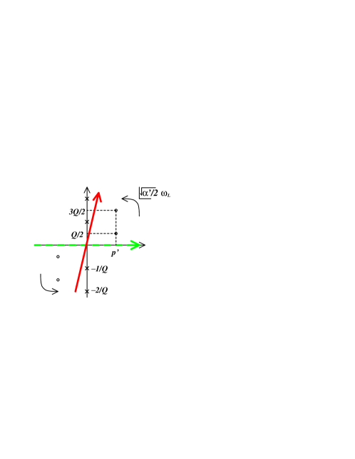
Figure 2: The $\omega_{L}$-integral with Lorentzian contour (broken line) and the Euclidean contour (solid line).

The first part $Z_{\rm naive}$ is given by

$$\hskip 5.69046ptZ_{\rm naive}=$$

$$\hskip-28.45274pt\int_{0}^{\infty}\frac{{\rm d}t_{o}}{t_{o}}\int_{-\infty}^{\infty}\!\!{\rm d}p^{\prime}\int_{(1-i0)\mathbb{R}}\!\!\!\!\!{\rm d}\omega^{\prime}\,\frac{-\frac{1}{4}\alpha^{\prime}\sin\left(\frac{2\pi}{Q}\sqrt{\frac{\alpha^{\prime}}{2}}\omega^{\prime}\right)q_{o}^{\frac{1}{4}\alpha^{\prime}(p^{{}^{\prime}2}+\omega^{{}^{\prime}2})}\cdot Z_{{\cal M}}^{(o)}(q_{o})}{\left[\cos\left(\frac{2\pi}{Q}\sqrt{\frac{\alpha^{\prime}}{2}}\omega^{\prime}\right)+\cosh\left(\frac{2\pi}{Q}\sqrt{\frac{\alpha^{\prime}}{2}}p^{\prime}\right)\right]\sin(\pi Q\sqrt{\frac{\alpha^{\prime}}{2}}\omega^{\prime})}~{}.\quad$$ (3.27)

The second part $Z_{\rm pole}$ arises from the poles located at

$$\sqrt{\frac{\alpha^{\prime}}{2}}\omega^{\prime}_{L}=\left\{\begin{array}[]{ll}\sqrt{\frac{\alpha^{\prime}}{2}}|p^{\prime}|+{iQ}\left(m+\frac{1}{2}\right)&~{}~{}m\in\mathbb{Z}_{\geq 0}\\ -\sqrt{\frac{\alpha^{\prime}}{2}}|p^{\prime}|+{iQ}\left(m+\frac{1}{2}\right)&~{}~{}m\in\mathbb{Z}_{<0}\end{array}\right.$$ (3.30)

whose residues are (after taking the open string channel modulus Euclidean, $q_{o}=e^{-2\pi t}$)

$$\frac{i}{2}\sqrt{\frac{2}{\alpha^{\prime}}}\cdot\frac{Q}{2\pi}\frac{e^{\pm i\pi tQ(2m+1)\sqrt{\frac{\alpha^{\prime}}{2}}|p^{\prime}|-\pi tQ^{2}\left(m+\frac{1}{2}\right)^{2}}}{\sinh\pi Q\left(\pm\sqrt{\frac{\alpha^{\prime}}{2}}|p^{\prime}|+iQ\left(m+\frac{1}{2}\right)\right)}~{}.$$ (3.31)

We thus obtain

$$Z_{\mbox{\scriptsize pole}}=\int_{0}^{\infty}\frac{{\rm d}t_{o}}{t_{o}}\,\left[\sum_{m\geq 0}\int_{0}^{\infty}\sqrt{\frac{\alpha^{\prime}}{2}}{\rm d}p^{\prime}-\sum_{m<0}\int_{-\infty}^{0}\sqrt{\frac{\alpha^{\prime}}{2}}{\rm d}p^{\prime}\right]\,{e^{i\pi tQ(2m+1)\sqrt{\frac{\alpha^{\prime}}{2}}p^{\prime}-\pi tQ^{2}\left(m+\frac{1}{2}\right)^{2}}}$$

$$\hskip 85.35826pt\times 2\pi i\cdot\frac{iQ}{4\pi}\left[\frac{1}{\sinh\pi Q\left(\sqrt{\frac{\alpha^{\prime}}{2}}p^{\prime}+iQ\left(m+\frac{1}{2}\right)\right)}+(p^{\prime}\leftrightarrow-p^{\prime})\right]Z_{{\cal M}}^{(o)}(q_{o})$$

$$\hskip 28.45274pt=-2Q\int_{0}^{\infty}\frac{{\rm d}t_{o}}{t_{o}}\,\sum_{m=0}^{\infty}\int_{0}^{\infty}\sqrt{\frac{\alpha^{\prime}}{2}}{\rm d}p^{\prime}\,\frac{e^{i\pi tQ(2m+1)\sqrt{\frac{\alpha^{\prime}}{2}}p^{\prime}-\pi tQ^{2}\left(m+\frac{1}{2}\right)^{2}}}{\sinh\pi Q\left(\sqrt{\frac{\alpha^{\prime}}{2}}p^{\prime}+iQ\left(m+\frac{1}{2}\right)\right)}\cdot Z_{{\cal M}}^{(o)}(q_{o})~{}.$$

(3.32)

We thus obtained manifestly convergent open string channel expressions (3.27), (3.32) for the cylinder amplitude in Lorentzian signature of the spacetime.

3.5 optical theorem at work

With the Lorentzian (in spacetime) cylinder amplitude (3.27), (3.32) available, we now apply the unitarity and obtain total emission number $\overline{\cal N}$ via imaginary part of $Z_{\rm cylinder}$. In the analysis of [17] only the naive contribution $Z_{\mbox{\scriptsize naive}}$ was considered. Taking the imaginary part picks up infinite poles located at the real $\omega^{\prime}$-axis (the imaginary $\omega^{\prime}_{L}$-axis), depicted in Figure 2. Their contributions yield

$$\mbox{Im}\,Z_{\mbox{\scriptsize naive}}$$ (3.33)

$$= -\frac{1}{2}\int_{0}^{\infty}\frac{{\rm d}t_{o}}{t_{o}}\int_{-\infty}^{\infty}\sqrt{\frac{\alpha^{\prime}}{2}}{\rm d}p^{\prime}\sum_{\stackrel{{\scriptstyle n\neq 0}}{{n\in\mbox{\scriptsize{\bf Z}}}}}\,\pi\mbox{sgn}\,(n)\,\frac{(-1)^{n}}{\pi Q}\frac{\sin\left(\frac{2\pi n}{Q^{2}}\right)e^{-\pi t\left(\frac{\alpha^{\prime}}{2}p^{{}^{\prime}2}+\frac{n^{2}}{Q^{2}}\right)}}{\cos\left(\frac{2\pi n}{Q^{2}}\right)+\cosh\left(\frac{2\pi}{Q}\sqrt{\frac{\alpha^{\prime}}{2}}p^{\prime}\right)}\cdot Z_{{\cal M}}^{(o)}(q_{o})$$

$$= -\sum_{n=1}^{\infty}\int_{0}^{\infty}\frac{{\rm d}t_{o}}{t_{o}}\int_{-\infty}^{\infty}\sqrt{\frac{\alpha^{\prime}}{2}}{\rm d}p^{\prime}\,\frac{(-1)^{n}}{Q}\frac{\sin\left(\frac{2\pi n}{Q^{2}}\right)e^{-\pi t\left(\frac{\alpha^{\prime}}{2}p^{{}^{\prime}2}+\frac{n^{2}}{Q^{2}}\right)}}{\cos\left(\frac{2\pi n}{Q^{2}}\right)+\cosh\left(\frac{2\pi}{Q}\sqrt{\frac{\alpha^{\prime}}{2}}p^{\prime}\right)}\cdot Z_{{\cal M}}^{(o)}(q_{o})~{},$$

reproducing the first term in (3.20).

We next evaluate the contribution from the pole contribution $Z_{\mbox{\scriptsize pole}}$ (3.32). As is easily seen, taking the imaginary part just amounts to extending the integration region of $p^{\prime}$ in (3.32) to the whole real axis $(-\infty,\infty)$. By closing the $p^{\prime}$-contour in the upper half plane, we thus obtain

$$\mbox{Im}\,Z_{\mbox{\scriptsize pole}}$$ (3.34)

$$= iQ\int_{0}^{\infty}\frac{{\rm d}t_{o}}{t_{o}}\,\sum_{m=0}^{\infty}\int_{-\infty}^{\infty}\sqrt{\frac{\alpha^{\prime}}{2}}{\rm d}p^{\prime}\,\frac{e^{i\pi tQ(2m+1)\sqrt{\frac{\alpha^{\prime}}{2}}p^{\prime}-\pi tQ^{2}\left(m+\frac{1}{2}\right)^{2}}}{\sinh\pi Q\left(\sqrt{\frac{\alpha^{\prime}}{2}}p^{\prime}+iQ\left(m+\frac{1}{2}\right)\right)}\cdot Z_{{\cal M}}^{(o)}(q_{o})$$

$$= 2\pi i\cdot iQ\int_{0}^{\infty}\frac{{\rm d}t_{o}}{t_{o}}\,\sum_{m=0}^{\infty}\sum_{\stackrel{{\scriptstyle n>Q^{2}\left(m+\frac{1}{2}\right)}}{{n\in\mbox{\scriptsize{\bf Z}}_{>0}}}}\,\frac{(-1)^{n}}{\pi Q}e^{-\pi tn(2m+1)+\pi tQ^{2}\left(m+\frac{1}{2}\right)^{2}}\cdot Z_{{\cal M}}^{(o)}(q_{o})$$

$$= -2\int_{0}^{\infty}\frac{{\rm d}t_{o}}{t_{o}}\,\sum_{n=1}^{\infty}\sum_{m=0}^{\left[\frac{n}{Q^{2}}-\frac{1}{2}\right]}\,(-1)^{n}e^{-\pi tn(2m+1)+\pi tQ^{2}\left(m+\frac{1}{2}\right)^{2}}\cdot Z_{{\cal M}}^{(o)}(q_{o})~{}.$$

In the last line, we exchanged order of the double summations. The final result agrees perfectly with the total emission number $\overline{\cal N}$ in (3.20) evaluated via direct computation of the transition amplitudes in Euclidean worldsheet.

4 Interpretations and Discussions

In the previous sections, we studied spectral observables in causal processes involving decay of unstable D-brane and rolling of accelerated D-brane. The main result of this work is that transformation of the total emission number $\overline{\cal N}$ and the cylinder amplitude $Z_{\rm cylinder}$ from the closed string channel to the open string channel require careful analytic continuation on the worldsheet and that, unlike other results claimed in the literatures, the analytic continuation we adopt gives results consistent with the unitarity via the optical theorem $\overline{\cal N}=\mbox{Im}\,Z_{\rm cylinder}$. In particular, we found that the cylinder amplitude consists in general of two parts $Z_{\rm cylinder}=Z_{\rm naive}+Z_{\rm pole}$, and the second part is crucial for ensuring the unitarity through its imaginary part. While we dealt with decaying or rolling process of the D-brane, the rules we developed ought to extend to other real-time processes such as open string and D-brane dynamics in electric field or plane-wave field background.

In this section, we highlights several impotant steps we noted in establishing consistency between the channel duality and the unitarity.

4.1 imaginary D-instantons: decaying versus rolling

Throughout this work, the strategy for recasting the closed string emission spectra in open string channel was to expand the transition probability ${\cal P}(\omega,{\bf p})$ in power series of ‘imaginary D-instantons’ [31, 18, 32], viz. contributions of localized states at time $2\pi i\alpha^{\prime}W(m,n)$ for decaying D-branes and at time $(2\pi i/Q)n\sqrt{\frac{\alpha^{\prime}}{2}}$ for rolling D-branes, respectively.

A crucial difference we noted for the rolling D-brane in NS5-brane background, $Q<\sqrt{2}$, that weight of the $n$-th imaginary D-instanton, $a_{n}(p)$, is a non-trivial function of $p$. We emphasized above that the momentum dependence came about because accelerated D-brane rolls in the two-dimensional subspace $\mathbb{R}_{t}\times\mathbb{R}_{\phi}$. Being process dependent, it could be that, in general, the weights are exponentially growing functions of momentum, and their Fourier transformations are not necessarily well-defined. This was indeed the case for the rolling D-brane case. We thus prescribed the Fourier transform of the D-instanton weight by analytic continuation via a deformed integration contour. The prescription then yielded in the open string channel the contribution $Z_{\rm pole}$ beyond the naive one $Z_{\rm naive}$. Moreover, whereas the naive contribution is always ultraviolet finite, the pole contribution exhibited ultraviolet divergence. Since $\overline{\cal N}$ (or higher spectral moment) is ultraviolet divergent, we concluded that the presence of ultraviolet divergent $Z_{\rm pole}$ is crucial for consistency with the unitarity and the channel duality.

From mathematical viewpoint, we found that the pole contribution $Z_{\rm pole}$ in (3.20) is present in so far as we adopt mathematically well-posed prescription of the Fourier transform. ¿From physics viewpoint, we can also argue that the first term $Z_{\rm naive}$ by itself cannot be the correct answer and the second term $Z_{\rm pole}$ ought to dominate over the first one.

In the range $Q<\sqrt{2}$, it is easy to see that $\mbox{Im}\,Z_{\rm naive}$ can take a negative value if we tune the value $Q$ suitably within this range. If $Z_{\rm naive}$ is all there is for the cylinder amplitude, the negative value of its imaginary part contradicts with the fact that the total emission number $\overline{\cal N}$ is positive by definition. Moreover, for $Q=\sqrt{2/k}$ $k\in\mathbb{Z}_{>1}$, which corresponds to rolling D-branes in $k$ coincident NS5 backgrounds, we observe that the first term $Z_{\rm naive}$ vanishes identically since the integrand vanishes. The above observations indicate that extra contribution ought to be present to the cylinder amplitude beyond the naive contribution, $Z_{\rm naive}$.

On other other hand, we do not have any contradiction of the cylinder amplitude with the unitarity once the contribution $Z_{\rm pole}$ is taken into account. This is because $Z_{\rm pole}$ is dominant (generically divergent) over $Z_{\rm naive}$ and always positive. We conclude that our prescription for the cylinder amplitude renders the total emission number, as extracted from the optical theorem as $\overline{\cal N}=\mbox{Im}\,Z$ always positive and well-defined.

The situation is in sharp contrast to that for decaying D-brane case. There, as recapitulated in section 2, the D-instanton weights were constant ($a_{n,m}=1$), so the issue of Fourier transform was void from the outset. Again, as explained in section 2, the momentum independence came about because unstable D-brane decays at rest (or trivially Lorentz boosted). The situation in NS5-brane phase $Q<\sqrt{2}$ is also in contrast to that in the ’fundamental string phase’ [25], $\sqrt{2}<Q\leq 2$, or in ‘out-going’ radiation in nonextremal NS5-brane background (which involves two-dimensional black hole geometry) [14]. For these, the leading weight $a_{1}(p)$ is a bounded function and have well-defined Fourier transformation. So, there does not arise any extra contribution beyond $Z_{\rm naive}$. We thus obtain via optical theorem an ultraviolet finite total emission number .

In the previous work [14], we also noted that the first D-instanton weight $a_{1}(p)$ is identifiable with the ‘grey body factor’ $\sigma(p)$ in the total emission number $\overline{\cal N}$. There, the identification was based on saddle-point analysis valid at large mass $M\rightarrow\infty$ in the closed string channel. The present result in the open string channel, where the leading ultraviolet divergence arises from the weight $a_{1}(p)$, then supports the identification .

4.2 comparisons

From our analysis, it became clear the reason why [19] obtained the correct result for the decay of unstable D-brane is because the contour rotation in Fourier transform did not encounter any pole (since the D-instanton weights $a_{n}(p)$ were $p$-independent constants), and the naive manipulation yielded the correct result. In [17], the prescription of [19] was taken literally also for the rolling of accelerated D-brane. It was then concluded that $Z_{\rm naive}$ refers to the total cylinder amplitude. We showed throughout this work that this is incorrect since it overlooked the pole contribution $Z_{\rm pole}$. After all, only after taking this extra contribution into account, we showed that the cylinder amplitude is consistent with the channel duality and the unitarity.

Finally, we find it illuminating to understand why $\overline{\cal N}$ exhibited Hagedorn divergence in the two-dimensional string theory studied in [20], whereas it is ultraviolet finite in the linear dilaton background studied in [19] in two-dimensional spacetime (that is, $c_{\mbox{\scriptsize eff}}=0$). The reason is because the boundary wave function (D-brane transition amplitude) of the former has non-trivial $p$-dependence that exponentially diverges, whereas the latter does not.

Acknowledgement

We thank David J. Gross and Jung-Tay Yee for useful discussions, and acknowledge Kazumi Okuyama and Moshe Rozali for correspondences. YN’s work was supported in part by JSPS Research Fellowship for Young Scientists. SJR’s work was supported in part by the KOSEF SRC Program ”Center for Quantum Spacetime” (R11-2005-021). YS’s work was supported in part by the Ministry of Education, Culture, Sports, Science and Technology of Japan.

References

• [1] See, for example, chapter 6 of C. Itzykson and B. Zuber, ”Quantum Field Theory” (McGraw-Hill Pub. Co, 1980, New York).
• [2] T. G. Erler and D. J. Gross, arXiv:hep-th/0406199.
• [3] M. Gutperle and A. Strominger, Phys. Rev. D 67, 126002 (2003) [arXiv:hep-th/0301038]; A. Strominger and T. Takayanagi, Adv. Theor. Math. Phys.  7, 369 (2003) [arXiv:hep-th/0303221]; V. Schomerus, JHEP 0311, 043 (2003) [arXiv:hep-th/0306026].
• [4] V. Balasubramanian, S. F. Hassan, E. Keski-Vakkuri and A. Naqvi, Phys. Rev. D 67, 026003 (2003) [arXiv:hep-th/0202187]; L. Cornalba and M. S. Costa, Phys. Rev. D 66, 066001 (2002) [arXiv:hep-th/0203031]; J. Simon, JHEP 0206, 001 (2002) [arXiv:hep-th/0203201]; N. A. Nekrasov, Surveys High Energ. Phys.  17, 115 (2002) [arXiv:hep-th/0203112], H. Liu, G. W. Moore and N. Seiberg, JHEP 0206, 045 (2002) [arXiv:hep-th/0204168]; ibid. JHEP 0210, 031 (2002) [arXiv:hep-th/0206182].
• [5] S. Elitzur, A. Giveon, D. Kutasov and E. Rabinovici, JHEP 0206, 017 (2002) [arXiv:hep-th/0204189]; B. Craps, D. Kutasov and G. Rajesh, JHEP 0206, 053 (2002) [arXiv:hep-th/0205101]; M. Berkooz, B. Craps, D. Kutasov and G. Rajesh, JHEP 0303, 031 (2003) [arXiv:hep-th/0212215].
• [6] C. Bachas and M. Porrati, Phys. Lett. B 296, 77 (1992) [arXiv:hep-th/9209032]; B. Pioline and M. Berkooz, JCAP 0311, 007 (2003) [arXiv:hep-th/0307280].
• [7] C. Bachas and C. Hull, JHEP 0212, 035 (2002) [arXiv:hep-th/0210269]; R. C. Myers and D. J. Winters, JHEP 0212, 061 (2002) [arXiv:hep-th/0211042]; K. Okuyama, JHEP 0302, 043 (2003) [arXiv:hep-th/0211218]; C. Bachas, Annals Phys.  305, 286 (2003) [arXiv:hep-th/0212217]; B. Durin and B. Pioline, JHEP 0305, 035 (2003) [arXiv:hep-th/0302159]; Y. Hikida, H. Takayanagi and T. Takayanagi, JHEP 0304, 032 (2003) [arXiv:hep-th/0303214].
• [8] A. Sen, JHEP 0204, 048 (2002) [arXiv:hep-th/0203211], JHEP 0207, 065 (2002) [arXiv:hep-th/0203265]; M. Gutperle and A. Strominger, JHEP 0204, 018 (2002) [arXiv:hep-th/0202210]; A. Strominger, arXiv:hep-th/0209090.
• [9] D. Kutasov, arXiv:hep-th/0405058.
• [10] S. M. Lee and S. J. Rey, Nucl. Phys. B 508, 107 (1997) [arXiv:hep-th/9706115].
• [11] D. Bak, S. J. Rey and H. U. Yee, JHEP 0412, 008 (2004) [arXiv:hep-th/0411099].
• [12] Y. Nakayama, Y. Sugawara and H. Takayanagi, JHEP 0407, 020 (2004) [arXiv:hep-th/0406173].
• [13] Y. Nakayama, K. L. Panigrahi, S. J. Rey and H. Takayanagi, JHEP 0501, 052 (2005) [arXiv:hep-th/0412038].
• [14] Y. Nakayama, S. J. Rey and Y. Sugawara, JHEP 0509, 020 (2005) [arXiv:hep-th/0507040].
• [15] D. A. Sahakyan, JHEP 0410, 008 (2004) [arXiv:hep-th/0408070].
• [16] B. Chen, M. Li and B. Sun, JHEP 0412, 057 (2004) [arXiv:hep-th/0412022];
• [17] K. Okuyama and M. Rozali, arXiv:hep-th/0602060. JHEP 0603, 071 (2006) [arXiv:hep-th/0602060].
• [18] N. Lambert, H. Liu and J. Maldacena, arXiv:hep-th/0303139.
• [19] J. L. Karczmarek, H. Liu, J. Maldacena and A. Strominger, JHEP 0311, 042 (2003) [arXiv:hep-th/0306132].
• [20] I. R. Klebanov, J. Maldacena and N. Seiberg, JHEP 0307, 045 (2003) [arXiv:hep-th/0305159].
• [21] D. Kutasov and N. Seiberg, Nucl. Phys. B 358, 600 (1991).
• [22] V. Fateev, A. B. Zamolodchikov and A. B. Zamolodchikov, arXiv:hep-th/0001012.
• [23] Y. Nakayama, Int. J. Mod. Phys. A 19, 2771 (2004) [arXiv:hep-th/0402009].
• [24] A. B. Zamolodchikov and A. B. Zamolodchikov, arXiv:hep-th/0101152.
• [25] A. Giveon, D. Kutasov, E. Rabinovici and A. Sever, arXiv:hep-th/0503121.
• [26] S. J. Rey, Phys. Rev. D 43, 526 (1991); ibid. ”Axionic String Instantons and Their Low-Energy Implications”, UCSB-TH-89/49, in the proceedings of the ”Workshop on Superstrings and Particle Theory” pp. 291-300 (World Scientific Pub., 1989).
• [27] C. G. . Callan, J. A. Harvey and A. Strominger, Nucl. Phys. B 359, 611 (1991); S. J. Rey, ”On String Theory and Axionic Strings and Instantons”, SLAC-PUB-5659, in the proceedings of ”Particle and Fields ’91 Conference” pp. 876-881 (American Physical Society, 1991).
• [28] S. Ribault and V. Schomerus, JHEP 0402, 019 (2004) [arXiv:hep-th/0310024]; T. Eguchi and Y. Sugawara, JHEP 0401, 025 (2004) [arXiv:hep-th/0311141]; C. Ahn, M. Stanishkov and M. Yamamoto, Nucl. Phys. B 683, 177 (2004) [arXiv:hep-th/0311169]; S. L. Lukyanov, E. S. Vitchev and A. B. Zamolodchikov, Nucl. Phys. B 683, 423 (2004) [arXiv:hep-th/0312168].
• [29] D. Kutasov, arXiv:hep-th/0509170.
• [30] J. Polchinski, Commun. Math. Phys.  104, 37 (1986); B. Sathiapalan, Phys. Rev. D 35, 3277 (1987); Y. I. Kogan, JETP Lett.  45, 709 (1987) [Pisma Zh. Eksp. Teor. Fiz.  45, 556 (1987)]; K. H. O’Brien and C. I. Tan, Phys. Rev. D 36, 1184 (1987); J. J. Atick and E. Witten, Nucl. Phys. B 310, 291 (1988).
• [31] A. Maloney, A. Strominger and X. Yin, JHEP 0310, 048 (2003) [arXiv:hep-th/0302146].
• [32] D. Gaiotto, N. Itzhaki and L. Rastelli, Nucl. Phys. B 688, 70 (2004) [arXiv:hep-th/0304192].