YITP-06-17

hep-th/0604194

One-loop unitarity of scalar field theories on Poincaré invariant commutative nonassociative spacetimes

Yuya Sasai and  Naoki Sasakura

Yukawa Institute for Theoretical Physics, Kyoto University,
Kyoto 606-8502, Japan

We study scalar field theories on Poincaré invariant commutative nonassociative spacetimes. We compute the one-loop self-energy diagrams in the ordinary path integral quantization scheme with Feynman’s prescription, and find that the Cutkosky rule is satisfied. This property is in contrast with that of noncommutative field theory, since it is known that noncommutative field theory with space/time noncommutativity violates unitarity in the above standard scheme, and the quantization procedure will necessarily become complicated to obtain a sensible Poincaré invariant noncommutative field theory. We point out a peculiar feature of the non-locality in our nonassociative field theories, which may explain the property of the unitarity distinct from noncommutative field theories. Thus commutative nonassociative field theories seem to contain physically interesting field theories on deformed spacetimes.

1 Introduction

Noncommutative spacetime is spacetime with noncommutative spacetime coordinates [1]-[4]. Since there appears uncertainty in non-commuting directions, noncommutative spacetime can be considered as an interesting candidate for new notion of quantum spacetime. Field theories on noncommutative spacetime are obtained from replacing commutative $C^{\ast}$-algebras of functions with noncommutative algebras [5].

It is known that noncommutative field theories are related to string theory and quantum gravity. In string theory, for example, noncommutative field theory is an effective theory, which is obtained in the $\alpha^{\prime}\to 0$ limit of the open string theory with constant background $B_{\mu\nu}$ field [6]. In quantum gravity, for example, the effective dynamics of quantum particles coupled to three-dimensional quantum gravity can be expressed in terms of an effective noncommutative field theory which respects the principles of doubly special relativity [7].

But some noncommutative field theories do not respect the principles of special relativity or quantum mechanics. The simplest example is the spacetime with the noncommutativity $[x^{\mu},x^{\nu}]=i\theta^{\mu\nu}$, where $\theta^{\mu\nu}$ is a constant antisymmetric tensor. The field theory on the noncommutative spacetime does not have the ordinary Lorentz symmetry except in two-dimensions, since $\theta^{\mu\nu}$ is not Lorentz invariant, while recent developments show that noncommutative field theory has twisted Poincaré symmetry [8, 9]. It is not unitary in the standard path integral quantization procedure with Feynman’s prescription, when it has space/time noncommutativity [10]-[12]. In [10], this was shown by computing explicitly the one-loop amplitudes and showing the violation of the Cutkosky rule. Also it is known that acausal effects occur, when it has space/time noncommutativity [15]. Moreover, it has an unusual behavior, called UV-IR mixing, that the ultra-violet divergences appear in the limit of vanishing external momenta [16]-[18].

Is it possible to construct field theories on deformed spacetime which preserve both Lorentz symmetry and unitarity? Since Lorentz symmetry mixes space and time directions, the known facts in the preceding paragraph suggest that it becomes necessarily complicated for noncommutative spacetime. In this paper, we pursue the possibility of nonassociative spacetime. In fact, nonassociativity is known to appear in open string theory with non-constant background $B_{\mu\nu}$ field [19]. It was also argued that the algebra of closed string field theory should be commutative nonassociative [20]. There are also other discussions on nonassociative theory [21, 22]. Especially in [23], they discussed commutative nonassociative gauge theory with Lorentz symmetry.

This paper is organized as follows. In the following section we study scalar $\phi^{3}$ field theory obtained from the commutative nonassociative product,

$$\phi(x)\ast\phi(x)=e^{-\alpha(\partial_{a}+\partial_{b})^{2}}\phi(x+a)\phi(x+b)|_{a=b=0},$$

where $\alpha$ is a constant nonassociative deformation parameter. This product is obviously Poincaré invariant. Since this product contains an infinite number of space-time derivatives, unitarity seems to be a non-trivial issue. We find that this field theory satisfies the Cutkosky rule for the one-loop self-energy diagram.

In Section 3 we replace the above commutative nonassociative product to avoid a divergence in the amplitude. In fact the real part of the one-loop amplitude diverges exponentially in Minkowski spacetime, when we adopt the above product. This divergence is irrelevant to the discussions about the one-loop unitarity in Section 2, but may harm the significance of the field theory based on the above product. Thus we change the square of momenta on the exponential to the forth power, and study the field theory based on the new product. We check the one-loop Cutkosky rule to some orders of $\alpha$, and find the unitarity holds also in this case.

In Section 4 we discuss scalar field theories obtained from Poincaré invariant commutative associative algebras, and find that the couplings become constant in general. This shows that non-trivial behaviors of scalar field theories can appear only when commutativity or associativity of algebras is lost.

The final section is devoted to discussions and comments. We make an observation concerning the reason why our nonassociative field theories satisfy the unitarity relation from the viewpoint of a qualitative difference in non-locality between noncommutative field theories and our commutative nonassociative field theories.

2 Nonassociative $\phi^{3}$ theory: quadratic case

Noncommutative field theories can be constructed from replacing the usual multiplication of fields in the Lagrangian with Moyal product,

$$\phi(x)\ast\phi(x)=e^{\frac{i}{2}\theta^{\mu\nu}\frac{\partial}{\partial a^{\mu}}\frac{\partial}{\partial b^{\nu}}}\phi(x+a)\phi(x+b)|_{a=b=0}.$$ (1)

Then the spacetime noncommutativity is given by

$$[x^{\mu},x^{\nu}]=x^{\mu}\ast x^{\nu}-x^{\nu}\ast x^{\mu}=i\theta^{\mu\nu}.$$ (2)

This spacetime noncommutativity breaks Lorentz symmetry except in two dimensions. Moreover field theory with space/time noncommutativity ($\theta^{0i}\neq 0$) is not unitary in the standard path integral scheme [10]-[12].

The purpose of this paper is to pursue unitary field theories on deformed spacetimes with Lorentz symmetry. As candidates, we are going to construct scalar field theories on Poincaré invariant commutative nonassociative spacetimes and check the one-loop unitarity.

Let us first define the following commutative nonassociative star product,

$$\phi(x)\ast\phi(x)=e^{-\alpha(\partial_{a}+\partial_{b})^{2}}\phi(x+a)\phi(x+b)|_{a=b=0},$$ (3)

where $\alpha$ is a constant nonassociative deformation parameter. This parameter is taken to be real for the tree level unitarity to hold.

For the plane waves, the product (3) becomes

$$e^{ipx}\ast e^{iqx}=e^{\alpha(p+q)^{2}}e^{i(p+q)x}.$$ (4)

This is obviously Poincaré invariant, since it preserves the Lorentz symmetry and the momentum conservation. One can easily check that this product is commutative but nonassociative,

$$e^{ip_{1}x}\ast e^{ip_{2}x} =e^{ip_{2}x}\ast e^{ip_{1}x},$$

$$(e^{ip_{1}x}\ast e^{ip_{2}x})\ast e^{ip_{3}x} \neq e^{ip_{1}x}\ast(e^{ip_{2}x}\ast e^{ip_{3}x}).$$ (5)

Field theories based on the product will have features quite different from the noncommutative field theory based on the Moyal product.

Let us construct $\phi^{3}$ scalar field theory based on the above commutative nonassociative product. The action is defined by

$$S=\int d^{D}x\bigg{[}\frac{1}{2}\partial_{\mu}\phi(x)\ast\partial^{\mu}\phi(x)-\frac{1}{2}m^{2}\phi(x)\ast\phi(x)-\frac{g}{3!}\phi(x)\ast(\phi(x)\ast\phi(x))\bigg{]}.$$ (6)

The term $(\phi\ast\phi)\ast\phi$ is not necessary, because $(\phi\ast\phi)\ast\phi=\phi\ast(\phi\ast\phi)$ holds from the commutativity.

In this paper, we employ the standard path integral quantization procedure for the action (6). To find the Feynman rules, let us consider the Fourier transform of the field $\phi(x)$,

$$\phi(x)=\int_{p}\tilde{\phi}(p)\ e^{ipx},$$ (7)

where $\int_{p}=\int d^{D}p/(2\pi)^{D}$. The scalar field $\phi(x)$ is assumed to be real, and therefore $\tilde{\phi}(p)^{\ast}=\tilde{\phi}(-p)$. Substituting (7) into the action, we obtain

$$S =\int_{p}\frac{1}{2}(p^{2}-m^{2})\tilde{\phi}(p)\tilde{\phi}(-p)$$

$$\ \ \ \ -\frac{g}{3!}\int_{p}\int_{q}\int_{k}e^{\alpha(q+k)^{2}}e^{\alpha(p+(q+k))^{2}}\tilde{\phi}(p)\tilde{\phi}(q)\tilde{\phi}(k)(2\pi)^{D}\delta^{D}(p+q+k)$$

$$=\int_{p}\frac{1}{2}(p^{2}-m^{2})\tilde{\phi}(p)\tilde{\phi}(-p)-\frac{g}{3!}\int_{p}\int_{q}e^{\alpha p^{2}}\tilde{\phi}(p)\tilde{\phi}(q)\tilde{\phi}(-p-q).$$ (8)

One can read Feynman rules from (8). The Feynman rule for the propagator is given by the usual one as in Figure 1. Averaging over the orderings of the legs, the Feynman rule of the three-point vertex is given by Figure 2.

Figure 1: Propagator

Figure 2: Three-point vertex

Formal discussions on the quantization of the system respecting the structure of the star product will be given below.

Generating functional is defined by

$$W[J] =\int[d\phi]\exp{\bigg{\{}i\int d^{D}x\bigg{(}\frac{1}{2}\partial_{\mu}\phi\ast\partial^{\mu}\phi-\frac{1}{2}(m^{2}-i\epsilon)\phi\ast\phi+J\ast\phi+\mathcal{L}_{I}[\phi]\bigg{)}\bigg{\}}}$$

$$=\exp{\bigg{\{}\int d^{D}x\bigg{(}i\mathcal{L}_{I}\bigg{[}\frac{\delta}{i\delta J}\bigg{]}\bigg{)}\bigg{\}}}W_{0}[J],$$ (9)

where

$$W_{0}[J] =\int[d\phi]\exp{\bigg{\{}i\int d^{D}x\bigg{(}\frac{1}{2}\partial_{\mu}\phi\ast\partial^{\mu}\phi-\frac{1}{2}(m^{2}-i\epsilon)\phi\ast\phi+J\ast\phi\bigg{)}\bigg{\}}}$$

$$=\int[d\phi]\exp{\bigg{\{}i\int d^{D}x\bigg{(}\frac{1}{2}\phi\ast(-\partial^{2}-m^{2}+i\epsilon)\phi+J\ast\phi\bigg{)}\bigg{\}}},$$ (10)

$$\mathcal{L}_{I}[\phi] =-\frac{g}{3!}\phi\ast(\phi\ast\phi).$$ (11)

We have inserted a factor $\epsilon\sim+0$ to make the path integral convergent as usual. In deriving the second line of (9), we have used that $\delta/(i\delta J(x))$ can be replaced with $\phi(x)$. This can be shown as

$$\frac{\delta}{i\delta J(x^{\prime})}\exp{\bigg{(}i\int d^{D}xJ(x)\ast\phi(x)\bigg{)}}$$

$$=\int d^{D}x\delta(x^{\prime}-x)\ast_{x}\phi(x)\exp{\bigg{(}i\int d^{D}xJ(x)\ast\phi(x)\bigg{)}}$$

$$=\int d^{D}x\int_{p}\int_{k}e^{ip(x^{\prime}-x)}\ast_{x}e^{ikx}\tilde{\phi}(k)\exp{\bigg{(}i\int d^{D}xJ(x)\ast\phi(x)\bigg{)}}$$

$$=\int d^{D}x\int_{p}\int_{k}e^{\alpha(-p+k)^{2}}e^{i(-p+k)x}e^{ipx^{\prime}}\tilde{\phi}(k)\exp{\bigg{(}i\int d^{D}xJ(x)\ast\phi(x)\bigg{)}}$$

$$=\int_{p}\int_{k}e^{\alpha(p-k)^{2}}(2\pi)^{D}\delta^{D}(-p+k)e^{ipx^{\prime}}\tilde{\phi}(k)\exp{\bigg{(}i\int d^{D}xJ(x)\ast\phi(x)\bigg{)}}$$

$$=\int_{p}\tilde{\phi}(p)e^{ipx^{\prime}}\exp{\bigg{(}i\int d^{D}xJ(x)\ast\phi(x)\bigg{)}}$$

$$=\phi(x^{\prime})\exp{\bigg{(}i\int d^{D}xJ(x)\ast\phi(x)\bigg{)}}.$$ (12)

We now change the integration variable from $\phi(x)$ to $\phi^{\prime}(x)$ defined by

$$\phi(x)=\phi_{c}(x)+\phi^{\prime}(x),$$ (13)

where $\phi_{c}(x)$ is a solution to the classical free field equation,

$$(-\partial^{2}-m^{2}+i\epsilon)\phi_{c}(x)=-J(x).$$ (14)

The solution is given by

$$\phi_{c}(x)=-\int d^{D}y\Delta_{F}(x-y)J(y),$$ (15)

where

$$\Delta_{F}(x-y)=\int\frac{d^{D}k}{(2\pi)^{D}}e^{-ik(x-y)}\frac{1}{k^{2}-m^{2}+i\epsilon}.$$ (16)

Then we get

$$W_{0}[J]=N\exp{\bigg{\{}-\frac{i}{2}\int d^{D}x\int d^{D}yJ(x)\ast_{x}\Delta_{F}(x-y)J(y)\bigg{\}}},$$ (17)

where

$$N=\int[d\phi^{\prime}]\exp{\bigg{\{}i\int d^{D}x\frac{1}{2}\phi^{\prime}\ast(-\partial^{2}-m^{2}+i\epsilon)\phi^{\prime}\bigg{\}}}.$$ (18)

Note that the factor $N$ is independent of the current $J(x)$.

The connected two point function of free field theory is given by

$$\langle 0|T\phi(x)\phi(y)|0\rangle =\frac{\delta^{2}\ln W_{0}[J]}{i\delta J(x)i\delta J(y)}\bigg{|}_{J=0}$$

$$=i\int d^{D}x^{\prime}\int d^{D}y^{\prime}\delta^{D}(x-x^{\prime})\ast_{x^{\prime}}\Delta_{F}(x^{\prime}-y^{\prime})\delta^{D}(y-y^{\prime})$$

$$=i\int\frac{d^{D}p}{(2\pi)^{D}}\int\frac{d^{D}k}{(2\pi)^{D}}\delta^{D}(p-k)e^{\alpha(p-k)^{2}}e^{-ipx}e^{iky}\frac{1}{k^{2}-m^{2}+i\epsilon}$$

$$=\int\frac{d^{D}p}{(2\pi)^{D}}\frac{i}{p^{2}-m^{2}+i\epsilon}e^{-ip(x-y)}.$$ (19)

Thus the propagator is the usual one,

$$\frac{i}{p^{2}-m^{2}+i\epsilon}.$$ (20)

The connected three point function is given by

$$\langle 0|T\phi(x)\phi(y)\phi(z)|0\rangle=\frac{\delta^{3}\ln W[J]}{i\delta J(x)i\delta J(y)i\delta J(z)}\bigg{|}_{J=0}.$$ (21)

From the tree level contribution, we obtain the Feynman rule for the three-point vertex as

$$\frac{-ig}{3}(e^{\alpha p^{2}}+e^{\alpha q^{2}}+e^{\alpha k^{2}}),$$ (22)

where $p,q,k$ are the external momenta.

A unitary theory will satisfy the Cutkosky rule,

$$2\mathrm{Im}\mathcal{M}_{ab}=\sum_{n}\mathcal{M}_{an}\mathcal{M}_{nb},$$ (23)

where $\mathcal{M}_{ab}$ is the transition matrix element between states $a$ and $b$. Using the Feynman rules (Figures 1, 2), we will check the Cutkosky rule for the one-loop self-energy diagram of the commutative nonassociative $\phi^{3}$ theory. The rule is diagrammatically given by Figure 3.

Figure 3: One-loop Cutkosky rule in $\phi^{3}$ theory.

Let us compute the one-loop amplitude $\mathcal{M}$ in Figure 3. The amplitude is given by

$$\begin{split}i\mathcal{M}=\bigg{(}\frac{-ig}{3}\bigg{)}^{2}\frac{1}{2}&\int\frac{d^{D}q}{(2\pi)^{D}}(e^{\alpha p^{2}}+e^{\alpha q^{2}}+e^{\alpha(p+q)^{2}})^{2}\\ &\cdot\frac{i}{q^{2}-m^{2}+i\epsilon}\frac{i}{(p+q)^{2}-m^{2}+i\epsilon}.\end{split}$$ (24)

If $\alpha$ is non-zero, the momentum integration diverges exponentially in Minkowski spacetime. This can be cured by changing the star product, which will be discussed in the following section. In this section, however, we will stick to the star product (3) and compute the amplitude by analytic continuation. One reason for this is that what diverges is actually the real part of the one-loop amplitude, which is irrelevant to the one-loop unitarity. Another reason is that we can obtain a definite conclusion if we adopt the star product (3), because the imaginary part of the one-loop amplitude can be computed exactly in $D=3$.

Let us assume $\alpha>0$ and carry out the Wick rotation of the amplitude. Then, after combining the denominators by using the Feynman parameters, we obtain

$$\begin{split}\mathcal{M}=\frac{g^{2}}{18}\int\frac{d^{D}q_{E}}{(2\pi)^{D}}&(e^{-\alpha p_{E}^{2}}+e^{-\alpha q_{E}^{2}}+e^{-\alpha(p_{E}+q_{E})^{2}})^{2}\\ &\int_{0}^{1}dx\frac{1}{((q_{E}+p_{E}(1-x))^{2}+p_{E}^{2}x(1-x)+m^{2}-i\epsilon)^{2}},\end{split}$$ (25)

where $q_{E},p_{E}$ are Euclidean momenta. After carrying out the momentum shift $q_{E}+p_{E}(1-x)\to q_{E}$, we obtain

$$\mathcal{M}=\frac{g^{2}}{18}\int\frac{d^{D}q_{E}}{(2\pi)^{D}}\int_{0}^{1}dx (e^{-2\alpha p_{E}^{2}}$$ (26)

$$+e^{-2\alpha(q_{E}-p_{E}(1-x))^{2}}$$ (27)

$$+e^{-2\alpha(q_{E}+p_{E}x)^{2}}$$ (28)

$$+2e^{-\alpha p_{E}^{2}}e^{-\alpha(q_{E}-p_{E}(1-x))^{2}}$$ (29)

$$+2e^{-\alpha(q_{E}-p_{E}(1-x))^{2}}e^{-\alpha(q_{E}+p_{E}x)^{2}}$$ (30)

$$+2e^{-\alpha p_{E}^{2}}e^{-\alpha(q_{E}+p_{E}x)^{2}})$$ (31)

$$\cdot\frac{1}{(q_{E}^{2}+p_{E}^{2}x(1-x)+m^{2}-i\epsilon)^{2}}.$$

From now on, let us assume $D=3$. Let us first study the contribution of the first term (26). After parameterizing the three-momentum $q_{E}$ with the radial and angular variables and integrating over the latter, we obtain

$$\mathcal{M}_{1}=e^{2\alpha p^{2}}\frac{g^{2}}{36\pi^{2}}\int_{0}^{\infty}dq_{E}\int_{0}^{1}dx\frac{q_{E}^{2}}{(q_{E}+A_{\epsilon})^{2}(q_{E}-A_{\epsilon})^{2}},$$ (32)

where

$$A_{\epsilon}=\sqrt{p^{2}x(1-x)-m^{2}+i\epsilon}.$$

Here we have carried out the replacement $(p_{E})^{2}=-p^{2}$ to go back to Minkowski spacetime. In the region $p^{2}x(1-x)-m^{2}<0$, $A_{\epsilon}$ approaches a pure imaginary value in the $\epsilon\rightarrow+0$ limit, and the integrand in (32) is obviously real. However, when $p^{2}x(1-x)-m^{2}>0$, $A_{\epsilon}$ approaches a positive real value in the $\epsilon\rightarrow+0$ limit, and a careful treatment is required for the integration over $q_{E}$. In $x$, this range is expressed as

$$1/2-\gamma\leq x\leq 1/2+\gamma,$$ (33)

where $\gamma=\sqrt{\frac{p^{2}-4m^{2}}{4p^{2}}}~{}(>0)$. Note that $p^{2}>4m^{2}$ must be satisfied for the imaginary part of the amplitude to exist. In this range,

$$A_{\epsilon}\sim\sqrt{p^{2}x(1-x)-m^{2}}+i\epsilon\equiv A+i\epsilon.$$ (34)

The imaginary part of $\mathcal{M}_{1}$ is given by $(\mathcal{M}_{1}-\mathcal{M}_{1}^{\ast})/2i$. As can be understood from Figure 4, the imaginary part of the amplitude is given by the contour integration of $q_{E}$ around the pole $q_{E}=A$. Carrying out the contour integration and the integration over $x$, we obtain

$$2\mathrm{Im}\mathcal{M}_{1} =2e^{2\alpha p^{2}}\frac{g^{2}}{36\pi^{2}}\int_{1/2-\gamma}^{1/2+\gamma}dx\frac{\pi}{4\sqrt{p^{2}x(1-x)-m^{2}}}$$

$$=\frac{g^{2}e^{2\alpha p^{2}}}{72\sqrt{p^{2}}},$$ (35)

where the branch of positive values is taken for $\sqrt{p^{2}}$.

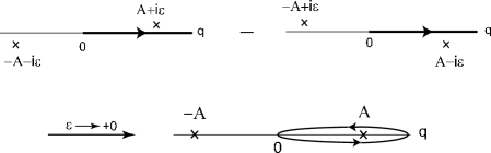
Figure 4: The contour of momentum $q_{E}$

The integration over $q_{E}$ for the second term (27) can be computed similarly. After integrating over the angular variables of $q_{E}$, we get

$$\begin{split}\mathcal{M}_{2}=\frac{g^{2}}{72\pi^{2}}\int_{0}^{\infty}dq_{E}\int_{0}^{1}dxe^{-2\alpha p_{E}^{2}(1-x)^{2}}&e^{-2\alpha q_{E}^{2}}q_{E}^{2}\frac{e^{4\alpha(1-x)p_{E}q_{E}}-e^{-4\alpha(1-x)p_{E}q_{E}}}{4\alpha(1-x)p_{E}q_{E}}\\ &\cdot\frac{1}{(q_{E}^{2}+p_{E}^{2}x(1-x)+m^{2}-i\epsilon)^{2}}.\end{split}$$

The imaginary part can be similarly expressed as a contour integration, and we obtain

$$\begin{split}2\mathrm{Im}\mathcal{M}_{2}=\frac{g^{2}}{36\pi}\int_{1/2-\gamma}^{1/2+\gamma}dx&\frac{e^{2\alpha p^{2}(1-x)^{2}}}{4\alpha(1-x)\sqrt{p^{2}}}\\ &\cdot\frac{e^{-2\alpha A^{2}}(-8\alpha A^{2}\sin B+2B\cos B)}{4A^{2}},\end{split}$$ (36)

where $B=4\alpha(1-x)\sqrt{p^{2}}A$.

The other terms can be also computed similarly. The term (28) becomes

$$\begin{split}2\mathrm{Im}\mathcal{M}_{3}=\frac{g^{2}}{36\pi}\int_{1/2-\gamma}^{1/2+\gamma}dx&\frac{e^{2\alpha p^{2}x^{2}}}{4\alpha x\sqrt{p^{2}}}\\ &\cdot\frac{e^{-2\alpha A^{2}}(-8\alpha A^{2}\sin C+2C\cos C)}{4A^{2}},\end{split}$$ (37)

where $C=4\alpha x\sqrt{p^{2}}A$. The term (29) becomes

$$\begin{split}2\mathrm{Im}\mathcal{M}_{4}=\frac{2g^{2}e^{\alpha p^{2}}}{36\pi}\int_{1/2-\gamma}^{1/2+\gamma}dx&\frac{e^{\alpha p^{2}(1-x)^{2}}}{2\alpha(1-x)\sqrt{p^{2}}}\\ &\cdot\frac{e^{-\alpha A^{2}}(-4\alpha A^{2}\sin(B/2)+B\cos(B/2))}{4A^{2}}.\end{split}$$ (38)

The (30) becomes

$$\begin{split}2\mathrm{Im}\mathcal{M}_{5}=\frac{2g^{2}}{36\pi}\int_{1/2-\gamma}^{1/2+\gamma}dx&\frac{e^{\alpha p^{2}(2x^{2}-2x+1)}}{2\alpha(1-2x)\sqrt{p^{2}}}\\ &\cdot\frac{e^{-2\alpha A^{2}}(-8\alpha A^{2}\sin D+2D\cos D)}{4A^{2}},\end{split}$$ (39)

where $D=2\alpha(1-2x)\sqrt{p^{2}}A$. Finally the term (31) becomes

$$\begin{split}2\mathrm{Im}\mathcal{M}_{6}=\frac{2g^{2}e^{\alpha p^{2}}}{36\pi}\int_{1/2-\gamma}^{1/2+\gamma}dx&\frac{e^{\alpha p^{2}x^{2}}}{2\alpha x\sqrt{p^{2}}}\\ &\cdot\frac{e^{-\alpha A^{2}}(-4\alpha A^{2}\sin(C/2)+C\cos(C/2))}{4A^{2}}.\end{split}$$ (40)

Let us now integrate over $x$ for these results (36)-(40). We change the variable $x$ to an angular variable $\varphi$,

$$x=\frac{1}{2}-\gamma\cos\varphi,$$ (41)

where $0\leq\varphi\leq\pi$. Then $A$ can be expressed as

$$A=\sqrt{p^{2}}\,\gamma\sin\varphi.$$ (42)

The integration can be explicitly carried out by using the exponential integral function, which is defined by

$$\mathrm{Ei}(-z)=\int_{\infty}^{z}\frac{e^{-t}}{t}dt.$$ (43)

The results are

$$2\mathrm{Im}\mathcal{M}_{2} =\frac{ig^{2}e^{2m^{2}\alpha}}{72\cdot 2\sqrt{p^{2}}\pi}\left[\mathrm{Ei}(2p^{2}\alpha(\gamma^{2}+\gamma e^{-i\varphi}+\gamma^{2}e^{-2i\varphi}))-(\varphi\rightarrow-\varphi)\right]\bigg{|}_{0}^{\pi},$$ (44)

$$2\mathrm{Im}\mathcal{M}_{3} =\frac{ig^{2}e^{2m^{2}\alpha}}{72\cdot 2\sqrt{p^{2}}\pi}\left[\mathrm{Ei}(2p^{2}\alpha(\gamma^{2}-\gamma e^{-i\varphi}+\gamma^{2}e^{-2i\varphi}))-(\varphi\rightarrow-\varphi)\right]\bigg{|}_{0}^{\pi},$$ (45)

$$2\mathrm{Im}\mathcal{M}_{4} =\frac{2ig^{2}e^{\alpha(p^{2}+m^{2})}}{72\cdot 2\sqrt{p^{2}}\pi}\left[\mathrm{Ei}(p^{2}\alpha(\gamma^{2}+\gamma e^{-i\varphi}+\gamma^{2}e^{-2i\varphi}))-(\varphi\rightarrow-\varphi)\right]\bigg{|}_{0}^{\pi},$$ (46)

$$2\mathrm{Im}\mathcal{M}_{5} =-\frac{2ig^{2}e^{2m^{2}\alpha}}{72\cdot 2\sqrt{p^{2}}\pi}\left[\mathrm{Ei}(2p^{2}\alpha(1+e^{2i\varphi}))-(\varphi\rightarrow-\varphi)\right]\bigg{|}_{0}^{\pi},$$ (47)

$$2\mathrm{Im}\mathcal{M}_{6} =\frac{2ig^{2}e^{\alpha(p^{2}+m^{2})}}{72\cdot 2\sqrt{p^{2}}\pi}\left[\mathrm{Ei}(p^{2}\alpha(\gamma^{2}-\gamma e^{-i\varphi}+\gamma^{2}e^{-2i\varphi}))-(\varphi\rightarrow-\varphi)\right]\bigg{|}_{0}^{\pi}.$$ (48)

Let us first evaluate (44). We first note that

$$\left[\mathrm{Ei}(2p^{2}\alpha(\gamma^{2}+\gamma e^{-i\varphi}+\gamma^{2}e^{-2i\varphi}))-(\varphi\rightarrow-\varphi)\right]\bigg{|}_{0}^{\pi}=\mathrm{Ei}(2p^{2}\alpha(\gamma^{2}+\gamma e^{-i\varphi}+\gamma^{2}e^{-2i\varphi}))\bigg{|}_{-\pi}^{\pi}.$$ (49)

Let us consider

$$u=\gamma^{2}+\gamma e^{-i\varphi}+\gamma^{2}e^{-2i\varphi}$$ (50)

in the argument of the exponential integral function in (49). Since $0<\gamma\leq\frac{1}{2}$, the trajectory of $u$ in the complex plane for the interval $-\pi\leq\varphi\leq\pi$ is given by a closed contour going clockwise around the origin $u=0$, as shown in Figure 5. Since the exponential integral function has a cut stretching between $u=0$ and $u=\infty$, (49) can be evaluated from the difference of the values of the exponential integral function on distinct sheets. From the definition (43), we find

$$\mathrm{Ei}(2p^{2}\alpha(\gamma^{2}+\gamma e^{-i\varphi}+\gamma^{2}e^{-2i\varphi}))\bigg{|}_{-\pi}^{\pi}=-\oint dt\frac{e^{-t}}{t}=-2\pi i,$$ (51)

where the closed contour of $t$ goes counterclockwise around the origin. Thus (44) is evaluated as

$$2\mathrm{Im}\mathcal{M}_{2}=\frac{g^{2}e^{2m^{2}\alpha}}{72\sqrt{p^{2}}}.$$ (52)

Figure 5: The contours of $u$ for $\gamma=\frac{1}{4}$ (left) and $\gamma=\frac{1}{2}$ (right).

We can evaluate (45), (46), (48) in the same manner as above. The results are

$$2\mathrm{Im}\mathcal{M}_{3} =\frac{g^{2}e^{2m^{2}\alpha}}{72\sqrt{p^{2}}},$$ (53)

$$2\mathrm{Im}\mathcal{M}_{4} =\frac{2g^{2}e^{\alpha(p^{2}+m^{2})}}{72\sqrt{p^{2}}},$$ (54)

$$2\mathrm{Im}\mathcal{M}_{6} =\frac{2g^{2}e^{\alpha(p^{2}+m^{2})}}{72\sqrt{p^{2}}}.$$ (55)

The evaluation of (47) requires a little care, since the exponential integral function is singular at $\varphi=\pi/2$. This is not a physical singularity, since there is no corresponding singularity in the original integration (39). In fact, it is allowed to deform the integration contour of $\varphi$ apart from real values. Let us deform the path in the direction of positive imaginary values as in Figure 6. Let us consider $v_{1}=1+e^{2i\varphi}$ and $v_{2}=1+e^{-2i\varphi}$ in the argument of the first and second terms of (47), respectively. Then $v_{1}$ does not surround the origin, while $v_{2}$ surrounds the origin clockwise as in Figure 7. Thus (47) is evaluated as

$$2\mathrm{Im}\mathcal{M}_{5}=\frac{2g^{2}e^{2m^{2}\alpha}}{72\sqrt{p^{2}}}.$$ (56)

Figure 6: The integration contour of $\varphi$ is deformed in the direction of positive imaginary values.

Figure 7: The contours of $v_{1}$ (left) and $v_{2}$ (right).

Collecting all the contributions (35), (52)-(56), we obtain the imaginary part of $\mathcal{M}$ as

$$2\mathrm{Im}\mathcal{M} =\frac{g^{2}}{72\sqrt{p^{2}}}(e^{2\alpha p^{2}}+4e^{2m^{2}\alpha}+4e^{\alpha(p^{2}+m^{2})})$$

$$=\frac{g^{2}}{72\sqrt{p^{2}}}(e^{\alpha p^{2}}+2e^{\alpha m^{2}})^{2}.$$ (57)

On the other hand, the other side of the Cutkosky rule, $\sum|\mathcal{M}|^{2}$, is given by

$$\begin{split}\sum|\mathcal{M}|^{2}=&\frac{1}{2}\bigg{(}\frac{g}{3}\bigg{)}^{2}\int\frac{d^{D}q}{(2\pi)^{D}}\frac{d^{D}l}{(2\pi)^{D}}(e^{\alpha p^{2}}+e^{\alpha q^{2}}+e^{\alpha l^{2}})^{2}\\ &\cdot(2\pi)^{D}\delta^{D}(l+q-p)2\pi\delta(q^{2}-m^{2})2\pi\delta(l^{2}-m^{2}).\end{split}$$ (58)

Putting $D=3$ and considering the center-of-mass frame $p=(p,0,0)$, we get

$$\sum|\mathcal{M}|^{2} =\frac{g^{2}}{18}\frac{1}{2\pi}\int\frac{d^{2}q}{4(|\vec{q}|^{2}+m^{2})}\delta(2\sqrt{|\vec{q}|^{2}+m^{2}}-p)(e^{\alpha p^{2}}+2e^{\alpha m^{2}})^{2}$$

$$=\frac{g^{2}}{72\sqrt{p^{2}}}(e^{\alpha p^{2}}+2e^{\alpha m^{2}})^{2},$$ (59)

which agrees with (57). Thus we conclude that, in $D=3$, the commutative nonassociative field theory based on the product (3) satisfies the one-loop unitarity relation of Figure 3. We also have checked the unitarity in four dimensions in perturbation of $\alpha$, and have found that the unitarity is satisfied at least upto the seventh order of $\alpha$. See the Appendix for details.

3 Nonassociative $\phi^{3}$ theory: quartic case

In the previous section we find the one-loop unitarity is satisfied for the commutative nonassociative scalar field theory obtained from the product defined by (3). But the real part of the one-loop amplitude has an exponential divergence in Minkowski spacetime, which is not relevant to the one-loop unitarity but may harm the significance of the field theory considered. In this section, we will define an improved commutative nonassociative product, and will study the one-loop unitarity of the scalar field theory obtained from it. The price to pay for this change is the loss of exact computation: One of the one-loop contributions will be computed in perturbation of a nonassociative parameter $\alpha$. We will find that the one-loop unitarity holds at least to the order considered.

The new product is defined by changing the square of the differentials in (3) into quartic power:

$$\phi(x)\ast\phi(x)=e^{\alpha((\partial_{a}+\partial_{b})^{2})^{2}}\phi(x+a)\phi(x+b)|_{a=b=0}.$$ (60)

In the momentum representation, the new star product is given by

$$e^{ipx}\ast e^{iqx}=e^{-\alpha\left((p+q)^{2}\right)^{2}}e^{i(p+q)x},$$ (61)

where $\alpha>0$. It is easy to show that this product is commutative but nonassociative. It is obviously Poincaré invariant.

In the same way as in Section 2, we obtain the following Feynman rules,

$$\textrm{propagator}: ~{}\frac{i}{p^{2}-m^{2}+i\epsilon},$$ (62)

$$\textrm{three-point vertex}: ~{}\frac{-ig}{3}(e^{-\alpha(p^{2})^{2}}+e^{-\alpha(q^{2})^{2}}+e^{-\alpha(k^{2})^{2}}),$$ (63)

where $p,q,k$ are the external momenta.

As in the previous section, we will check the one-loop Cutkosky rule of Figure 3 in $D=3$. The one-loop amplitude is given by

$$i\mathcal{M} =\bigg{(}\frac{-ig}{3}\bigg{)}^{2}\frac{1}{2}\int\frac{d^{3}q}{(2\pi)^{3}}(e^{-\alpha p^{4}}+e^{-\alpha q^{4}}+e^{-\alpha(p+q)^{4}})^{2}$$

$$\ \ \cdot\frac{i}{q^{2}-m^{2}+i\epsilon}\frac{i}{(p+q)^{2}-m^{2}+i\epsilon}$$

$$=\frac{g^{2}}{18}\int\frac{d^{3}q}{(2\pi)^{3}}\int_{0}^{1}dx(e^{-\alpha p^{4}}+e^{-\alpha q^{4}}+e^{-\alpha(p+q)^{4}})^{2}$$

$$\ \ \cdot\frac{1}{((q+p(1-x))^{2}+p^{2}x(1-x)-m^{2}+i\epsilon)^{2}},$$ (64)

where $p^{4}$ is the abbreviation for $(p^{2})^{2}$. There occur no exponential divergences, and the integration is convergent. After shifting the momentum variable, $q\to q-p(1-x)$, we obtain

$$i\mathcal{M} =\frac{g^{2}}{18}\int\frac{d^{3}q}{(2\pi)^{3}}\int_{0}^{1}dx\left(e^{-\alpha p^{4}}+e^{-\alpha(q-p(1-x))^{4}}+e^{-\alpha(q+px)^{4}}\right)^{2}$$

$$\cdot\frac{1}{(q^{2}+p^{2}x(1-x)-m^{2}+i\epsilon)^{2}},$$ (65)

where the exponential factors can be expanded as

$$\big{(}e^{-\alpha p^{4}} +e^{-\alpha(q-p(1-x))^{4}}+e^{-\alpha(q+px)^{4}}\big{)}^{2}$$

$$=e^{-2\alpha p^{4}}+e^{-2\alpha(q-p(1-x))^{4}}+e^{-2\alpha(q+px)^{4}}$$

$$+2e^{-\alpha p^{4}-\alpha(q-p(1-x))^{4}}+2e^{-\alpha(q-p(1-x))^{4}-\alpha(q+px)^{4}}+2e^{-\alpha p^{4}-\alpha(q+px)^{4}}.$$ (66)

We will compute each contribution in the followings.

Since the first term in (66) does not contain the dependence on $q$, we obtain a result similar to (35),

$$2\mathrm{Im}\mathcal{M}_{1}=\frac{g^{2}e^{-2\alpha p^{4}}}{72\sqrt{p^{2}}}.$$ (67)

Next let us evaluate the second term in (66). Wick rotating the momenta $p,q$ to Euclidean ones $p_{E},q_{E}$, and integrating over the angular variables of $q_{E}$, we get

$$\mathcal{M}_{2}=\frac{g^{2}\sqrt{\pi}}{72\sqrt{2\alpha}}\int_{0}^{\infty}\frac{dq_{E}}{4\pi^{2}}\int_{0}^{1}dx~{}\frac{q_{E}}{T^{\prime}}\frac{\mathrm{Erf}(\sqrt{2\alpha}(q_{E}+T^{\prime})^{2})-\mathrm{Erf}(\sqrt{2\alpha}(q_{E}-T^{\prime})^{2})}{(q_{E}+A^{\prime}_{\epsilon})^{2}(q_{E}-A^{\prime}_{\epsilon})^{2}},$$ (68)

where $A^{\prime}_{\epsilon}=\sqrt{-p_{E}^{2}x(1-x)-m^{2}+i\epsilon}$, $T^{\prime}=p_{E}(1-x)$ with an abbreviation $p_{E}=\sqrt{p_{E}^{2}}$, and the definition of the error function $\mathrm{Erf}(z)$ is given by

$$\mathrm{Erf}(z)=\frac{2}{\sqrt{\pi}}\int_{0}^{z}e^{-t^{2}}dt.$$ (69)

The integration over $q_{E}$ in the evaluation of the imaginary part of $\mathcal{M}_{2}$ can be carried out in the same way as in the previous section. The integration can be rewritten as a contour integration around the pole, and the result is

$$2\mathrm{Im}\mathcal{M}_{2}=\frac{g^{2}}{72\cdot 2\pi i}\int_{1/2-\gamma}^{1/2+\gamma}dx \bigg{[}\frac{1}{T}(e^{-2\alpha(A+iT)^{4}}-e^{-2\alpha(A-iT)^{4}})$$

$$+\frac{i}{A}(e^{-2\alpha(A+iT)^{4}}+e^{-2\alpha(A-iT)^{4}})\bigg{]},$$ (70)

where the external momentum has been Wick rotated to the Minkowski one, and $\gamma=\sqrt{(p^{2}-4m^{2})/4p^{2}}$, $A=\sqrt{p^{2}x(1-x)-m^{2}}$, $T=p(1-x)$ with an abbreviation $p=\sqrt{p^{2}}$. As before, $p^{2}>4m^{2}$ or $0<\gamma\leq\frac{1}{2}$ for the imaginary part of the amplitude to exist. After the change of variable $x=1/2-\gamma\cos\varphi$, the four terms in (70) can be collected into a simpler expression,

$$2\mathrm{Im}\mathcal{M}_{2}=\frac{g^{2}}{72\cdot 2p\pi i}\int_{0}^{2\pi}d\varphi\ e^{-2\alpha(A+iT)^{4}}\frac{A+iT}{T},$$ (71)

where $A=p\gamma\sin\varphi$, $T=p/2+p\gamma\cos\varphi$. Since $A+iT=ip\gamma e^{-i\varphi}+ip/2$, we carry out further the change of variable $z=e^{-i\varphi}$, and get

$$2\mathrm{Im}\mathcal{M}_{2} =\frac{g^{2}}{72p\pi i}\oint_{C}dze^{-2\alpha(p/2+p\gamma z)^{4}}\frac{\gamma z+1/2}{z+\gamma z^{2}+\gamma}$$

$$=\frac{g^{2}}{72p\pi i}\oint_{C}dz\frac{e^{-2\alpha(p/2+p\gamma z)^{4}}(\gamma z+1/2)}{\gamma(z-\bar{\alpha})(z-\bar{\beta})},$$ (72)

where

$$\bar{\alpha} =\frac{-1+\sqrt{1-4\gamma^{2}}}{2\gamma},$$ (73)

$$\bar{\beta} =\frac{-1-\sqrt{1-4\gamma^{2}}}{2\gamma},$$ (74)

and $C$ is the counterclockwise circular path with unit radius from the origin. Since $0<\gamma\leq 1/2$, $|\bar{\alpha}|<1$ and $|\bar{\beta}|>1$, and $z=\bar{\alpha}$ is the only pole in the inside of the unit circle $C$. Evaluating the residue of the pole at $z=\bar{\alpha}$, we get

$$2\mathrm{Im}\mathcal{M}_{2}=\frac{g^{2}}{72p}e^{-2\alpha m^{4}}.$$ (75)

We can easily obtain the contributions from the other terms in (66) except the fifth term. For example, the third term becomes the same as the second one after the change of variables, $p\to-p$ and $1-x\to x$. The other contributions can be also computed in similar ways. Thus we get

$$2\mathrm{Im}\mathcal{M}_{3} =\frac{g^{2}}{72p}e^{-2\alpha m^{4}},$$ (76)

$$2\mathrm{Im}\mathcal{M}_{4} =\frac{g^{2}}{36p}e^{-\alpha(p^{4}+m^{4})},$$ (77)

$$2\mathrm{Im}\mathcal{M}_{6} =\frac{g^{2}}{36p}e^{-\alpha(p^{4}+m^{4})}.$$ (78)

Finally we evaluate the contribution from the fifth term in (66). Wick rotating the momenta $p,q$ to Euclidean ones $p_{E},q_{E}$, and carrying out the integration over the angular coordinates of $q_{E}$, we get

$$\mathcal{M}_{5} =\frac{g^{2}\sqrt{\pi}}{36p\alpha^{1/2}}\int_{0}^{\infty}\frac{q_{E}dq_{E}}{4\pi^{2}}\int_{0}^{1}dxe^{-\alpha\frac{(q_{E}^{2}+p_{E}^{2}x(1-x))^{2}}{(1-x)^{2}+x^{2}}}$$

$$\cdot\frac{1}{(q_{E}+A^{\prime}_{\epsilon})^{2}(q_{E}-A^{\prime}_{\epsilon})^{2}\sqrt{(1-x)^{2}+x^{2}}}$$

$$\cdot\bigg{[}\mathrm{Erf}\bigg{(}\frac{\alpha^{1/2}[(1-x)(q_{E}+p_{E}(1-x))^{2}-x(q_{E}-p_{E}x)^{2}]}{\sqrt{(1-x)^{2}+x^{2}}}\bigg{)}$$

$$-\mathrm{Erf}\bigg{(}\frac{\alpha^{1/2}[(1-x)(q_{E}-p_{E}(1-x))^{2}-x(q_{E}+p_{E}x)^{2}]}{\sqrt{(1-x)^{2}+x^{2}}}\bigg{)}\bigg{]}.$$ (79)

The evaluation of the imaginary part and the integration over $q_{E}$ can be carried out in the same manner as above, and we get

$$2\mathrm{Im}\mathcal{M}_{5} =\frac{g^{2}\sqrt{\pi}}{72\pi ip}\int_{1/2-\gamma}^{1/2+\gamma}dx\frac{1}{A}\bigg{[}\bigg{(}\frac{\sqrt{\alpha}m^{2}A}{((1-x)^{2}+x^{2})^{3/2}}\bigg{)}e^{-\frac{\alpha m^{4}}{(1-x)^{2}+x^{2}}}$$

$$\cdot\bigg{\{}\mathrm{Erf}\bigg{(}\frac{\alpha^{1/2}[(1-x)(A+ip(1-x))^{2}-x(A-ipx)^{2}]}{\sqrt{(1-x)^{2}+x^{2}}}\bigg{)}$$

$$-\mathrm{Erf}\bigg{(}\frac{\alpha^{1/2}[(1-x)(A-ip(1-x))^{2}-x(A+ipx)^{2}]}{\sqrt{(1-x)^{2}+x^{2}}}\bigg{)}\bigg{\}}$$

$$+e^{-\frac{\alpha m^{4}}{(1-x)^{2}+x^{2}}}\frac{1}{\sqrt{\pi}\sqrt{(1-x)^{2}+x^{2}}}$$

$$\bigg{(}\frac{(1-x)(A+ip(1-x))-x(A-ipx)}{\sqrt{(1-x)^{2}+x^{2}}}e^{-\frac{\alpha[(1-x)(A+ip(1-x))^{2}-x(A-ipx)^{2}]^{2}}{(1-x)^{2}+x^{2}}}$$

$$-\frac{(1-x)(A-ip(1-x))-x(A+ipx)}{\sqrt{(1-x)^{2}+x^{2}}}e^{-\frac{\alpha[(1-x)(A-ip(1-x))^{2}-x(A+ipx)^{2}]^{2}}{(1-x)^{2}+x^{2}}}\bigg{)}\bigg{]}.$$ (80)

Carrying out the change of variable $x=1/2-\cos{\varphi}$, we obtain a simpler expression,

$$2\mathrm{Im}\mathcal{M}_{5} =\frac{g^{2}\sqrt{\pi}}{72\pi ip^{2}}\int_{0}^{2\pi}d\varphi\frac{e^{\frac{-\alpha m^{4}}{1/2+2\gamma^{2}\cos^{2}{\varphi}}}}{\sqrt{1/2+2\gamma^{2}\cos^{2}{\varphi}}}$$

$$\bigg{[}\frac{\sqrt{\alpha}m^{2}p\gamma\sin{\varphi}}{1/2+2\gamma^{2}\cos^{2}{\varphi}}\mathrm{Erf}\bigg{(}\frac{\sqrt{\alpha}(T(A+ipT)^{2}-S(A-ipS)^{2})}{\sqrt{1/2+2\gamma^{2}\cos^{2}{\varphi}}}\bigg{)}$$

$$+\frac{T(A+ipT)-S(A-ipS)}{\sqrt{\pi}\sqrt{1/2+2\gamma^{2}\cos^{2}{\varphi}}}$$

$$\cdot\exp{\bigg{\{}-\frac{\alpha(T(A+ipT)^{2}-S(A-ipS)^{2})^{2}}{1/2+2\gamma^{2}\cos^{2}{\varphi}}\bigg{\}}}\bigg{]},$$ (81)

where

$$S =\frac{1}{2}-\gamma\cos{\varphi},$$ (82)

$$T =\frac{1}{2}+\gamma\cos{\varphi}.$$ (83)

We carry out further the change of variable $w=e^{-2i\varphi}$. Then the first term in (81) is obtained as

$$\frac{\sqrt{2\pi\alpha}g^{2}m^{2}\gamma}{36p} \oint_{C}\frac{dw}{2\pi i}~{}e^{\frac{-2\alpha m^{4}w}{w+\gamma^{2}(w+1)^{2}}}~{}\frac{w-1}{(w+\gamma^{2}(w+1)^{2})^{3/2}}$$

$$\cdot\mathrm{Erf}\bigg{(}\frac{-\sqrt{2\alpha}p^{2}\gamma(\gamma^{2}w^{2}+(\gamma^{2}+5/4)w+1/4)}{\sqrt{w+\gamma^{2}(w+1)^{2}}}\bigg{)},$$ (84)

while the second term is obtained as

$$\frac{g^{2}}{36p} \oint_{C}\frac{dw}{2\pi i}\frac{1+2\gamma^{2}(w+1)}{w+\gamma^{2}(w+1)^{2}}e^{-\frac{\alpha p^{4}}{8}(1+24\gamma^{2}w+16\gamma^{4}w^{2})}.$$ (85)

Here the contour $C$ denotes a counterclockwise circular path with unit radius from the origin. We have multiplied (84) and (85) by a factor of $2$, because $w$ goes around the origin twice when $\varphi$ varies from $0$ to $2\pi$.

The evaluation of the second contribution (85) is straightforward. When $\gamma$ is in the range $0<\gamma\leq\frac{1}{2}$, the only pole in the unit circle is at

$$w=\frac{-2\gamma^{2}-1+\sqrt{1+4\gamma^{2}}}{2\gamma^{2}}.$$ (86)

Evaluating the residue of the pole, we get

$$\frac{g^{2}}{36p}e^{-2\alpha m^{4}}e^{-2\alpha p^{2}m^{2}\big{(}-1+\sqrt{2-\frac{4m^{2}}{p^{2}}}~{}\big{)}}.$$ (87)

On the other hand, we have not succeeded in evaluating exactly the first contribution (84). We have computed the contribution in the perturbation of $\alpha$ as follows. The error function ${\rm Erf}(z)$ has a series representation,

$${\rm Erf}(z)=\frac{2}{\sqrt{\pi}}e^{-z^{2}}\sum_{k=0}^{\infty}\frac{2^{k}z^{2k+1}}{(2k+1)!!}.$$ (88)

Applying this formula to (84), we obtain

$$-\frac{\alpha g^{2}\gamma^{2}m^{2}p}{9}\oint_{C}\frac{dw}{2\pi i} \frac{(w-1)(\gamma^{2}w^{2}+(\gamma^{2}+5/4)w+1/4)}{(w+\gamma^{2}(w+1)^{2})^{2}}e^{-\frac{\alpha p^{4}}{8}(1+24\gamma^{2}w+16\gamma^{4}w^{2})}$$

$$\cdot\sum_{k=0}^{\infty}\frac{1}{(2k+1)!!}\left[\frac{4\alpha p^{4}\gamma^{2}(\gamma^{2}w^{2}+(\gamma^{2}+5/4)w+1/4)^{2}}{w+\gamma^{2}(w+1)^{2}}\right]^{k}.$$ (89)

In the unit circle $C$, there is only one pole at (86). Since the order of the pole becomes higher in higher order terms of the series, it seems hard to obtain an exact result from the expression (89). On the other hand, the series in (89) can be regarded as a perturbative expansion in $\alpha$. Using Mathematica, we have computed (89) in perturbation of $\alpha$ upto the seventh order, and have found that (89) actually agrees with the expansion of

$$\frac{g^{2}}{36p}e^{-2\alpha m^{4}}\left[1-e^{-2\alpha p^{2}m^{2}\left(-1+\sqrt{2-\frac{4m^{2}}{p^{2}}}~{}\right)}\right].$$ (90)

Thus if we assume this is correct in all orders of $\alpha$, adding (87) and (90), we finally obtain

$$2\mathrm{Im}\mathcal{M}_{5}=\frac{g^{2}}{36p}e^{-2\alpha m^{4}}.$$ (91)

Collecting all the contributions, (67), (75)-(78), (91), the imaginary part of the amplitude is obtained as

$$2\mathrm{Im}\mathcal{M} =\frac{g^{2}}{72p}\left(e^{-2\alpha p^{4}}+4e^{-2\alpha m^{4}}+4e^{-2\alpha(p^{4}+m^{4})}\right)$$

$$=\frac{g^{2}}{72p}\left(e^{-\alpha p^{4}}+2e^{-\alpha m^{4}}\right)^{2}.$$ (92)

The other side of the Cutkosky rule, $\sum|\mathcal{M}|^{2}$, can be computed in the similar manner as in the preceding section, and we obtain

$$\sum|\mathcal{M}|^{2}=\frac{g^{2}}{72p}\left(e^{-\alpha p^{4}}+2e^{-\alpha m^{4}}\right)^{2},$$ (93)

which agrees with (92). Thus the scalar field theory obtained from the star product (60) satisfies the one-loop unitarity of Figure 3.

4 Field theories on Poincaré invariant commutative associative spacetimes

In this section, we will consider scalar field theories obtained from Poincaré invariant commutative associative algebras. It will be shown that momentum dependence of couplings does not appear in such cases. Therefore an algebra must violate commutativity or associativity for scalar field theory to have non-trivial properties. This would be a physical restatement of the mathematical Gelfand-Naimark theorem, which asserts that any associative commutative algebra is canonically isomorphic to the algebra of functions on some space with the usual pointwise multiplication.

A Poincaré invariant commutative associative algebra has the general expression,

$$e^{ip_{1}x}\ast e^{ip_{2}x}=f(p_{1},p_{2})e^{i(p_{1}+p_{2})x},$$ (94)

where $f(p_{1},p_{2})$ is a Lorentz invariant function of two momenta $p_{1},p_{2}$ and must satisfy the conditions,

$$f(p_{1},p_{2}) =f(p_{2},p_{1}),$$ (95)

$$f(p_{1},p_{2})f(p_{1}+p_{2},p_{3}) =f(p_{1},p_{2}+p_{3})f(p_{2},p_{3}),$$ (96)

where (95) and (96) are the conditions for commutativity and associativity, respectively. We also assume a positivity property,

$$f(p,-p)>0$$ (97)

for general $p$. As can be seen below, this condition is required for the kinetic term of field theory to be non-singular.

Let us consider scalar $\phi^{3}$ theory based on the above star product. The action is given by

$$S=\int d^{D}x\bigg{[}\frac{1}{2}\partial_{\mu}\phi(x)\ast\partial^{\mu}\phi(x)-\frac{1}{2}m^{2}\phi(x)\ast\phi(x)-\frac{g}{3!}\phi(x)\ast\phi(x)\ast\phi(x)\bigg{]}.$$ (98)

We define the Fourier transformation of $\phi(x)$ as

$$\phi(x)=\int\frac{d^{D}p}{(2\pi)^{D}}N(p)\tilde{\phi}(p)e^{-ipx},$$ (99)

where $N(p)$ is a normalization factor, which will be determined later. Substituting the Fourier transformation to the action, we get

$$S =\int_{p}\frac{1}{2}N(p)N(-p)f(p,-p)(p^{2}-m^{2})\tilde{\phi}(p)\tilde{\phi}(-p)$$

$$-\frac{g}{3!}\int_{p}\int_{q}\int_{k}N(p)N(q)N(k)f(p,q)f(p+q,k)\delta^{D}(p+q+k)\tilde{\phi}(p)\tilde{\phi}(q)\tilde{\phi}(k),$$ (100)

where $\int_{p}$ is $\int d^{D}p/(2\pi)^{D}$.

The physics should not depend on the normalization $N(p)$ of the momentum modes. Therefore we can make the propagator of this theory to have the usual form $i/(p^{2}-m^{2}+i\epsilon)$ by choosing

$$N(p)=\frac{1}{\sqrt{f(p,-p)}}.$$ (101)

This choice is allowed from the positivity assumption (97). Then the momentum dependence of the three-point vertex is obtained as

$$\frac{f(p,q)f(p+q,-p-q)}{\sqrt{f(p,-p)}\sqrt{f(q,-q)}\sqrt{f(-p-q,p+q)}}.$$ (102)

For the convenience of the following discussions, let us consider the square of (102),

$$h=\frac{f^{2}(p,q)f(p+q,-p-q)}{f(p,-p)f(q,-q)}.$$ (103)

Using the associativity (96), $f(p,q)f(p+q,-p-q)=f(p,-p)f(q,-p-q)$, $h$ can be rewritten as

$$h=\frac{f(p,q)f(q,-p-q)}{f(q,-q)}.$$ (104)

Since $f(p,q)$ is a Lorentz invariant function, it has the property,

$$f(p,-q)=f(-p,q).$$ (105)

Using (95), (96), (104) and (105), we can further show

$$h=f(p,0).$$ (106)

On the other hand, from (96), we find $f(p,-p)f(0,0)=f(p,-p)f(-p,0)$. Using the positivity (97), we conclude

$$h=f(0,0).$$ (107)

Therefore $h$ is actually a constant, and the coupling does not have momentum dependence.

The above proof can be generalized to the general coupling $(\ast\phi)^{n+1}$ as follows. The corresponding generalization of $h$ is given by

$$h_{n}=\frac{f\left(\sum_{j=1}^{n}p_{j},-\sum_{j=1}^{n}p_{j}\right)\prod_{i=1}^{n-1}f^{2}\left(\sum_{j=1}^{i}p_{j},p_{i+1}\right)}{\prod_{i=1}^{n}f\left(p_{i},-p_{i}\right)}.$$ (108)

This quantity satisfies an inductive relation,

$$h_{n}=\frac{f^{2}(q,p_{n})f(q+p_{n},-q-p_{n})}{f(q,-q)f(p_{n},-p_{n})}h_{n-1},$$ (109)

where $q=\sum_{i=1}^{n-1}p_{i}$. The factor in front has actually the same form as (103). Therefore $h_{n}$ and $h_{n-1}$ are related by a constant multiplication. Since we have shown $h_{2}$ is a constant, any $h_{n}$ is also a constant by induction. Thus we see that commutative associative scalar field theories do not have momentum dependence of couplings.

5 Discussions and comments

We find that our commutative nonassociative field theories satisfy the one-loop unitarity of Figure 3 in the standard path integral scheme. This is in contrast with the violation of unitarity in noncommutative field theories with space/time noncommutativity in the standard path integral scheme. However, our result is based on the explicit computations of the one-loop self-energy diagrams of the field theories obtained from certain commutative nonassociative algebras. Therefore it is not clear how general our result is, i.e. whether unitarity holds for other diagrams and other commutative nonassociative algebras. Concerning this question, we point out a qualitative difference in non-locality between our field theories and the noncommutative field theories in the following paragraph.

Noncommutative field theories defined by Moyal product (1) are non-local in real directions. We can easily see this by using the momentum representation as

$$e^{ipx}\ast e^{iqx} =e^{-\frac{i}{2}p_{\mu}\theta^{\mu\nu}q_{\nu}}e^{i(p+q)x}$$

$$=e^{ip_{\mu}(x^{\mu}-\frac{1}{4}\theta^{\mu\nu}q_{\nu})}e^{iq_{\mu}(x^{\mu}+\frac{1}{4}\theta^{\mu\nu}p_{\nu})}.$$ (110)

Therefore when there is space/time noncommutativity, there exists non-locality in time, and field theories will inevitably show some pathological behaviors such as violation of unitarity [24]-[26]. On the other hand, our star product (4) can be rewritten in the form,

$$e^{ipx}\ast e^{iqx} =e^{\alpha(p+q)^{2}}e^{i(p+q)x}$$

$$=e^{ip\cdot(x-i\alpha(p+q))}e^{iq\cdot(x-i\alpha(p+q))}.$$ (111)

One notices that the coordinates are shifted in the imaginary directions. This feature is also true for the star product (61). Therefore our star products do not have the non-locality in the real time direction, and this qualitative difference may be the essence of why our field theories do not show the violation of unitarity, even though our products contain an infinite number of derivatives with respect to the coordinates.

It is known that noncommutative field theories have the UV-IR mixing property [16]-[18]. The UV-IR mixing is a phenomenon that the ultra-violet divergences appear when external momenta approach zero. This occurs because the limit of vanishing external momenta has similar effects as the commutative limit $\theta^{\mu\nu}\to 0$ in loop amplitudes. On the other hand, the explicit expressions of the one-loop amplitudes (24), (64) do not seem to have this sort of similarity between the two limits. Therefore our commutative nonassociative field theories will be free from the UV/IR mixing.

The idea of noncommutativity of coordinates stems from the quantization of spacetime. But how about nonassociativity? Is there any relation to quantization? Actually, it seems that nonassociativity can lead to noncommutativity in some situations. Let us define a right-operation $R(a)$ for an element $a$ of a nonassociative algebra as

$$R(a)b\equiv a*b.$$ (112)

Then one finds

$$[R(a),R(b)]c=a*(b*c)-b*(a*c),$$ (113)

which does not vanish in general even when the nonassociative algebra is commutative. Therefore $R(a)$ is noncommutative in general. It would be interesting to find such effects of noncommutativity in commutative nonassociative field theories.

Appendix A Unitarity in four dimensions

In this section, we check the unitarity in four dimensions in perturbation of $\alpha$.

Let us consider the quadratic case (3). From (25), the amplitude is given by

$$\mathcal{M} =\frac{g^{2}}{18}\int\frac{d^{4}q_{E}}{(2\pi)^{4}}\int_{0}^{1}dx\big{(}e^{-2\alpha p_{E}^{2}}+e^{-2\alpha(q_{E}-p_{E}x)^{2}}+e^{-2\alpha(q_{E}+p_{E}x)^{2}}$$

$$+2e^{-\alpha p_{E}^{2}}(e^{-\alpha(q_{E}-p_{E}x)^{2}}+e^{-\alpha(q_{E}+p_{E}x)^{2}})+2e^{-\alpha(q_{E}-p_{E}(1-x))^{2}}e^{-\alpha(q_{E}+p_{E}x)^{2}}\big{)}$$

$$\cdot\frac{1}{(q_{E}^{2}+p_{E}^{2}x(1-x)+m^{2}-i\epsilon)^{2}}.$$

Parameterizing the four-momentum $q_{E}$ with the radial and the spherical coordinates, it becomes

$$\mathcal{M} =\frac{g^{2}}{18(2\pi)^{4}}\int_{0}^{\infty}dq_{E}q_{E}^{3}\int_{0}^{2\pi}d\omega\int_{0}^{\pi}d\varphi\sin{\varphi}\int_{0}^{\pi}d\theta\sin^{2}{\theta}\int_{0}^{1}dx$$

$$\big{(}e^{-2\alpha p_{E}^{2}}+e^{-2\alpha(q_{E}^{2}+p_{E}^{2}x^{2})}(e^{4\alpha q_{E}p_{E}x\cos{\theta}}+e^{-4\alpha q_{E}p_{E}x\cos{\theta}})$$

$$+2e^{-\alpha p_{E}^{2}}e^{-\alpha(q_{E}^{2}+p_{E}^{2}x^{2})}(e^{2\alpha q_{E}p_{E}x\cos{\theta}}+e^{-2\alpha q_{E}p_{E}x\cos{\theta}})$$

$$+2e^{-\alpha(2q_{E}^{2}+p_{E}^{2}(2x^{2}-2x+1)-2p_{E}q_{E}(1-2x)\cos{\theta})}\big{)}\frac{1}{(q_{E}^{2}+p_{E}^{2}x(1-x)+m^{2}-i\epsilon)^{2}}$$

$$=\frac{4\pi g^{2}}{18(2\pi)^{4}}\int_{0}^{\infty}dq_{E}q_{E}^{3}\int_{-1}^{1}dt\sqrt{1-t^{2}}\int_{0}^{1}dx$$

$$(e^{-2\alpha p_{E}^{2}}$$ (114)

$$+2e^{-2\alpha(q_{E}^{2}+p_{E}^{2}x^{2})}\cosh{(4\alpha q_{E}p_{E}xt)}$$ (115)

$$+4e^{-\alpha p_{E}^{2}}e^{-\alpha(q_{E}^{2}+p_{E}^{2}x^{2})}\cosh{(2\alpha q_{E}p_{E}xt)}$$ (116)

$$+2e^{-\alpha(2q_{E}^{2}+p_{E}^{2}(2x^{2}-2x+1)-2p_{E}q_{E}(1-2x)t)})$$ (117)

$$\cdot\frac{1}{(q_{E}^{2}+p_{E}^{2}x(1-x)+m^{2}-i\epsilon)^{2}}.$$

Let us calculate the first term (114). After integrating over the variable $t$ and carrying out the replacement $p_{E}^{2}=-p^{2}$, we obtain

$$\mathcal{M}_{1}=\frac{g^{2}}{144\pi^{2}}e^{2\alpha p^{2}}\int_{0}^{\infty}dq_{E}\int_{0}^{1}dx\frac{q_{E}^{3}}{(q_{E}^{2}-p^{2}x(1-x)+m^{2}-i\epsilon)^{2}}.$$ (118)

We can evaluate the imaginary part as we have done in section 2. After carrying out the contour integration over $q_{E}$, we obtain

$$2\mathrm{Im}\mathcal{M}_{1} =\frac{g^{2}}{144\pi}e^{2\alpha p^{2}}\int_{1/2-\gamma}^{1/2+\gamma}dx$$

$$=\frac{g^{2}}{72\pi}e^{2\alpha p^{2}}\sqrt{\frac{p^{2}-4m^{2}}{4p^{2}}}.$$ (119)

This first order in $\alpha$ is

$$2\mathrm{Im}\mathcal{M}_{1}^{(1)}=\frac{g^{2}}{36\pi}\alpha p^{2}\sqrt{\frac{p^{2}-4m^{2}}{4p^{2}}}.$$ (120)

Next let us calculate the second term (115). After integrating over the variable $t$ and carrying out the replacement $p_{E}^{2}=-p^{2}$, we obtain

$$\mathcal{M}_{2} =\frac{g^{2}}{36\pi^{2}}\int_{0}^{\infty}dq_{E}\int_{0}^{1}dxq_{E}^{3}e^{-2\alpha(q_{E}^{2}-p^{2}x^{2})}J_{1}(4\alpha\sqrt{p^{2}}q_{E}x)$$

$$\cdot\frac{1}{4\alpha\sqrt{p^{2}}q_{E}x(q_{E}+A_{\epsilon})^{2}(q_{E}-A_{\epsilon})^{2}},$$ (121)

where $J_{\nu}(z)$ is the Bessel function.

To obtain the imaginary part, we evaluate

$$2\mathrm{Im}\mathcal{M}_{2} =\frac{g^{2}}{36\pi^{2}i}\oint dq_{E}\int_{1/2-\gamma}^{1/2+\gamma}dxq_{E}^{3}e^{-2\alpha(q_{E}^{2}-p^{2}x^{2})}J_{1}(4\alpha\sqrt{p^{2}}q_{E}x)$$

$$\cdot\frac{1}{4\alpha\sqrt{p^{2}}q_{E}x(q_{E}+A+i\epsilon)^{2}(q_{E}-A-i\epsilon)^{2}},$$ (122)

where the contour is given by Figure 4.

After carrying out the contour integration over $q_{E}$, we obtain

$$2\mathrm{Im}\mathcal{M}_{2}=\frac{g^{2}}{18\pi}\int_{1/2-\gamma}^{1/2+\gamma}dx\frac{1}{4}e^{-2\alpha(A^{2}-p^{2}x^{2})}\bigg{(}(1-2\alpha A^{2})\frac{J_{1}(4\alpha\sqrt{p^{2}}Ax)}{2\alpha\sqrt{p^{2}}Ax}-J_{2}(4\alpha\sqrt{p^{2}}Ax)\bigg{)}.$$ (123)

Carrying out Taylor expansion in $\alpha$, the first order in $\alpha$ is

$$2\mathrm{Im}\mathcal{M}_{2}^{(1)} =\frac{g^{2}\alpha}{18\pi}\int_{1/2-\gamma}^{1/2+\gamma}dx\left(m^{2}+\frac{1}{2}p^{2}x(-2+3x)\right)$$

$$=\frac{g^{2}\alpha m^{2}}{18\pi}\sqrt{\frac{p^{2}-4m^{2}}{4p^{2}}}.$$ (124)

In the same way, the third term (116) is

$$2\mathrm{Im}\mathcal{M}_{3}^{(1)}=\frac{g^{2}\alpha}{18\pi}(p^{2}+m^{2})\sqrt{\frac{p^{2}-4m^{2}}{4p^{2}}}.$$ (125)

Finally let us evaluate the forth term (117). After integrating over the variable $t$ and carrying out the replacement $p_{E}^{2}=-p^{2}$, we obtain

$$\mathcal{M}_{4}=\frac{g^{2}}{36\pi^{2}}\int_{0}^{\infty}dq_{E}\int_{0}^{1}dxq_{E}^{3}e^{-\alpha(2q_{E}^{2}-p^{2}(2x^{2}-2x+1))}\frac{J_{1}(2\alpha\sqrt{p^{2}}q_{E}(1-2x))}{2\alpha\sqrt{p^{2}}q_{E}(1-2x)(q_{E}+A_{\epsilon})^{2}(q_{E}-A_{\epsilon})^{2}}.$$ (126)

To obtain the imaginary part, we evaluate

$$2\mathrm{Im}\mathcal{M}_{4} =\frac{g^{2}}{36\pi^{2}i}\oint dq_{E}\int_{1/2-\gamma}^{1/2+\gamma}dxq_{E}^{3}e^{-\alpha(2q_{E}^{2}-p^{2}(2x^{2}-2x+1))}$$

$$\cdot\frac{J_{1}(2\alpha\sqrt{p^{2}}q_{E}(1-2x))}{2\alpha\sqrt{p^{2}}q_{E}(1-2x)(q_{E}+A+i\epsilon)^{2}(q_{E}-A-i\epsilon)^{2}}.$$ (127)

After carrying out the contour integration over $q_{E}$, we obtain

$$2\mathrm{Im}\mathcal{M}_{4} =\frac{g^{2}}{18\pi}\int_{1/2-\gamma}^{1/2+\gamma}dx\frac{1}{4}e^{-\alpha(2A^{2}+p^{2}(-1+2x-2x^{2}))}$$

$$\cdot\bigg{(}(1-2\alpha A^{2})\frac{J_{1}(2\alpha\sqrt{p^{2}}A(1-2x))}{\alpha\sqrt{p^{2}}A(1-2x)}-J_{2}(2\alpha\sqrt{p^{2}}A(1-2x))\bigg{)}.$$ (128)

Carrying out Taylor expansion in $\alpha$, the first order in $\alpha$ is

$$2\mathrm{Im}\mathcal{M}_{4}^{(1)} =\frac{g^{2}\alpha}{18\pi}\int_{1/2-\gamma}^{1/2+\gamma}dx\frac{1}{4}(4m^{2}+p^{2}(1-6x+6x^{2}))$$

$$=\frac{g^{2}\alpha}{18\pi}m^{2}\sqrt{\frac{p^{2}-4m^{2}}{4p^{2}}}.$$ (129)

Thus, collecting the results (120), (A), (125) and (A), the imaginary part of the amplitude in the first order of $\alpha$ is

$$2\mathrm{Im}\mathcal{M}=\frac{\alpha g^{2}}{12\pi}(p^{2}+2m^{2})\sqrt{\frac{p^{2}-4m^{2}}{4p^{2}}}.$$ (130)

On the other hand, the other side of the Cutkosky rule, $\Sigma|\mathcal{M}|^{2}$ is given by

$$\Sigma|\mathcal{M}|^{2} =\frac{1}{2}\left(\frac{g}{3}\right)^{2}\int\frac{d^{4}q}{(2\pi)^{4}}\frac{d^{4}l}{(2\pi)^{4}}(e^{\alpha p^{2}}+e^{\alpha q^{2}}+e^{\alpha l^{2}})^{2}$$

$$\cdot(2\pi)^{4}\delta^{4}(l+q-p)2\pi\delta(q^{2}-m^{2})2\pi\delta(l^{2}-m^{2})$$

$$=\frac{g^{2}}{18(2\pi)^{2}}(e^{\alpha p^{2}}+2e^{\alpha m^{2}})^{2}\int\frac{d^{3}q}{2\sqrt{\vec{q}^{2}+m^{2}}}\int\frac{d^{3}l}{2\sqrt{\vec{l}^{2}+m^{2}}}\delta^{4}(l+q-p)$$

$$=\frac{g^{2}}{72\pi}\sqrt{\frac{p^{2}-4m^{2}}{4p^{2}}}(e^{\alpha p^{2}}+2e^{\alpha m^{2}})^{2}.$$ (131)

The first order of $\alpha$ of $\Sigma|\mathcal{M}|^{2}$ is

$$\Sigma|\mathcal{M}|^{2(1)}=\frac{g^{2}\alpha}{12\pi}\sqrt{\frac{p^{2}-4m^{2}}{4p^{2}}}(p^{2}+2m^{2}).$$ (132)

Thus we find that the unitarity is satisfied in the first order of $\alpha$ in four dimensions. We can check the unitarity in higher orders of $\alpha$ in the same way, and have found that the unitarity is satisfied at least up to the seventh order of $\alpha$, using the Mathematica.

References

[1]H. S. Snyder,
“Quantized Space-Time,”
Phys. Rev. 71, 38 (1947).
[2]
C. N. Yang,
“On Quantized Space-Time,”
Phys. Rev. 72, 874 (1947).
[3]
A. Connes and J. Lott,
“Particle Models And Noncommutative Geometry (Expanded Version),”
Nucl. Phys. Proc. Suppl. 18B, 29 (1991).
[4]
S. Doplicher, K. Fredenhagen and J. E. Roberts,
“The Quantum structure of space-time at the Planck scale and quantum fields,”
Commun. Math. Phys. 172, 187 (1995)
[arXiv:hep-th/0303037].
[6]
N. Seiberg and E. Witten,
“String theory and noncommutative geometry,”
JHEP 9909, 032 (1999)
[arXiv:hep-th/9908142].
[7]
L. Freidel and E. R. Livine,
“Ponzano-Regge model revisited. III: Feynman diagrams and effective field
theory,”
Class. Quant. Grav. 23, 2021 (2006)
[arXiv:hep-th/0502106].
[8]
M. Chaichian, P. P. Kulish, K. Nishijima and A. Tureanu,
“On a Lorentz-invariant interpretation of noncommutative space-time and its
implications on noncommutative QFT,”
Phys. Lett. B 604, 98 (2004)
[arXiv:hep-th/0408069].
[9]
M. Chaichian, P. Presnajder and A. Tureanu,
“New concept of relativistic invariance in NC space-time: Twisted Poincare
symmetry and its implications,”
Phys. Rev. Lett. 94, 151602 (2005)
[arXiv:hep-th/0409096].
[10]
J. Gomis and T. Mehen,
“Space-time noncommutative field theories and unitarity,”
Nucl. Phys. B 591, 265 (2000)
[arXiv:hep-th/0005129].
[11]
L. Alvarez-Gaume, J. L. F. Barbon and R. Zwicky,
“Remarks on time-space noncommutative field theories,”
JHEP 0105, 057 (2001)
[arXiv:hep-th/0103069].
[12]
C. S. Chu, J. Lukierski and W. J. Zakrzewski,
“Hermitian analyticity, IR/UV mixing and unitarity of noncommutative field
theories,”
Nucl. Phys. B 632, 219 (2002)
[arXiv:hep-th/0201144].
[13]
D. Bahns, S. Doplicher, K. Fredenhagen and G. Piacitelli,
“On the unitarity problem in space/time noncommutative theories,”
Phys. Lett. B 533, 178 (2002)
[arXiv:hep-th/0201222].
[14]
C. h. Rim and J. H. Yee,
“Unitarity in space-time noncommutative field theories,”
Phys. Lett. B 574, 111 (2003)
[arXiv:hep-th/0205193].
[15]
N. Seiberg, L. Susskind and N. Toumbas,
“Space/time non-commutativity and causality,”
JHEP 0006, 044 (2000)
[arXiv:hep-th/0005015].
[16]
T. Filk,
“Divergencies in a field theory on quantum space,”
Phys. Lett. B 376, 53 (1996).
[17]
S. Minwalla, M. Van Raamsdonk and N. Seiberg,
“Noncommutative perturbative dynamics,”
JHEP 0002, 020 (2000)
[arXiv:hep-th/9912072].
[18]
M. Hayakawa,
“Perturbative analysis on infrared aspects of noncommutative QED on R**4,”
Phys. Lett. B 478, 394 (2000)
[arXiv:hep-th/9912094].
[19]
L. Cornalba and R. Schiappa,
“Nonassociative star product deformations for D-brane worldvolumes in curved
backgrounds,”
Commun. Math. Phys. 225, 33 (2002)
[arXiv:hep-th/0101219].
[20]
E. Witten,
“Noncommutative Geometry And String Field Theory,”
Nucl. Phys. B 268, 253 (1986).
[21]
T. Ootsuka, E. Tanaka and E. Loginov,
“Non-associative gauge theory,”
arXiv:hep-th/0512349.
[22]
S. Majid,
“Gauge theory on nonassociative spaces,”
J. Math. Phys. 46, 103519 (2005)
[arXiv:math.qa/0506453].
[23]
P. de Medeiros and S. Ramgoolam,
“Non-associative gauge theory and higher spin interactions,”
JHEP 0503, 072 (2005)
[arXiv:hep-th/0412027].
[24]
K. Fujikawa,
“Path integral for space-time noncommutative field theory,”
Phys. Rev. D 70, 085006 (2004)
[arXiv:hep-th/0406128].
[25]
C. Hayashi, “Hamiltonian Formalism in Non-local Field Theories,”
Prog. Theor. Phys. 10 (1953), 533.
[26]
S. Tanaka,
“Unitarity Problem In Nonlocal Field Theories: Some Remarks On String Field
Theory,”
Prog. Theor. Phys. 80, 566 (1988).