Lorentz Violating Inflation

Abstract

We explore the impact of Lorentz violation on the inflationary scenario. More precisely, we study the inflationary scenario in the scalar-vector-tensor theory where the vector is constrained to be unit and time like. It turns out that the Lorentz violating vector affects the dynamics of the chaotic inflationary model and divides the inflationary stage into two parts; the Lorentz violating stage and the standard slow roll stage. We show that the universe is expanding as an exact de Sitter spacetime in the Lorentz violating stage although the inflaton field is rolling down the potential. Much more interestingly, we find exact Lorentz violating inflationary solutions in the absence of the inflaton potential. In this case, the inflation is completely associated with the Lorentz violation. We also mention some consequences of Lorentz violating inflation which can be tested by observations.

I Introduction

The Lorentz invariance has been considered as the most fundamental symmetry of physics. However, as far as we know, any symmetry is not realized exactly or spontaneously broken. Hence, it is important to investigate a possibility of violation of Lorentz invariance. In fact, the observation of high energy cosmic rays reports super GZK events though it needs further confirmation Greisen ; Zatsepin:1966jv ; Takeda:1998ps . This may suggests the Lorentz violation Sato:2000vu ; Coleman:1998ti . Theoretically, any quantum theory of gravity requires drastic modification of the picture of space-time at the Planck scale Amelino-Camelia:1997gz . Some of them yields the Lorentz violation Kostelecky:1988zi .

The impact of Lorentz violation on physics should be broad. Even in the cosmology, there are many subjects which should be reconsidered. For example, the dark matter and the dark energy problem, the inflation, the baryogenesis, cosmic rays, and so on Bekenstein:2004ne ; Carroll:2004ai ; Carroll:2005dj . Here, we shall concentrate on the inflationary scenario.

Typically, the Lorentz violation yields the preferred frame. In the case of the standard model of particles, there are strong constraints on the existence of the preferred frame Mattingly:2005re . In contrast, there is no reason to refuse the preferred frame in cosmology. Rather, there is a natural preferred frame which is defined by cosmic microwave background radiation (CMB). Therefore, there is room to consider the gravitational theory which allows the preferred frame. The purpose of this paper is to clarify what occurs in inflationary stage when we allow the preferred frame from the beginning. It turns out that there is a chance to detect the evidence of the Lorentz violation through the observation of the cosmic microwave background radiation and the primordial gravitational waves.

When we talk about the Lorentz violation, we have to specify the model somehow. Recently, various types of theory of gravity with the Lorentz violation are proposed. One is the ghost condensation model which has a non-conventional kinetic term. In the stable vacuum, the kinetic term has the expectation value. Hence, the Lorentz invariance is violated spontaneously Arkani-Hamed:2003uy ; Arkani-Hamed:2004ar ; Cheng:2006us . This violation mechanism is an interesting possibility. The inflationary scenario in the ghost condensation was also investigated in this context Arkani-Hamed:2003uz . Another interesting one is brane model Csaki:2000dm ; Cline:2003xy ; Libanov:2005nv . From the string theoretical point of view, the braneworld picture seems to be natural. Hence, it is important to examine the Lorentz violation in the braneworld. Of course, there are other interesting models.

In this paper, we will consider the spontaneous breaking of Lorentz symmetry due to a vector field Gripaios:2004ms . When this vector field couples to the gravity, we obtain the Lorentz violating theory of gravity, the so-called Einstein-Ather theory Jacobson:2000xp . Interestingly, this theory has a wide parameter region where all of current experiments and observations can be explained Eling:2003rd ; Graesser:2005bg ; Foster:2005dk ; Foster:2006az . When we consider the cosmology, parameters could depend on time. The time evolution of parameters can be regarded as a consequence of the dynamics of a scalar field. Thus, a natural generalization of the Einstein-Ather theory is the scalar-vector-tensor theory of gravity with a timelike unit vector field.

Recently, Lim has studied the inflationary scenario in the context of the Einstein-Ather theory Lim:2004js . In this paper, we will reconsider the inflationary scenario based on the Lorentz violating scalar-vector-tensor theory of gravity. In particular, the coupling between the inflaton and the Lorentz violating vector is incorporated in our model. Our primary concern is how the Lorentz violation can affect the inflationary scenario when we include this coupling. First, we show how the chaotic inflationary scenario is affected by the Lorentz violation. In the conventional theory of gravity, there is a power law inflation model which is an exact solution with the exponential potential. Hence, it is legitimate to seek for exact solutions also in the Lorentz violating scalar-vector-tensor theory of gravity. Indeed, we find the three kind of exact solutions in the absence of the inflaton potential. We also discuss the observability of Lorentz violation.

The organization of this paper is the following: in sec II, we introduce the scalar-vector-tensor theory where the Lorentz symmetry is spontaneously broken due to the unit-norm vector field. In sec. III, we study Lorentz violating chaotic inflation. In sec. IV, we examine the model without the inflaton potential and find the exact inflationary solutions. In sec. V, the cosmological tensor perturbations are discussed. Final section is devoted to the conclusion. In the Appendix, we demonstrate the alignment of two preferred frames, namely, the cosmological and the vector frame.

II Lorentz Violating Scalar-Vector-Tensor Theory

In this section, we present our model with which we discuss the inflationary scenario.

We assume there exists the Lorentz symmetry but it is spontaneously broken by getting the expectation values of a vector field $u^{\mu}$ as

$$<0|u^{\mu}u_{\mu}|0>=-1\ .$$ (1)

The mechanism which gives this expectation value is discussed in Ref. Kostelecky:1988zi . Here, we have chosen time-like expectation value for the reason explained in Ref. Elliott:2005va . Nambu-Goldstone modes can be represented by

$$u^{\mu}=\frac{1}{\sqrt{1-\bm{\psi}^{2}}}\left(1,\bm{\psi}\right)\ ,$$ (2)

where $\bm{\psi}$ is a spatial vector field. Now, the action for the Nambu-Goldstone boson in the curved spacetime becomes

$$S = \int d^{4}x\sqrt{-g}\left[-\beta_{1}\nabla^{\mu}u^{\nu}\nabla_{\mu}u_{\nu}-\beta_{2}\nabla^{\mu}u^{\nu}\nabla_{\nu}u_{\mu}\right.$$

$$\left.-\beta_{3}\left(\nabla_{\mu}u^{\mu}\right)^{2}-\beta_{4}u^{\mu}u^{\nu}\nabla_{\mu}u^{\alpha}\nabla_{\nu}u_{\alpha}+\lambda\left(u^{\mu}u_{\mu}+1\right)\right]\ ,$$

where $\beta_{i}$ are arbitrary parameters. Here we have take into account the expectation value by just adopting it as a constraint

$$u^{\mu}u_{\mu}=-1.$$ (4)

Thanks to the constraint, this is the most general low energy action which has derivatives up to the second order. Note that we take $u^{\mu}$ as the dimensionless vector. Hence, each $\beta_{i}$ has dimension of mass squared. In other words, $\sqrt{\beta_{i}}$ gives the mass scale of symmetry breakdown.

It is straightforward to couple this Nambu-Goldstone modes to gravity by just adding the Einstein-Hilbert term. The resultant theory is called Einstein-Ather or vector-tensor theory. Here, we adopt the latter name. Remarkably, this vector-tensor theory is in agreement with current experiments as far as certain relations of parameters hold Eling:2003rd ; Graesser:2005bg ; Foster:2005dk ; Foster:2006az .

We will consider the inflationary scenario in this Lorentz violating gravity. Now, it is possible that the inflaton couples to the vector in the following way

$$S = \int d^{4}x\sqrt{-g}\left[\frac{1}{16\pi G}R-\beta_{1}(\phi)\nabla^{\mu}u^{\nu}\nabla_{\mu}u_{\nu}\right.$$ (5)

$$\left.\qquad\qquad\qquad-\beta_{2}(\phi)\nabla^{\mu}u^{\nu}\nabla_{\nu}u_{\mu}-\beta_{3}(\phi)\left(\nabla_{\mu}u^{\mu}\right)^{2}\right.$$

$$\left.\qquad\qquad\qquad-\beta_{4}(\phi)u^{\mu}u^{\nu}\nabla_{\mu}u^{\alpha}\nabla_{\nu}u_{\alpha}\right.$$

$$\left.\qquad\quad\quad+\lambda\left(u^{\mu}u_{\mu}+1\right)-\frac{1}{2}\left(\nabla\phi\right)^{2}-V(\phi)\right]\ ,$$

where we have chosen the Einstein frame. Since $\beta_{i}$ at present can be different from $\beta_{i}$ in the very early universe, we do not have any constraint on $\beta_{i}$ in the inflationary stage. Of course, ultimately, $\beta_{i}$ have to approach the observationally allowed values at present.

In our setup, the preferred frame is selected by the constrained vector field $u^{\mu}$ which violates Lorentz symmetry. In cosmology, there also exists a natural preferred frame, the so-called CMB rest frame. As is shown in the Appendix, these two frames are the same practically. In this sense, we could have a degeneracy which has not been recognized so far. Once we notice this degeneracy, it is clear that a natural framework to describe the inflationary universe is the Lorentz violating scalar-vector-tensor theory of gravity in the sense of (5).

If $\beta_{i}=0$, the action (5) is reduced to the conventional one. In that case, we have the chaotic inflation for a generic potential $V$. For the exponential potential, we have the exact power law inflation. Once we switched on $\beta_{i}$, the Lorentz violating vector affects the inflaton dynamics. Hence, our first concern is how the Lorentz violation modifies the picture of the chaotic inflationary scenario. Our second aim is to find the exact inflationary scenario with the Lorentz violation. Interestingly, we find the exact solutions in the absence of the inflaton potential.

III Lorentz Violating Chaotic Inflation

Now, let us consider the chaotic inflationary scenario and clarify to what extent the Lorentz violating vector affects the inflationary scenario.

In principle, the preferred frame determined by the vector $u^{\mu}$ can be different from the CMB rest frame. However, alignment of these frames had been achieved during the cosmic expansion as is explained in the Appendix. Therefore, let us consider the homogeneous and isotropic spacetime

$$ds^{2}=-{\cal N}^{2}(t)dt^{2}+e^{2\alpha(t)}\delta_{ij}dx^{i}dx^{j}\ ,$$ (6)

where we have included the lapse function ${\cal N}$. The scale of the universe is determined by $\alpha$. Due to the constraint, we have to take

$$u^{\mu}=\left(\frac{1}{\cal N},0,0,0\right)\ .$$ (7)

Notice that the spatial isotropy does not allow spatial components of $u^{\mu}$. Given these, we can calculate necessary quantities, for example, $\nabla_{i}u^{j}=\dot{\alpha}/{\cal N}\delta_{i}^{j}$ and other components vanish. Now, we obtain the action

$$S=\int dt\frac{1}{\cal N}e^{3\alpha}\left[-\frac{3}{8\pi G}\left(1+8\pi G\beta\right)\dot{\alpha}^{2}+\frac{1}{2}\dot{\phi}^{2}-{\cal N}^{2}V(\phi)\right]$$ (8)

where $\beta(\phi)=\beta_{1}+3\beta_{2}+\beta_{3}$. Note that $\beta_{4}$ does not contribute to the background dynamics. One might think the reduced action (8) looks like non-minimally coupled scalar field Futamase:1987ua ; Fakir:1990eg . However, the structure of equations of motion is quite different. In particular, the feature of perturbations is completely different.

Now, let us deduce the equations of motion. First, we define the dimensionless derivative $Q^{\prime}$ by

$$\dot{Q}=\frac{dQ}{d\alpha}\frac{d\alpha}{dt}\equiv Q^{\prime}\frac{d\alpha}{dt}\ .$$ (9)

Then, the equations of motion are (we set ${\cal N}=1$ after taking the variation)

$$\left(1+\frac{1}{8\pi G\beta}\right)H^{2}=\frac{1}{3}\left[\frac{1}{2}\frac{H^{2}\phi^{\prime 2}}{\beta}+\frac{V}{\beta}\right]$$ (10)

$$\left(1+\frac{1}{8\pi G\beta}\right)\frac{H^{\prime}}{H}+\frac{1}{2}\frac{\phi^{\prime 2}}{\beta}+\frac{\beta^{\prime}}{\beta}=0$$ (11)

$$\phi^{\prime\prime}+\frac{H^{\prime}}{H}\phi^{\prime}+3\phi^{\prime}+\frac{V_{,\phi}}{H^{2}}+3\beta_{,\phi}=0\ ,$$ (12)

where $\beta_{,\phi}$ denotes the derivative with respect to $\phi$. We have taken $H=\dot{\alpha}$ as an independent variable. As is usual with gravity, these three equations are not independent. Usually, the second one is regarded as a redundant equation.

The above equation changes its property at the critical value $\phi_{c}$ defined by

$$8\pi G\beta(\phi_{c})=1\ .$$ (13)

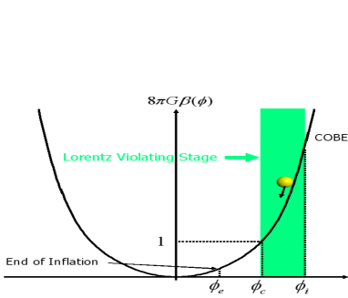
Figure 1: There is a critical point where the coupling between the Lorentz violating vector and the inflaton becomes ineffective.

When we consider the inflationary scenario, we usually require the enough e-folding number, say $N=70$. Let $\phi_{i}$ be the corresponding initial value of the scalar field. If $\phi_{c}>\phi_{i}$, the effect of Lorentz violation on the inflationary scenario would be negligible. However, if $\phi_{c}<\phi_{i}$, the standard scenario should be modified (see Fig.1). It depends on the models. To make the discussion more specific, we choose the model

$$\beta=\xi\phi^{2}\ ,\quad V=\frac{1}{2}m^{2}\phi^{2}\ ,$$ (14)

where $\xi$ and $m$ are parameters. For this model, we have

$$\phi_{c}=\frac{M_{pl}}{\sqrt{8\pi\xi}}\ .$$ (15)

As $\phi_{i}\sim 3M_{pl}$ approximately in the standard case, the condition $\phi_{i}>\phi_{c}$ implies the criterion $\xi>1/(72\pi)\sim 1/226$ for the Lorentz violation to be relevant to the inflation. For other models, the similar criterion can be easily obtained.

Now, we suppose the Lorentz violation is relevant and analyze the two regimes separately.

III.1 Lorentz violating stage

For a sufficiently larger value of $\phi$, both the coupling function $\beta$ and the potential function $V$ are important in the model (14). During this period, the effect of Lorentz violation on the inflaton dynamics must be large. In the Lorentz violating regime, $8\pi G\beta\gg 1$, we have

$$H^{2}=\frac{1}{3\beta}\left[\frac{1}{2}H^{2}\phi^{\prime 2}+V\right]$$ (16)

$$\frac{H^{\prime}}{H}+\frac{1}{2\beta}\phi^{\prime 2}+\frac{\beta^{\prime}}{\beta}=0$$ (17)

$$\phi^{\prime\prime}+\frac{H^{\prime}}{H}\phi^{\prime}+3\phi^{\prime}+\frac{V_{,\phi}}{H^{2}}+3\beta_{,\phi}=0\ .$$ (18)

To have the inflation, we impose the condition

$$H^{2}\phi^{\prime 2}\ll V$$ (19)

as the slow roll condition. Consequently, Eq.(16) is reduced to

$$H^{2}=\frac{1}{3\beta}V\ .$$ (20)

Using Eq.(20), the slow roll condition (19) can be written as

$$\phi^{\prime 2}\ll\beta\ .$$ (21)

Now, we also impose the condition $H^{\prime}/H\ll 1$ as the quasi-de Sitter condition. Then, Eq.(17) gives us the condition

$$\beta^{\prime}\ll\beta\ .$$ (22)

We also require the standard condition

$$\phi^{\prime\prime}\ll\phi^{\prime}\ .$$ (23)

Thus, we have the slow roll equations (20) and

$$\phi^{\prime}+\frac{V_{,\phi}}{3H^{2}}+\beta_{,\phi}=0\ .$$ (24)

For our example (14), we can easily solve Eqs.(20) and (24) as

$$\phi(\alpha)=\phi_{i}e^{-4\xi\alpha}\ .$$ (25)

For this solution to satisfy slow roll conditions (21)$\sim$(23), we need $\xi<1/16$. Thus, we have the range $1/226<\xi<1/16$ of the parameter for which the Lorentz violating inflation is relevant. Note that, in our model (14), the Hubble parameter (20) becomes constant

$$H^{2}=\frac{m^{2}}{6\xi}\ ,$$ (26)

even though the inflaton is rolling down the potential. This is a consequence of Lorentz violation.

III.2 Standard slow roll stage

After the inflaton crosses the critical value $\phi_{c}$, the dynamics is governed entirely by the potential $V$. In the standard slow roll regime $8\pi G\beta\ll 1$, we have

$$H^{2}=\frac{8\pi G}{3}\left[\frac{1}{2}H^{2}\phi^{\prime 2}+V\right]$$ (27)

$$\frac{H^{\prime}}{H}+4\pi G\phi^{\prime 2}=0$$ (28)

$$\phi^{\prime\prime}+\frac{H^{\prime}}{H}\phi^{\prime}+3\phi^{\prime}+\frac{V_{,\phi}}{H^{2}}=0$$ (29)

The following arguments are standard. The usual slow roll conditions give the slow roll equations

$$H^{2}=\frac{8\pi G}{3}V$$ (30)

$$\phi^{\prime}+\frac{V_{,\phi}}{3H^{2}}=0\ .$$ (31)

In the simplest case $V=\frac{1}{2}m^{2}\phi^{2}$, the evolution of the inflaton can be solved as

$$\phi^{2}(\alpha)=\phi_{c}^{2}-\frac{\alpha}{2\pi G}\ .$$ (32)

The scale factor $a(t)=e^{\alpha}$ can be also obtained as

$$a(t)=\exp\left[2\pi G(\phi_{c}^{2}-\phi^{2}(t))\right]\ .$$ (33)

The standard inflation stage ends and the reheating commences when the slow roll conditions violate.

III.3 e-folding number

Now it is easy to calculate e-folding number. Let $\phi_{i}$ be the value of the scalar field corresponding to the e-folding number $N=70$. The total e-folding number reads

$$N=\frac{1}{4\xi}\log\frac{\phi_{i}}{\phi_{c}}+2\pi G\left(\phi_{c}^{2}-\phi_{e}^{2}\right)\ ,$$ (34)

where $\phi_{e}\sim 0.3M_{pl}$ is the value of scalar field at the end of inflation. Note that the first term arises from the Lorentz violating stage. As an example, let us take the value $\xi=10^{-2}$. Then, $\phi_{c}\sim 2M_{pl}$. The contribution from the inflation end is negligible. Therefore, we get $\phi_{i}\sim 12M_{pl}$.

In this simple example, the coupling to the Lorentz violating sector disappears after the reheating. Hence, the subsequent homogeneous dynamics of the universe is the same as that of Lorentz invariant theory of gravity. However, it is possible to add some constants to $\beta_{i}$, which are consistent with the current experiments. In that case, the effect of the Lorentz violation is still relevant to the subsequent history.

So far, we have considered a special model where the coupling $\beta$ has the same power as the potential $V$. It is straightforward to extend our consideration to more general cases.

IV Lorentz Violating Inflation without Potential

In this section, we will investigate the purely Lorentz violating inflationary model.

IV.1 Exact Solutions

It is interesting to observe that we have the inflation even in the case $V=0$. In this case, Eqs.(10)$\sim$(12) reads

$$1=\frac{\phi^{\prime 2}}{6\bar{\beta}}$$ (35)

$$\frac{H^{\prime}}{H}+\frac{1}{2\bar{\beta}}\phi^{\prime 2}+\frac{\bar{\beta}^{\prime}}{\bar{\beta}}=0$$ (36)

$$\phi^{\prime\prime}+\frac{H^{\prime}}{H}\phi^{\prime}+3\phi^{\prime}+3\bar{\beta}_{,\phi}=0\ ,$$ (37)

where we have defined the variable $\bar{\beta}=\beta+1/(8\pi G)$. Substituting Eq.(35) into Eq.(36), we have

$$(\bar{\beta}H)^{\prime}+3\bar{\beta}H=0$$ (38)

It yields $\bar{\beta}H\propto e^{-3\alpha}$.

The condition for the accerelating universe $\ddot{a}>0$ is now

$$\frac{H^{\prime}}{H}>-1\ .$$ (39)

Using Eqs.(35) and (36), we can reduce the condition (39) to

$$\left(\log\bar{\beta}\right)^{\prime}<-2\ .$$ (40)

As the scalar is rolling down, Eq.(35) can be solved as $\phi^{\prime}=d\phi/d\alpha=-\sqrt{6\bar{\beta}}$. Thus, finally, we obtain the condition for $\bar{\beta}$ as

$$\sqrt{\frac{6}{\bar{\beta}}}\frac{d\bar{\beta}}{d\phi}>2\ .$$ (41)

Let us consider an exactly solvable model, $\bar{\beta}=\xi\phi^{2}$. In this simplest case, the condition (41) yields $\xi>1/6$. we can solve Eq.(35) as

$$\phi\propto e^{-\sqrt{6\xi}\alpha}\ .$$ (42)

Therefore, we have

$$H\propto e^{-\alpha/p}\ ,\quad p=\frac{1}{3-2\sqrt{6\xi}}\ .$$ (43)

There are three cases to be considered, i.e., i) $1/6<\xi<3/8$  , ii) $\xi=3/8$  , iii) $3/8<\xi$ .

i)  $1/6<\xi<3/8$

In this case, $p>0$. Hence, it is easy to solve Eq.(43)

$$\dot{\alpha}\sim e^{-\alpha/p}$$ (44)

as

$$a(t)\sim t^{p}\ ,\quad p>1\ .$$ (45)

This is a power law inflation.

ii)  $\xi=3/8$

In this case, $1/p=0$. This is nothing but the de Sitter solution

$$a(t)\sim e^{Ht}\ .$$ (46)

The Hubble constant should be determined by the initial condition. Although the spacetime itself is de Sitter, the scalar field shows the non-trivial time evolution (42). Therefore, it is interesting to calculate the curvature perturbations in this model.

iii)  $3/8<\xi$

In this case, $p\equiv-|p|<0$. Hence, the solution becomes

$$a(t)\sim(-t)^{-|p|}\ ,\quad t<0\ .$$ (47)

Thus, this solution represents the super-inflationary universe. This kind of universe encounters the singularity in the future (at $t=0$). It is possible to resolve this singularity by adding the term appeared in the string 1-loop corrections Antoniadis:1993jc ; Kawai:1998bn . It is also important to study if the behavior of perturbations also similar or not Kawai:1998ab ; Kawai:1999pw .

IV.2 Inflationary scenario

In the absence of the inflaton potential, we have obtained exact solutions , i.e., the power law inflation, the de Sitter inflation, and the super-inflation . If we slightly modify $\bar{\beta}$, the inflation will end when the condition (41) violates. Note that, when the scalar varies from $\phi_{i}$ to $\phi_{e}$, the e-folding number of the universe can be calculated as

$$N=\frac{1}{\sqrt{6\xi}}\log\frac{\phi_{i}}{\phi_{e}}\ .$$ (48)

We expect that the reheating would occur during the oscillation phase. It should be stressed that the above inflations are completely associated with the Lorentz violation.

V Evolution of Tensor Perturbations

Needless to say, it needs to study the evolution of cosmological perturbations. Due to the Lorentz violation, the velocity of the gravitational waves are different from the velocity of the light. This and the non-trivial coupling functions $\beta_{i}$ would cause interesting consequence on the spectrum of tensor, vector and scalar perturbations. In particular, the vector perturbations are intriguing since there are no vector perturbations in the Lorentz invariant inflationary scenario. However, as the calculation is very complicated, we leave the complete analysis for future publication. Instead, here, we discuss the simplest case, namely tensor perturbations. Even in this case, we can make some interesting predictions.

The tensor part of perturbations can be described by

$$ds^{2}=-dt^{2}+a^{2}(t)\left(\delta_{ij}+h_{ij}(t,x^{i})\right)dx^{i}dx^{j}\ ,$$ (49)

where the perturbation satisfy $h^{i}{}_{i}=h_{ij}{}^{,j}=0$. The quadratic part of the action is given by

$$S=\int d^{4}x\frac{a^{3}}{16\pi G}\left[\frac{1}{4}\gamma\dot{h}_{ij}\dot{h}^{\prime ij}-\frac{1}{4a^{2}}h_{ij,k}h^{ij,k}\right]$$ (50)

where we have defined

$$\gamma=1-16\pi G(\beta_{1}+\beta_{3})\ .$$ (51)

Apparently, the velocity of the gravitational waves is not 1. To have the real velocity, we have to impose $\gamma>0$. Hence, we assume $\beta_{1}$ and $\beta_{3}$ are constant.

In the case of chaotic inflation model, the Hubble parameter is constant (26) during Lorentz violating stage. The spectrum is completely flat although the inflaton is rolling down the potential. This is a clear prediction of the Lorentz violating chaotic inflation.

This same result applies to the exact de Sitter inflation model without the potential. In the case of the power law and the super inflation models, the spectrum of the primordial gravitational waves are tilted.

VI Conclusion

We have examined the impact of Lorentz violation on the inflationary scenario. As a specific model, we have considered the spontaneous violation of the Lorentz symmetry due to the vector field. More specifically, we have investigated scalar-vector-tensor theory of gravity where the vector is constrained to be unit and time-like.

First, we have examined the chaotic inflationary scenario and found that the Lorentz violation modifies the dynamics of the inflaton for a certain parameter region in our model. We have shown that the inflationary stage breaks into two parts; the Lorentz violating stage and the standard slow roll stage. We found that the universe is expanding as an exact de Sitter spacetime in the Lorentz violating stage although the inflaton field is rolling down the potential. Moreover, we have calculated the e-folding number by taking into account the above modification and shown that we can get enough e-folding number.

In this paper, we have considered the simplest case $\beta\sim V\sim\phi^{2}$. In other cases, for instance, $\beta\sim\phi^{4}$ and $V\sim\phi^{2}$, the Hubble parameter $H$ increases during the Lorentz violating stage. In the standard slow roll stage, the Hubble parameter $H$ decreases. Therfore, we can easily generate the spectrum with the initial (steep) blue spectrum and the later (slightly) red spectrum. This may explain the deficiency of the CMB power spectrum at large scales observed by WMAP Bennett:2003bz .

We have also shown that the inflation can be realized without the inflaton potential. Depending on the value of the parameter $\xi$, we have obtained exact solutions, i.e. the power law inflation, de Sitter inflation, and the super inflation. Interestingly, even in the exact de Sitter case, the dynamics of the scalar field turns out to be non-trivial. In all cases, the inflation ends when the coupling function $\bar{\beta}$ is slightly modified from exactly solvable case. These exactly solvable models are important to understand the evolution of cosmological perturbations in the Lorentz violating theory of gravity.

To discuss the observability of the effect of Lorentz violation, we calculated the tensor perturbations and found the extremely flat spectrum although the inflaton rolls down the potential in the case of the chaotic inflation model. This same result applies to the exact de Sitter inflation model without the potential. This is a clear prediction of Lorentz violating inflation model.

It would be interesting to study the evolution of fluctuation completely. If the vector modes of perturbations can survive till the last scattering surface, they leave the remnant of the Lorentz violation on the CMB polarization spectrum. It is also intriguing to seek for a relation to the large scale anomaly discovered in CMB by WMAP Eriksen:2003db ; deOliveira-Costa:2003pu ; Land:2005ad ; Copi:2005ff . The calculation of the curvature perturbation is much more complicated. However, it must reveal more interesting phenomena due to Lorentz violating inflation. The tensor-scalar ratio of the power spectrum would be also interesting. These are now under investigation kanno .

Appendix A Alignment of preferred frames

Here, we would like to show the alignment of two frames, the CMB rest frame and the frame determined by $u^{\mu}$, will occur during the cosmological evolution. For simplicity, we ignore the scalar field, instead we add the cosmological constant term to the action. The action is

$$S = \int d^{4}x\sqrt{-g}\left[\frac{1}{16\pi G}\left(R-2\Lambda\right)-\beta_{1}\nabla^{\mu}u^{\nu}\nabla_{\mu}u_{\nu}\right.$$ (52)

$$\left.\qquad\qquad\qquad-\beta_{2}\nabla^{\mu}u^{\nu}\nabla_{\nu}u_{\mu}-\beta_{3}\left(\nabla_{\mu}u^{\mu}\right)^{2}\right.$$

$$\left.\qquad\qquad\qquad-\beta_{4}u^{\mu}u^{\nu}\nabla_{\mu}u^{\alpha}\nabla_{\nu}u_{\alpha}\right.$$

$$\left.\qquad\qquad\qquad+\lambda\left(u^{\mu}u_{\mu}+1\right)\right]\ .$$

We consider the Bianchi Type I metric as an ansatz:

$$ds^{2} = -{\cal N}^{2}(t)dt^{2}+e^{2\alpha(t)}\left[e^{-4\sigma_{+}(t)}dx^{2}\right.$$ (53)

$$\left.+e^{2\sigma_{+}(t)}\left\{e^{2\sqrt{3}\sigma_{-}(t)}dy^{2}+e^{-2\sqrt{3}\sigma_{-}(t)}dz^{2}\right\}\right]\qquad$$

and now the vector field can be tilted as

$$u^{\mu}=\left(\frac{1}{{\cal N}(t)}\cosh\theta(t),e^{-\alpha(t)+2\sigma_{+}(t)}\sinh\theta(t),0,0\right)\ .\quad$$ (54)

Thus, in general, the cosmic frame is different from the preferred frame determined by $u^{\mu}$. Substituting the metric and the vector field into the action (A1), we obtain

$$S = \int dt\frac{1}{\cal N}e^{3\alpha}\left[-A\dot{\alpha}^{2}-\lambda{\cal N}^{2}+B\left(\dot{\sigma}_{+}^{2}+\dot{\sigma}_{-}^{2}\right)\right.$$ (55)

$$\left.\qquad\qquad\qquad+D\dot{\theta}^{2}-E\theta\dot{\theta}\dot{\alpha}-F\theta^{2}\dot{\alpha}^{2}\right]\ ,$$

where

$$A = \frac{3}{8\pi G}\left\{1+8\pi G\left(\beta_{1}+3\beta_{2}+\beta_{3}\right)\right\}\ ,$$ (56)

$$B = \frac{3}{8\pi G}\left\{1-16\pi G\left(\beta_{1}+\beta_{3}\right)\right\}\ ,$$ (57)

$$D = \beta_{1}-\beta_{4}\ ,$$ (58)

$$E = 2\left(3\beta_{2}+\beta_{3}+\beta_{4}\right)\ ,$$ (59)

$$F = 2\beta_{1}+9\beta_{2}+3\beta_{3}+\beta_{4}\ ,$$ (60)

$$\lambda = \frac{\Lambda}{8\pi G}\ .$$ (61)

By taking the variation of (A4), we obtain

$$A\dot{\alpha}^{2}-\lambda=0\ ,$$ (62)

$$\frac{d}{dt}\left(e^{3\alpha}\dot{\sigma}_{\pm}\right)=0\ ,$$ (63)

$$A\frac{d}{dt}\left(e^{3\alpha}\dot{\alpha}\right)-3\lambda e^{3\alpha}=0\ ,$$ (64)

$$E\theta\frac{d}{dt}\left(e^{3\alpha}\dot{\alpha}\right)-2D\frac{d}{dt}\left(e^{3\alpha}\dot{\theta}\right)-2Fe^{3\alpha}\theta\dot{\alpha}^{2}=0\ ,\quad\qquad$$ (65)

where we kept up to the first order with respect to $\sigma_{\pm}$ and $\theta$. From Eq.(A12), it turns out that the anisotropy decays as the universe expands. Now, we can deduce the master equation for the tilt $\theta$ as

$$\ddot{\theta}+3\dot{\alpha}\dot{\theta}+\left(\frac{F}{D}\dot{\alpha}^{2}-\frac{3E}{2AD}\lambda\right)\theta=0\ .$$ (66)

Using Eq.(A11) and the definitions (A8) and (A9), we have

$$\ddot{\theta}+3\dot{\alpha}\dot{\theta}+\frac{2\lambda}{A}\theta=0\ .$$ (67)

For the effective gravitational coupling to be positive, we need $A>0$. Thus, (A16) tells us that the tilt $\theta$ will vanish during the cosmic expansion.

Namely, the CMB rest frame and the preferred frame determined by $u^{\mu}$ are the same practically. What we did in this paper is to reveal what this degeneracy means in inflationary cosmology.

References

- (1) Greisen, Phys.Lett.16, 148.
- (2) G. T. Zatsepin and V. A. Kuzmin, JETP Lett. 4, 78 (1966) [Pisma Zh. Eksp. Teor. Fiz. 4, 114 (1966)].
- (3) M. Takeda et al., Phys. Rev. Lett. 81, 1163 (1998) [arXiv:astro-ph/9807193].
- (4) H. Sato, arXiv:astro-ph/0005218.
- (5) S. R. Coleman and S. L. Glashow, Phys. Rev. D 59, 116008 (1999) [arXiv:hep-ph/9812418].
- (6) G. Amelino-Camelia, J. R. Ellis, N. E. Mavromatos, D. V. Nanopoulos and S. Sarkar, Nature 393, 763 (1998) [arXiv:astro-ph/9712103].
- (7) V. A. Kostelecky and S. Samuel, Phys. Rev. D 39, 683 (1989).
- (8) J. D. Bekenstein, Phys. Rev. D 70, 083509 (2004) [Erratum-ibid. D 71, 069901 (2005)] [arXiv:astro-ph/0403694].
- (9) S. M. Carroll and J. Shu, arXiv:hep-ph/0510081.
- (10) S. M. Carroll and E. A. Lim, Phys. Rev. D 70, 123525 (2004) [arXiv:hep-th/0407149].
- (11) D. Mattingly, Living Rev. Rel. 8, 5 (2005) [arXiv:gr-qc/0502097].
- (12) N. Arkani-Hamed, H. C. Cheng, M. A. Luty and S. Mukohyama, JHEP 0405, 074 (2004) [arXiv:hep-th/0312099].
- (13) N. Arkani-Hamed, H. C. Cheng, M. Luty and J. Thaler, JHEP 0507, 029 (2005) [arXiv:hep-ph/0407034].
- (14) H. C. Cheng, M. A. Luty, S. Mukohyama and J. Thaler, arXiv:hep-th/0603010.
- (15) N. Arkani-Hamed, P. Creminelli, S. Mukohyama and M. Zaldarriaga, JCAP 0404, 001 (2004) [arXiv:hep-th/0312100].
- (16) C. Csaki, J. Erlich and C. Grojean, Nucl. Phys. B 604, 312 (2001) [arXiv:hep-th/0012143].
- (17) J. M. Cline and L. Valcarcel, JHEP 0403, 032 (2004) [arXiv:hep-ph/0312245].
- (18) M. V. Libanov and V. A. Rubakov, Phys. Rev. D 72, 123503 (2005) [arXiv:hep-ph/0509148].
- (19) B. M. Gripaios, JHEP 0410, 069 (2004) [arXiv:hep-th/0408127].
- (20) T. Jacobson and D. Mattingly, Phys. Rev. D 64, 024028 (2001) [arXiv:gr-qc/0007031].
- (21) C. Eling and T. Jacobson, Phys. Rev. D 69, 064005 (2004) [arXiv:gr-qc/0310044].
- (22) M. L. Graesser, A. Jenkins and M. B. Wise, Phys. Lett. B 613, 5 (2005) [arXiv:hep-th/0501223].
- (23) B. Z. Foster and T. Jacobson, Phys. Rev. D 73, 064015 (2006) [arXiv:gr-qc/0509083].
- (24) B. Z. Foster, arXiv:gr-qc/0602004.
- (25) E. A. Lim, Phys. Rev. D 71, 063504 (2005) [arXiv:astro-ph/0407437].
- (26) J. W. Elliott, G. D. Moore and H. Stoica, JHEP 0508, 066 (2005) [arXiv:hep-ph/0505211].
- (27) T. Futamase and K. i. Maeda, Phys. Rev. D 39, 399 (1989).
- (28) R. Fakir and W. G. Unruh, Phys. Rev. D 41, 1783 (1990).
- (29) I. Antoniadis, J. Rizos and K. Tamvakis, Nucl. Phys. B 415, 497 (1994) [arXiv:hep-th/9305025].
- (30) S. Kawai and J. Soda, Phys. Rev. D 59, 063506 (1999) [arXiv:gr-qc/9807060].
- (31) S. Kawai, M. a. Sakagami and J. Soda, Phys. Lett. B 437, 284 (1998) [arXiv:gr-qc/9802033].
- (32) S. Kawai and J. Soda, Phys. Lett. B 460, 41 (1999) [arXiv:gr-qc/9903017].
- (33) C. L. Bennett et al., Astrophys. J. Suppl. 148, 1 (2003) [arXiv:astro-ph/0302207].
- (34) H. K. Eriksen, F. K. Hansen, A. J. Banday, K. M. Gorski and P. B. Lilje, Astrophys. J. 605, 14 (2004) [Erratum-ibid. 609, 1198 (2004)] [arXiv:astro-ph/0307507].
- (35) A. de Oliveira-Costa, M. Tegmark, M. Zaldarriaga and A. Hamilton, Phys. Rev. D 69, 063516 (2004) [arXiv:astro-ph/0307282].
- (36) K. Land and J. Magueijo, Phys. Rev. Lett. 95, 071301 (2005) [arXiv:astro-ph/0502237].
- (37) C. J. Copi, D. Huterer, D. J. Schwarz and G. D. Starkman, Mon. Not. Roy. Astron. Soc. 367, 79 (2006) [arXiv:astro-ph/0508047].
- (38) S. Kanno and J.Soda, in preparation.