SWAT 06/463
DAMTP-2006-28
hep-th/0604156
Nonequilibrium dynamics in the $O(N)$ model to next-to-next-to-leading order in the $1/N$ expansion

Gert Aartsa and Anders Tranbergb,c

aDepartment of Physics, University of Wales Swansea
Singleton Park, Swansea, SA2 8PP, United Kingdom

bDepartment of Physics & Astronomy, University of Sussex
Falmer, Brighton, BN1 9QH, United Kingdom

cDAMTP, University of Cambridge
Wilberforce Road, Cambridge, CB3 0WA, United Kingdom
email: g.aarts@swan.ac.ukemail: a.tranberg@damtp.cam.ac.uk
(April 21, 2006)
Abstract

Nonequilibrium dynamics in quantum field theory has been studied extensively using truncations of the 2PI effective action. Both $1/N$ and loop expansions beyond leading order show remarkable improvement when compared to mean-field approximations. However, in truncations used so far, only the leading-order parts of the self energy responsible for memory loss, damping and equilibration are included, which makes it difficult to discuss convergence systematically. For that reason we derive the real and causal evolution equations for an $O(N)$ model to next-to-next-to-leading order in the 2PI-$1/N$ expansion. Due to the appearance of internal vertices the resulting equations appear intractable for a full-fledged $3+1$ dimensional field theory. Instead, we solve the closely related three-loop approximation in the auxiliary-field formalism numerically in $0+1$ dimensions (quantum mechanics) and compare to previous approximations and the exact numerical solution of the SchrΓΆdinger equation.

1 Introduction

The two-particle irreducible (2PI) effective action formalism has proven very powerful for out-of-equilibrium quantum field theory over a wide range of applications [1]. Since it necessarily employs an expansion and truncation of the effective action, one should be concerned with how well these expansions converge.333Of course, perturbative or $1/N$ expansions in quantum mechanics and field theory are usually not convergent but instead asymptotic, see e.g. ref. [2] for discussions concerning the $O(N)$ model.

An extensive study has been made of effective mean-field approximations (Gaussian, leading order (LO) $1/N$ or Hartree approximations) which amounts to including a self-consistent, time-dependent effective mass in the dynamics of the one- and two-point functions [3]. However, since such an approximation does not include scattering, phenomena such as damping, memory loss and equilibration cannot be described properly. This can be traced back to the existence of (infinitely many) conserved charges in the mean-field dynamics and the presence of a nonthermal fixed point [4, 5].444Some scattering is present if one allows for inhomogeneous mean fields [6, 7, 8]. Going beyond the mean-field approximation, by either employing the weak-coupling or the $1/N$ expansion to next-to-leading order (NLO), effective memory loss, damping and equilibration are present.555See e.g. refs. [9, 10, 11, 12] for the loop expansion, refs. [13, 14, 15, 16, 17, 18, 19, 20] for the 2PI-$1/N$ expansion to NLO, and ref. [21] for 2PI dynamics with fermions. In particular it has been found that at late times the system evolves towards a quantum equilibrium state, characterized by suitably defined field occupation numbers approaching the familiar Bose-Einstein or Fermi-Dirac distribution functions. The self-consistently determined propagators have a time-dependent mass and width. It is found therefore that NLO approximations improve dramatically upon mean-field approximations and qualitatively reproduce the dynamics expected on physical grounds from the full, untruncated system.

The natural question to ask is whether a truncation at NLO also gives quantitatively correct results. This issue has been investigated in several ways, usually by comparing the NLO results to other available approximations. For example, when the coupling is small, normal perturbation theory should be applicable for e.g. estimates of damping rates. Indeed, the results in ref. [12] suggest that the perturbative result is reproduced within a factor of two for small coupling, where the difference is due to the effect of including self-consistent infinite resummations in the 2PI approach. However, this amounts to a test of perturbation theory rather than a verification of the 2PI formalism. Similarly, it is well-known [22] how to derive on-shell kinetic (Boltzmann) equations from truncations of the 2PI effective action and one can compare the self-consistent 2PI dynamics with dynamics from kinetic theory [11, 23, 24]. However, this again serves more as a test of kinetic theory than of the 2PI truncation. Another possibility, relevant for the dynamics at very late times, is to study transport coefficients from the 2PI effective action, which gives insight into what scattering processes are included [25, 26].

When the exact, untruncated evolution is accessible, one may carry out a direct comparison. This option is available in quantum mechanics, where the dynamics from the 2PI effective action can be benchmarked against the numerical solution of the SchrΓΆdinger equation [27]. Finally, perhaps the most detailed comparison has been made within classical statistical field theory, where direct numerical simulations are straightforward [5]. Moreover, the 2PI formalism can be easily applied to classical dynamics of an initial nonequilibrium ensemble [15, 16, 20].666In quantum field theory, stochastic quantization techniques have recently yielded the first real-time nonequilibrium lattice simulation results [28]. When developed further, this would offer the possibility for direct tests as well. In ref. [15] it was found in the context of the $1+1$ dimensional $O(N)$ model that the nonperturbative classical evolution, obtained numerically, is well reproduced by the 2PI-$1/N$ expansion at NLO for $N$ larger than about $10$, providing direct support for the use of the 2PI-$1/N$ approximation at NLO.

Refer to caption

Figure 1: Weak-coupling expansion of the 2PI effective action in the broken phase of a scalar $\lambda\phi^{4}$ theory [12].

Ideally, within a given approximation scheme, the validity of a truncation is estimated by extending the method to the next order in the expansion and test for effective convergence. Due to the absence of scattering in mean-field approximations, it is essential to go to NLO and compare NLO with approximations that go further. In the coupling expansion, a first attempt to do this was made in ref. [12]. Here it was noted that in the broken phase of a $\lambda\phi^{4}$ theory two diagrams contribute at $\mathcal{O}(\lambda)$: the Hartree and the background field dependent diagram, shown in fig. 1 on the left. Perturbatively neither of these diagrams leads to (on-shell) damping, but after the self-consistent 2PI resummation the second one does. This approximation can then be extended by inclusion of the basketball diagram, shown in fig. 1 on the right. From a comparison between the dynamical evolution in the two truncations, it was found that equilibration times differ, but only by a factor less than two, see ref. [12] for more details. Both truncations are at the level of complexity of the 2PI-$1/N$ expansion to NLO and are therefore numerically tractable. Technically, the common feature of these truncations, and in fact of all truncations treated so far, is the absence of internal vertices in self energies. This is important from a numerical point of view, which is complicated due to the presence of memory integrals in the evolution equations. Additional vertices require extra memory integrals to be carried out, which is numerically expensive.

In this paper we extend the analysis and include for the first time self energies with internal vertices, using the framework of the 2PI-$1/N$ expansion to next-to-next-to-leading order (N2LO) in the symmetric phase of the $O(N)$ model. This opens up the possibility to make a quantitative comparison between evolution at NLO and N2LO in the $1/N$ expansion. The N2LO effective equations of motion contain additional (nested) space-time integrals for each time step, when compared to NLO. It is beyond the scope of this paper to solve those equations in full field theory. For the sake of illustration we instead specialise to quantum mechanics which allows us to test the consistency of the equations, the conservation of energy and effective convergence of the expansion. We stress that the dynamics of quantum mechanics is of course very different from field theory. Given sufficient computer power the evolution equations can readily be implemented in field theory.

The paper is organized as follows. In the next section we briefly review the 2PI-$1/N$ expansion in the $O(N)$ model, following closely the discussion and notation of ref. [17]. In section 3 we present the dynamical equations to N2LO and give explicitly (part of) the statistical and spectral self energies, which are much more involved than at NLO due to the presence of internal vertices. Results from the numerical implementation for the $0+1$ dimensional case are shown in section 4, while the outlook is given in section 5. In three appendices we collect technicalities related to the standard loop expansion, multi-loop contour integrals and the numerical solution of the SchrΓΆdinger equation.

2 2PI-$1/N$ expansion

Throughout the paper we consider an $N$ component scalar field in the $O(N)$ symmetric phase ($\langle\phi_{a}\rangle=0$). The action is

$$S=-\int_{\mathcal{C}}d^{4}x\left[\frac{1}{2}\partial_{\mu}\phi_{a}\partial^{\mu}\phi_{a}+\frac{1}{2}m^{2}\phi_{a}\phi_{a}+\frac{\lambda}{4!N}(\phi_{a}\phi_{a})^{2}\right],$$ (2.1)

with $a=1,\ldots,N$. Doubled indices are summed over. As appropriate to an out-of-equilibrium treatment, the fields are defined along the Keldysh contour $\mathcal{C}$ in the complex-time plane, see appendix B. The 2PI effective action depends on the full two-point function $G$ of the theory and can be parametrised as [29]

$$\Gamma[G]=\frac{i}{2}\mbox{Tr}\ln G^{-1}+\frac{i}{2}\mbox{Tr}\,G_{0}^{-1}\left(G-G_{0}\right)+\Gamma_{2}[G],$$ (2.2)

where $G_{0}^{-1}$ denotes the free inverse propagator. Variation of the effective action with respect to $G$ results in the Schwinger-Dyson equation for the two-point function, $G^{-1}=G_{0}^{-1}-\Sigma$, which after multiplication with $G$ reads

$$-\left[\square_{x}+m^{2}\right]G_{ab}(x,y)=i\int_{z}\Sigma_{ac}(x,z)G_{cb}(z,y)+i\delta_{ab}\delta_{{\cal C}}(x-y).$$ (2.3)

Here we used the short-hand notation

$$\int_{z}=\int_{\cal C}d^{4}z.$$ (2.4)

The self energy is given by

$$\Sigma_{ab}=2i\frac{\delta\Gamma_{2}[G]}{\delta G_{ab}}.$$ (2.5)

The full four-point function is represented by the nonlocal term on the RHS of eq. (2.3). For future reference we note here that

$$\frac{\lambda}{6N}\langle\phi_{a}^{2}(x)\phi_{c}^{2}(x)\rangle=i\int_{\cal C}d^{4}z\,\Sigma_{ac}(x,z)G_{ca}(z,x),$$ (2.6)

which can be verified using e.g. the Heisenberg equations of motion.

To implement the $1/N$ expansion efficiently, it is convenient to use the auxiliary-field formalism [30, 31, 14, 17]. The action then reads

$$S[\phi,\chi]=-\int_{x}\left[\frac{1}{2}\partial_{\mu}\phi_{a}\partial^{\mu}\phi_{a}+\frac{1}{2}m^{2}\phi_{a}\phi_{a}-\frac{3N}{2\lambda}\chi^{2}+\frac{1}{2}\chi\phi_{a}\phi_{a}\right].$$ (2.7)

Integrating out $\chi$ yields the original action (2.1). The 2PI effective action is now written in terms of the one-point function $\bar{\chi}=\langle\chi(x)\rangle$ and the two-point functions

$$G_{ab}(x,y)=\langle T_{\cal C}\phi_{a}(x)\phi_{b}(y)\rangle,\;\;\;\;\;\;\;\;D(x,y)=\langle T_{\cal C}\chi(x)\chi(y)\rangle-\langle\chi(x)\rangle\langle\chi(y)\rangle,$$ (2.8)

and reads

$\displaystyle\Gamma[G,D,\bar{\chi}]=$ $\displaystyle S[0,\bar{\chi}]+\frac{i}{2}\mbox{Tr}\ln G^{-1}+\frac{i}{2}\mbox{Tr}\,G_{0}^{-1}\left(G-G_{0}\right)$ (2.9)
$\displaystyle+\frac{i}{2}\mbox{Tr}\ln D^{-1}+\frac{i}{2}\mbox{Tr}\,D_{0}^{-1}\left(D-D_{0}\right)+\Gamma_{2}[G,D].$

Since we take $\langle\phi_{a}\rangle=0$, there is no mixing between the $\phi$ and $\chi$ propagators [14, 17]. The free inverse propagators read

$$G_{0,ab}^{-1}(x,y)=i\left[\square_{x}+m^{2}+\bar{\chi}(x)\right]\delta_{ab}\delta_{\cal C}(x-y),\;\;\;\;\;\;\;\;D_{0}^{-1}(x,y)=\frac{3N}{i\lambda}\delta_{\cal C}(x-y).$$ (2.10)

The evolution equations for the propagators $G$ and $D$ and the one-point function $\bar{\chi}$ are obtained by extremizing (2.9) and read

$\displaystyle-\left[\square_{x}+m^{2}+\bar{\chi}(x)\right]G_{ab}(x,y)=$ $\displaystyle i\int_{z}\Sigma_{ac}(x,z)G_{cb}(z,y)+i\delta_{ab}\delta_{\cal C}(x-y),$
$\displaystyle\frac{3N}{\lambda}D(x,y)=$ $\displaystyle i\int_{z}\Pi(x,z)D(z,y)+i\delta_{\cal C}(x-y),$ (2.11)

and

$$\bar{\chi}(x)=\frac{\lambda}{6N}G_{cc}(x,x).$$ (2.12)

Refer to caption

Figure 2: NLO (2 loops) and N2LO (3 and 4 loops) contributions in the 2PI-$1/N$ expansion. The scalar propagator $G$ is denoted with the full line and the auxiliary-field propagator $D$ with the dashed line.

The self energies are defined by

Ξ£a​b=2​i​δ​Γ2​[G,D]δ​Ga​b,Ξ =2​i​δ​Γ2​[G,D]δ​D.formulae-sequencesubscriptΞ£π‘Žπ‘2𝑖𝛿subscriptΞ“2𝐺𝐷𝛿subscriptπΊπ‘Žπ‘Ξ 2𝑖𝛿subscriptΞ“2𝐺𝐷𝛿𝐷\Sigma_{ab}=2i\frac{\delta\Gamma_{2}[G,D]}{\delta G_{ab}},\;\;\;\;\;\;\;\;\;\;\;\;\;\;\;\;\Pi=2i\frac{\delta\Gamma_{2}[G,D]}{\delta D}. (2.13)

It is convenient to separate the local part of $D$ [17] and write

$$D(x,y)=\frac{\lambda}{3N}\left[i\delta_{{\cal C}}(x-y)+\hat{D}(x,y)\right],$$ (2.14)

such that $\hat{D}$ is determined from

$$\hat{D}(x,y)=-\frac{\lambda}{3N}\Pi(x,y)+\frac{i\lambda}{3N}\int_{z}\Pi(x,z)\hat{D}(z,y).$$ (2.15)

We now continue with the 2PI-$1/N$ expansion, in which there is one diagram at NLO and two diagrams at N2LO, see fig. 2. For a detailed powercounting discussion we refer to ref. [17]. It suffices here to say that a closed scalar propagator $G\sim N$ and the auxiliary-field propagator $D\sim 1/N$. It is then easy to see that diagram $(2)\sim 1$ and diagrams $(3)$ and $(4)\sim 1/N$. The expressions are

$\displaystyle\Gamma_{2}^{\rm NLO}[G,D]=$ $\displaystyle\frac{i}{4}\int_{xy}G_{ab}^{2}(x,y)D(x,y),$ (2.16)
$\displaystyle\Gamma_{2}^{\rm NNLO(3)}[G,D]=$ $\displaystyle-\frac{i}{8}\int_{xyzw}G_{ab}(x,y)G_{bc}(y,z)G_{cd}(z,w)G_{da}(w,x)D(x,z)D(y,w),$
$\displaystyle\Gamma_{2}^{\rm NNLO(4)}[G,D]=$ $\displaystyle\frac{i}{12}\int_{xyzx^{\prime}y^{\prime}z^{\prime}}G_{ab}(x,y)G_{bc}(y,z)G_{ca}(z,x)$
$\displaystyle\times G_{a^{\prime}b^{\prime}}(x^{\prime},y^{\prime})G_{b^{\prime}c^{\prime}}(y^{\prime},z^{\prime})G_{c^{\prime}a^{\prime}}(z^{\prime},x^{\prime})D(x,x^{\prime})D(y,y^{\prime})D(z,z^{\prime}).$

The corresponding self energies are shown in figs. 4 and 4.

Refer to caption

Figure 3: Self energy $\Sigma$ at NLO (1 loop) and N2LO (2 and 3 loops).

Refer to caption

Figure 4: Auxiliary-field self energy Ξ Ξ \Pi at NLO (1 loop) and N2LO (2 and 3 loops).

We continue with the $O(N)$ symmetric case, such that $G_{ab}(x,y)=G(x,y)\delta_{ab}$ and $\Sigma_{ab}(x,y)=\Sigma(x,y)\delta_{ab}$. For notational simplicity we label the self energies according to the number of loops, e.g. $\Sigma^{({\ell})}$, where ${\ell}=1,2,3$. We stress that the 2PI-$1/N$ expansion does not coincide with loop expansion in the auxiliary-field formalism. For instance, there are two more four-loop diagrams, see fig. 5, which only contribute at N3LO. The connection with the standard loop expansion is discussed further in appendix A.

At NLO the self energies read

$\displaystyle\Sigma^{(1)}(x,y)=$ $\displaystyle-G(x,y)D(x,y),$ (2.17)
Ξ (1)​(x,y)=superscriptΞ 1π‘₯𝑦absent\displaystyle\Pi^{(1)}(x,y)= $\displaystyle-\frac{N}{2}G^{2}(x,y),$ (2.18)

and at N2LO

$\displaystyle\Sigma^{(2)}(x,y)=$ $\displaystyle\int_{zw}G(x,w)G(w,z)G(z,y)D(x,z)D(w,y),$ (2.19)
$\displaystyle\Sigma^{(3)}(x,y)=$ $\displaystyle-N\int_{zx^{\prime}y^{\prime}z^{\prime}}\!\!\!\!\!\!\!\!G(x,z)G(z,y)G(x^{\prime},y^{\prime})G(y^{\prime},z^{\prime})G(z^{\prime},x^{\prime})D(x,x^{\prime})D(y,y^{\prime})D(z,z^{\prime}),$
Ξ (2)​(x,y)=superscriptΞ 2π‘₯𝑦absent\displaystyle\Pi^{(2)}(x,y)= $\displaystyle\frac{N}{2}\int_{zw}G(x,w)G(w,y)G(x,z)G(z,y)D(z,w),$ (2.20)
Ξ (3)​(x,y)=superscriptΞ 3π‘₯𝑦absent\displaystyle\Pi^{(3)}(x,y)= $\displaystyle-\frac{N^{2}}{2}\int_{zz^{\prime}ww^{\prime}}\!\!\!\!\!\!\!\!\!\!\!G(x,z)G(z,w)G(w,x)G(y,z^{\prime})G(z^{\prime},w^{\prime})G(w^{\prime},y)D(w,w^{\prime})D(z,z^{\prime}).$

Refer to caption

Figure 5: Loop expansion in the auxiliary-field formalism: additional four-loop diagrams, of order $1/N^{2}$ (N3LO).

3 Causal equations

To bring the evolution equations in a form that can be solved numerically, the contour propagators and self energies are written in terms of statistical ($F$) and spectral ($\rho$) components [10],

$$G(x,y)=F(x,y)-\frac{i}{2}\mbox{sgn}_{\cal C}(x,y)\rho(x,y),$$ (3.1)

and similar for $\hat{D}$, $\Sigma$ and Ξ Ξ \Pi. Here $\mbox{sgn}_{\cal C}(x,y)=\Theta_{{\cal C}}(x^{0}-y^{0})-\Theta_{{\cal C}}(y^{0}-x^{0})$ is the sign-function along the contour, see appendix B. The explicitly causal equations then read [17]

$\displaystyle\left[\square_{x}+M^{2}(x)\right]\rho(x,y)=$ $\displaystyle-\int_{y^{0}}^{x^{0}}dz\,\Sigma_{\rho}(x,z)\rho(z,y),$ (3.2)
$\displaystyle\left[\square_{x}+M^{2}(x)\right]F(x,y)=$ $\displaystyle-\int_{0}^{x^{0}}dz\,\Sigma_{\rho}(x,z)F(z,y)+\int_{0}^{y^{0}}dz\,\Sigma_{F}(x,z)\rho(z,y),$

where

$$M^{2}(x)=m^{2}+\lambda\frac{N+2}{6N}F(x,x),$$ (3.3)

and

$\displaystyle\frac{3N}{\lambda}\hat{D}_{\rho}(x,y)=$ βˆ’Ξ Οβ€‹(x,y)+∫y0x0𝑑z​Πρ​(x,z)​D^ρ​(z,y),subscriptΠ𝜌π‘₯𝑦superscriptsubscriptsuperscript𝑦0superscriptπ‘₯0differential-d𝑧subscriptΠ𝜌π‘₯𝑧subscript^π·πœŒπ‘§π‘¦\displaystyle-\Pi_{\rho}(x,y)+\int_{y^{0}}^{x^{0}}dz\,\Pi_{\rho}(x,z)\hat{D}_{\rho}(z,y), (3.4)
$\displaystyle\frac{3N}{\lambda}\hat{D}_{F}(x,y)=$ βˆ’Ξ F​(x,y)+∫0x0𝑑z​Πρ​(x,z)​D^F​(z,y)βˆ’βˆ«0y0𝑑z​ΠF​(x,z)​D^ρ​(z,y).subscriptΠ𝐹π‘₯𝑦superscriptsubscript0superscriptπ‘₯0differential-d𝑧subscriptΠ𝜌π‘₯𝑧subscript^𝐷𝐹𝑧𝑦superscriptsubscript0superscript𝑦0differential-d𝑧subscriptΠ𝐹π‘₯𝑧subscript^π·πœŒπ‘§π‘¦\displaystyle-\Pi_{F}(x,y)+\int_{0}^{x^{0}}dz\,\Pi_{\rho}(x,z)\hat{D}_{F}(z,y)-\int_{0}^{y^{0}}dz\,\Pi_{F}(x,z)\hat{D}_{\rho}(z,y).

We use here the notation

$$\int_{y^{0}}^{x^{0}}dz=\int_{y^{0}}^{x^{0}}dz^{0}\int d^{3}z.$$ (3.5)

Equations of motion derived from truncations of the 2PI effective action conserve the following energy functional (cf. eq. (2.6)),

$\displaystyle E/N=$ $\displaystyle\int d^{3}x\,\frac{1}{2}\left[\partial_{x^{0}}\partial_{y^{0}}+\partial_{x^{i}}\partial_{y^{i}}+m^{2}+\frac{\lambda}{12}\frac{N+2}{N}F(x,x)\right]F(x,y)\Big{|}_{x=y}$ (3.6)
$\displaystyle+\frac{1}{4}\int d^{3}x\int_{0}^{x^{0}}dz^{0}\int d^{3}z\,\left[\Sigma_{\rho}(x,z)F(z,x)-\Sigma_{F}(x,z)\rho(z,x)\right].$

The statistical and spectral self energies at NLO can be found in ref. [17] and read

$\displaystyle\Sigma_{F}^{(1)}(x,y)=$ $\displaystyle-\frac{\lambda}{3N}\left[F(x,y)\hat{D}_{F}(x,y)-\frac{1}{4}\rho(x,y)\hat{D}_{\rho}(x,y)\right],$
$\displaystyle\Sigma_{\rho}^{(1)}(x,y)=$ $\displaystyle-\frac{\lambda}{3N}\left[\rho(x,y)\hat{D}_{F}(x,y)+F(x,y)\hat{D}_{\rho}(x,y)\right],$
Ξ F(1)​(x,y)=superscriptsubscriptΠ𝐹1π‘₯𝑦absent\displaystyle\Pi_{F}^{(1)}(x,y)= $\displaystyle-\frac{N}{2}\left[F(x,y)F(x,y)-\frac{1}{4}\rho(x,y)\rho(x,y)\right],$
$\displaystyle\Pi_{\rho}^{(1)}(x,y)=$ $\displaystyle-NF(x,y)\rho(x,y).$ (3.7)

We now come to the causal self energies at N2LO. These self energies have internal vertices and therefore require further contour integrals. We start by discussing $\Sigma^{(2)}(x,y)$ in some detail. Since we have separated the local part of $D$, we first insert eq. (2.14) into eq. (2.19). This yields

$\displaystyle\Sigma^{(2)}(x,y)=$ $\displaystyle\int_{zw}D(x,z)G(x,w)G(y,z)D(y,w)G(z,w)$
$\displaystyle=$ $\displaystyle-g^{2}G^{3}(x,y)$ (3.8)
$\displaystyle+ig^{2}\int_{z}\left[\hat{D}(x,z)G(x,y)G^{2}(y,z)+G^{2}(x,z)G(x,y)\hat{D}(y,z)\right]$
$\displaystyle+g^{2}\int_{zw}\hat{D}(x,z)G(x,w)G(y,z)\hat{D}(y,w)G(z,w),$

where

$$g=\frac{\lambda}{3N}.$$ (3.9)

This is naturally organised according to the number of $\hat{D}$ propagators and we use the notation $\Sigma^{(2,n)}$ for the contribution with $n$ $\hat{D}$’s. The term without $\hat{D}$ propagators is the N2LO contribution to the setting-sun diagram and reads

$\displaystyle\Sigma^{(2,0)}_{F}(x,y)=$ $\displaystyle-g^{2}\left[F^{2}(x,y)-\frac{3}{4}\rho^{2}(x,y)\right]F(x,y),$
$\displaystyle\Sigma^{(2,0)}_{\rho}(x,y)=$ $\displaystyle-g^{2}\left[3F^{2}(x,y)-\frac{1}{4}\rho^{2}(x,y)\right]\rho(x,y).$ (3.10)

The other terms quickly become rather lengthy, so we first discuss the general structure. Every line in the self energy can be either a statistical ($F$) or a spectral ($\rho$) function. With $L$ lines, this gives a maximum of $2^{L}$ possibilities. However, in order to find a nonzero result, every internal vertex needs at least one sgn-function coming from a $\rho$-type line ending on it (see appendix B). This implies that a diagram with $V$ internal vertices should have at least $V$ $\rho$-type lines. This reduces the maximal number of terms in the expressions for the causal diagrams to

$$\#\,\,\mbox{distinct contributions}\leq\sum_{l_{\rho}=V}^{L}\binom{L}{l_{\rho}}\leq 2^{L},$$ (3.11)

where $l_{\rho}$ is the number of $\rho$-type lines. The actual number of nonzero contributions is in fact slightly less, since some contributions vanish after performing the contour integrals, due to the appearance of internal vertices without $\rho$-type lines (even though $l_{\rho}\geq V$). Finally, the number of terms that have to be independently evaluated is further reduced due to the fact that statistical (spectral) self energies are explicitly even (odd) under interchange of $x$ and $y$. We also note that if the contour self energy is proportional to $i$ (such as $\Sigma^{(2,1)}$), expressions with an odd number of $\rho$-type lines contribute to $\Sigma_{F}$ and expressions with an even number of $\rho$-type lines to $\Sigma_{\rho}$. If the contour self energy is proportional to $1$ (such as $\Sigma^{(2,2)}$), this is reversed.

Using the contour integration rules summarized in appendix B, we find explicitly

$\displaystyle\frac{1}{g^{2}}$ $\displaystyle\Sigma^{(2,1)}_{F}(x,y)=$ (3.12)
$\displaystyle+\int_{0}^{x}dz\,\left[2F(x,z)\rho(x,z)\hat{D}_{F}(y,z)+\hat{D}_{\rho}(x,z)\left(F^{2}(y,z)-\frac{1}{4}\rho^{2}(y,z)\right)\right]F(x,y)$
$\displaystyle+\int_{0}^{y}dz\,\left[2\hat{D}_{F}(x,z)F(y,z)\rho(y,z)+\left(F^{2}(x,z)-\frac{1}{4}\rho^{2}(x,z)\right)\hat{D}_{\rho}(y,z)\right]F(x,y)$
$\displaystyle+\int_{y}^{x}dz\,\frac{1}{2}\left[\hat{D}_{\rho}(x,z)F(y,z)\rho(y,z)+F(x,z)\rho(x,z)\hat{D}_{\rho}(y,z)\right]\rho(x,y),$

and

$\displaystyle\frac{1}{g^{2}}$ $\displaystyle\Sigma^{(2,1)}_{\rho}(x,y)=$ (3.13)
$\displaystyle+\int_{0}^{x}dz\,\left[2F(x,z)\rho(x,z)\hat{D}_{F}(y,z)+\hat{D}_{\rho}(x,z)\left(F^{2}(y,z)-\frac{1}{4}\rho^{2}(y,z)\right)\right]\rho(x,y)$
$\displaystyle+\int_{0}^{y}dz\,\left[2\hat{D}_{F}(x,z)F(y,z)\rho(y,z)+\left(F^{2}(x,z)-\frac{1}{4}\rho^{2}(x,z)\right)\hat{D}_{\rho}(y,z)\right]\rho(x,y)$
$\displaystyle-\int_{y}^{x}dz\,2\left[\hat{D}_{\rho}(x,z)F(y,z)\rho(y,z)+F(x,z)\rho(x,z)\hat{D}_{\rho}(y,z)\right]F(x,y),$

and for the self energy with two $\hat{D}$ propagators

$\displaystyle\frac{1}{g^{2}}\Sigma^{(2,2)}_{F}(x,y)=$ $\displaystyle-\int_{0}^{x}dz\int_{0}^{x}dw\,\rho(x,z)\hat{D}_{\rho}(x,w)\hat{D}_{F}(y,z)F(y,w)F(z,w)$ (3.14)
$\displaystyle-\int_{0}^{y}dz\int_{0}^{y}dw\,\hat{D}_{F}(x,z)F(x,w)\rho(y,z)\hat{D}_{\rho}(y,w)F(z,w)$
$\displaystyle-\int_{0}^{x}dz\int_{0}^{z}dw\,\Big{[}\rho(x,z)\hat{D}_{F}(x,w)\hat{D}_{F}(y,z)F(y,w)$
$\displaystyle\hskip 73.97733pt+\hat{D}_{F}(x,z)F(x,w)F(y,z)\hat{D}_{\rho}(y,w)\Big{]}\rho(z,w)$
$\displaystyle-\int_{0}^{y}dz\int_{0}^{z}dw\,\Big{[}\hat{D}_{F}(x,z)F(x,w)\rho(y,z)\hat{D}_{F}(y,w)$
$\displaystyle\hskip 73.97733pt+F(x,z)\hat{D}_{\rho}(x,w)\hat{D}_{F}(y,z)F(y,w)\Big{]}\rho(z,w)$
$\displaystyle-\int_{0}^{x}dz\int_{0}^{y}dw\,\Big{[}\hat{D}_{\rho}(x,z)F(x,w)F(y,z)\hat{D}_{\rho}(y,w)$
$\displaystyle\hskip 73.97733pt+\rho(x,z)\hat{D}_{F}(x,w)\hat{D}_{F}(y,z)\rho(y,w)\Big{]}F(z,w)$
$\displaystyle-\int_{0}^{x}dz\int_{z}^{y}dw\,\frac{1}{4}\Big{[}\hat{D}_{\rho}(x,z)F(x,w)\rho(y,z)\hat{D}_{\rho}(y,w)$
$\displaystyle\hskip 73.97733pt+\rho(x,z)\hat{D}_{F}(x,w)\hat{D}_{\rho}(y,z)\rho(y,w)\Big{]}\rho(z,w)$
$\displaystyle-\int_{0}^{y}dz\int_{z}^{x}dw\,\frac{1}{4}\Big{[}\hat{D}_{\rho}(x,z)\rho(x,w)\rho(y,z)\hat{D}_{F}(y,w)$
$\displaystyle\hskip 73.97733pt+\rho(x,z)\hat{D}_{\rho}(x,w)\hat{D}_{\rho}(y,z)F(y,w)\Big{]}\rho(z,w)$
$\displaystyle+\int_{y}^{x}dz\int_{y}^{x}dw\,\frac{1}{4}\hat{D}_{\rho}(x,z)\rho(x,w)\rho(y,z)\hat{D}_{\rho}(y,w)F(z,w),$

and

$\displaystyle\frac{1}{g^{2}}\Sigma^{(2,2)}_{\rho}(x,y)=$ $\displaystyle+\int_{y}^{x}dz\int_{0}^{x}dw\,\Big{[}\hat{D}_{\rho}(x,z)\rho(x,w)\rho(y,z)\hat{D}_{F}(y,w)$ (3.15)
$\displaystyle\hskip 34.14322pt+\rho(x,z)\hat{D}_{\rho}(x,w)\hat{D}_{\rho}(y,z)F(y,w)\Big{]}F(z,w)$
$\displaystyle+\int_{y}^{x}dz\int_{0}^{y}dw\,\Big{[}\hat{D}_{\rho}(x,z)F(x,w)\rho(y,z)\hat{D}_{\rho}(y,w)$
$\displaystyle\hskip 34.14322pt+\rho(x,z)\hat{D}_{F}(x,w)\hat{D}_{\rho}(y,z)\rho(y,w)\Big{]}F(z,w)$
$\displaystyle+\int_{y}^{x}dz\int_{0}^{z}dw\,\Big{[}\hat{D}_{\rho}(x,z)F(x,w)\rho(y,z)\hat{D}_{F}(y,w)$
$\displaystyle\hskip 34.14322pt+\rho(x,z)\hat{D}_{F}(x,w)\hat{D}_{\rho}(y,z)F(y,w)\Big{]}\rho(z,w)$
$\displaystyle+\int_{y}^{x}dz\int_{y}^{z}dw\,\frac{1}{2}\Big{[}\hat{D}_{\rho}(x,z)F(x,w)F(y,z)\hat{D}_{\rho}(y,w)$
$\displaystyle\hskip 34.14322pt+\rho(x,z)\hat{D}_{F}(x,w)\hat{D}_{F}(y,z)\rho(y,w)\Big{]}\rho(z,w)$
$\displaystyle+\int_{y}^{x}dz\int_{x}^{z}dw\,\frac{1}{2}\Big{[}F(x,z)\hat{D}_{\rho}(x,w)\hat{D}_{\rho}(y,z)F(y,w)$
$\displaystyle\hskip 34.14322pt+\hat{D}_{F}(x,z)\rho(x,w)\rho(y,z)\hat{D}_{F}(y,w)\Big{]}\rho(z,w)$
$\displaystyle-\int_{y}^{x}dz\int_{0}^{y}dw\,\frac{1}{4}\Big{[}\hat{D}_{\rho}(x,z)\rho(x,w)\rho(y,z)\hat{D}_{\rho}(y,w)$
$\displaystyle\hskip 34.14322pt+\rho(x,z)\hat{D}_{\rho}(x,w)\hat{D}_{\rho}(y,z)\rho(y,w)\Big{]}\rho(z,w).$

In a few terms we used the symmetry of the integrand to make some minor simplifications.

For the auxiliary-field self energy we proceed in the same manner and find, at two loops,

Ξ (2)​(x,y)=superscriptΞ 2π‘₯𝑦absent\displaystyle\Pi^{(2)}(x,y)= $\displaystyle\frac{N}{2}\int_{zw}G(x,z)G(x,w)G(y,z)G(y,w)D(z,w)$ (3.16)
$\displaystyle=$ $\displaystyle\frac{i\lambda}{6}\int_{z}G^{2}(x,z)G^{2}(y,z)+\frac{\lambda}{6}\int_{zw}G(x,z)G(x,w)G(y,z)G(y,w)\hat{D}(z,w).$

Denoting these diagrams again as Ξ (2,n)superscriptΞ 2𝑛\Pi^{(2,n)}, where $n$ denotes the number of $\hat{D}$ propagators, we find with $n=0$,

Ξ F(2,0)​(x,y)=subscriptsuperscriptΞ 20𝐹π‘₯𝑦absent\displaystyle\Pi^{(2,0)}_{F}(x,y)= $\displaystyle+\frac{\lambda}{3}\int_{0}^{x}dz\,F(x,z)\rho(x,z)\left(F^{2}(y,z)-\frac{1}{4}\rho^{2}(y,z)\right)$
$\displaystyle+\frac{\lambda}{3}\int_{0}^{y}dz\,\left(F^{2}(x,z)-\frac{1}{4}\rho^{2}(x,z)\right)F(y,z)\rho(y,z),$
Πρ(2,0)​(x,y)=subscriptsuperscriptΞ 20𝜌π‘₯𝑦absent\displaystyle\Pi^{(2,0)}_{\rho}(x,y)= $\displaystyle-\frac{2\lambda}{3}\int_{y}^{x}dz\,F(x,z)\rho(x,z)F(y,z)\rho(y,z),$ (3.17)

and with one $\hat{D}$ propagator

6λ​ΠF(2,1)​(x,y)=6πœ†subscriptsuperscriptΞ 21𝐹π‘₯𝑦absent\displaystyle\frac{6}{\lambda}\Pi^{(2,1)}_{F}(x,y)= $\displaystyle-\int_{0}^{x}dz\int_{0}^{x}dw\,\rho(x,z)\rho(x,w)F(y,z)F(y,w)\hat{D}_{F}(z,w)$ (3.18)
$\displaystyle-\int_{0}^{y}dz\int_{0}^{y}dw\,F(x,z)F(x,w)\rho(y,z)\rho(y,w)\hat{D}_{F}(z,w)$
$\displaystyle-\int_{0}^{x}dz\int_{0}^{z}dw\,2\rho(x,z)F(x,w)F(y,z)F(y,w)\hat{D}_{\rho}(z,w)$
$\displaystyle-\int_{0}^{y}dz\int_{0}^{z}dw\,2F(x,z)F(x,w)\rho(y,z)F(y,w)\hat{D}_{\rho}(z,w)$
$\displaystyle-\int_{0}^{x}dz\int_{0}^{y}dw\,2\rho(x,z)F(x,w)F(y,z)\rho(y,w)\hat{D}_{F}(z,w)$
$\displaystyle+\int_{y}^{x}dz\int_{y}^{x}dw\,\frac{1}{4}\rho(x,z)\rho(x,w)\rho(y,z)\rho(y,w)\hat{D}_{F}(z,w)$
$\displaystyle-\int_{0}^{x}dz\int_{z}^{y}dw\,\frac{1}{2}\rho(x,z)F(x,w)\rho(y,z)\rho(y,w)\hat{D}_{\rho}(z,w)$
$\displaystyle-\int_{0}^{y}dz\int_{z}^{x}dw\,\frac{1}{2}\rho(x,z)\rho(x,w)\rho(y,z)F(y,w)\hat{D}_{\rho}(z,w),$

and

6λ​Πρ(2,1)​(x,y)=6πœ†subscriptsuperscriptΞ 21𝜌π‘₯𝑦absent\displaystyle\frac{6}{\lambda}\Pi^{(2,1)}_{\rho}(x,y)= $\displaystyle+\int_{y}^{x}dz\int_{0}^{x}dw\,2\rho(x,z)\rho(x,w)\rho(y,z)F(y,w)\hat{D}_{F}(z,w)$ (3.19)
$\displaystyle+\int_{y}^{x}dz\int_{0}^{y}dw\,2\rho(x,z)F(x,w)\rho(y,z)\rho(y,w)\hat{D}_{F}(z,w)$
$\displaystyle+\int_{y}^{x}dz\int_{y}^{z}dw\,\rho(x,z)F(x,w)F(y,z)\rho(y,w)\hat{D}_{\rho}(z,w)$
$\displaystyle+\int_{y}^{x}dz\int_{x}^{z}dw\,F(x,z)\rho(x,w)\rho(y,z)F(y,w)\hat{D}_{\rho}(z,w)$
$\displaystyle+\int_{y}^{x}dz\int_{0}^{z}dw\,2\rho(x,z)F(x,w)\rho(y,z)F(y,w)\hat{D}_{\rho}(z,w)$
$\displaystyle-\int_{y}^{x}dz\int_{0}^{y}dw\,\frac{1}{2}\rho(x,z)\rho(x,w)\rho(y,z)\rho(y,w)\hat{D}_{\rho}(z,w).$

Since the $\Pi$ self energies have more internal symmetry than the $\Sigma$ self energies, the corresponding expressions are slightly shorter. We also emphasize that for nonequilibrium quantum fields statistical ($F$) and spectral ($\rho$) components are independent [10]: there are therefore no (obvious) cancellations between the various terms above.

We now briefly discuss the requirements for a numerical solution. The evolution equations for the two-point functions (3.2) and (3.4) can be solved numerically by discretisation on a space-time lattice. For this it is necessary to perform the space-time integrals on the RHS of those equations. This has been discussed extensively in references cited in footnote 5. At NLO, the self energies (3.7) are simple products of $F$, $\rho$, $\hat{D}_{F}$ and $\hat{D}_{\rho}$. At N2LO however, the self energies themselves require space-time integrals to be performed: the two-loop self energy presented above contains up to two internal vertices, and the three-loop self energy will contain up to four internal vertices. These lead to nested loops over time, dramatically increasing the necessary CPU time. Because of the obvious numerical effort required, we have not attempted to solve the full N2LO approximation. Instead we concentrate in the next section on the three-loop approximation (two-loop self energy) in the $0+1$ dimensional case.

The statistical and spectral self energies corresponding to the three-loop self energies $\Sigma^{(3)}$ and Ξ (3)superscriptΞ 3\Pi^{(3)} in eqs. (2.19) and (2.20) are very lengthy. For instance, for $\Sigma_{F}^{(3,3)}$ one has to consider 44 distinct nonzero diagrams which differ in the way the statistical and spectral functions appear on the 8 internal lines. Because we are not including these diagrams in the numerical analysis below, we refrain from giving the explicit expressions. Using the contour integrals listed in appendix B it is straightforward, albeit cumbersome, to work them out.

4 Quantum dynamics

Since a numerical solution of the full $3+1$ dimensional field theory seems intractable, we now restrict our attention to quantum mechanics, which in this context is equivalent to 0+1 dimensional field theory. We consider the Hamiltonian

$$\mathcal{H}=\frac{1}{2}p_{a}p_{a}+\frac{1}{2}m^{2}q_{a}q_{a}+\frac{\lambda}{4!N}\left(q_{a}q_{a}\right)^{2},$$ (4.1)

and consider $O(N)$ symmetric Gaussian initial conditions, parametrized by the normalized Gaussian density matrix [33],

$$\langle q^{\prime}|\hat{\rho}(\eta,\xi,\sigma)|q\rangle=\frac{1}{(2\pi\xi^{2})^{N/2}}\exp\left[-\frac{\sigma^{2}+1}{8\xi^{2}}(q_{a}^{\prime 2}+q_{a}^{2})+i\frac{\eta}{2\xi}(q_{a}^{\prime 2}-q_{a}^{2})+\frac{\sigma^{2}-1}{4\xi^{2}}q_{a}q_{a}^{\prime}\right].$$ (4.2)

Recall that we consider $\langle q_{a}\rangle=\langle p_{a}\rangle=0$. When $\sigma=1$, this reduces to the density matrix of a pure state,

$$\hat{\rho}(\eta,\xi,0)=|\Psi_{0}\rangle\langle\Psi_{0}|,$$ (4.3)

with

$$\Psi_{0}(q)=\langle q|\Psi_{0}\rangle=\frac{1}{(2\pi\xi^{2})^{N/4}}\exp\left[-\left(\frac{1}{4\xi^{2}}+i\frac{\eta}{2\xi}\right)q_{a}^{2}\right].$$ (4.4)

In this case, the SchrΓΆdinger equation

$$i\frac{\partial}{\partial t}\Psi(q_{a},t)={\cal H}\Psi(q_{a},t),$$ (4.5)

can be solved numerically (see appendix C), which allows for a comparison with the untruncated evolution [27].777In ref. [27] only density matrices with $\eta=0$ (and $\sigma=1$) were considered.

The expressions from the previous sections remain unchanged, provided that all reference to space indices and integrals are dropped, e.g.,

$\displaystyle F_{ab}(x,y)$ $\displaystyle\to F_{ab}(t,t^{\prime})=\delta_{ab}F(t,t^{\prime})=\frac{1}{2}\langle q_{a}(t)q_{b}(t^{\prime})+q_{b}(t^{\prime})q_{a}(t)\rangle,$ (4.6)
$\displaystyle\rho_{ab}(x,y)$ $\displaystyle\to\rho_{ab}(t,t^{\prime})=\delta_{ab}\rho(t,t^{\prime})=i\langle[q_{a}(t),q_{b}(t^{\prime})]\rangle.$ (4.7)

The density matrix (4.2) yields the following initial conditions for the statistical function

$\displaystyle F(t,t^{\prime})\Big{|}_{t=t^{\prime}=0}=$ $\displaystyle\xi^{2},$
$\displaystyle\partial_{t}F(t,t^{\prime})\Big{|}_{t=t^{\prime}=0}=$ $\displaystyle\xi\eta,$ (4.8)
$\displaystyle\partial_{t}\partial_{t^{\prime}}F(t,t^{\prime})\Big{|}_{t=t^{\prime}=0}=$ $\displaystyle\left(\eta^{2}+\frac{\sigma^{2}}{4\xi^{2}}\right).$

As always, the spectral function satisfies

$$\rho(t,t)=0,\;\;\;\;\;\;\;\;\;\;\;\;\partial_{t}\rho(t,t^{\prime})\Big{|}_{t=t^{\prime}}=1.$$ (4.9)

The initial conditions for $\hat{D}_{F}$ and $\hat{D}_{\rho}$ are determined by eq. (3.4). The (conserved) energy takes the value

$$\langle{\cal H}\rangle/N=\frac{1}{2}\eta^{2}+\frac{\sigma^{2}}{8\xi^{2}}+\frac{1}{2}m^{2}\xi^{2}+\frac{\lambda}{4!}\frac{N+2}{N}\xi^{4}.$$ (4.10)

We solve the evolution equations (3.2) and (3.4) numerically for various $\lambda$ and $N$ using a simple leap-frog algorithm and a standard discretization of the time integrals. We set $m=1$ throughout. For a step size of $dt=0.01$ the entire memory kernel fits on a 1GB CPU, for runs until $t=20$ (2000 timesteps). Using $dt=0.001$ leads to indistinguishable results. A run which includes the first N2LO diagram takes about 2 days on a single 3GHz machine, although presumably this can be improved somewhat. The CPU-time grows as the number of timesteps to the 4th power. A run at NLO is roughly 400 times faster. Including another nested integral (i.e. including the second N2LO diagram) is expected to give at least another factor of 400, making such an extension very challenging indeed.

Refer to caption

Figure 6: Unequal time correlator $F(t,0)$ at NLO for various choices of initial states with the same energy ($N=8$, $\lambda=1$).

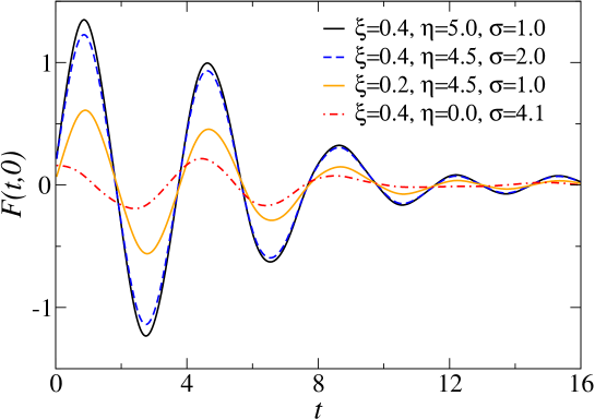
In order to study the effect of the different initial conditions, we show in fig. 6 the time evolution at NLO for $N=8$ and $\lambda=1$, for various choices of initial states with the same energy. The early evolution, $0<t<0.5$, can be understood from the uncoupled case ($\lambda=0$), in which the dynamics is readily solved, and the two-point functions are

$\displaystyle F(t,t^{\prime})=$ $\displaystyle\xi^{2}\cos(mt)\cos(mt^{\prime})+\frac{1}{m^{2}}\left(\eta^{2}+\frac{\sigma^{2}}{4\xi^{2}}\right)\sin(mt)\sin(mt^{\prime})+\frac{\xi\eta}{m}\sin\left[m(t+t^{\prime})\right],$
$\displaystyle\rho(t,t^{\prime})=$ $\displaystyle\frac{\sin\left[m(t-t^{\prime})\right]}{m}.$ (4.11)

The subsequent evolution is of course very different from the free case, in which damping is absent.

Refer to caption

Figure 7: Time evolution of the equal-time correlator $F(t,t)$ for various approximations and the exact result from a numerical solution of the SchrΓΆdinger equation ($N=8$, $\lambda=1$, $\eta=5$, $\xi=0.4$, $\sigma=1$).

Refer to caption

Figure 8: Time evolution of different energy components at N2LOβ€² (same parameters as in fig. 8).

We now continue with a relative large value of $\eta=5$ and a smaller $\xi=0.4$ (corresponding to a squeezed initial state) since this yields an initially large amplitude and subsequent strong damping effects. For the sake of comparison with the numerical solution of the SchrΓΆdinger equation, we consider from now on pure states only, $\sigma=1$.

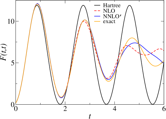
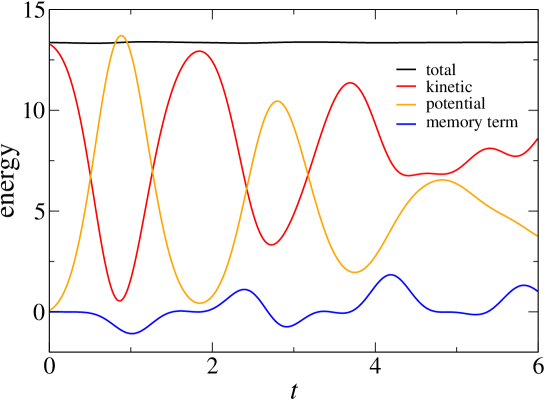
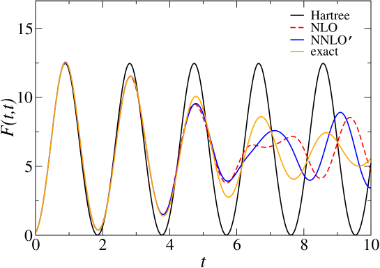
In fig. 8 we show the evolution of the equal-time correlator $F(t,t)$ for the different levels of truncation, at $N=8$. In the Hartree approximation, all nonlocal terms on the RHS of the evolution equations (3.2) are dropped and only the time-dependent mass parameter is preserved. Eqs. (3.4) are dropped altogether. At NLO the one-loop self energies (3.7) without internal vertices are kept. As explained at the end of the previous section, at N2LO we only keep the two-loop self energies, with up to two internal vertices, in addition to the one-loop self energies. We will refer to this truncation as the N2LOβ€² approximation. Since it is derived from the two and three-loop diagrams in fig. 2, it is a 2PI self-consistent approximation. The result labelled with β€˜exact’ corresponds to the numerical solution of the SchrΓΆdinger equation, which is detailed in appendix C. Energy conservation at N2LOβ€² is demonstrated in fig. 8, where the three components in eq. (3.6) and their sum is shown.

A close look at fig. 8 shows that for early times both the NLO and the N2LOβ€² approximation are in quantitative agreement with the exact result. The amplitude in the Hartree approximation shows no sign of decreasing, due to a complete absence of dephasing in quantum mechanics.888This is different in field theory, where the amplitudes of equal-time correlation functions diminish in time due to dephasing. However, in the Hartree approximation the system still experiences recurrence. This shows that damping in the Gaussian approximation is not a result of irreversible loss of memory. Around $t=2.7$, the NLO approximation starts to differ from the exact evolution, whereas the evolution at N2LOβ€² is capable to follow the exact evolution a bit longer. Around $t=4$ we find that both truncations fail to track the exact evolution and continue to evolve in an irregular fashion. We have verified that this behaviour is not due to the time discretisation. We also note that energy remains conserved. The irregular behaviour at later times seems to be peculiar to quantum mechanics and has been observed before in dynamics from truncated effective actions [27]. As far as we know it has not been observed in 2PI dynamics in the field theory case, where already the NLO approximation results in equilibration and thermalization. In this sense quantum mechanics, with only a finite number of degrees of freedom, is very different.

Refer to caption

Figure 9: Same as Figure 8, for $N=2$.

Refer to caption

Figure 10: Same as Figure 8, for $N=20$.

If we continue with a comparison at early times, we note that for $N=8$ the N2LOβ€² approximation works slightly better than the NLO approximation. This can be investigated further by looking at different values for $N$. Since the N2LOβ€² term is suppressed by $1/N$, it is expected that the difference between the N2LOβ€² and the NLO evolution will be largest for smaller $N$, while for larger $N$ the $1/N$ expansion itself is better behaved and the difference between N2LOβ€² and NLO is reduced.

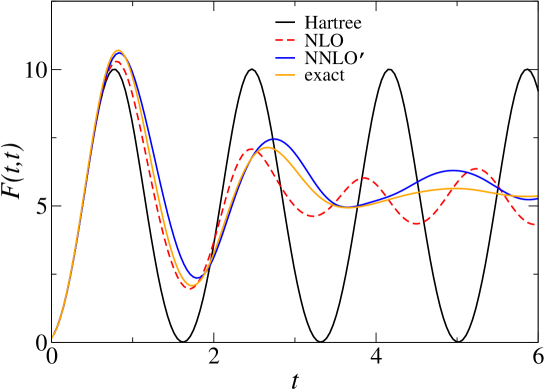
This qualitative picture is confirmed by first going to smaller $N$. In fig. 10 we show again the equal-time correlation function, but now for $N=2$. As expected, the evolution ceases to follow the exact one earlier, but a close look at the first maximum indicates that it is first the Hartree approximation that breaks down, subsequently the NLO approximation and finally the N2LOβ€² approximation. At later times irregular behaviour is again observed. We find therefore that at early times an increase in the order of the truncation has a quantitatively correct effect. In fig. 10 the equal-time correlation function is shown again, but now for larger $N=20$. In this case the effect of adding the N2LOβ€² contribution is much less important, as expected, and we find that the N2LOβ€² evolution follows NLO rather than the exact curve, consistent with an effective convergence of the expansion for large $N$. Both curves follow the exact evolution for longer than in the cases shown above.
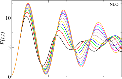
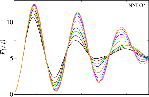
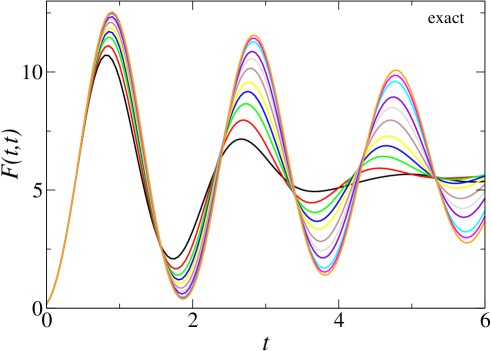
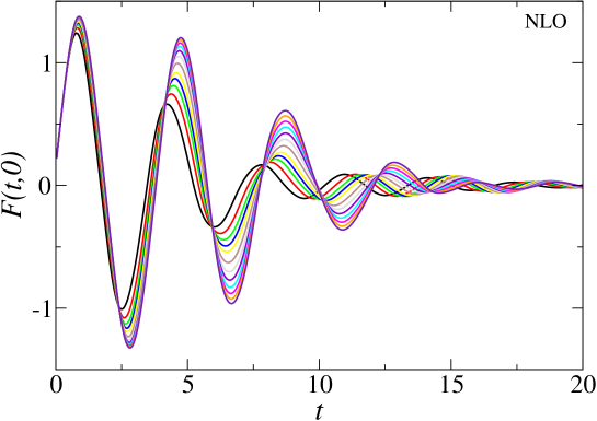
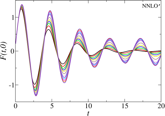
Refer to caption

Refer to caption

Refer to caption

Figure 11: Time evolution of $F(t,t)$ for NLO (upper), N2LOβ€² (middle) and exact (lower) dynamics for various $2\leq N\leq 20$ (other parameters as in fig. 8).

Refer to caption

Refer to caption

Figure 12: Unequal-time correlation function $F(t,0)$ for NLO (upper) and N2LOβ€² (lower) dynamics for various $2\leq N\leq 20$ (other parameters as in fig. 8).

A comparison between the NLO, the N2LOβ€² and the exact evolution is shown in figure 11, for a wide range of $N$, from $N=2$ to $N=20$. It is observed that the exact solution appears to be intermediate between the NLO and N2LOβ€² evolution, with the evolution at N2LOβ€² performing slightly better, in particular in terms of the oscillation frequency at smaller $N$.

As mentioned above, thermalization and equilibration cannot be investigated in quantum mechanics. However, in analogy with field theory effective loss of memory can be studied. In fig. 12 we show the unequal-time two-point function $F(t,0)$ for various values of $N$. Because it is nonlocal in time, this correlator is not immediately accessible from the solution of the SchrΓΆdinger equation. Smaller values of $N$ correspond to a more rapid decrease of the amplitude, as expected. Maybe surprisingly, the memory appears to be washed out faster at NLO than at N2LOβ€² . However, this conclusion should be treated with care, since the approximations fail to track the exact evolution after some ($N$ dependent) time, as was shown above for the equal-time correlation functions.

5 Outlook

We considered nonequilibrium dynamics in the $O(N)$ model, employing the 2PI-$1/N$ expansion to N2LO. We presented the explicit expressions for the three-loop approximation in the auxiliary-field formalism, to which we refer as N2LOβ€², and indicated how to obtain to full N2LO contribution. The resulting evolution equations were solved numerically for quantum mechanics.

While the qualitative change in the nonequilibrium evolution when going from Gaussian (LO) approximations to NLO is enormous, the impact when changing from NLO to N2LO is reassuringly small. This indicates that the 2PI-$1/N$ expansion is effectively rapidly converging and that higher order effects give quantitative corrections only. We found that at early times the evolution at N2LOβ€² performs slightly better than at NLO. This is especially visible at small $N$, where the higher-order contribution is not suppressed. At large times we found that all truncations break down, but we believe that this is special for quantum mechanics since it has not been observed in field theory, where already the NLO approximation has been seen to perform very well. It would therefore be very interesting to implement the N2LO truncation, or at least the three-loop diagram as we considered here, in a $1+1$ dimensional scalar $O(N)$ model and test the apparent convergence quantitatively in field theory, also for late times. Alternatively, with some effort one may also be able to do the full N2LO approximation in the case of quantum mechanics.

Finally, in this paper we only considered the symmetric phase. However, an extension to the broken phase at N2LO is straightforward, since it involves only one additional two-loop diagram in the effective action, yielding new self energy type contributions without internal vertices [17]. In fact, this diagram has been included already in the so-called β€˜bare vertex approximation’ (BVA) [14].

Acknowledgments. G.A. is supported by a PPARC Advanced Fellowship. A.T. is supported by the PPARC SPG β€œClassical Lattice Field Theory”.

Appendix A Loop expansion

Refer to caption

Figure 13: Loop expansion: contribution to $\Gamma_{2}$ up to fifth loop order.

In order to make a connection between the $1/N$ expansion and the ordinary loop expansion (see fig. 13), we give here the expression up to five loops in the loop expansion in the $O(N)$-symmetric case. We write the 2PI contribution as $\Gamma_{2}=\sum_{l=2}^{\infty}\Gamma_{2}^{(l)}$ and find to fourth order

$\displaystyle\Gamma_{2}^{(2)}$ $\displaystyle=$ $\displaystyle-\frac{\lambda}{8}\frac{(N+2)}{3}\int_{x}G^{2}(x,x),$ (A.1)
$\displaystyle\Gamma_{2}^{(3)}$ $\displaystyle=$ $\displaystyle\frac{i\lambda^{2}}{48}\frac{(N+2)}{3N}\int_{xy}G^{4}(x,y),$ (A.2)
$\displaystyle\Gamma_{2}^{(4)}$ $\displaystyle=$ $\displaystyle\frac{\lambda^{3}}{48}\frac{(N+2)(N+8)}{27N^{2}}\int_{xyz}G^{2}(x,y)G^{2}(x,z)G^{2}(z,y).$ (A.3)

At fifth order two diagrams contribute, $\Gamma_{2}^{(5)}=\Gamma_{2}^{(5a)}+\Gamma_{2}^{(5b)}$, which read

$\displaystyle\Gamma_{2}^{(5a)}$ $\displaystyle=$ $\displaystyle-\frac{i\lambda^{4}}{128}\frac{(N+2)(N^{2}+6N+20)}{81N^{3}}\times$ (A.4)
$\displaystyle\int_{xyzw}G^{2}(x,y)G^{2}(y,z)G^{2}(z,w)G^{2}(w,x)$
$\displaystyle\Gamma_{2}^{(5b)}$ $\displaystyle=$ $\displaystyle-\frac{i\lambda^{4}}{32}\frac{(N+2)(5N+22)}{81N^{3}}\times$ (A.5)
$\displaystyle\int_{xyzw}G^{2}(x,y)G(x,z)G(x,w)G^{2}(z,w)G(y,z)G(y,w).$

In the 2PI-$1/N$ expansion to N2LO, $\Gamma_{2}^{(2)}$ and $\Gamma_{2}^{(3)}$ are completely included, while from $\Gamma_{2}^{(4)}$ and $\Gamma_{2}^{(5a)}$ the NLO and N2LO parts are taken into account. The eye diagram $\Gamma_{2}^{(5b)}$ starts at N2LO only. Part of the leading N2LO contribution is taken into account via the three-loop diagram in the auxiliary-field formalism and part via the four-loop diagram. The eye diagram is special since it is the first diagram that contributes to the bulk viscosity in the weak coupling limit [32, 25].

Appendix B Contour integrals

The evolution equations are formulated along the Keldysh contour in the complex-time plane, see fig. 14. Splitting the propagators and self energies in statistical and spectral components yields the real and causal equations discussed in section 3. While for the NLO approximation this procedure is straightforward, it becomes cumbersome when multi-loop contour integrals are encountered and integrals over products of sgn-functions have to be evaluated. Here we give some general expressions we find useful.

Refer to caption

Figure 14: Keldysh contour in the complex-time plane.

First consider integrals over products of $\Theta$-functions. Since the contribution from the upper and lower part of the contour differ only in sign, one finds e.g. that

$$\int_{\cal C}dz^{0}=0,\;\;\;\;\;\;\;\;\;\;\;\;\;\;\;\;\int_{\cal C}dz^{0}\,\Theta_{\cal C}(x,z)=\int_{0}^{x^{0}}dz^{0},$$ (B.1)

or in general

βˆ«π’žπ‘‘z0β€‹βˆi=1MΞ˜π’žβ€‹(xi0,z0)=βˆ‘i=1M[∏jβ‰ iΞ˜π’žβ€‹(xj0,xi0)]β€‹βˆ«0xi0𝑑z0.subscriptπ’ždifferential-dsuperscript𝑧0superscriptsubscriptproduct𝑖1𝑀subscriptΞ˜π’žsuperscriptsubscriptπ‘₯𝑖0superscript𝑧0superscriptsubscript𝑖1𝑀delimited-[]subscriptproduct𝑗𝑖subscriptΞ˜π’žsuperscriptsubscriptπ‘₯𝑗0superscriptsubscriptπ‘₯𝑖0superscriptsubscript0superscriptsubscriptπ‘₯𝑖0differential-dsuperscript𝑧0\int_{\cal C}dz^{0}\prod_{i=1}^{M}\Theta_{\cal C}(x_{i}^{0},z^{0})=\sum_{i=1}^{M}\left[\prod_{j\neq i}\Theta_{\cal C}(x_{j}^{0},x_{i}^{0})\right]\int_{0}^{x_{i}^{0}}dz^{0}. (B.2)

Here we have taken the initial time at $z^{0}=0$. These results can be employed for integrals over products of sgn-functions, using that $\mbox{sgn}_{\cal C}(x,y)=2\Theta_{\cal C}(x,y)-1$, yielding e.g.

$$\int_{\cal C}dz^{0}\,\mbox{sgn}_{\cal C}(x,z)=2\int_{0}^{x^{0}}dz^{0},$$ (B.3)

or in general

βˆ«π’žπ‘‘z0β€‹βˆi=1Msgnπ’žβ€‹(xi0,z0)=2β€‹βˆ‘i=1M[∏jβ‰ isgnπ’žβ€‹(xj0,xi0)]β€‹βˆ«0xi0𝑑z0.subscriptπ’ždifferential-dsuperscript𝑧0superscriptsubscriptproduct𝑖1𝑀subscriptsgnπ’žsuperscriptsubscriptπ‘₯𝑖0superscript𝑧02superscriptsubscript𝑖1𝑀delimited-[]subscriptproduct𝑗𝑖subscriptsgnπ’žsuperscriptsubscriptπ‘₯𝑗0superscriptsubscriptπ‘₯𝑖0superscriptsubscript0superscriptsubscriptπ‘₯𝑖0differential-dsuperscript𝑧0\int_{\cal C}dz^{0}\prod_{i=1}^{M}\mbox{sgn}_{\cal C}(x_{i}^{0},z^{0})=2\sum_{i=1}^{M}\left[\prod_{j\neq i}\mbox{sgn}_{\cal C}(x_{j}^{0},x_{i}^{0})\right]\int_{0}^{x_{i}^{0}}dz^{0}. (B.4)

In a theory with quartic interactions, (B.4) is needed with $M\leq 4$, for which we have verified this identity explicitly.

Appendix C Numerical solution of the SchrΓΆdinger equation

In the case of quantum mechanics, we have the option to solve the SchrΓΆdinger equation numerically for the full wavefunction. This only applies to pure states, $\sigma=1$. The system corresponds to a spherically symmetric anharmonic oscillator in $N$ dimensions, and by imposing $O(N)$ symmetry and make suitable redefinitions we can reduce the problem to that of a particle on a halfline in one dimension [27].

If the wave function is written as the product of a radial function, depending on the (rescaled) radial coordinate $0<r=\sqrt{q_{a}q_{a}/N}<\infty$, and hyperspherical harmonics, depending on the $N-1$ angles,

$$\Psi(q_{a},t)=\left(Nr^{2}\right)^{(N-1)/4}\Phi(r,t)Y(\Omega),$$ (C.1)

the $O(N)$ symmetric problem is reduced to the effective one-dimensional SchrΓΆdinger equation [27]

$$\frac{i}{N}\frac{\partial}{\partial t}\Phi(r,t)={\cal H}_{\rm eff}\Phi(r,t),$$ (C.2)

with the Hamiltonian

$${\cal H}_{\rm eff}=-\frac{1}{2N^{2}}\frac{\partial^{2}}{\partial r^{2}}+U(r),$$ (C.3)

and the effective potential

$$U(r)=\frac{(1-1/N)(1-3/N)}{8r^{2}}+\frac{1}{2}m^{2}r^{2}+\frac{\lambda}{4!}r^{4}.$$ (C.4)

For a pure state the initial radial wave function, corresponding to the density matrix discussed in section 4, is

$$\Phi(r,0)=\frac{1}{\sqrt{\frac{1}{2}\Gamma(N/2)}}\left(\frac{N}{2\xi^{2}}\right)^{N/4}r^{(N-1)/2}\exp\left[-N\left(\frac{1}{4\xi^{2}}+i\frac{\eta}{2\xi}\right)r^{2}\right].$$ (C.5)

This initial wave function is normalized with respect to the innerproduct

⟨Φ|Φ⟩=∫0βˆžπ‘‘r​Φ†​(r,t)​Φ​(r,t).inner-productΦΦsuperscriptsubscript0differential-dπ‘ŸsuperscriptΞ¦β€ π‘Ÿπ‘‘Ξ¦π‘Ÿπ‘‘\langle\Phi|\Phi\rangle=\int_{0}^{\infty}dr\,\Phi^{\dagger}(r,t)\Phi(r,t). (C.6)

We solve eq. (C.2) numerically using the second-order Crank-Nicholson differencing scheme [34]. For the time intervals shown, both unitarity and energy are preserved better than 1 in $10^{12}$.

References

  • [1] For a recent review, see J. Berges, AIP Conf. Proc.  739 (2005) 3 [hep-ph/0409233].
  • [2] J. Zinn-Justin, Quantum Field Theory and Critical Phenomena, Oxford University Press (1989); H. J. de Vega, Commun. Math. Phys.  70 (1979) 29; J. Avan and H. J. de Vega, Phys. Rev. D 29 (1984) 2904.
  • [3] For examples of nonequilibrium quantum field dynamics in the mean-field approximation, see e.g., F. Cooper, S. Habib, Y. Kluger, E. Mottola, J. P. Paz and P. R. Anderson, Phys. Rev. D 50 (1994) 2848 [hep-ph/9405352]; D. Boyanovsky, H. J. de Vega, R. Holman, D. S. Lee and A. Singh, Phys. Rev. D 51 (1995) 4419 [hep-ph/9408214]; D. Boyanovsky, H. J. de Vega, R. Holman and J. F. Salgado, Phys. Rev. D 54 (1996) 7570 [hep-ph/9608205]; D. Boyanovsky, C. Destri, H. J. de Vega, R. Holman and J. Salgado, Phys. Rev. D 57 (1998) 7388 [hep-ph/9711384]; J. Baacke, K. Heitmann and C. PΓ€tzold, Phys. Rev. D 58 (1998) 125013 [hep-ph/9806205], and references therein.
  • [4] L. M. A. Bettencourt and C. Wetterich, Phys. Lett. B 430 (1998) 140 [hep-ph/9712429].
  • [5] G. Aarts, G. F. Bonini and C. Wetterich, Phys. Rev. D 63 (2001) 025012 [hep-ph/0007357].
  • [6] G. Aarts and J. Smit, Phys. Rev. D 61 (2000) 025002 [hep-ph/9906538].
  • [7] M. Salle, J. Smit and J. C. Vink, Phys. Rev. D 64 (2001) 025016 [hep-ph/0012346].
  • [8] L. M. A. Bettencourt, K. Pao and J. G. Sanderson, Phys. Rev. D 65 (2002) 025015 [hep-ph/0104210].
  • [9] J. Berges and J. Cox, Phys. Lett. B 517 (2001) 369 [hep-ph/0006160].
  • [10] G. Aarts and J. Berges, Phys. Rev. D 64 (2001) 105010 [hep-ph/0103049].
  • [11] S. Juchem, W. Cassing and C. Greiner, Phys. Rev. D 69 (2004) 025006 [hep-ph/0307353]; Nucl. Phys. A 743 (2004) 92 [nucl-th/0401046].
  • [12] A. Arrizabalaga, J. Smit and A. Tranberg, Phys. Rev. D 72 (2005) 025014 [hep-ph/0503287].
  • [13] J. Berges, Nucl. Phys. A 699 (2002) 847 [hep-ph/0105311].
  • [14] B. Mihaila, F. Cooper and J. F. Dawson, Phys. Rev. D 63 (2001) 096003 [hep-ph/0006254].
  • [15] G. Aarts and J. Berges, Phys. Rev. Lett.  88 (2002) 041603 [hep-ph/0107129].
  • [16] K. Blagoev, F. Cooper, J. Dawson and B. Mihaila, Phys. Rev. D 64 (2001) 125003 [hep-ph/0106195]; F. Cooper, J. F. Dawson and B. Mihaila, Phys. Rev. D 67 (2003) 051901 [hep-ph/0207346].
  • [17] G. Aarts, D. Ahrensmeier, R. Baier, J. Berges and J. Serreau, Phys. Rev. D 66 (2002) 045008 [hep-ph/0201308].
  • [18] J. Berges and J. Serreau, Phys. Rev. Lett.  91 (2003) 111601 [hep-ph/0208070].
  • [19] F. Cooper, J. F. Dawson and B. Mihaila, Phys. Rev. D 67 (2003) 056003 [hep-ph/0209051].
  • [20] A. Arrizabalaga, J. Smit and A. Tranberg, JHEP 0410 (2004) 017 [hep-ph/0409177].
  • [21] J. Berges, S. BorsΓ‘nyi and J. Serreau, Nucl. Phys. B 660 (2003) 51 [hep-ph/0212404]; J. Berges, S. BorsΓ‘nyi and C. Wetterich, Phys. Rev. Lett.  93 (2004) 142002 [hep-ph/0403234].
  • [22] E. Calzetta and B. L. Hu, Phys. Rev. D 37 (1988) 2878.
  • [23] M. Lindner and M. M. Muller, hep-ph/0512147.
  • [24] J. Berges and S. BorsΓ‘nyi, hep-ph/0512155.
  • [25] E. A. Calzetta, B. L. Hu and S. A. Ramsey, Phys. Rev. D 61 (2000) 125013 [hep-ph/9910334].
  • [26] G. Aarts and J. M. MartΓ­nez Resco, Phys. Rev. D 68 (2003) 085009 [hep-ph/0303216]; JHEP 0402 (2004) 061 [hep-ph/0402192]; JHEP 0503 (2005) 074 [hep-ph/0503161].
  • [27] B. Mihaila, T. Athan, F. Cooper, J. Dawson and S. Habib, Phys. Rev. D 62 (2000) 125015 [hep-ph/0003105]; B. Mihaila, J. F. Dawson, F. Cooper, M. Brewster and S. Habib, hep-ph/9808234.
  • [28] J. Berges and I. O. Stamatescu, Phys. Rev. Lett.  95 (2005) 202003 [hep-lat/0508030].
  • [29] J. M. Cornwall, R. Jackiw and E. Tomboulis, Phys. Rev. D 10 (1974) 2428.
  • [30] S. R. Coleman, R. Jackiw and H. D. Politzer, Phys. Rev. D 10 (1974) 2491.
  • [31] L. F. Abbott, J. S. Kang and H. J. Schnitzer, Phys. Rev. D 13 (1976) 2212.
  • [32] S. Jeon, Phys. Rev. D 52 (1995) 3591 [hep-ph/9409250]; S. Jeon and L. G. Yaffe, Phys. Rev. D 53 (1996) 5799 [hep-ph/9512263].
  • [33] F. Cooper, S. Habib, Y. Kluger and E. Mottola, Phys. Rev. D 55 (1997) 6471 [hep-ph/9610345].
  • [34] W.H. Press, S.A. Teukolsky, W.T. Vetterling and B.P. Flannery, Numerical Recipes in C, Second Edition (Cambridge University Press, United Kingdom).