Rota–Baxter Algebras in Renormalization
of Perturbative Quantum Field Theory

Kurusch Ebrahimi-Fard I.H.É.S. Le Bois-Marie, 35, Route de Chartres,
F-91440 Bures-sur-Yvette, France
kurusch@ihes.fr
   Li Guo Department of Mathematics and Computer Science, Rutgers University,
Newark, NJ 07102
liguo@newark.rutgers.edu
Abstract

Recently, the theory of renormalization in perturbative quantum field theory underwent some exciting new developments. Kreimer discovered an organization of Feynman graphs into combinatorial Hopf algebras. The process of renormalization is captured by a factorization theorem for regularized Hopf algebra characters. In this context the notion of Rota–Baxter algebras enters the scene. We review several aspects of Rota–Baxter algebras as they appear in other sectors also relevant to perturbative renormalization, for instance multiple-zeta-values and matrix differential equations.

   2001 PACS Classification: 03.70.+k, 11.10.Gh, 02.10.Hh, 02.10.Ox

Keywords: Rota–Baxter operators, Atkinson’s theorem, Spitzer’s identity, Baker–Campbell–Hausdorff formula, matrix factorization, renormalization, Hopf algebra of renormalization, Birkhoff decomposition

1 Introduction

In this paper we extend the talk given by one of us (L. G.) at the workshop Renormalization and Universality in Mathematical Physics held at the Fields Institute for Research in Mathematical Sciences, October 18-22, 2005. This talk, as well as the following presentation, is based on our results in [EGK2004, EGK2005, EGGV2006, EG2005b] and explores in detail the algebraic structure underlying the Birkhoff decomposition in the theory of renormalization of perturbative quantum field theory. This decomposition result was discovered by Alain Connes and Dirk Kreimer using the minimal subtraction scheme in dimensional regularization in the context of their Hopf algebraic approach to renormalization [CK2000, CK2001, Krei1998, Krei1999a]. Recently, we extended our findings in joint work with D. Manchon in [EGM2006], presenting a unified picture of several apparently unrelated factorizations arisen from quantum field theory, vertex operator algebras, combinatorics and numerical methods in differential equations.

With a broad range of audience in mind, we summarize briefly some background in perturbative quantum field theory (pQFT) as well as in Hopf algebra and Rota–Baxter algebra, before presenting some of the recent developments. In doing so, we hope to reach a middle ground between mathematics and physics where the algebraic structures which emerged in the work of Connes and Kreimer can be appreciated and further studied by students and researchers in pure and applied areas. For other aspects and more details on the work of Kreimer and collaborators on the Hopf algebra approach to renormalization in pQFT we refer the reader to [EK2005, FG2005, Krei2002, Man2001], as well as the contributions of D. Kreimer and S. Weinzierl in this volume. For readable and brief sources on the basics of renormalization in pQFT using the standard terminology, that is, before the appearance of the more recent Hopf algebra approach, the reader might wish to take a look into J. Gracey’s conference contribution, as well as [Cal1975, CaKe1982], and more recently [Col2006, Del2004]. For a more complete picture on renormalization theory in the context of applications, including calculational details, one should consult the standard textbooks in the field, e.g. [BoSh1959, Col1984, IzZu1980, Muta1987, Vas2004].

The new picture of renormalization in pQFT The very concept of renormalization has a long history [Br1993] going beyond its most famous appearance in perturbative quantum field theory, which started with a short paper on the Lamb shift in perturbative quantum electrodynamics (QED) by H. Bethe [Bet1947]. Eventually, in the context of pQFT, renormalization together with the gauge principle reached the status of a fundamental concept. Its development is marked by contributions by some of the most important figures in 20 century theoretical physics including the founding fathers of pQFT, to wit, Feynman, Dyson, Schwinger, and Tomonaga, see [Kai2005, Schw1994] for more details. Renormalization theory in pQFT reached a satisfying form, from the physics’ point of view, with the formulation known as BPHZ renormalization prescription due to Bogoliubov and Parasiuk [BoPa1957], further improved by Hepp [Hepp1966] and Zimmermann [Zim1969].

As a matter of fact, in most of the interesting and relevant $4$-dimensional quantum field theories, even simple perturbative calculations are plagued with ill-defined, i.e., ultraviolet divergent multidimensional integrals. The removal of these so-called short-distance singularities in a physically and mathematically sound way is the process of renormalization. Although the work of the aforementioned authors played a decisive role in the acceptance of the theory of renormalization in theoretical physics, the conceptual foundation as well as application of renormalization was nevertheless plagued by an ambivalent reputation. Let us cite the following statement from [Del2004], Removing [these] divergencies has been during the decades, the nightmare and the delight of many physicists working in particle physics. [$\dots$] This matter of fact even participated to the nobility of the subject. Moreover, renormalization theory suffered from its lack of a concise mathematical formulation. It was only recently that the foundational, i.e., mathematical structures of renormalization theory in pQFT experienced new and enlightening contributions. These developments started out with the Hopf algebraic formulation of its combinatorial-algebraic structures discovered by Kreimer in [Krei1998] –50 years after Bethe’s paper. This new approach found its satisfying formulation in the work of Connes and Kreimer [CK1998, CK2000, CK2001], and Broadhurst and Kreimer [BK1998, BK1999, BK2000a, BK2000b, BK2001].

In fact, in the Hopf algebra picture the analytic and algebraic aspects of perturbative renormalization nicely decouple, hence making its structure more transparent. The process of renormalization in pQFT finds a surprisingly compact formulation in terms of a classical group theoretical factorization problem. This is one of the main results discovered by Connes and Kreimer in [CK2000, CK2001] using the minimal subtraction scheme in dimensional regularization. It was achieved by first organizing the set $F$ of one-particle irreducible Feynman graphs coming from a perturbative renormalizable QFT (e.g. $\phi^{3}_{6}$, $\phi^{4}_{4}$, QED,…) into a commutative graded connected Hopf algebra ${\mathcal{H}}_{\mathcal{F}}$, where ${\mathcal{F}}:=\mathbb{K}F$ denotes the vector space freely generated by $F$. Its non-cocommutative coproduct map essentially encodes the disentanglement of Feynman graphs into collections of ultraviolet divergent proper one-particle irreducible subgraphs and the corresponding cograph, just as it appears in the original BPHZ prescription, more precisely, Bogoliubov’s ${\bar{\mathrm{R}}}$-map.

Furthermore, regularized Feynman rules seen as linear maps $\phi:{\mathcal{F}}\to A$ from the vector space of graphs into a commutative unital algebra $A$ are extended to $\phi:{\mathcal{H}}_{\mathcal{F}}\to A$ in the group $G_{A}$ of algebra homomorphisms from ${\mathcal{H}}_{\mathcal{F}}$ to $A$. This setting, as we will see, already gives rise to a factorization of such generalized, that is, $A$-valued algebra homomorphisms in the group $G_{A}$. In addition we will observe that when the target space algebra $A$ carries a Rota–Baxter algebra structure, Connes–Kreimer’s Birkhoff decomposition for $G_{A}$ in terms of Bogoliubov’s $\bar{\rm{R}}$-map follows immediately. The last ingredient, i.e. the Rota–Baxter structure is naturally provided by the choice of a renormalization scheme on the regularization space $A$, e.g. minimal subtraction in dimensional regularization.

It was the goal of this talk to present the algebraic underpinning for the result of Connes–Kreimer in terms of a general factorization theorem for complete filtered associative, not necessarily commutative algebras combined with other key results, such as Spitzer’s identity and Atkinson’s theorem for such algebras in the presence of a Rota–Baxter structure.

In fact, we would like to show how the above factorization problem for renormalization may be formulated more transparently as a classical decomposition problem for matrix Lie groups. This is achieved by establishing a representation of the group of regularized Hopf algebra characters by –infinite dimensional– unipotent lower triangular matrices with entries in a commutative unital Rota–Baxter algebra. The representation space is given by –a well-chosen vector subspace of– the vector space ${\mathcal{F}}$ of 1PI Feynman graphs corresponding to the pQFT. The demand for entries in a commutative Rota–Baxter algebra induces a non-commutative Rota–Baxter structure on the underlying matrix algebra such that Spitzer’s theorem applies, and indeed, as we will see, this paves smoothly the way to Bogoliubov’s $\bar{\mathrm{R}}$-map, though in matrix form.

Before giving a more detailed account on this purely algebraic structure we should underline that the initial proof of the Connes–Kreimer factorization of regularized Feynman rules was achieved using dimensional regularization, i.e., assuming $A$ to be the field of Laurent series, hereby opening a hitherto hidden geometric viewpoint on perturbative renormalization in terms of a correspondence to the Riemann–Hilbert problem. For the minimal subtraction scheme it amounts to the multiplicative decomposition of the Laurent series associated to a Feynman graph using dimensionally regularized Feynman rules. Such a Laurent series has poles of finite order in the regulator parameter and the decomposition happens to be the one into a part holomorphic at the origin and a part holomorphic at the complex infinity. The latter moreover distinguishes itself by the particular property of locality. This has far reaching geometric implications, starting with the interpretation upon considering the Birkhoff decomposition of a loop around the origin, providing the clutching data for the two half-spheres defined by that very loop. Connes and Kreimer found a scattering type formula for the part holomorphic at complex infinity, that is, the counterterm, giving rise to its description in terms of iterated integrals.

Moreover, by some recent progress, which has been made in the mathematical context of number theory, and motivic aspects of Feynman integrals, this geometric point of view leads to motivic Galois theory upon studying the notion of equisingular connections in the related Riemann–Hilbert correspondence. This was used to explore Tannakian categories and Galois symmetries in the spirit of differential Galois theory in [CM2004a, CM2006, CM2004b]. Underlying the notion of an equisingular connection is the locality of counterterms, which itself results from Hochschild cohomology. The resulting Dyson–Schwinger equation allows for gradings similar to the weight- and Hodge filtrations for the polylogarithm [Krei2003a, Krei2004]. More concretely, the motivic nature of primitive graphs has been established very recently by Bloch, Esnault and Kreimer in [BEK2005].

We now outline the organization of the paper. In Section 2 we review some pieces from renormalization theory in pQFT up to the introduction of Bogoliubov’s $\bar{\mathrm{R}}$-map. We use Section 3 for introducing most of the basic mathematical notions needed in the sequel, especially with respect to Hopf algebras. A general factorization theorem for complete filtered algebras is presented, based on a new type of recursion equation defined in terms of the Baker–Campbell–Hausdorff ($BC\!H$) formula. We establish Connes’ and Kreimer’s Hopf respectively Lie algebra of Feynman graphs as well as their Birkhoff decomposition of regularized Hopf algebra characters. Section 4 is devoted to a not-so-short review of the concept of Rota–Baxter algebra, including a list of instructive examples as well as Spitzer’s identity and a link between the Magnus recursion known from matrix differential equations and the new $BC\!H$-recursion. Section 5 contains a presentation of the Rota–Baxter algebra structure underlying the Birkhoff decomposition of Connes–Kreimer. We establish a matrix representation of the group of regularized Feynman rules characters and recover Connes–Kreimer’s Birkhoff decomposition in terms of a classical matrix factorization problem.

2 Renormalization in pQFT: Bogoliubov’s $\bar{\mathrm{R}}$-operation

We recall some of the essential points from classical renormalization theory as applied in the context of pQFT. We follow Kreimer’s book [Krei2000] and the recent brief and concise summary given by Collins in [Col2006].

2.1 Feynman rules and renormalizability

Let us begin with a statement which summarizes perturbative renormalization theory of QFT in its Lagrangian formulation. The quintessence of –multiplicative– renormalization says that under the severe constraint of maintaining the physical principles of locality, unitarity, and Lorentz invariance, it is possible to absorb to all orders in perturbation theory the (ultraviolet) divergencies in a redefinition of the parameters defining the QFT. Here, in fact, two very distinct concepts enter, to wit, that of renormalizability, and the process of renormalization. The former distinguishes those theories with only a finite number of parameters, lending them considerably more predictive power. However, the process of renormalization instead works order by order, indifferently of the number of parameters.

In the Lagrangian picture we start with a Lagrangian density defining the QFT, which we assume to be renormalizable. For instance, the so-called $\phi^{4}$ and $\phi^{3}$ theories are described by the following two Lagrangians

$$L=\frac{1}{2}(\partial_{\mu}\phi)^{2}-\frac{1}{2}m_{1}^{2}\phi^{2}+\frac{\lambda_{4}}{4!}\phi^{4}\quad{\makebox{ resp. }}\qquad L=\frac{1}{2}(\partial_{\mu}\phi)^{2}-\frac{1}{2}m_{2}^{2}\phi^{2}+\frac{\lambda_{3}}{3!}\phi^{3}.$$

The classical calculus of variations applied to $L=\frac{1}{2}(\partial_{\mu}\phi)^{2}-\frac{1}{2}m_{i}^{2}\phi^{2}$, $i=1,2$ provides the equations of motion

$$\partial_{\mu}\frac{\delta L}{\delta\partial_{\mu}\phi}-\frac{\delta L}{\delta\phi}=0\Rightarrow\;(\Box+m_{i}^{2})\phi(x)=0,\qquad i=1,2.$$

There is only one type of –scalar– field denoted by $\phi=\phi(x)$, parametrized by the $D$ dimensional space-time point $x=(t,{\bf{x}})$. The parameters $m_{1},m_{2}$ and $\lambda_{4},\lambda_{3}$ are called the mass and coupling constants, respectively. The equations of motion as well as the Lagrangian are local in the sense that all fields are evaluated at the same space-time point. The reader interested in quantum field theories more relevant to physics, such as QED or quantum chromodynamics, should consult the standard literature, for instance [BoSh1959, Col1984, IzZu1980, Muta1987, Ryd1985, tHVel1973].

We may separate the above Lagrangians into a free and an interaction part, $L=L_{f}+L_{i}$, where in the both cases above $L_{f}=\frac{1}{2}(\partial_{\mu}\phi)^{2}-\frac{1}{2}m_{i}^{2}\phi^{2}$, $i=1,2$. The remaining quartic respectively cubic term represents the interaction part, $L_{i}$.

The general goal is to calculate the $n$-point Green’s functions,

$$G(x_{1},\ldots,x_{n}):=\langle 0|{\rm{T}}[\phi(x_{1})\cdots\phi(x_{n})]|0\rangle$$

where the time-ordering ${\rm{T}}$-operator is defined by

$\displaystyle{\rm{T}}[\phi(x_{1})\phi(x_{2})]:=\begin{cases}\phi(x_{1})\phi(x_{2}),\ {\rm{if}}\ t_{1}>t_{2},\\ \phi(x_{2})\phi(x_{1}),\ {\rm{if}}\ t_{2}>t_{1},\end{cases}$

since from these vacuum correlators of time-ordered products of fields one can obtain all $S$-matrix elements with the help of the LSZ-formalism, see for instance [IzZu1980] for more details.

So far, perturbation theory is the most successful approach to Lagrangian QFT with an overwhelming accordance between experimental and theoretical, that is, perturbative results.

In perturbation theory Green’s functions are expanded in power series of a supposed to be small parameter like the coupling constant (or Planck’s $\hbar$). Its coefficients are given by complicated iterated integrals of the external parameters defining the scattering process, respectively the participating particles. However, these coefficients turn out to show a highly organized structure. Indeed, Feynman discovered a graphical coding of such expressions in terms of graphs that later bore his name. A Feynman graph is a collection of internal and external lines, or edges, and vertices of several types. Proper subgraphs of a Feynman graph are determined by proper subsets of the set of internal edges and vertices.

Eventually, perturbative expansions in QFT are organized in terms of one-particle irreducible (1PI) Feynman graphs, i.e., connected graphs that stay connected upon removal of any of the internal edges, also called propagators. For example, we have such simple drawings as  or encoding Feynman amplitude integrals appearing in the expansion of the $4$-point Green’s function in $\phi^{4}$-theory. The fact that there is only one type of –undirected– lines and only $4$-valent vertices reflects the fact that the Lagrangian $L$ only contains one type of –scalar– field $\phi$ with only a quartic interaction term in $L_{i}$. For the $\phi^{3}$ case we would find drawings with only $3$-valent vertices and one type of undirected lines.

Feynman rules give a mean to translate these drawings –back– into the corresponding amplitudes. The goal is to calculate them order by order in the coupling constants of the theory. Originally, a graph was somehow ‘identified’ with its amplitude. Let us remark that it is only in the Hopf algebraic picture that these objects get properly distinguished into the algebraic-combinatorial and analytic side of the same underlying pQFT picture. We will see that in this context graphs are studied as combinatorial objects organized into (pre-)Lie algebras and the corresponding Hopf algebras. Whereas Feynman rules provide particular maps assigning analytic expressions, the so-called Feynman amplitudes, to these graphs.

As an example for the latter we list here the set of Feynman rules related to the above Lagrangian of the $\phi^{4}$-theory in four space-time dimensions [Krei2000].

  • For each internal scalar field line, associate a propagator: $i\Delta(p)=\frac{i}{p^{2}-m^{2}+i\eta}$.

  • At each vertex require momentum conservation and place a factor of $-i\lambda_{4}$.

  • For each closed loop in the graph, integrate over $\int\frac{d^{4}q}{(2\pi)^{4}},$ where $q$ is the momentum associated with the loop.

  • For any Feynman graph $\Gamma$ built from these propagators and vertices divide by the symmetry factor $sym(\Gamma)$ of the graph, which is assumed to contain $r$ vertices. The symmetry factor is then given by the number of possibilities to connect $r$ vertices to give $\Gamma$, divided by $(4!)^{r}$.

A few examples are presented now, see for instance [FG2005] and the standard literature. Let us write down the integral expression corresponding to the graph called fish, , made out of two $4$-valent vertices and two propagators. The unconnected vertex legs carry the external momenta of the in- and outgoing particles which are denoted by $k_{1},k_{2},k_{3},k_{4}$. They are related by a delta function ensuring the overall momentum conservation.

I():=(iλ4)2d4q(2π)4i(q+k1+k2)2m2+iηiq2m2+iη.assign𝐼superscript𝑖subscript𝜆42superscript𝑑4𝑞superscript2𝜋4𝑖superscript𝑞subscript𝑘1subscript𝑘22superscript𝑚2𝑖𝜂𝑖superscript𝑞2superscript𝑚2𝑖𝜂I(\parbox{18.0pt}{\begin{picture}(10.0,10.0)\put(1.0,5.0){\qbezier(0.0,-2.0)(8.0,10.0)(16.0,-2.0)} \put(1.0,5.0){\qbezier(0.0,2.0)(8.0,-10.0)(16.0,2.0)} \end{picture}}):=\left(-i\lambda_{4}\right)^{2}\int\frac{d^{4}q}{(2\pi)^{4}}\frac{i}{(q+k_{1}+k_{2})^{2}-m^{2}+i\eta}\ \frac{i}{q^{2}-m^{2}+i\eta}. (1)

For the bikini graph,  , with three $4$-valent vertices and four propagators we find after some algebra a product of two ‘fishy’ integrals

I()𝐼\displaystyle I(\parbox{24.0pt}{\begin{picture}(10.0,5.0)\put(0.0,2.0){\qbezier(0.0,-1.5)(6.0,7.5)(11.4,0.0)} \put(0.0,2.0){\qbezier(0.0,1.5)(6.0,-7.5)(11.4,0.0)} \put(10.8,2.0){\qbezier(0.6,0.0)(6.0,7.5)(12.0,-1.5)} \put(10.8,2.0){\qbezier(0.6,0.0)(6.0,-7.5)(12.0,1.5)} \end{picture}}) $\displaystyle:=$ $\displaystyle\left(-i\lambda_{4}\right)^{3}\int\frac{d^{4}q}{(2\pi)^{4}}\frac{i}{(q+k_{1}+k_{2})^{2}-m^{2}+i\eta}\ \frac{i}{q^{2}-m^{2}+i\eta}\times$ (2)
$\displaystyle\qquad\quad\int\frac{d^{4}p}{(2\pi)^{4}}\frac{i}{(p+k_{1}+k_{2})^{2}-m^{2}+i\eta}\ \frac{i}{p^{2}-m^{2}+i\eta}.$

Let us go one step further and write down the integral for the winecup graph,  , of order three in the coupling constant $i\lambda_{4}$, also made out of four propagators

I()𝐼\displaystyle I\big{(}\parbox{16.79993pt}{\begin{picture}(10.0,10.0)\put(5.9,-1.4){\line(2,3){9.0}} \put(11.1,-1.4){\line(-2,3){9.0}} \put(4.0,7.5){\qbezier(0.0,1.8)(4.5,5.0)(9.0,1.8)} \put(4.0,7.5){\qbezier(0.0,1.8)(4.5,-1.25)(9.0,1.8)} \end{picture}}\big{)} $\displaystyle:=$ $\displaystyle\left(-i\lambda_{4}\right)^{3}\int\frac{d^{4}p}{(2\pi)^{4}}\ \int\frac{d^{4}q}{(2\pi)^{4}}\frac{i}{(q+k_{1}+k_{2})^{2}-m^{2}+i\eta}\ \frac{i}{q^{2}-m^{2}+i\eta}\times$ (3)
$\displaystyle\qquad\qquad\qquad\qquad\frac{i}{(q^{2}-m^{2}+i\eta)\ ((p-q-k_{3})^{2}-m^{2}+i\eta)}.$

Unfortunately, all of the above integrations over the loop-momenta are not restricted by any constraint and some power-counting analysis of the integrands reveals a serious problem as we observe that the above integrals are not well-defined for high loop-momenta.

For the purpose of classifying such problematic integrals within a pQFT, we must introduce the notion of superficial degree of divergence associated to a Feynman graph $\Gamma$ and denoted by $\omega(\Gamma)$. In general, $\omega(\Gamma)$ simply follows from counting powers of integral loop-momenta in the corresponding Feynman integral in the limit when they are large. The amplitude corresponding to the graph $\Gamma$ is superficially convergent if $\omega(\Gamma)<0$, and superficially divergent for $\omega(\Gamma)\geq 0$. For $\omega(\Gamma)=0$ we call the diagram superficially logarithmically divergent and we say that it is superficially linearly divergent, if $\omega(\Gamma)=1$. No doubt, we may continue this nomenclature. Superficially here reflects the very fact that the integral associated to a graph might appear to be convergent, but due to ill-defined subintegrals corresponding to ultraviolet divergent 1PI subgraphs it is divergent in fact.

Restricting ourselves to scalar theories such as the two examples at the beginning one can derive a simple expression for $\omega(\Gamma)$ depending on the structure of the graph, i.e., its vertices and edges, as well as the space-time dimension. We assume a Lagrangian of the general form $L=L_{f}+\sum_{k=3}L_{i_{k}}$ where $L_{f}$ as usual consists of the free part and the sum contains the interaction field monomials of the form $L_{i_{k}}:=\frac{\lambda_{k}}{k!}\phi^{k}$. Recall that the canonical dimension (inverse length) in $D$ space-time dimensions of the scalar field $\phi$ is given by $[\phi]=(D-2)/2$ in natural units, following from the free part of the Lagrangian. Therefore we have $[\phi^{k}]=(D-2)k/2=:\omega_{k}$ and the coupling constant must be of dimension $[\lambda_{k}]=D-\omega_{k}$.

For a given connected graph $\Gamma$ consisting of $E=E(\Gamma)$ external lines, $I=I(\Gamma)$ internal lines and $V=V(\Gamma)$ vertices we find $L=I-V+1$ loop integrations in the corresponding amplitude. By standard considerations it follows that $E-2I=\sum_{j=1}^{V}n_{j}$, where $n_{j}$ denotes the order, or valency, of the $j$-th vertex in $\Gamma$. Since each $D$ dimensional loop integration contributes $D$ loop momenta in the numerator and each propagator contributes two inverse loop momenta it follows that

$$\omega(\Gamma)=DL-2I=D-\frac{D-2}{2}E+\sum_{j=1}^{V}\Big{(}\frac{D-2}{2}n_{j}-D\Big{)}.$$

The last term is just $\frac{D-2}{2}n_{j}-D=\omega_{n_{j}}-D=[\lambda_{n_{j}}]$ and hence

$$\omega(\Gamma)=D-\frac{D-2}{2}E+\sum_{j=1}^{V}[\lambda_{n_{j}}].$$

For our $\phi^{4}$-theory in $D=4$ space-time dimensions we find a dimensionless coupling constant, $[\lambda_{4}]=0$, which implies $\omega(\Gamma)=4-E$. In fact, from this formula it follows immediately that the above integrals are all superficially logarithmically divergent, rendering the perturbative series expansion of –the $4$-point– Green’s functions quite useless right from the start, to wit, for the $1$-loop fish diagram  corresponding to the first non-trivial term in the perturbation expansion of the $4$-point Green’s functions in $D=4$ space-time dimensions we find ω()=D4=44=0𝜔𝐷4440\omega(\parbox{18.0pt}{\begin{picture}(10.0,10.0)\put(1.0,5.0){\qbezier(0.0,-2.0)(8.0,10.0)(16.0,-2.0)} \put(1.0,5.0){\qbezier(0.0,2.0)(8.0,-10.0)(16.0,2.0)} \end{picture}})=D-4=4-4=0, which indicates the existence of a so-called logarithmic ultraviolet (UV) divergence. The reader is referred to the literature for more details on the related dimensional analysis of pQFT revealing the role played by the number of space-time dimensions and the related classification into non-renormalizable, (just) renormalizable and super-renormalizable theories [Cole1988, IzZu1980, PS1995, Ryd1985]. Let us mention that in the $\phi^{4}$ example the number of $D=4$ space-time dimensions just happens to be the critical one, and that we would make a similar observation for the Lagrangian with cubic interaction in $D=6$ space-time dimensions.

At this level and under the assumption that the perturbative QFT is renormalizable, the programm of –multiplicative– renormalization enters the stage. Its non-trivial operations will cure the ultraviolet deficiencies in a self-consistent and physically sound way order by order in the series expansion.

2.2 Multiplicative renormalization

The machinery of multiplicative renormalization consists of the following parts.

Regularization: first, one must regularize the theory, rendering integrals of the above type formally finite upon the introduction of new and nonphysical parameters. For instance, one might truncate, i.e., cut-off the integration limits at an upper bound $\Lambda$ by introducing a step-function $\Theta$

$$\int d^{4}q\frac{\Theta[\Lambda-q^{2}]}{(q+k_{1}+k_{2})^{2}-m^{2}+i\eta}\frac{1}{q^{2}-m^{2}+i\eta}.$$

Evaluating such an integral results in $\log$-terms containing $\Lambda$ so that naively removing the cut-off parameter by taking the limit $\Lambda\to\infty$ must be avoided since it gives back the original divergence. The cut-off approach usually interferes with gauge symmetry.

Another regularization scheme is dimensional regularization [Col1984, tH1973], which respects –almost– all symmetries of the theory under consideration. It introduces a complex parameter by changing the integral measure, that is, the space-time dimension $D\in\mathbb{N}$ to $\mathcal{D}\in\mathbb{C}$

$$\frac{d^{D}q}{(2\pi)^{D}}\longrightarrow\mu^{2\varepsilon}\frac{d^{\mathcal{D}}q}{(2\pi)^{\mathcal{D}}},$$

where $\varepsilon=\frac{(D-{\mathcal{D}})}{2}\in\mathbb{C}$. The parameter $\mu$ (t’Hooft’s mass) is introduced for dimensional reasons. Hence, forgetting about the other involved variables, that do not enter our considerations, dimensionally regularized Feynman rules associate to each graph an element from the field of Laurent series $\mathbb{C}[\varepsilon^{-1},\varepsilon]]$. In general, one obtains a proper Laurent series of degree at most $n$ in an $n$-loop calculation, which means that we have at most poles of order $n$ in the regularized Feynman integral corresponding to a graph with $n$ independent closed cycles. The pole terms parametrize the UV-deficiency of the integrals. Obviously, the limit of $\varepsilon\to 0$ results in the original divergences of the integral and must be postponed.

Let us emphasize that it is common knowledge that the choice of the regularization procedure is highly arbitrary and mainly driven by calculational conveniences and the wish to conserve symmetries of the original theory.

But, so far we have not achieved much more than a parametrization of the divergent structure of Feynman integrals. Though important and useful all this just indicates the need of some more sophisticated set of rules on how to handle the terms which diverge with $\Lambda\to\infty$ in the cut-off setting respectively $\varepsilon\to 0$ for dimensional regularization, since in the end we must remove these non-physical regularization parameters.

Renormalization: to render the picture complete we must fix a so-called renormalization scheme (or condition), which is supposed to isolate the divergent part of a regularized integral. For instance, in dimensional regularization a natural choice is the minimal subtraction scheme $R:=R_{ms}$, mapping a Laurent series to its strict pole part, i.e., $R\big{(}\sum_{n\geq-N}a_{n}\varepsilon^{n}\big{)}:=\sum_{n=-N}^{-1}a_{n}\varepsilon^{n}$.

The next and conceptually most demanding step is to provide a procedure which renders the integrals finite upon the removal of the regularization parameters order by order in a –mathematically and– physically sound way. This actually goes along with the proof of perturbative renormalizability of the underlying QFT. A convenient procedure which accomplishes this and which is commonly used nowadays was established by Bogoliubov and Parasiuk, further improved by Hepp and Zimmermann.

Let us go back to the statement we made at the beginning of this section, characterizing the concept of perturbative renormalization in a –renormalizable– QFT. The idea is to redefine multiplicatively the parameters appearing in the Lagrangian $L$ so as to absorb all divergent contributions order by order in the perturbation expansion. We will outline this idea in the next step where we briefly indicate how to implement Bogoliubov’s subtraction procedure for renormalization in a multiplicative way on the level of the Lagrangian by adding the so-called counterterm Lagrangian $L_{c}$ to the original Lagrangian $L=L_{f}+L_{i}$. Indeed, the result is $L\xrightarrow{ren.}L_{ren}=L+L_{c}$ with $L_{ren}$ describing the perturbatively renormalized quantum field theory. We achieve this by introducing so-called $\mathrm{Z}$-factors together with the idea of renormalized respectively bare parameters. In the case of the $\phi^{4}$-theory we have

$$L_{ren}=L_{f}+L_{i}+\underbrace{\frac{Z_{\phi}-1}{2}(\partial_{\mu}\phi)^{2}-\frac{(m_{1}^{2}Z_{m_{1}}-m_{1}^{2})}{2}\phi^{2}+\frac{(\lambda_{4}Z_{\lambda_{4}}-\lambda_{4})}{4!}\phi^{4}}_{L_{c}}.$$

One can reorganize the right hand side into the original form upon introducing the notion of bare fields and bare parameters. First, we replace the field $\phi$ by the bare field

$$\phi_{0}:=Z_{\phi}^{\frac{1}{2}}\phi$$

defined in terms of the $\mathrm{Z}$-factor $Z_{\phi}:=1+\delta\phi$. Then, we introduce the $\mathrm{Z}$-factors $Z_{m_{1}}$, $Z_{\lambda_{4}}$ and replace the parameters $m_{1}$ and $\lambda_{4}$ by bare parameters

$$m^{2}_{1,0}:=m_{1}^{2}Z_{m_{1}}Z^{-1}_{\phi}=m^{2}_{1}\frac{(1+\delta m_{1})}{(1+\delta\phi)},\makebox{ and }\ \lambda_{4,0}:=\lambda_{4}Z_{\lambda_{4}}Z^{-2}_{\phi}=\lambda_{4}\frac{(1+\delta\lambda_{4})}{(1+\delta\phi)^{2}},$$

such that we can write the multiplicatively renormalized Lagrangian as

$$L_{ren}=\frac{1}{2}(\partial_{\mu}\phi_{0})^{2}-\frac{1}{2}m_{1,0}^{2}\phi_{0}^{2}+\frac{\lambda_{4,0}}{4!}\phi_{0}^{4}.$$

The property of the original $\phi^{4}$ Lagrangian, $L=L_{f}+L_{i}$, to be renormalizable is encoded in the fact that the counterterm Lagrangian, $L_{c}$, only contains field monomials which also appear in $L$. This allows us to recover $L_{ren}$ in the original form of $L$ upon introducing bare parameters respectively the $\mathrm{Z}$-factors, which implies the notion of multiplicative renormalization. We observe explicitly that $Z_{\phi}$ must be a numerical constant to assure locality ($[Z_{\phi},\partial_{\mu}]=0$). This is also true for the other $\mathrm{Z}$-factors as well. However, they depend in a highly singular form on the regularization parameter. In fact, $Z_{X}=1+\delta X$ is an order by order determined infinite power series of counterterms, each of which is divergent when removing the regulator parameter. They are introduced to compensate –i.e. renormalize– the pole parts in the original perturbation expansion, and –one must prove that– such a process assures the cancellation of divergent contributions at each order in perturbation theory, see e.g. [Col1984, IzZu1980].

2.3 Preparation of Feynman graphs for simple subtraction

Recall that a proper connected UV divergent 1PI subgraph $\gamma$ of a 1PI Feynman graph $\Gamma$ is determined by proper subsets of the set of internal edges and vertices of $\Gamma$.

Bogoliubov’s $\bar{\mathrm{R}}$-operation provides a recursive way to calculate the counterterms, which we mentioned above and denoted by $C(\Gamma)$ for each Feynman graph $\Gamma$ as follows. The $\bar{\mathrm{R}}$-operation maps a graph $\Gamma$, that is, the corresponding regularized amplitude to a linear combination of suitably modified graphs including $\Gamma$ itself

$$\bar{\mathrm{R}}(\Gamma):=\Gamma+\sum\!{}^{\prime}_{\{\gamma{}^{\prime}\}\subsetneq\Gamma}\Gamma\big{(}\{\gamma{}^{\prime}\}\to C(\gamma{}^{\prime})\big{)}.$$ (4)

We follow the notation of [Col2006]. The primed sum is over all unions $\{\gamma{}^{\prime}\}$ of UV divergent 1PI subgraphs sitting inside $\Gamma$. More concretely, following the terminology used in [CaKe1982] we call $\mathfrak{s}:=\{\gamma{}^{\prime}\}$ a proper spinney of $\Gamma$ if it consists of a nonempty union of disjoint proper UV divergent 1PI subgraphs, $\{\gamma{}^{\prime}\}:=\{\gamma^{\prime}_{1}\dots\gamma^{\prime}_{n}\}$, $\gamma^{\prime}_{i}\subsetneq\Gamma$, $\gamma^{\prime}_{i}\cap\gamma^{\prime}_{j}=\emptyset$ for $i\neq j$. We call the union of all such spinneys in the graph $\Gamma$ a proper wood which we denote by

$$\mathfrak{W}(\Gamma):=\big{\{}\{\gamma{}^{\prime}\}\subsetneq\Gamma\ \big{|}\{\gamma{}^{\prime}\}=\{\mathrm{union\ of\ disjoint\ proper\ 1PI\ subgraphs}\}\big{\}}.$$

Let us enlarge this set to $\bar{\mathfrak{W}}(\Gamma)$ which includes by definition the empty set, $\{\emptyset\}$, and the graph $\{\Gamma\}$ itself, i.e., $\{\emptyset\},\{\Gamma\}\in\bar{\mathfrak{W}}(\Gamma)$.

For instance, the two loop self-energy graph Γ=\SetWidth3.0 \SetColorBlack \Line(105,-60)(240,-135) \Line(375,-60)(450,-60) \Line(240,-135)(240,15) \Line(375,-60)(240,-135) \Line(105,-60)(240,15) \Line(30,-60)(105,-60) \Line(240,15)(375,-60) Γ\SetWidth3.0 \SetColorBlack \Line(105,-60)(240,-135) \Line(375,-60)(450,-60) \Line(240,-135)(240,15) \Line(375,-60)(240,-135) \Line(105,-60)(240,15) \Line(30,-60)(105,-60) \Line(240,15)(375,-60) \Gamma\!=\!\!\begin{array}[]{c}\scalebox{0.6}{{\scalebox{0.13}{ \begin{picture}(420.0,150.0)(30.0,-135.0)\SetWidth{3.0} \SetColor{Black} \Line(105,-60)(240,-135) \Line(375,-60)(450,-60) \Line(240,-135)(240,15) \Line(375,-60)(240,-135) \Line(105,-60)(240,15) \Line(30,-60)(105,-60) \Line(240,15)(375,-60) \end{picture}}}}\\ \end{array}, borrowed from $\phi^{3}$-theory in six dimensions, has two proper 1PI UV subgraphs γl=\SetWidth3.0 \SetColorBlack \Line(105,-60)(255,-135) \Line(105,-60)(255,15) \Line(225,-115)(225,-4) \Line(60,-60)(105,-60) subscript𝛾𝑙\SetWidth3.0 \SetColorBlack \Line(105,-60)(255,-135) \Line(105,-60)(255,15) \Line(225,-115)(225,-4) \Line(60,-60)(105,-60) \gamma_{l}\!=\!\!\begin{array}[]{c}\scalebox{0.6}{{\scalebox{0.13}{ \begin{picture}(195.0,150.0)(60.0,-135.0)\SetWidth{3.0} \SetColor{Black} \Line(105,-60)(255,-135) \Line(105,-60)(255,15) \Line(225,-115)(225,-4) \Line(60,-60)(105,-60) \end{picture}}}}\\ \end{array} and γr=\SetWidth3.0 \SetColorBlack \Line(135,-135)(285,-60) \Line(135,15)(285,-60) \Line(330,-60)(285,-60) \Line(165,-115)(165,-1) subscript𝛾𝑟\SetWidth3.0 \SetColorBlack \Line(135,-135)(285,-60) \Line(135,15)(285,-60) \Line(330,-60)(285,-60) \Line(165,-115)(165,-1) \gamma_{r}\!=\!\!\begin{array}[]{c}\scalebox{0.6}{{\scalebox{0.13}{ \begin{picture}(195.0,150.0)(135.0,-135.0)\SetWidth{3.0} \SetColor{Black} \Line(135,-135)(285,-60) \Line(135,15)(285,-60) \Line(330,-60)(285,-60) \Line(165,-115)(165,-1) \end{picture}}}}\\ \end{array}, but they are not disjoint. Instead, they happen to be overlapping, i.e. $\gamma_{r}\cap\gamma_{l}\neq\emptyset$ in $\Gamma$. This is why we do not have $\{\gamma_{l}\ \gamma_{r}\}\notin\mathfrak{W}(\Gamma)$, that is, the set of proper spinneys corresponding to that graph is

𝔚(\SetWidth3.0 \SetColorBlack \Line(105,-60)(240,-135) \Line(375,-60)(450,-60) \Line(240,-135)(240,15) \Line(375,-60)(240,-135) \Line(105,-60)(240,15) \Line(30,-60)(105,-60) \Line(240,15)(375,-60) )={{\SetWidth3.0 \SetColorBlack \Line(135,-135)(285,-60) \Line(135,15)(285,-60) \Line(330,-60)(285,-60) \Line(165,-115)(165,-1) },{\SetWidth3.0 \SetColorBlack \Line(105,-60)(255,-135) \Line(105,-60)(255,15) \Line(225,-115)(225,-4) \Line(60,-60)(105,-60) }}.𝔚\SetWidth3.0 \SetColorBlack \Line(105,-60)(240,-135) \Line(375,-60)(450,-60) \Line(240,-135)(240,15) \Line(375,-60)(240,-135) \Line(105,-60)(240,15) \Line(30,-60)(105,-60) \Line(240,15)(375,-60) \SetWidth3.0 \SetColorBlack \Line(135,-135)(285,-60) \Line(135,15)(285,-60) \Line(330,-60)(285,-60) \Line(165,-115)(165,-1) \SetWidth3.0 \SetColorBlack \Line(105,-60)(255,-135) \Line(105,-60)(255,15) \Line(225,-115)(225,-4) \Line(60,-60)(105,-60) \mathfrak{W}\Big{(}\!\!\begin{array}[]{c}\scalebox{0.6}{{\scalebox{0.13}{ \begin{picture}(420.0,150.0)(30.0,-135.0)\SetWidth{3.0} \SetColor{Black} \Line(105,-60)(240,-135) \Line(375,-60)(450,-60) \Line(240,-135)(240,15) \Line(375,-60)(240,-135) \Line(105,-60)(240,15) \Line(30,-60)(105,-60) \Line(240,15)(375,-60) \end{picture}}}}\\ \end{array}\!\!\Big{)}=\Big{\{}\big{\{}\!\!\begin{array}[]{c}\scalebox{0.6}{{\scalebox{0.13}{ \begin{picture}(195.0,150.0)(135.0,-135.0)\SetWidth{3.0} \SetColor{Black} \Line(135,-135)(285,-60) \Line(135,15)(285,-60) \Line(330,-60)(285,-60) \Line(165,-115)(165,-1) \end{picture}}}}\\ \end{array}\!\!\big{\}},\big{\{}\!\!\begin{array}[]{c}\scalebox{0.6}{{\scalebox{0.13}{ \begin{picture}(195.0,150.0)(60.0,-135.0)\SetWidth{3.0} \SetColor{Black} \Line(105,-60)(255,-135) \Line(105,-60)(255,15) \Line(225,-115)(225,-4) \Line(60,-60)(105,-60) \end{picture}}}}\\ \end{array}\!\!\big{\}}\Big{\}}. (5)

A commonly used way to denote such a wood is by putting each subgraph of a spinney into a box

𝔚(\SetWidth3.0 \SetColorBlack \Line(105,-60)(240,-135) \Line(375,-60)(450,-60) \Line(240,-135)(240,15) \Line(375,-60)(240,-135) \Line(105,-60)(240,15) \Line(30,-60)(105,-60) \Line(240,15)(375,-60) )={{\SetWidth0.8 \SetColorBlack \GBox(225,-120)(390,60)0.823 \SetWidth3.0 \Line(105,-30)(240,-105) \Line(375,-30)(450,-30) \Line(240,-105)(240,45) \Line(375,-30)(240,-105) \Line(105,-30)(240,45) \Line(30,-30)(105,-30) \Line(240,45)(375,-30) },{\SetWidth0.8 \SetColorBlack \GBox(90,-120)(255,60)0.823 \SetWidth3.0 \Line(105,-30)(240,-105) \Line(375,-30)(450,-30) \Line(240,-105)(240,45) \Line(375,-30)(240,-105) \Line(105,-30)(240,45) \Line(30,-30)(105,-30) \Line(240,45)(375,-30) }}.𝔚\SetWidth3.0 \SetColorBlack \Line(105,-60)(240,-135) \Line(375,-60)(450,-60) \Line(240,-135)(240,15) \Line(375,-60)(240,-135) \Line(105,-60)(240,15) \Line(30,-60)(105,-60) \Line(240,15)(375,-60) \SetWidth0.8 \SetColorBlack \GBox(225,-120)(390,60)0.823 \SetWidth3.0 \Line(105,-30)(240,-105) \Line(375,-30)(450,-30) \Line(240,-105)(240,45) \Line(375,-30)(240,-105) \Line(105,-30)(240,45) \Line(30,-30)(105,-30) \Line(240,45)(375,-30) \SetWidth0.8 \SetColorBlack \GBox(90,-120)(255,60)0.823 \SetWidth3.0 \Line(105,-30)(240,-105) \Line(375,-30)(450,-30) \Line(240,-105)(240,45) \Line(375,-30)(240,-105) \Line(105,-30)(240,45) \Line(30,-30)(105,-30) \Line(240,45)(375,-30) \mathfrak{W}\Big{(}\!\!\begin{array}[]{c}\scalebox{0.6}{{\scalebox{0.13}{ \begin{picture}(420.0,150.0)(30.0,-135.0)\SetWidth{3.0} \SetColor{Black} \Line(105,-60)(240,-135) \Line(375,-60)(450,-60) \Line(240,-135)(240,15) \Line(375,-60)(240,-135) \Line(105,-60)(240,15) \Line(30,-60)(105,-60) \Line(240,15)(375,-60) \end{picture}}}}\\ \end{array}\!\!\Big{)}=\Big{\{}\big{\{}\!\!\begin{array}[]{c}\scalebox{0.6}{{\scalebox{0.13}{ \begin{picture}(420.0,180.0)(30.0,-120.0)\SetWidth{0.8} \SetColor{Black} \GBox(225,-120)(390,60){0.823} \SetWidth{3.0} \Line(105,-30)(240,-105) \Line(375,-30)(450,-30) \Line(240,-105)(240,45) \Line(375,-30)(240,-105) \Line(105,-30)(240,45) \Line(30,-30)(105,-30) \Line(240,45)(375,-30) \end{picture}}}}\\ \end{array}\!\!\big{\}},\big{\{}\!\!\begin{array}[]{c}\scalebox{0.6}{{\scalebox{0.13}{ \begin{picture}(420.0,180.0)(30.0,-120.0)\SetWidth{0.8} \SetColor{Black} \GBox(90,-120)(255,60){0.823} \SetWidth{3.0} \Line(105,-30)(240,-105) \Line(375,-30)(450,-30) \Line(240,-105)(240,45) \Line(375,-30)(240,-105) \Line(105,-30)(240,45) \Line(30,-30)(105,-30) \Line(240,45)(375,-30) \end{picture}}}}\\ \end{array}\!\!\big{\}}\Big{\}}. (6)

Let us remark that the notion of spinney respectively wood is particularly well-adapted to Bogoliubov’s $\bar{\mathrm{R}}$-map [CaKe1982]. Zimmermann [Zim1969] gave a solution to Bogoliubov’s recursion by using the combinatorial notion of forests of graphs, which differs from that of spinneys [Col1984].

For more examples, this time borrowed from $\phi^{4}$-theory and QED in four space-time dimensions, we look at the woods of the divergent $4$-point graphs
missing-subexpression
\begin{array}[]{c}\\[-8.5359pt] \scalebox{0.7}{\parbox{18.0pt}{\begin{picture}(10.0,10.0)\put(8.0,8.0){\circle{16.0}} \put(8.0,8.0){\qbezier(8.0,8.0)(0.0,0.0)(-8.0,8.0)} \put(8.0,8.0){\qbezier(8.0,-8.0)(0.0,0.0)(-8.0,-8.0)} \end{picture}}}\end{array}
,

𝔚()={{},{},{}},𝔚()={{},{}}.formulae-sequence𝔚missing-subexpression𝔚\mathfrak{W}\Big{(}\!\!\begin{array}[]{c}\\[-8.5359pt] \parbox{18.0pt}{\begin{picture}(10.0,10.0)\put(8.0,8.0){\circle{16.0}} \put(8.0,8.0){\qbezier(8.0,8.0)(0.0,0.0)(-8.0,8.0)} \put(8.0,8.0){\qbezier(8.0,-8.0)(0.0,0.0)(-8.0,-8.0)} \end{picture}}\end{array}\!\!\Big{)}=\Big{\{}\big{\{}\parbox{18.0pt}{\begin{picture}(10.0,10.0)\put(1.0,5.0){\qbezier(0.0,-2.0)(8.0,10.0)(16.0,-2.0)} \put(1.0,5.0){\qbezier(0.0,2.0)(8.0,-10.0)(16.0,2.0)} \end{picture}}\big{\}},\big{\{}\parbox{18.0pt}{\begin{picture}(10.0,10.0)\put(1.0,5.0){\qbezier(0.0,-2.0)(8.0,10.0)(16.0,-2.0)} \put(1.0,5.0){\qbezier(0.0,2.0)(8.0,-10.0)(16.0,2.0)} \end{picture}}\big{\}},\big{\{}\parbox{18.0pt}{\begin{picture}(10.0,10.0)\put(1.0,5.0){\qbezier(0.0,-2.0)(8.0,10.0)(16.0,-2.0)} \put(1.0,5.0){\qbezier(0.0,2.0)(8.0,-10.0)(16.0,2.0)} \end{picture}}\ \parbox{18.0pt}{\begin{picture}(10.0,10.0)\put(1.0,5.0){\qbezier(0.0,-2.0)(8.0,10.0)(16.0,-2.0)} \put(1.0,5.0){\qbezier(0.0,2.0)(8.0,-10.0)(16.0,2.0)} \end{picture}}\big{\}}\Big{\}},\quad\mathfrak{W}\Big{(}\parbox{18.0pt}{\begin{picture}(20.0,15.0)\put(6.4,0.0){\line(-1,3){6.4}} \put(6.4,0.0){\line(1,3){4.8}} \put(4.4,-1.5){\line(4,3){14.0}} \put(11.2,14.4){\line(2,-3){7.2}} \put(1.6,14.4){\qbezier(0.0,0.0)(4.8,4.8)(9.6,0.0)} \put(1.6,14.4){\qbezier(0.0,0.0)(4.8,-4.8)(9.6,0.0)} \end{picture}}\Big{)}=\Big{\{}\big{\{}\parbox{18.0pt}{\begin{picture}(10.0,10.0)\put(1.0,5.0){\qbezier(0.0,-2.0)(8.0,10.0)(16.0,-2.0)} \put(1.0,5.0){\qbezier(0.0,2.0)(8.0,-10.0)(16.0,2.0)} \end{picture}}\big{\}},\big{\{}\parbox{16.79993pt}{\begin{picture}(10.0,10.0)\put(5.9,-1.4){\line(2,3){9.0}} \put(11.1,-1.4){\line(-2,3){9.0}} \put(4.0,7.5){\qbezier(0.0,1.8)(4.5,5.0)(9.0,1.8)} \put(4.0,7.5){\qbezier(0.0,1.8)(4.5,-1.25)(9.0,1.8)} \end{picture}}\big{\}}\Big{\}}. (7)

and the QED self-energy graphs \SetWidth0.8 \SetColorBlack \PhotonArc(120,-56)(45,-0,180)-510.5 \SetWidth1.0 \ArrowLine(75,-56)(165,-56) \ArrowLine(45,-56)(75,-56) \ArrowLine(165,-56)(195,-56)  , \SetWidth1.0 \SetColorBlack \ArrowLine(105,-70)(195,-70) \SetWidth0.8 \PhotonArc(150,-86.88)(76.88,12.68,167.32)-515.5 \PhotonArc(150,-88.75)(48.75,22.62,157.38)-58.5 \SetWidth1.0 \ArrowLine(75,-70)(105,-70) \ArrowLine(195,-70)(225,-70) \ArrowLine(45,-70)(75,-70) \ArrowLine(225,-70)(255,-70)  , \SetWidth0.8 \SetColorBlack \PhotonArc(150,-41)(60,-0,180)-513.5 \PhotonArc(150,-41)(30,-0,180)-57.5 \PhotonArc(150,-41)(90,-0,180)-520.5 \SetWidth1.0 \ArrowLine(30,-41)(60,-41) \ArrowLine(60,-41)(90,-41) \ArrowLine(90,-41)(120,-41) \ArrowLine(240,-41)(270,-41) \ArrowLine(210,-41)(240,-41) \ArrowLine(180,-41)(210,-41) \ArrowLine(180,-41)(120,-41)  and \SetWidth1.0 \SetColorBlack \ArrowLine(30,-55)(60,-55) \SetWidth0.8 \PhotonArc(120,-55)(30,-0,180)-57.5 \PhotonArc(180,-113.5)(133.5,25.99,154.01)-521.5 \PhotonArc(240,-55)(30,-0,180)-57.5 \SetWidth1.0 \ArrowLine(60,-55)(90,-55) \ArrowLine(270,-55)(300,-55) \ArrowLine(300,-55)(330,-55) \ArrowLine(210,-55)(270,-55) \ArrowLine(210,-55)(150,-55) \ArrowLine(90,-55)(150,-55)

𝔚(\SetWidth0.8 \SetColorBlack \PhotonArc(120,-56)(45,-0,180)-510.5 \SetWidth1.0 \ArrowLine(75,-56)(165,-56) \ArrowLine(45,-56)(75,-56) \ArrowLine(165,-56)(195,-56) )𝔚\SetWidth0.8 \SetColorBlack \PhotonArc(120,-56)(45,-0,180)-510.5 \SetWidth1.0 \ArrowLine(75,-56)(165,-56) \ArrowLine(45,-56)(75,-56) \ArrowLine(165,-56)(195,-56) \displaystyle\mathfrak{W}\Big{(}{\scalebox{0.2}{ \begin{picture}(150.0,49.0)(45.0,-55.0)\SetWidth{0.8} \SetColor{Black} \PhotonArc(120,-56)(45,-0,180){-5}{10.5} \SetWidth{1.0} \ArrowLine(75,-56)(165,-56) \ArrowLine(45,-56)(75,-56) \ArrowLine(165,-56)(195,-56) \end{picture}}}\Big{)} $\displaystyle\!\!=\!\!$ $\displaystyle\Big{\{}\big{\{}\emptyset\big{\}}\Big{\}}$ (8)
𝔚(\SetWidth1.0 \SetColorBlack \ArrowLine(105,-70)(195,-70) \SetWidth0.8 \PhotonArc(150,-86.88)(76.88,12.68,167.32)-515.5 \PhotonArc(150,-88.75)(48.75,22.62,157.38)-58.5 \SetWidth1.0 \ArrowLine(75,-70)(105,-70) \ArrowLine(195,-70)(225,-70) \ArrowLine(45,-70)(75,-70) \ArrowLine(225,-70)(255,-70) )𝔚\SetWidth1.0 \SetColorBlack \ArrowLine(105,-70)(195,-70) \SetWidth0.8 \PhotonArc(150,-86.88)(76.88,12.68,167.32)-515.5 \PhotonArc(150,-88.75)(48.75,22.62,157.38)-58.5 \SetWidth1.0 \ArrowLine(75,-70)(105,-70) \ArrowLine(195,-70)(225,-70) \ArrowLine(45,-70)(75,-70) \ArrowLine(225,-70)(255,-70) \displaystyle\mathfrak{W}\Big{(}{\scalebox{0.2}{ \begin{picture}(210.0,65.0)(45.0,-69.0)\SetWidth{1.0} \SetColor{Black} \ArrowLine(105,-70)(195,-70) \SetWidth{0.8} \PhotonArc(150,-86.88)(76.88,12.68,167.32){-5}{15.5} \PhotonArc(150,-88.75)(48.75,22.62,157.38){-5}{8.5} \SetWidth{1.0} \ArrowLine(75,-70)(105,-70) \ArrowLine(195,-70)(225,-70) \ArrowLine(45,-70)(75,-70) \ArrowLine(225,-70)(255,-70) \end{picture}}}\Big{)} $\displaystyle\!\!=\!\!$ {{\SetWidth0.8 \SetColorBlack \PhotonArc(120,-56)(45,-0,180)-510.5 \SetWidth1.0 \ArrowLine(75,-56)(165,-56) \ArrowLine(45,-56)(75,-56) \ArrowLine(165,-56)(195,-56) }}\SetWidth0.8 \SetColorBlack \PhotonArc(120,-56)(45,-0,180)-510.5 \SetWidth1.0 \ArrowLine(75,-56)(165,-56) \ArrowLine(45,-56)(75,-56) \ArrowLine(165,-56)(195,-56) \displaystyle\Big{\{}\big{\{}{\scalebox{0.2}{ \begin{picture}(150.0,49.0)(45.0,-55.0)\SetWidth{0.8} \SetColor{Black} \PhotonArc(120,-56)(45,-0,180){-5}{10.5} \SetWidth{1.0} \ArrowLine(75,-56)(165,-56) \ArrowLine(45,-56)(75,-56) \ArrowLine(165,-56)(195,-56) \end{picture}}}\big{\}}\Big{\}} (9)
𝔚(\SetWidth0.8 \SetColorBlack \PhotonArc(150,-41)(60,-0,180)-513.5 \PhotonArc(150,-41)(30,-0,180)-57.5 \PhotonArc(150,-41)(90,-0,180)-520.5 \SetWidth1.0 \ArrowLine(30,-41)(60,-41) \ArrowLine(60,-41)(90,-41) \ArrowLine(90,-41)(120,-41) \ArrowLine(240,-41)(270,-41) \ArrowLine(210,-41)(240,-41) \ArrowLine(180,-41)(210,-41) \ArrowLine(180,-41)(120,-41) )𝔚\SetWidth0.8 \SetColorBlack \PhotonArc(150,-41)(60,-0,180)-513.5 \PhotonArc(150,-41)(30,-0,180)-57.5 \PhotonArc(150,-41)(90,-0,180)-520.5 \SetWidth1.0 \ArrowLine(30,-41)(60,-41) \ArrowLine(60,-41)(90,-41) \ArrowLine(90,-41)(120,-41) \ArrowLine(240,-41)(270,-41) \ArrowLine(210,-41)(240,-41) \ArrowLine(180,-41)(210,-41) \ArrowLine(180,-41)(120,-41) \displaystyle\mathfrak{W}\Big{(}{\scalebox{0.2}{ \begin{picture}(240.0,94.0)(30.0,-40.0)\SetWidth{0.8} \SetColor{Black} \PhotonArc(150,-41)(60,-0,180){-5}{13.5} \PhotonArc(150,-41)(30,-0,180){-5}{7.5} \PhotonArc(150,-41)(90,-0,180){-5}{20.5} \SetWidth{1.0} \ArrowLine(30,-41)(60,-41) \ArrowLine(60,-41)(90,-41) \ArrowLine(90,-41)(120,-41) \ArrowLine(240,-41)(270,-41) \ArrowLine(210,-41)(240,-41) \ArrowLine(180,-41)(210,-41) \ArrowLine(180,-41)(120,-41) \end{picture}}}\Big{)} $\displaystyle\!\!=\!\!$ {{\SetWidth0.8 \SetColorBlack \PhotonArc(120,-56)(45,-0,180)-510.5 \SetWidth1.0 \ArrowLine(75,-56)(165,-56) \ArrowLine(45,-56)(75,-56) \ArrowLine(165,-56)(195,-56) },{\SetWidth1.0 \SetColorBlack \ArrowLine(105,-70)(195,-70) \SetWidth0.8 \PhotonArc(150,-86.88)(76.88,12.68,167.32)-515.5 \PhotonArc(150,-88.75)(48.75,22.62,157.38)-58.5 \SetWidth1.0 \ArrowLine(75,-70)(105,-70) \ArrowLine(195,-70)(225,-70) \ArrowLine(45,-70)(75,-70) \ArrowLine(225,-70)(255,-70) }}\SetWidth0.8 \SetColorBlack \PhotonArc(120,-56)(45,-0,180)-510.5 \SetWidth1.0 \ArrowLine(75,-56)(165,-56) \ArrowLine(45,-56)(75,-56) \ArrowLine(165,-56)(195,-56) \SetWidth1.0 \SetColorBlack \ArrowLine(105,-70)(195,-70) \SetWidth0.8 \PhotonArc(150,-86.88)(76.88,12.68,167.32)-515.5 \PhotonArc(150,-88.75)(48.75,22.62,157.38)-58.5 \SetWidth1.0 \ArrowLine(75,-70)(105,-70) \ArrowLine(195,-70)(225,-70) \ArrowLine(45,-70)(75,-70) \ArrowLine(225,-70)(255,-70) \displaystyle\Big{\{}\big{\{}{\scalebox{0.2}{ \begin{picture}(150.0,49.0)(45.0,-55.0)\SetWidth{0.8} \SetColor{Black} \PhotonArc(120,-56)(45,-0,180){-5}{10.5} \SetWidth{1.0} \ArrowLine(75,-56)(165,-56) \ArrowLine(45,-56)(75,-56) \ArrowLine(165,-56)(195,-56) \end{picture}}}\big{\}},\big{\{}{\scalebox{0.2}{ \begin{picture}(210.0,65.0)(45.0,-69.0)\SetWidth{1.0} \SetColor{Black} \ArrowLine(105,-70)(195,-70) \SetWidth{0.8} \PhotonArc(150,-86.88)(76.88,12.68,167.32){-5}{15.5} \PhotonArc(150,-88.75)(48.75,22.62,157.38){-5}{8.5} \SetWidth{1.0} \ArrowLine(75,-70)(105,-70) \ArrowLine(195,-70)(225,-70) \ArrowLine(45,-70)(75,-70) \ArrowLine(225,-70)(255,-70) \end{picture}}}\big{\}}\Big{\}} (10)
𝔚(\SetWidth1.0 \SetColorBlack \ArrowLine(30,-55)(60,-55) \SetWidth0.8 \PhotonArc(120,-55)(30,-0,180)-57.5 \PhotonArc(180,-113.5)(133.5,25.99,154.01)-521.5 \PhotonArc(240,-55)(30,-0,180)-57.5 \SetWidth1.0 \ArrowLine(60,-55)(90,-55) \ArrowLine(270,-55)(300,-55) \ArrowLine(300,-55)(330,-55) \ArrowLine(210,-55)(270,-55) \ArrowLine(210,-55)(150,-55) \ArrowLine(90,-55)(150,-55) )𝔚\SetWidth1.0 \SetColorBlack \ArrowLine(30,-55)(60,-55) \SetWidth0.8 \PhotonArc(120,-55)(30,-0,180)-57.5 \PhotonArc(180,-113.5)(133.5,25.99,154.01)-521.5 \PhotonArc(240,-55)(30,-0,180)-57.5 \SetWidth1.0 \ArrowLine(60,-55)(90,-55) \ArrowLine(270,-55)(300,-55) \ArrowLine(300,-55)(330,-55) \ArrowLine(210,-55)(270,-55) \ArrowLine(210,-55)(150,-55) \ArrowLine(90,-55)(150,-55) \displaystyle\mathfrak{W}\Big{(}{\scalebox{0.2}{ \begin{picture}(300.0,80.0)(30.0,-54.0)\SetWidth{1.0} \SetColor{Black} \ArrowLine(30,-55)(60,-55) \SetWidth{0.8} \PhotonArc(120,-55)(30,-0,180){-5}{7.5} \PhotonArc(180,-113.5)(133.5,25.99,154.01){-5}{21.5} \PhotonArc(240,-55)(30,-0,180){-5}{7.5} \SetWidth{1.0} \ArrowLine(60,-55)(90,-55) \ArrowLine(270,-55)(300,-55) \ArrowLine(300,-55)(330,-55) \ArrowLine(210,-55)(270,-55) \ArrowLine(210,-55)(150,-55) \ArrowLine(90,-55)(150,-55) \end{picture}}}\Big{)} $\displaystyle\!\!=\!\!$ {{\SetWidth0.8 \SetColorBlack \PhotonArc(120,-56)(45,-0,180)-510.5 \SetWidth1.0 \ArrowLine(75,-56)(165,-56) \ArrowLine(45,-56)(75,-56) \ArrowLine(165,-56)(195,-56) },{\SetWidth0.8 \SetColorBlack \PhotonArc(120,-56)(45,-0,180)-510.5 \SetWidth1.0 \ArrowLine(75,-56)(165,-56) \ArrowLine(45,-56)(75,-56) \ArrowLine(165,-56)(195,-56) },{\SetWidth0.8 \SetColorBlack \PhotonArc(120,-56)(45,-0,180)-510.5 \SetWidth1.0 \ArrowLine(75,-56)(165,-56) \ArrowLine(45,-56)(75,-56) \ArrowLine(165,-56)(195,-56) \SetWidth0.8 \SetColorBlack \PhotonArc(120,-56)(45,-0,180)-510.5 \SetWidth1.0 \ArrowLine(75,-56)(165,-56) \ArrowLine(45,-56)(75,-56) \ArrowLine(165,-56)(195,-56) }}.\SetWidth0.8 \SetColorBlack \PhotonArc(120,-56)(45,-0,180)-510.5 \SetWidth1.0 \ArrowLine(75,-56)(165,-56) \ArrowLine(45,-56)(75,-56) \ArrowLine(165,-56)(195,-56) \SetWidth0.8 \SetColorBlack \PhotonArc(120,-56)(45,-0,180)-510.5 \SetWidth1.0 \ArrowLine(75,-56)(165,-56) \ArrowLine(45,-56)(75,-56) \ArrowLine(165,-56)(195,-56) \SetWidth0.8 \SetColorBlack \PhotonArc(120,-56)(45,-0,180)-510.5 \SetWidth1.0 \ArrowLine(75,-56)(165,-56) \ArrowLine(45,-56)(75,-56) \ArrowLine(165,-56)(195,-56) \SetWidth0.8 \SetColorBlack \PhotonArc(120,-56)(45,-0,180)-510.5 \SetWidth1.0 \ArrowLine(75,-56)(165,-56) \ArrowLine(45,-56)(75,-56) \ArrowLine(165,-56)(195,-56) \displaystyle\Big{\{}\big{\{}{\scalebox{0.2}{ \begin{picture}(150.0,49.0)(45.0,-55.0)\SetWidth{0.8} \SetColor{Black} \PhotonArc(120,-56)(45,-0,180){-5}{10.5} \SetWidth{1.0} \ArrowLine(75,-56)(165,-56) \ArrowLine(45,-56)(75,-56) \ArrowLine(165,-56)(195,-56) \end{picture}}}\big{\}},\big{\{}{\scalebox{0.2}{ \begin{picture}(150.0,49.0)(45.0,-55.0)\SetWidth{0.8} \SetColor{Black} \PhotonArc(120,-56)(45,-0,180){-5}{10.5} \SetWidth{1.0} \ArrowLine(75,-56)(165,-56) \ArrowLine(45,-56)(75,-56) \ArrowLine(165,-56)(195,-56) \end{picture}}}\big{\}},\big{\{}{\scalebox{0.2}{ \begin{picture}(150.0,49.0)(45.0,-55.0)\SetWidth{0.8} \SetColor{Black} \PhotonArc(120,-56)(45,-0,180){-5}{10.5} \SetWidth{1.0} \ArrowLine(75,-56)(165,-56) \ArrowLine(45,-56)(75,-56) \ArrowLine(165,-56)(195,-56) \end{picture}}}\ {\scalebox{0.2}{ \begin{picture}(150.0,49.0)(45.0,-55.0)\SetWidth{0.8} \SetColor{Black} \PhotonArc(120,-56)(45,-0,180){-5}{10.5} \SetWidth{1.0} \ArrowLine(75,-56)(165,-56) \ArrowLine(45,-56)(75,-56) \ArrowLine(165,-56)(195,-56) \end{picture}}}\big{\}}\Big{\}}. (11)

We will later see that the union of 1PI subgraphs, such as for instance in the spinney {\SetWidth0.8 \SetColorBlack \PhotonArc(120,-56)(45,-0,180)-510.5 \SetWidth1.0 \ArrowLine(75,-56)(165,-56) \ArrowLine(45,-56)(75,-56) \ArrowLine(165,-56)(195,-56) \SetWidth0.8 \SetColorBlack \PhotonArc(120,-56)(45,-0,180)-510.5 \SetWidth1.0 \ArrowLine(75,-56)(165,-56) \ArrowLine(45,-56)(75,-56) \ArrowLine(165,-56)(195,-56) }𝔚(\SetWidth1.0 \SetColorBlack \ArrowLine(30,-55)(60,-55) \SetWidth0.8 \PhotonArc(120,-55)(30,-0,180)-57.5 \PhotonArc(180,-113.5)(133.5,25.99,154.01)-521.5 \PhotonArc(240,-55)(30,-0,180)-57.5 \SetWidth1.0 \ArrowLine(60,-55)(90,-55) \ArrowLine(270,-55)(300,-55) \ArrowLine(300,-55)(330,-55) \ArrowLine(210,-55)(270,-55) \ArrowLine(210,-55)(150,-55) \ArrowLine(90,-55)(150,-55) )\SetWidth0.8 \SetColorBlack \PhotonArc(120,-56)(45,-0,180)-510.5 \SetWidth1.0 \ArrowLine(75,-56)(165,-56) \ArrowLine(45,-56)(75,-56) \ArrowLine(165,-56)(195,-56) \SetWidth0.8 \SetColorBlack \PhotonArc(120,-56)(45,-0,180)-510.5 \SetWidth1.0 \ArrowLine(75,-56)(165,-56) \ArrowLine(45,-56)(75,-56) \ArrowLine(165,-56)(195,-56) 𝔚\SetWidth1.0 \SetColorBlack \ArrowLine(30,-55)(60,-55) \SetWidth0.8 \PhotonArc(120,-55)(30,-0,180)-57.5 \PhotonArc(180,-113.5)(133.5,25.99,154.01)-521.5 \PhotonArc(240,-55)(30,-0,180)-57.5 \SetWidth1.0 \ArrowLine(60,-55)(90,-55) \ArrowLine(270,-55)(300,-55) \ArrowLine(300,-55)(330,-55) \ArrowLine(210,-55)(270,-55) \ArrowLine(210,-55)(150,-55) \ArrowLine(90,-55)(150,-55) \big{\{}\scalebox{0.7}{{\scalebox{0.2}{ \begin{picture}(150.0,49.0)(45.0,-55.0)\SetWidth{0.8} \SetColor{Black} \PhotonArc(120,-56)(45,-0,180){-5}{10.5} \SetWidth{1.0} \ArrowLine(75,-56)(165,-56) \ArrowLine(45,-56)(75,-56) \ArrowLine(165,-56)(195,-56) \end{picture}}}}\ \scalebox{0.7}{{\scalebox{0.2}{ \begin{picture}(150.0,49.0)(45.0,-55.0)\SetWidth{0.8} \SetColor{Black} \PhotonArc(120,-56)(45,-0,180){-5}{10.5} \SetWidth{1.0} \ArrowLine(75,-56)(165,-56) \ArrowLine(45,-56)(75,-56) \ArrowLine(165,-56)(195,-56) \end{picture}}}}\big{\}}\in\mathfrak{W}\Big{(}\scalebox{0.7}{{\scalebox{0.2}{ \begin{picture}(300.0,80.0)(30.0,-54.0)\SetWidth{1.0} \SetColor{Black} \ArrowLine(30,-55)(60,-55) \SetWidth{0.8} \PhotonArc(120,-55)(30,-0,180){-5}{7.5} \PhotonArc(180,-113.5)(133.5,25.99,154.01){-5}{21.5} \PhotonArc(240,-55)(30,-0,180){-5}{7.5} \SetWidth{1.0} \ArrowLine(60,-55)(90,-55) \ArrowLine(270,-55)(300,-55) \ArrowLine(300,-55)(330,-55) \ArrowLine(210,-55)(270,-55) \ArrowLine(210,-55)(150,-55) \ArrowLine(90,-55)(150,-55) \end{picture}}}}\Big{)}, gives rise to the algebra part in Connes’ and Kreimer’s Hopf algebra of Feynman graphs in Section 3.5. Also, we should underline that the subgraphs in a spinney may posses nontrivial spinneys themselves, see for instance the graph \SetWidth1.0 \SetColorBlack \ArrowLine(105,-70)(195,-70) \SetWidth0.8 \PhotonArc(150,-86.88)(76.88,12.68,167.32)-515.5 \PhotonArc(150,-88.75)(48.75,22.62,157.38)-58.5 \SetWidth1.0 \ArrowLine(75,-70)(105,-70) \ArrowLine(195,-70)(225,-70) \ArrowLine(45,-70)(75,-70) \ArrowLine(225,-70)(255,-70) which appears as a spinney in the wood (10).

We call graphs such as the one-loop diagram \SetWidth0.8 \SetColorBlack \PhotonArc(120,-56)(45,-0,180)-510.5 \SetWidth1.0 \ArrowLine(75,-56)(165,-56) \ArrowLine(45,-56)(75,-56) \ArrowLine(165,-56)(195,-56) primitive if their woods contain only the empty set, i.e., they have no proper UV divergent 1PI subgraphs and hence the primed sum in (4) disappears.

To each element $\{\gamma^{\prime}\}\in\mathfrak{W}(\Gamma)$ of a graph $\Gamma$ corresponds a cograph denoted by $\Gamma/\{\gamma^{\prime}\}$, which follows from the contraction of all graphs $\gamma\in\{\gamma^{\prime}\}$ in $\Gamma$ to a point at once. For instance, to the spinneys in the woods (9) - (11) correspond the cographs

\SetWidth1.0 \SetColorBlack \ArrowLine(105,-70)(195,-70) \SetWidth0.8 \PhotonArc(150,-86.88)(76.88,12.68,167.32)-515.5 \PhotonArc(150,-88.75)(48.75,22.62,157.38)-58.5 \SetWidth1.0 \ArrowLine(75,-70)(105,-70) \ArrowLine(195,-70)(225,-70) \ArrowLine(45,-70)(75,-70) \ArrowLine(225,-70)(255,-70) /{\SetWidth0.8 \SetColorBlack \PhotonArc(120,-56)(45,-0,180)-510.5 \SetWidth1.0 \ArrowLine(75,-56)(165,-56) \ArrowLine(45,-56)(75,-56) \ArrowLine(165,-56)(195,-56) }\SetWidth1.0 \SetColorBlack \ArrowLine(105,-70)(195,-70) \SetWidth0.8 \PhotonArc(150,-86.88)(76.88,12.68,167.32)-515.5 \PhotonArc(150,-88.75)(48.75,22.62,157.38)-58.5 \SetWidth1.0 \ArrowLine(75,-70)(105,-70) \ArrowLine(195,-70)(225,-70) \ArrowLine(45,-70)(75,-70) \ArrowLine(225,-70)(255,-70) \SetWidth0.8 \SetColorBlack \PhotonArc(120,-56)(45,-0,180)-510.5 \SetWidth1.0 \ArrowLine(75,-56)(165,-56) \ArrowLine(45,-56)(75,-56) \ArrowLine(165,-56)(195,-56) \displaystyle{\scalebox{0.2}{ \begin{picture}(210.0,65.0)(45.0,-69.0)\SetWidth{1.0} \SetColor{Black} \ArrowLine(105,-70)(195,-70) \SetWidth{0.8} \PhotonArc(150,-86.88)(76.88,12.68,167.32){-5}{15.5} \PhotonArc(150,-88.75)(48.75,22.62,157.38){-5}{8.5} \SetWidth{1.0} \ArrowLine(75,-70)(105,-70) \ArrowLine(195,-70)(225,-70) \ArrowLine(45,-70)(75,-70) \ArrowLine(225,-70)(255,-70) \end{picture}}}\big{/}\big{\{}{\scalebox{0.2}{ \begin{picture}(150.0,49.0)(45.0,-55.0)\SetWidth{0.8} \SetColor{Black} \PhotonArc(120,-56)(45,-0,180){-5}{10.5} \SetWidth{1.0} \ArrowLine(75,-56)(165,-56) \ArrowLine(45,-56)(75,-56) \ArrowLine(165,-56)(195,-56) \end{picture}}}\big{\}}\!\!\! $\displaystyle=$ \SetWidth0.8 \SetColorBlack \PhotonArc(120,-56)(45,-0,180)-510.5 \SetWidth1.0 \ArrowLine(75,-56)(165,-56) \ArrowLine(45,-56)(75,-56) \ArrowLine(165,-56)(195,-56) ,\SetWidth0.8 \SetColorBlack \PhotonArc(120,-56)(45,-0,180)-510.5 \SetWidth1.0 \ArrowLine(75,-56)(165,-56) \ArrowLine(45,-56)(75,-56) \ArrowLine(165,-56)(195,-56) \displaystyle\!\!\!\!{\scalebox{0.2}{ \begin{picture}(150.0,49.0)(45.0,-55.0)\SetWidth{0.8} \SetColor{Black} \PhotonArc(120,-56)(45,-0,180){-5}{10.5} \SetWidth{1.0} \ArrowLine(75,-56)(165,-56) \ArrowLine(45,-56)(75,-56) \ArrowLine(165,-56)(195,-56) \end{picture}}},
\SetWidth0.8 \SetColorBlack \PhotonArc(150,-41)(60,-0,180)-513.5 \PhotonArc(150,-41)(30,-0,180)-57.5 \PhotonArc(150,-41)(90,-0,180)-520.5 \SetWidth1.0 \ArrowLine(30,-41)(60,-41) \ArrowLine(60,-41)(90,-41) \ArrowLine(90,-41)(120,-41) \ArrowLine(240,-41)(270,-41) \ArrowLine(210,-41)(240,-41) \ArrowLine(180,-41)(210,-41) \ArrowLine(180,-41)(120,-41) /{\SetWidth0.8 \SetColorBlack \PhotonArc(120,-56)(45,-0,180)-510.5 \SetWidth1.0 \ArrowLine(75,-56)(165,-56) \ArrowLine(45,-56)(75,-56) \ArrowLine(165,-56)(195,-56) }\SetWidth0.8 \SetColorBlack \PhotonArc(150,-41)(60,-0,180)-513.5 \PhotonArc(150,-41)(30,-0,180)-57.5 \PhotonArc(150,-41)(90,-0,180)-520.5 \SetWidth1.0 \ArrowLine(30,-41)(60,-41) \ArrowLine(60,-41)(90,-41) \ArrowLine(90,-41)(120,-41) \ArrowLine(240,-41)(270,-41) \ArrowLine(210,-41)(240,-41) \ArrowLine(180,-41)(210,-41) \ArrowLine(180,-41)(120,-41) \SetWidth0.8 \SetColorBlack \PhotonArc(120,-56)(45,-0,180)-510.5 \SetWidth1.0 \ArrowLine(75,-56)(165,-56) \ArrowLine(45,-56)(75,-56) \ArrowLine(165,-56)(195,-56) \displaystyle{\scalebox{0.2}{ \begin{picture}(240.0,94.0)(30.0,-40.0)\SetWidth{0.8} \SetColor{Black} \PhotonArc(150,-41)(60,-0,180){-5}{13.5} \PhotonArc(150,-41)(30,-0,180){-5}{7.5} \PhotonArc(150,-41)(90,-0,180){-5}{20.5} \SetWidth{1.0} \ArrowLine(30,-41)(60,-41) \ArrowLine(60,-41)(90,-41) \ArrowLine(90,-41)(120,-41) \ArrowLine(240,-41)(270,-41) \ArrowLine(210,-41)(240,-41) \ArrowLine(180,-41)(210,-41) \ArrowLine(180,-41)(120,-41) \end{picture}}}\big{/}\big{\{}{\scalebox{0.2}{ \begin{picture}(150.0,49.0)(45.0,-55.0)\SetWidth{0.8} \SetColor{Black} \PhotonArc(120,-56)(45,-0,180){-5}{10.5} \SetWidth{1.0} \ArrowLine(75,-56)(165,-56) \ArrowLine(45,-56)(75,-56) \ArrowLine(165,-56)(195,-56) \end{picture}}}\big{\}}\!\!\! $\displaystyle=$ \SetWidth1.0 \SetColorBlack \ArrowLine(105,-70)(195,-70) \SetWidth0.8 \PhotonArc(150,-86.88)(76.88,12.68,167.32)-515.5 \PhotonArc(150,-88.75)(48.75,22.62,157.38)-58.5 \SetWidth1.0 \ArrowLine(75,-70)(105,-70) \ArrowLine(195,-70)(225,-70) \ArrowLine(45,-70)(75,-70) \ArrowLine(225,-70)(255,-70) ,\SetWidth0.8 \SetColorBlack \PhotonArc(150,-41)(60,-0,180)-513.5 \PhotonArc(150,-41)(30,-0,180)-57.5 \PhotonArc(150,-41)(90,-0,180)-520.5 \SetWidth1.0 \ArrowLine(30,-41)(60,-41) \ArrowLine(60,-41)(90,-41) \ArrowLine(90,-41)(120,-41) \ArrowLine(240,-41)(270,-41) \ArrowLine(210,-41)(240,-41) \ArrowLine(180,-41)(210,-41) \ArrowLine(180,-41)(120,-41) /{\SetWidth1.0 \SetColorBlack \ArrowLine(105,-70)(195,-70) \SetWidth0.8 \PhotonArc(150,-86.88)(76.88,12.68,167.32)-515.5 \PhotonArc(150,-88.75)(48.75,22.62,157.38)-58.5 \SetWidth1.0 \ArrowLine(75,-70)(105,-70) \ArrowLine(195,-70)(225,-70) \ArrowLine(45,-70)(75,-70) \ArrowLine(225,-70)(255,-70) }=\SetWidth0.8 \SetColorBlack \PhotonArc(120,-56)(45,-0,180)-510.5 \SetWidth1.0 \ArrowLine(75,-56)(165,-56) \ArrowLine(45,-56)(75,-56) \ArrowLine(165,-56)(195,-56) ,\SetWidth1.0 \SetColorBlack \ArrowLine(105,-70)(195,-70) \SetWidth0.8 \PhotonArc(150,-86.88)(76.88,12.68,167.32)-515.5 \PhotonArc(150,-88.75)(48.75,22.62,157.38)-58.5 \SetWidth1.0 \ArrowLine(75,-70)(105,-70) \ArrowLine(195,-70)(225,-70) \ArrowLine(45,-70)(75,-70) \ArrowLine(225,-70)(255,-70) \SetWidth0.8 \SetColorBlack \PhotonArc(150,-41)(60,-0,180)-513.5 \PhotonArc(150,-41)(30,-0,180)-57.5 \PhotonArc(150,-41)(90,-0,180)-520.5 \SetWidth1.0 \ArrowLine(30,-41)(60,-41) \ArrowLine(60,-41)(90,-41) \ArrowLine(90,-41)(120,-41) \ArrowLine(240,-41)(270,-41) \ArrowLine(210,-41)(240,-41) \ArrowLine(180,-41)(210,-41) \ArrowLine(180,-41)(120,-41) \SetWidth1.0 \SetColorBlack \ArrowLine(105,-70)(195,-70) \SetWidth0.8 \PhotonArc(150,-86.88)(76.88,12.68,167.32)-515.5 \PhotonArc(150,-88.75)(48.75,22.62,157.38)-58.5 \SetWidth1.0 \ArrowLine(75,-70)(105,-70) \ArrowLine(195,-70)(225,-70) \ArrowLine(45,-70)(75,-70) \ArrowLine(225,-70)(255,-70) \SetWidth0.8 \SetColorBlack \PhotonArc(120,-56)(45,-0,180)-510.5 \SetWidth1.0 \ArrowLine(75,-56)(165,-56) \ArrowLine(45,-56)(75,-56) \ArrowLine(165,-56)(195,-56) \displaystyle\!\!\!\!{\scalebox{0.2}{ \begin{picture}(210.0,65.0)(45.0,-69.0)\SetWidth{1.0} \SetColor{Black} \ArrowLine(105,-70)(195,-70) \SetWidth{0.8} \PhotonArc(150,-86.88)(76.88,12.68,167.32){-5}{15.5} \PhotonArc(150,-88.75)(48.75,22.62,157.38){-5}{8.5} \SetWidth{1.0} \ArrowLine(75,-70)(105,-70) \ArrowLine(195,-70)(225,-70) \ArrowLine(45,-70)(75,-70) \ArrowLine(225,-70)(255,-70) \end{picture}}}\ ,{\scalebox{0.2}{ \begin{picture}(240.0,94.0)(30.0,-40.0)\SetWidth{0.8} \SetColor{Black} \PhotonArc(150,-41)(60,-0,180){-5}{13.5} \PhotonArc(150,-41)(30,-0,180){-5}{7.5} \PhotonArc(150,-41)(90,-0,180){-5}{20.5} \SetWidth{1.0} \ArrowLine(30,-41)(60,-41) \ArrowLine(60,-41)(90,-41) \ArrowLine(90,-41)(120,-41) \ArrowLine(240,-41)(270,-41) \ArrowLine(210,-41)(240,-41) \ArrowLine(180,-41)(210,-41) \ArrowLine(180,-41)(120,-41) \end{picture}}}\big{/}\big{\{}{\scalebox{0.2}{ \begin{picture}(210.0,65.0)(45.0,-69.0)\SetWidth{1.0} \SetColor{Black} \ArrowLine(105,-70)(195,-70) \SetWidth{0.8} \PhotonArc(150,-86.88)(76.88,12.68,167.32){-5}{15.5} \PhotonArc(150,-88.75)(48.75,22.62,157.38){-5}{8.5} \SetWidth{1.0} \ArrowLine(75,-70)(105,-70) \ArrowLine(195,-70)(225,-70) \ArrowLine(45,-70)(75,-70) \ArrowLine(225,-70)(255,-70) \end{picture}}}\big{\}}\!=\!{\scalebox{0.2}{ \begin{picture}(150.0,49.0)(45.0,-55.0)\SetWidth{0.8} \SetColor{Black} \PhotonArc(120,-56)(45,-0,180){-5}{10.5} \SetWidth{1.0} \ArrowLine(75,-56)(165,-56) \ArrowLine(45,-56)(75,-56) \ArrowLine(165,-56)(195,-56) \end{picture}}},
\SetWidth1.0 \SetColorBlack \ArrowLine(30,-55)(60,-55) \SetWidth0.8 \PhotonArc(120,-55)(30,-0,180)-57.5 \PhotonArc(180,-113.5)(133.5,25.99,154.01)-521.5 \PhotonArc(240,-55)(30,-0,180)-57.5 \SetWidth1.0 \ArrowLine(60,-55)(90,-55) \ArrowLine(270,-55)(300,-55) \ArrowLine(300,-55)(330,-55) \ArrowLine(210,-55)(270,-55) \ArrowLine(210,-55)(150,-55) \ArrowLine(90,-55)(150,-55) /{\SetWidth0.8 \SetColorBlack \PhotonArc(120,-56)(45,-0,180)-510.5 \SetWidth1.0 \ArrowLine(75,-56)(165,-56) \ArrowLine(45,-56)(75,-56) \ArrowLine(165,-56)(195,-56) }\SetWidth1.0 \SetColorBlack \ArrowLine(30,-55)(60,-55) \SetWidth0.8 \PhotonArc(120,-55)(30,-0,180)-57.5 \PhotonArc(180,-113.5)(133.5,25.99,154.01)-521.5 \PhotonArc(240,-55)(30,-0,180)-57.5 \SetWidth1.0 \ArrowLine(60,-55)(90,-55) \ArrowLine(270,-55)(300,-55) \ArrowLine(300,-55)(330,-55) \ArrowLine(210,-55)(270,-55) \ArrowLine(210,-55)(150,-55) \ArrowLine(90,-55)(150,-55) \SetWidth0.8 \SetColorBlack \PhotonArc(120,-56)(45,-0,180)-510.5 \SetWidth1.0 \ArrowLine(75,-56)(165,-56) \ArrowLine(45,-56)(75,-56) \ArrowLine(165,-56)(195,-56) \displaystyle{\scalebox{0.2}{ \begin{picture}(300.0,80.0)(30.0,-54.0)\SetWidth{1.0} \SetColor{Black} \ArrowLine(30,-55)(60,-55) \SetWidth{0.8} \PhotonArc(120,-55)(30,-0,180){-5}{7.5} \PhotonArc(180,-113.5)(133.5,25.99,154.01){-5}{21.5} \PhotonArc(240,-55)(30,-0,180){-5}{7.5} \SetWidth{1.0} \ArrowLine(60,-55)(90,-55) \ArrowLine(270,-55)(300,-55) \ArrowLine(300,-55)(330,-55) \ArrowLine(210,-55)(270,-55) \ArrowLine(210,-55)(150,-55) \ArrowLine(90,-55)(150,-55) \end{picture}}}\big{/}\big{\{}{\scalebox{0.2}{ \begin{picture}(150.0,49.0)(45.0,-55.0)\SetWidth{0.8} \SetColor{Black} \PhotonArc(120,-56)(45,-0,180){-5}{10.5} \SetWidth{1.0} \ArrowLine(75,-56)(165,-56) \ArrowLine(45,-56)(75,-56) \ArrowLine(165,-56)(195,-56) \end{picture}}}\big{\}}\!\!\! $\displaystyle=$ \SetWidth1.0 \SetColorBlack \ArrowLine(105,-70)(195,-70) \SetWidth0.8 \PhotonArc(150,-86.88)(76.88,12.68,167.32)-515.5 \PhotonArc(150,-88.75)(48.75,22.62,157.38)-58.5 \SetWidth1.0 \ArrowLine(75,-70)(105,-70) \ArrowLine(195,-70)(225,-70) \ArrowLine(45,-70)(75,-70) \ArrowLine(225,-70)(255,-70) ,\SetWidth1.0 \SetColorBlack \ArrowLine(30,-55)(60,-55) \SetWidth0.8 \PhotonArc(120,-55)(30,-0,180)-57.5 \PhotonArc(180,-113.5)(133.5,25.99,154.01)-521.5 \PhotonArc(240,-55)(30,-0,180)-57.5 \SetWidth1.0 \ArrowLine(60,-55)(90,-55) \ArrowLine(270,-55)(300,-55) \ArrowLine(300,-55)(330,-55) \ArrowLine(210,-55)(270,-55) \ArrowLine(210,-55)(150,-55) \ArrowLine(90,-55)(150,-55) /{\SetWidth0.8 \SetColorBlack \PhotonArc(120,-56)(45,-0,180)-510.5 \SetWidth1.0 \ArrowLine(75,-56)(165,-56) \ArrowLine(45,-56)(75,-56) \ArrowLine(165,-56)(195,-56) \SetWidth0.8 \SetColorBlack \PhotonArc(120,-56)(45,-0,180)-510.5 \SetWidth1.0 \ArrowLine(75,-56)(165,-56) \ArrowLine(45,-56)(75,-56) \ArrowLine(165,-56)(195,-56) }=\SetWidth0.8 \SetColorBlack \PhotonArc(120,-56)(45,-0,180)-510.5 \SetWidth1.0 \ArrowLine(75,-56)(165,-56) \ArrowLine(45,-56)(75,-56) \ArrowLine(165,-56)(195,-56) ,\SetWidth1.0 \SetColorBlack \ArrowLine(105,-70)(195,-70) \SetWidth0.8 \PhotonArc(150,-86.88)(76.88,12.68,167.32)-515.5 \PhotonArc(150,-88.75)(48.75,22.62,157.38)-58.5 \SetWidth1.0 \ArrowLine(75,-70)(105,-70) \ArrowLine(195,-70)(225,-70) \ArrowLine(45,-70)(75,-70) \ArrowLine(225,-70)(255,-70) \SetWidth1.0 \SetColorBlack \ArrowLine(30,-55)(60,-55) \SetWidth0.8 \PhotonArc(120,-55)(30,-0,180)-57.5 \PhotonArc(180,-113.5)(133.5,25.99,154.01)-521.5 \PhotonArc(240,-55)(30,-0,180)-57.5 \SetWidth1.0 \ArrowLine(60,-55)(90,-55) \ArrowLine(270,-55)(300,-55) \ArrowLine(300,-55)(330,-55) \ArrowLine(210,-55)(270,-55) \ArrowLine(210,-55)(150,-55) \ArrowLine(90,-55)(150,-55) \SetWidth0.8 \SetColorBlack \PhotonArc(120,-56)(45,-0,180)-510.5 \SetWidth1.0 \ArrowLine(75,-56)(165,-56) \ArrowLine(45,-56)(75,-56) \ArrowLine(165,-56)(195,-56) \SetWidth0.8 \SetColorBlack \PhotonArc(120,-56)(45,-0,180)-510.5 \SetWidth1.0 \ArrowLine(75,-56)(165,-56) \ArrowLine(45,-56)(75,-56) \ArrowLine(165,-56)(195,-56) \SetWidth0.8 \SetColorBlack \PhotonArc(120,-56)(45,-0,180)-510.5 \SetWidth1.0 \ArrowLine(75,-56)(165,-56) \ArrowLine(45,-56)(75,-56) \ArrowLine(165,-56)(195,-56) \displaystyle\!\!\!\!{\scalebox{0.2}{ \begin{picture}(210.0,65.0)(45.0,-69.0)\SetWidth{1.0} \SetColor{Black} \ArrowLine(105,-70)(195,-70) \SetWidth{0.8} \PhotonArc(150,-86.88)(76.88,12.68,167.32){-5}{15.5} \PhotonArc(150,-88.75)(48.75,22.62,157.38){-5}{8.5} \SetWidth{1.0} \ArrowLine(75,-70)(105,-70) \ArrowLine(195,-70)(225,-70) \ArrowLine(45,-70)(75,-70) \ArrowLine(225,-70)(255,-70) \end{picture}}}\ ,{\scalebox{0.2}{ \begin{picture}(300.0,80.0)(30.0,-54.0)\SetWidth{1.0} \SetColor{Black} \ArrowLine(30,-55)(60,-55) \SetWidth{0.8} \PhotonArc(120,-55)(30,-0,180){-5}{7.5} \PhotonArc(180,-113.5)(133.5,25.99,154.01){-5}{21.5} \PhotonArc(240,-55)(30,-0,180){-5}{7.5} \SetWidth{1.0} \ArrowLine(60,-55)(90,-55) \ArrowLine(270,-55)(300,-55) \ArrowLine(300,-55)(330,-55) \ArrowLine(210,-55)(270,-55) \ArrowLine(210,-55)(150,-55) \ArrowLine(90,-55)(150,-55) \end{picture}}}\big{/}\big{\{}{\scalebox{0.2}{ \begin{picture}(150.0,49.0)(45.0,-55.0)\SetWidth{0.8} \SetColor{Black} \PhotonArc(120,-56)(45,-0,180){-5}{10.5} \SetWidth{1.0} \ArrowLine(75,-56)(165,-56) \ArrowLine(45,-56)(75,-56) \ArrowLine(165,-56)(195,-56) \end{picture}}}\ {\scalebox{0.2}{ \begin{picture}(150.0,49.0)(45.0,-55.0)\SetWidth{0.8} \SetColor{Black} \PhotonArc(120,-56)(45,-0,180){-5}{10.5} \SetWidth{1.0} \ArrowLine(75,-56)(165,-56) \ArrowLine(45,-56)(75,-56) \ArrowLine(165,-56)(195,-56) \end{picture}}}\big{\}}\!=\!{\scalebox{0.2}{ \begin{picture}(150.0,49.0)(45.0,-55.0)\SetWidth{0.8} \SetColor{Black} \PhotonArc(120,-56)(45,-0,180){-5}{10.5} \SetWidth{1.0} \ArrowLine(75,-56)(165,-56) \ArrowLine(45,-56)(75,-56) \ArrowLine(165,-56)(195,-56) \end{picture}}},

respectively. Remember, that we defined $\bar{\mathfrak{W}}(\Gamma)$ to contain the spinneys $\{\Gamma\}$ and $\{\emptyset\}$. Those spinneys have the following cographs, $\Gamma/\{\Gamma\}=\emptyset$ and $\Gamma/\{\emptyset\}=\Gamma$, respectively. Again, as a preliminary remark we mention here that in the Hopf algebra of Feynman graphs the coproduct of a graph consists simply of the sum of tensor products of each spinney with its cograph, see Eqs. (95) and (96).

We call a spinney maximal if its cograph is primitive. Each of the graphs in the QED example contains only one maximal spinney. The wood in (6) consists of two maximal spinneys, as the two UV divergent 1PI subgraphs overlap. In fact, Feynman graphs with overlapping UV divergent 1PI subgraphs always contain more than one maximal spinney. We will come back to this in subsection 3.5.3 where we remark about the correspondence between Feynman graphs and decorated non-planar rooted trees.

As an example for the sum in Eq. (4) we write it explicitly for the graph  using its wood in (7)

R¯()=+{γ}{{
}
,{
}
,{
}
}
({γ}C(γ))
\displaystyle\bar{\mathrm{R}}\Big{(}\!\!\begin{array}[]{c}\\[-8.5359pt] \parbox{18.0pt}{\begin{picture}(10.0,10.0)\put(8.0,8.0){\circle{16.0}} \put(8.0,8.0){\qbezier(8.0,8.0)(0.0,0.0)(-8.0,8.0)} \put(8.0,8.0){\qbezier(8.0,-8.0)(0.0,0.0)(-8.0,-8.0)} \end{picture}}\end{array}\!\!\Big{)}=\begin{array}[]{c}\\[-8.5359pt] \parbox{18.0pt}{\begin{picture}(10.0,10.0)\put(8.0,8.0){\circle{16.0}} \put(8.0,8.0){\qbezier(8.0,8.0)(0.0,0.0)(-8.0,8.0)} \put(8.0,8.0){\qbezier(8.0,-8.0)(0.0,0.0)(-8.0,-8.0)} \end{picture}}\end{array}+\sum_{\{\gamma{}^{\prime}\}\in\big{\{}\{\scalebox{0.7}{\parbox{18.0pt}{\begin{picture}(10.0,10.0)\put(1.0,5.0){\qbezier(0.0,-2.0)(8.0,10.0)(16.0,-2.0)} \put(1.0,5.0){\qbezier(0.0,2.0)(8.0,-10.0)(16.0,2.0)} \end{picture}}}\},\{\scalebox{0.7}{\parbox{18.0pt}{\begin{picture}(10.0,10.0)\put(1.0,5.0){\qbezier(0.0,-2.0)(8.0,10.0)(16.0,-2.0)} \put(1.0,5.0){\qbezier(0.0,2.0)(8.0,-10.0)(16.0,2.0)} \end{picture}}}\},\{\scalebox{0.7}{\parbox{18.0pt}{\begin{picture}(10.0,10.0)\put(1.0,5.0){\qbezier(0.0,-2.0)(8.0,10.0)(16.0,-2.0)} \put(1.0,5.0){\qbezier(0.0,2.0)(8.0,-10.0)(16.0,2.0)} \end{picture}}}\scalebox{0.7}{\parbox{18.0pt}{\begin{picture}(10.0,10.0)\put(1.0,5.0){\qbezier(0.0,-2.0)(8.0,10.0)(16.0,-2.0)} \put(1.0,5.0){\qbezier(0.0,2.0)(8.0,-10.0)(16.0,2.0)} \end{picture}}}\}\big{\}}}\begin{array}[]{c}\\[-8.5359pt] \parbox{18.0pt}{\begin{picture}(10.0,10.0)\put(8.0,8.0){\circle{16.0}} \put(8.0,8.0){\qbezier(8.0,8.0)(0.0,0.0)(-8.0,8.0)} \put(8.0,8.0){\qbezier(8.0,-8.0)(0.0,0.0)(-8.0,-8.0)} \end{picture}}\end{array}\!\!\big{(}\{\gamma{}^{\prime}\}\to C(\gamma{}^{\prime})\big{)}
$\displaystyle=$ +2({}C())+({ }C( )).missing-subexpression2missing-subexpression𝐶missing-subexpression 𝐶 \displaystyle\begin{array}[]{c}\\[-8.5359pt] \parbox{18.0pt}{\begin{picture}(10.0,10.0)\put(8.0,8.0){\circle{16.0}} \put(8.0,8.0){\qbezier(8.0,8.0)(0.0,0.0)(-8.0,8.0)} \put(8.0,8.0){\qbezier(8.0,-8.0)(0.0,0.0)(-8.0,-8.0)} \end{picture}}\end{array}+2\begin{array}[]{c}\\[-8.5359pt] \parbox{18.0pt}{\begin{picture}(10.0,10.0)\put(8.0,8.0){\circle{16.0}} \put(8.0,8.0){\qbezier(8.0,8.0)(0.0,0.0)(-8.0,8.0)} \put(8.0,8.0){\qbezier(8.0,-8.0)(0.0,0.0)(-8.0,-8.0)} \end{picture}}\end{array}\!\!\!\Big{(}\big{\{}\parbox{18.0pt}{\begin{picture}(10.0,10.0)\put(1.0,5.0){\qbezier(0.0,-2.0)(8.0,10.0)(16.0,-2.0)} \put(1.0,5.0){\qbezier(0.0,2.0)(8.0,-10.0)(16.0,2.0)} \end{picture}}\big{\}}\to C\big{(}\parbox{18.0pt}{\begin{picture}(10.0,10.0)\put(1.0,5.0){\qbezier(0.0,-2.0)(8.0,10.0)(16.0,-2.0)} \put(1.0,5.0){\qbezier(0.0,2.0)(8.0,-10.0)(16.0,2.0)} \end{picture}}\big{)}\Big{)}+\begin{array}[]{c}\\[-8.5359pt] \parbox{18.0pt}{\begin{picture}(10.0,10.0)\put(8.0,8.0){\circle{16.0}} \put(8.0,8.0){\qbezier(8.0,8.0)(0.0,0.0)(-8.0,8.0)} \put(8.0,8.0){\qbezier(8.0,-8.0)(0.0,0.0)(-8.0,-8.0)} \end{picture}}\end{array}\!\!\!\Big{(}\big{\{}\parbox{18.0pt}{\begin{picture}(10.0,10.0)\put(1.0,5.0){\qbezier(0.0,-2.0)(8.0,10.0)(16.0,-2.0)} \put(1.0,5.0){\qbezier(0.0,2.0)(8.0,-10.0)(16.0,2.0)} \end{picture}}\parbox{18.0pt}{\begin{picture}(10.0,10.0)\put(1.0,5.0){\qbezier(0.0,-2.0)(8.0,10.0)(16.0,-2.0)} \put(1.0,5.0){\qbezier(0.0,2.0)(8.0,-10.0)(16.0,2.0)} \end{picture}}\big{\}}\to C\big{(}\parbox{18.0pt}{\begin{picture}(10.0,10.0)\put(1.0,5.0){\qbezier(0.0,-2.0)(8.0,10.0)(16.0,-2.0)} \put(1.0,5.0){\qbezier(0.0,2.0)(8.0,-10.0)(16.0,2.0)} \end{picture}}\parbox{18.0pt}{\begin{picture}(10.0,10.0)\put(1.0,5.0){\qbezier(0.0,-2.0)(8.0,10.0)(16.0,-2.0)} \put(1.0,5.0){\qbezier(0.0,2.0)(8.0,-10.0)(16.0,2.0)} \end{picture}}\big{)}\Big{)}.

Recall the notational abuse by using a graph just as a mnemonic for an analytic expression, e.g. a Laurent series. We must now explain what happens inside the primed sum in Eq. (4)

$$\sum\!{}^{\prime}_{\{\gamma{}^{\prime}\}\in\mathfrak{W}(\Gamma)}\Gamma\big{(}\{\gamma{}^{\prime}\}\to C(\gamma{}^{\prime})\big{)}.$$ (14)

More precisely, the expression $\Gamma\big{(}\{\gamma{}^{\prime}\}\to C(\gamma{}^{\prime})\big{)}$ denotes the replacement of each subgraph $\gamma\in\{\gamma{}^{\prime}\}$ in $\Gamma$ by its counterterm $C(\gamma)$ defined in terms of the $\bar{\mathrm{R}}$-operation and the particular renormalization scheme map $R$

$$C(\gamma):=-R(\bar{\mathrm{R}}(\gamma)).$$ (15)

At this point the recursive nature of Bogoliubov’s procedure becomes evident, making it a suitable tool for applying inductive arguments in the proof of perturbative renormalization to all orders. Zimmermann established a solution to Bogoliubov’s recursive formula [Zim1969]. A subtle point arises from the evaluation of the counterterm map on the disjoint union of graphs, e.g. C( )𝐶 C\big{(}\parbox{18.0pt}{\begin{picture}(10.0,10.0)\put(1.0,5.0){\qbezier(0.0,-2.0)(8.0,10.0)(16.0,-2.0)} \put(1.0,5.0){\qbezier(0.0,2.0)(8.0,-10.0)(16.0,2.0)} \end{picture}}\parbox{18.0pt}{\begin{picture}(10.0,10.0)\put(1.0,5.0){\qbezier(0.0,-2.0)(8.0,10.0)(16.0,-2.0)} \put(1.0,5.0){\qbezier(0.0,2.0)(8.0,-10.0)(16.0,2.0)} \end{picture}}\big{)} in the above example. In fact, it is natural to demand that $C$ is an algebra morphism, that is, C()=C()C()𝐶𝐶𝐶C\big{(}\parbox{18.0pt}{\begin{picture}(10.0,10.0)\put(1.0,5.0){\qbezier(0.0,-2.0)(8.0,10.0)(16.0,-2.0)} \put(1.0,5.0){\qbezier(0.0,2.0)(8.0,-10.0)(16.0,2.0)} \end{picture}}\ \parbox{18.0pt}{\begin{picture}(10.0,10.0)\put(1.0,5.0){\qbezier(0.0,-2.0)(8.0,10.0)(16.0,-2.0)} \put(1.0,5.0){\qbezier(0.0,2.0)(8.0,-10.0)(16.0,2.0)} \end{picture}}\big{)}=C\big{(}\parbox{18.0pt}{\begin{picture}(10.0,10.0)\put(1.0,5.0){\qbezier(0.0,-2.0)(8.0,10.0)(16.0,-2.0)} \put(1.0,5.0){\qbezier(0.0,2.0)(8.0,-10.0)(16.0,2.0)} \end{picture}}\big{)}C\big{(}\parbox{18.0pt}{\begin{picture}(10.0,10.0)\put(1.0,5.0){\qbezier(0.0,-2.0)(8.0,10.0)(16.0,-2.0)} \put(1.0,5.0){\qbezier(0.0,2.0)(8.0,-10.0)(16.0,2.0)} \end{picture}}\big{)}. We should remark here that it is exactly at this point where Connes and Kreimer in the particular context of the minimal subtraction scheme in dimensional regularization needed the renormalization scheme map $R_{ms}$ to satisfy the so-called multiplicativity constraint [CK2000, Krei1999a], i.e. $R_{ms}$ must have the Rota–Baxter property (108), which in turn implies the property of multiplicativity for the counterterm map $C$. We will return to this problem later in more detail.

Graphically the replacement operation, $\big{(}\{\gamma{}^{\prime}\}\to C(\gamma{}^{\prime})\big{)}$, is represented by shrinking the UV divergent 1PI subgraph(s) from $\{\gamma{}^{\prime}\}$ to a point –,i.e., becoming a vertex– in $\Gamma$ and to mark that point with a cross or alike to indicate the counterterm. For a graph $\gamma$ having no proper UV divergent 1PI subgraphs we find $C(\gamma)=-R(\gamma)$.

As we will see, the Hopf algebra approach provides a very convenient way to describe this recursive graph replacement operation on Feynman graphs in a combinatorial well-defined manner in terms of a convolution product.

From Bogoliubov’s $\bar{\mathrm{R}}$-operation the renormalized expression for the graph $\Gamma$ follows simply by a subtraction

$\displaystyle\Gamma\xrightarrow{ren.}\Gamma_{+}:=(\mathrm{id}-R)\big{(}\bar{\mathrm{R}}(\Gamma)\big{)}$ $\displaystyle=$ $\displaystyle\bar{\mathrm{R}}(\Gamma)+C(\Gamma)$
$\displaystyle=$ $\displaystyle\Gamma+\sum\!{}^{\prime}_{\{\gamma{}^{\prime}\}\in\mathfrak{W}(\Gamma)}\Gamma\big{(}\{\gamma{}^{\prime}\}\to C(\gamma{}^{\prime})\big{)}+C(\Gamma).$

This simple subtraction is made possible since the $\bar{\mathrm{R}}$-operation applied to $\Gamma$, see Eq. (4), contains the graph $\Gamma$ itself, such that adding to $\Gamma$ the sum (14) where the proper subgraphs $\gamma$ in $\Gamma$ are replaced by there counterterms $C(\gamma)$ prepares the graph in such a particular way that a simple subtraction finally cancels its superficial divergence. Indeed, Bogoliubov’s $\bar{\mathrm{R}}$-operation leads to the renormalization of all proper UV divergent 1PI subgraphs $\gamma$ in $\Gamma$, i.e., they are replaced by their renormalized value $\gamma_{+}$ and we may write for Bogoliubov’s $\bar{\mathrm{R}}$-operation

$$\bar{\mathrm{R}}(\Gamma)=\sum\!{}^{\prime}_{\{\gamma{}^{\prime}\}\in\mathfrak{W}(\Gamma)}\Gamma\big{(}\{\gamma{}^{\prime}\}\to(\gamma{}^{\prime}_{+})\big{)}.$$

As before, we encounter a subtle point with respect to the multiplicativity of the renormalization map, that is, on the disjoint union of graphs $\{\gamma_{1}\cdots\gamma_{n}\}$ we need, $(\gamma_{1}\cdots\gamma_{n})_{+}={\gamma_{1}}_{+}\cdots{\gamma_{n}}_{+}$.

Let us exemplify this intriguing operation by a little toy-model calculation. We choose the following integral $f_{1}(c):=\int_{0}^{\infty}(y+c)^{-1}dy\in\mathbb{R}$, which is ill-defined at the upper boundary. It is represented pictorially by the toy-model ‘self-energy’ graph \SetWidth0.8 \SetColorBlack \PhotonArc(120,-56)(45,-0,180)-510.5 \SetWidth1.0 \ArrowLine(75,-56)(165,-56) \ArrowLine(45,-56)(75,-56) \ArrowLine(165,-56)(195,-56) . Here $c>0$ is an external dimensional parameter. Its non-zero value avoids a so-called infrared divergency problem at the lower integral boundary. We may now iterate those integrals, representing them by rainbow graphs

\SetWidth1.0 \SetColorBlack \ArrowLine(105,-70)(195,-70) \SetWidth0.8 \PhotonArc(150,-86.88)(76.88,12.68,167.32)-515.5 \PhotonArc(150,-88.75)(48.75,22.62,157.38)-58.5 \SetWidth1.0 \ArrowLine(75,-70)(105,-70) \ArrowLine(195,-70)(225,-70) \ArrowLine(45,-70)(75,-70) \ArrowLine(225,-70)(255,-70) f2(c)similar-to\SetWidth1.0 \SetColorBlack \ArrowLine(105,-70)(195,-70) \SetWidth0.8 \PhotonArc(150,-86.88)(76.88,12.68,167.32)-515.5 \PhotonArc(150,-88.75)(48.75,22.62,157.38)-58.5 \SetWidth1.0 \ArrowLine(75,-70)(105,-70) \ArrowLine(195,-70)(225,-70) \ArrowLine(45,-70)(75,-70) \ArrowLine(225,-70)(255,-70) subscript𝑓2𝑐\displaystyle{\scalebox{0.2}{ \begin{picture}(210.0,65.0)(45.0,-69.0)\SetWidth{1.0} \SetColor{Black} \ArrowLine(105,-70)(195,-70) \SetWidth{0.8} \PhotonArc(150,-86.88)(76.88,12.68,167.32){-5}{15.5} \PhotonArc(150,-88.75)(48.75,22.62,157.38){-5}{8.5} \SetWidth{1.0} \ArrowLine(75,-70)(105,-70) \ArrowLine(195,-70)(225,-70) \ArrowLine(45,-70)(75,-70) \ArrowLine(225,-70)(255,-70) \end{picture}}}\sim f_{2}(c)\!\! $\displaystyle\!\!:=\!\!$ $\displaystyle\!\!\int_{0}^{\infty}f_{1}(y)(y+c)^{-1}dy,$
\SetWidth0.8 \SetColorBlack \PhotonArc(150,-41)(60,-0,180)-513.5 \PhotonArc(150,-41)(30,-0,180)-57.5 \PhotonArc(150,-41)(90,-0,180)-520.5 \SetWidth1.0 \ArrowLine(30,-41)(60,-41) \ArrowLine(60,-41)(90,-41) \ArrowLine(90,-41)(120,-41) \ArrowLine(240,-41)(270,-41) \ArrowLine(210,-41)(240,-41) \ArrowLine(180,-41)(210,-41) \ArrowLine(180,-41)(120,-41) f3(c)similar-to\SetWidth0.8 \SetColorBlack \PhotonArc(150,-41)(60,-0,180)-513.5 \PhotonArc(150,-41)(30,-0,180)-57.5 \PhotonArc(150,-41)(90,-0,180)-520.5 \SetWidth1.0 \ArrowLine(30,-41)(60,-41) \ArrowLine(60,-41)(90,-41) \ArrowLine(90,-41)(120,-41) \ArrowLine(240,-41)(270,-41) \ArrowLine(210,-41)(240,-41) \ArrowLine(180,-41)(210,-41) \ArrowLine(180,-41)(120,-41) subscript𝑓3𝑐\displaystyle{\scalebox{0.2}{ \begin{picture}(240.0,94.0)(30.0,-40.0)\SetWidth{0.8} \SetColor{Black} \PhotonArc(150,-41)(60,-0,180){-5}{13.5} \PhotonArc(150,-41)(30,-0,180){-5}{7.5} \PhotonArc(150,-41)(90,-0,180){-5}{20.5} \SetWidth{1.0} \ArrowLine(30,-41)(60,-41) \ArrowLine(60,-41)(90,-41) \ArrowLine(90,-41)(120,-41) \ArrowLine(240,-41)(270,-41) \ArrowLine(210,-41)(240,-41) \ArrowLine(180,-41)(210,-41) \ArrowLine(180,-41)(120,-41) \end{picture}}}\sim f_{3}(c)\!\! $\displaystyle\!\!:=\!\!$ $\displaystyle\!\!\int_{0}^{\infty}f_{2}(y)(y+c)^{-1}dy\cdots$

Of course, these graphs just exemplify the simple iterated nature of the integral expression and we could have used instead rooted trees without side branchings [CK1998, Krei1999a]. Similar graphs appear in QED. However, there they represent different functions corresponding to the QED Feynman rules [IzZu1980, Krei2000]. Here and further below, in Section 5, we will use those graphs without any reference to QED. In fact, they will appear in the context of a simple matrix calculus capturing the combinatorics involved in the Bogoliubov formulae which was inspired by the Hopf algebra approach to renormalization.

The functions $f_{n}(c)$ actually appear as coefficients in the –formal– series expansion of the perturbative calculation of the physical quantity represented by the function $F(c)$

$$F(c)=1+\alpha f_{1}(c)+\alpha^{2}f_{2}(c)+\alpha^{3}f_{3}(c)+\cdots$$

where $\alpha$ is our perturbation parameter, which is supposed to be small and finite. We may write this as a recursive equation due to the simple iterated structure of the functions $f_{n}$

$$F(c)=1+\alpha\int_{0}^{\infty}F(y)\ \frac{dy}{(y+c)}.$$

This recursion is a highly simplified version of a Dyson–Schwinger equation for the quantity $F$ (we refer the reader to Kreimer’s contribution in this volume).

However we readily observe that the integrals $f_{n}$, $n>0$ are not well-defined. Indeed, they are logarithmically divergent, $\omega(f_{n})=0$ as a simple power-counting immediately tells. Hence, we introduce a regularization parameter $\varepsilon\in\mathbb{C}$ to render them formally finite

$$f_{n}(c;\varepsilon):=\mu^{\varepsilon}\int_{0}^{\infty}f_{n-1}(y;\varepsilon)(y+c)^{-1-\varepsilon}dy\in\mathbb{C}[\varepsilon^{-1},\varepsilon]][[\ln(\mu/c)]],\qquad n>0,$$

and $f_{0}=1$. Here, the parameter $\mu$ was introduced for dimensional reasons so as to keep the $f_{n}(c;\varepsilon)$ dimensionless. This implies a regularized, and hence formally finite Dyson–Schwinger equation

$$F(c;\varepsilon)=1+\alpha\int_{0}^{\infty}F(y;\varepsilon)\ \frac{\mu^{\varepsilon}\ dy}{(y+c)^{1+\varepsilon}}.$$

The –forbidden– limit $\varepsilon\to 0$ just brings back the original divergence. The first coefficient function is

$$f_{1}(c;\varepsilon)=\mu^{\varepsilon}c^{-\varepsilon}\varepsilon^{-1}=\varepsilon^{-1}\sum_{n\geq 0}\frac{(\varepsilon)^{n}\log^{n}(\mu/c)}{n!}.$$

For $n>1$ those iterated $\varepsilon$-regularized integrals are solved in terms of the function

$$\int_{0}^{\infty}y^{-a\varepsilon}(y+c)^{-1-b\varepsilon}dy=B\big{(}(a+b)\varepsilon,1-a\varepsilon\big{)}c^{-(a+b)\varepsilon}\ ,\makebox{where}\ B(a,b):=\frac{\Gamma(a)\Gamma(b)}{\Gamma(a+b)},$$

and $\Gamma(a)$ is the usual Gamma-function [Krei2000]. For $n=2$ we find

$\displaystyle f_{2}(c;\varepsilon)$ $\displaystyle=$ $\displaystyle\mu^{2\varepsilon}\int_{0}^{\infty}\int_{0}^{\infty}(y+c)^{-1-\varepsilon}(z+y)^{-1-\varepsilon}dzdy$
$\displaystyle=$ $\displaystyle\frac{\mu^{2\varepsilon}}{\varepsilon}\int_{0}^{\infty}y^{-\varepsilon}(y+c)^{-1-\varepsilon}dy=\frac{\mu^{2\varepsilon}c^{-2\varepsilon}}{\varepsilon}B(2\varepsilon,1-\varepsilon)$
$\displaystyle=$ $\displaystyle\sum_{n\geq 0}\frac{(2\varepsilon)^{n}\log^{n}(\mu/c)}{n!}\Big{(}\frac{1}{2\varepsilon^{2}}+h+O(\varepsilon)\Big{)},$

where $h$ is a constant term. Now, first observe that,

$$f_{1}(c;\varepsilon)-f_{1}(\mu;\varepsilon)=f_{1}(c;\varepsilon)-\Big{(}\frac{1}{\varepsilon}\Big{)}\in\mathbb{C}[[\varepsilon]][[\ln(\mu/c)]]\xrightarrow{\ \varepsilon\to 0\ }f_{1,+}=\log{\mu/c}.$$

So, by subtracting $f_{1}(\mu;\varepsilon)$ from $f_{1}(c;\varepsilon)$ we have achieved a Laurent series without pole part, such that the limit $\varepsilon\to 0$ is allowed and gives a finite, that is, renormalized value of the first order coefficient, $f_{1}(c)\to f_{1,+}$.

Let us formalize the operation which provides the term to be subtracted by calling it the renormalization scheme map $R$, defined to be

$$R(g)(t):=g(t)_{|t=\mu},$$

for an arbitrary function $g$. In fact, we just truncated the Taylor expansion of $g(t)$, $\mathcal{T}_{\mu}[g](t):=\sum_{k\geq 0}g^{(k)}(\mu)\frac{(t-\mu)^{k}}{k!}$, at zeroth order. The order at which one truncates the Taylor expansion corresponds to the superficial degree of divergence, e.g. in our toy model example we find logarithmic divergencies, $\omega(f_{n})=0$, $n>0$. The counterterm for the primitive divergent regularized one-loop graph \SetWidth0.8 \SetColorBlack \PhotonArc(120,-56)(45,-0,180)-510.5 \SetWidth1.0 \ArrowLine(75,-56)(165,-56) \ArrowLine(45,-56)(75,-56) \ArrowLine(165,-56)(195,-56)  is

C(\SetWidth0.8 \SetColorBlack \PhotonArc(120,-56)(45,-0,180)-510.5 \SetWidth1.0 \ArrowLine(75,-56)(165,-56) \ArrowLine(45,-56)(75,-56) \ArrowLine(165,-56)(195,-56) )=R(f1)|t=μ=f1(μ;ϵ).C({\scalebox{0.2}{ \begin{picture}(150.0,49.0)(45.0,-55.0)\SetWidth{0.8} \SetColor{Black} \PhotonArc(120,-56)(45,-0,180){-5}{10.5} \SetWidth{1.0} \ArrowLine(75,-56)(165,-56) \ArrowLine(45,-56)(75,-56) \ArrowLine(165,-56)(195,-56) \end{picture}}})=-R(f_{1})_{|t=\mu}=-f_{1}(\mu;\epsilon).

Applying the same procedure to the second order term we find

$$f_{2}(c;\varepsilon)-f_{2}(\mu;\varepsilon)\xrightarrow{}\frac{\log{\mu/c}}{\varepsilon}+h^{\prime}+O(\varepsilon),$$

with a modified constant term $h^{\prime}$. Hence, our subtraction ansatz fails already at second order. Indeed, what we find is an artefact of the –UV divergent 1PI– one-loop diagram \SetWidth0.8 \SetColorBlack \PhotonArc(120,-56)(45,-0,180)-510.5 \SetWidth1.0 \ArrowLine(75,-56)(165,-56) \ArrowLine(45,-56)(75,-56) \ArrowLine(165,-56)(195,-56)  sitting inside the two loop diagram \SetWidth1.0 \SetColorBlack \ArrowLine(105,-70)(195,-70) \SetWidth0.8 \PhotonArc(150,-86.88)(76.88,12.68,167.32)-515.5 \PhotonArc(150,-88.75)(48.75,22.62,157.38)-58.5 \SetWidth1.0 \ArrowLine(75,-70)(105,-70) \ArrowLine(195,-70)(225,-70) \ArrowLine(45,-70)(75,-70) \ArrowLine(225,-70)(255,-70)  , reflected in the $1/\varepsilon$-term with logarithmic coefficient.

Instead, let us apply Bogoliubov’s $\bar{\mathrm{R}}$-operation to the logarithmic divergent two-loop graph \SetWidth1.0 \SetColorBlack \ArrowLine(105,-70)(195,-70) \SetWidth0.8 \PhotonArc(150,-86.88)(76.88,12.68,167.32)-515.5 \PhotonArc(150,-88.75)(48.75,22.62,157.38)-58.5 \SetWidth1.0 \ArrowLine(75,-70)(105,-70) \ArrowLine(195,-70)(225,-70) \ArrowLine(45,-70)(75,-70) \ArrowLine(225,-70)(255,-70)  with one-loop \SetWidth0.8 \SetColorBlack \PhotonArc(120,-56)(45,-0,180)-510.5 \SetWidth1.0 \ArrowLine(75,-56)(165,-56) \ArrowLine(45,-56)(75,-56) \ArrowLine(165,-56)(195,-56)  subdivergence

R¯(\SetWidth1.0 \SetColorBlack \ArrowLine(105,-70)(195,-70) \SetWidth0.8 \PhotonArc(150,-86.88)(76.88,12.68,167.32)-515.5 \PhotonArc(150,-88.75)(48.75,22.62,157.38)-58.5 \SetWidth1.0 \ArrowLine(75,-70)(105,-70) \ArrowLine(195,-70)(225,-70) \ArrowLine(45,-70)(75,-70) \ArrowLine(225,-70)(255,-70) )¯R\SetWidth1.0 \SetColorBlack \ArrowLine(105,-70)(195,-70) \SetWidth0.8 \PhotonArc(150,-86.88)(76.88,12.68,167.32)-515.5 \PhotonArc(150,-88.75)(48.75,22.62,157.38)-58.5 \SetWidth1.0 \ArrowLine(75,-70)(105,-70) \ArrowLine(195,-70)(225,-70) \ArrowLine(45,-70)(75,-70) \ArrowLine(225,-70)(255,-70) \displaystyle\bar{\mathrm{R}}\Big{(}{\scalebox{0.2}{ \begin{picture}(210.0,65.0)(45.0,-69.0)\SetWidth{1.0} \SetColor{Black} \ArrowLine(105,-70)(195,-70) \SetWidth{0.8} \PhotonArc(150,-86.88)(76.88,12.68,167.32){-5}{15.5} \PhotonArc(150,-88.75)(48.75,22.62,157.38){-5}{8.5} \SetWidth{1.0} \ArrowLine(75,-70)(105,-70) \ArrowLine(195,-70)(225,-70) \ArrowLine(45,-70)(75,-70) \ArrowLine(225,-70)(255,-70) \end{picture}}}\ \Big{)} $\displaystyle=$ \SetWidth1.0 \SetColorBlack \ArrowLine(105,-70)(195,-70) \SetWidth0.8 \PhotonArc(150,-86.88)(76.88,12.68,167.32)-515.5 \PhotonArc(150,-88.75)(48.75,22.62,157.38)-58.5 \SetWidth1.0 \ArrowLine(75,-70)(105,-70) \ArrowLine(195,-70)(225,-70) \ArrowLine(45,-70)(75,-70) \ArrowLine(225,-70)(255,-70) +{γ}{{\SetWidth0.8 \SetColorBlack \PhotonArc(120,-56)(45,-0,180)-510.5 \SetWidth1.0 \ArrowLine(75,-56)(165,-56) \ArrowLine(45,-56)(75,-56) \ArrowLine(165,-56)(195,-56) }}\SetWidth1.0 \SetColorBlack \ArrowLine(105,-70)(195,-70) \SetWidth0.8 \PhotonArc(150,-86.88)(76.88,12.68,167.32)-515.5 \PhotonArc(150,-88.75)(48.75,22.62,157.38)-58.5 \SetWidth1.0 \ArrowLine(75,-70)(105,-70) \ArrowLine(195,-70)(225,-70) \ArrowLine(45,-70)(75,-70) \ArrowLine(225,-70)(255,-70) ({γ}C(\SetWidth0.8 \SetColorBlack \PhotonArc(120,-56)(45,-0,180)-510.5 \SetWidth1.0 \ArrowLine(75,-56)(165,-56) \ArrowLine(45,-56)(75,-56) \ArrowLine(165,-56)(195,-56) ))\SetWidth1.0 \SetColorBlack \ArrowLine(105,-70)(195,-70) \SetWidth0.8 \PhotonArc(150,-86.88)(76.88,12.68,167.32)-515.5 \PhotonArc(150,-88.75)(48.75,22.62,157.38)-58.5 \SetWidth1.0 \ArrowLine(75,-70)(105,-70) \ArrowLine(195,-70)(225,-70) \ArrowLine(45,-70)(75,-70) \ArrowLine(225,-70)(255,-70) subscriptsuperscript𝛾\SetWidth0.8 \SetColorBlack \PhotonArc(120,-56)(45,-0,180)-510.5 \SetWidth1.0 \ArrowLine(75,-56)(165,-56) \ArrowLine(45,-56)(75,-56) \ArrowLine(165,-56)(195,-56) \SetWidth1.0 \SetColorBlack \ArrowLine(105,-70)(195,-70) \SetWidth0.8 \PhotonArc(150,-86.88)(76.88,12.68,167.32)-515.5 \PhotonArc(150,-88.75)(48.75,22.62,157.38)-58.5 \SetWidth1.0 \ArrowLine(75,-70)(105,-70) \ArrowLine(195,-70)(225,-70) \ArrowLine(45,-70)(75,-70) \ArrowLine(225,-70)(255,-70) superscript𝛾𝐶\SetWidth0.8 \SetColorBlack \PhotonArc(120,-56)(45,-0,180)-510.5 \SetWidth1.0 \ArrowLine(75,-56)(165,-56) \ArrowLine(45,-56)(75,-56) \ArrowLine(165,-56)(195,-56) \displaystyle{\scalebox{0.2}{ \begin{picture}(210.0,65.0)(45.0,-69.0)\SetWidth{1.0} \SetColor{Black} \ArrowLine(105,-70)(195,-70) \SetWidth{0.8} \PhotonArc(150,-86.88)(76.88,12.68,167.32){-5}{15.5} \PhotonArc(150,-88.75)(48.75,22.62,157.38){-5}{8.5} \SetWidth{1.0} \ArrowLine(75,-70)(105,-70) \ArrowLine(195,-70)(225,-70) \ArrowLine(45,-70)(75,-70) \ArrowLine(225,-70)(255,-70) \end{picture}}}+\sum_{\{\gamma^{\prime}\}\in\big{\{}\big{\{}{\scalebox{0.2}{ \begin{picture}(150.0,49.0)(45.0,-55.0)\SetWidth{0.8} \SetColor{Black} \PhotonArc(120,-56)(45,-0,180){-5}{10.5} \SetWidth{1.0} \ArrowLine(75,-56)(165,-56) \ArrowLine(45,-56)(75,-56) \ArrowLine(165,-56)(195,-56) \end{picture}}}\big{\}}\big{\}}}{\scalebox{0.2}{ \begin{picture}(210.0,65.0)(45.0,-69.0)\SetWidth{1.0} \SetColor{Black} \ArrowLine(105,-70)(195,-70) \SetWidth{0.8} \PhotonArc(150,-86.88)(76.88,12.68,167.32){-5}{15.5} \PhotonArc(150,-88.75)(48.75,22.62,157.38){-5}{8.5} \SetWidth{1.0} \ArrowLine(75,-70)(105,-70) \ArrowLine(195,-70)(225,-70) \ArrowLine(45,-70)(75,-70) \ArrowLine(225,-70)(255,-70) \end{picture}}}\big{(}\{\gamma^{\prime}\}\to C({\scalebox{0.2}{ \begin{picture}(150.0,49.0)(45.0,-55.0)\SetWidth{0.8} \SetColor{Black} \PhotonArc(120,-56)(45,-0,180){-5}{10.5} \SetWidth{1.0} \ArrowLine(75,-56)(165,-56) \ArrowLine(45,-56)(75,-56) \ArrowLine(165,-56)(195,-56) \end{picture}}})\big{)}
$\displaystyle=$ \SetWidth1.0 \SetColorBlack \ArrowLine(105,-70)(195,-70) \SetWidth0.8 \PhotonArc(150,-86.88)(76.88,12.68,167.32)-515.5 \PhotonArc(150,-88.75)(48.75,22.62,157.38)-58.5 \SetWidth1.0 \ArrowLine(75,-70)(105,-70) \ArrowLine(195,-70)(225,-70) \ArrowLine(45,-70)(75,-70) \ArrowLine(225,-70)(255,-70) +\SetWidth1.0 \SetColorBlack \ArrowLine(105,-70)(195,-70) \SetWidth0.8 \PhotonArc(150,-86.88)(76.88,12.68,167.32)-515.5 \PhotonArc(150,-88.75)(48.75,22.62,157.38)-58.5 \SetWidth1.0 \ArrowLine(75,-70)(105,-70) \ArrowLine(195,-70)(225,-70) \ArrowLine(45,-70)(75,-70) \ArrowLine(225,-70)(255,-70) ({\SetWidth0.8 \SetColorBlack \PhotonArc(120,-56)(45,-0,180)-510.5 \SetWidth1.0 \ArrowLine(75,-56)(165,-56) \ArrowLine(45,-56)(75,-56) \ArrowLine(165,-56)(195,-56) }C(\SetWidth0.8 \SetColorBlack \PhotonArc(120,-56)(45,-0,180)-510.5 \SetWidth1.0 \ArrowLine(75,-56)(165,-56) \ArrowLine(45,-56)(75,-56) \ArrowLine(165,-56)(195,-56) ))\SetWidth1.0 \SetColorBlack \ArrowLine(105,-70)(195,-70) \SetWidth0.8 \PhotonArc(150,-86.88)(76.88,12.68,167.32)-515.5 \PhotonArc(150,-88.75)(48.75,22.62,157.38)-58.5 \SetWidth1.0 \ArrowLine(75,-70)(105,-70) \ArrowLine(195,-70)(225,-70) \ArrowLine(45,-70)(75,-70) \ArrowLine(225,-70)(255,-70) \SetWidth1.0 \SetColorBlack \ArrowLine(105,-70)(195,-70) \SetWidth0.8 \PhotonArc(150,-86.88)(76.88,12.68,167.32)-515.5 \PhotonArc(150,-88.75)(48.75,22.62,157.38)-58.5 \SetWidth1.0 \ArrowLine(75,-70)(105,-70) \ArrowLine(195,-70)(225,-70) \ArrowLine(45,-70)(75,-70) \ArrowLine(225,-70)(255,-70) \SetWidth0.8 \SetColorBlack \PhotonArc(120,-56)(45,-0,180)-510.5 \SetWidth1.0 \ArrowLine(75,-56)(165,-56) \ArrowLine(45,-56)(75,-56) \ArrowLine(165,-56)(195,-56) 𝐶\SetWidth0.8 \SetColorBlack \PhotonArc(120,-56)(45,-0,180)-510.5 \SetWidth1.0 \ArrowLine(75,-56)(165,-56) \ArrowLine(45,-56)(75,-56) \ArrowLine(165,-56)(195,-56) \displaystyle{\scalebox{0.2}{ \begin{picture}(210.0,65.0)(45.0,-69.0)\SetWidth{1.0} \SetColor{Black} \ArrowLine(105,-70)(195,-70) \SetWidth{0.8} \PhotonArc(150,-86.88)(76.88,12.68,167.32){-5}{15.5} \PhotonArc(150,-88.75)(48.75,22.62,157.38){-5}{8.5} \SetWidth{1.0} \ArrowLine(75,-70)(105,-70) \ArrowLine(195,-70)(225,-70) \ArrowLine(45,-70)(75,-70) \ArrowLine(225,-70)(255,-70) \end{picture}}}+{\scalebox{0.2}{ \begin{picture}(210.0,65.0)(45.0,-69.0)\SetWidth{1.0} \SetColor{Black} \ArrowLine(105,-70)(195,-70) \SetWidth{0.8} \PhotonArc(150,-86.88)(76.88,12.68,167.32){-5}{15.5} \PhotonArc(150,-88.75)(48.75,22.62,157.38){-5}{8.5} \SetWidth{1.0} \ArrowLine(75,-70)(105,-70) \ArrowLine(195,-70)(225,-70) \ArrowLine(45,-70)(75,-70) \ArrowLine(225,-70)(255,-70) \end{picture}}}\big{(}\{{\scalebox{0.2}{ \begin{picture}(150.0,49.0)(45.0,-55.0)\SetWidth{0.8} \SetColor{Black} \PhotonArc(120,-56)(45,-0,180){-5}{10.5} \SetWidth{1.0} \ArrowLine(75,-56)(165,-56) \ArrowLine(45,-56)(75,-56) \ArrowLine(165,-56)(195,-56) \end{picture}}}\}\to C({\scalebox{0.2}{ \begin{picture}(150.0,49.0)(45.0,-55.0)\SetWidth{0.8} \SetColor{Black} \PhotonArc(120,-56)(45,-0,180){-5}{10.5} \SetWidth{1.0} \ArrowLine(75,-56)(165,-56) \ArrowLine(45,-56)(75,-56) \ArrowLine(165,-56)(195,-56) \end{picture}}})\big{)}
$\displaystyle=$ \SetWidth1.0 \SetColorBlack \ArrowLine(105,-70)(195,-70) \SetWidth0.8 \PhotonArc(150,-86.88)(76.88,12.68,167.32)-515.5 \PhotonArc(150,-88.75)(48.75,22.62,157.38)-58.5 \SetWidth1.0 \ArrowLine(75,-70)(105,-70) \ArrowLine(195,-70)(225,-70) \ArrowLine(45,-70)(75,-70) \ArrowLine(225,-70)(255,-70) +C(\SetWidth0.8 \SetColorBlack \PhotonArc(120,-56)(45,-0,180)-510.5 \SetWidth1.0 \ArrowLine(75,-56)(165,-56) \ArrowLine(45,-56)(75,-56) \ArrowLine(165,-56)(195,-56) )\SetWidth0.8 \SetColorBlack \PhotonArc(120,-56)(45,-0,180)-510.5 \SetWidth1.0 \ArrowLine(75,-56)(165,-56) \ArrowLine(45,-56)(75,-56) \ArrowLine(165,-56)(195,-56) .\SetWidth1.0 \SetColorBlack \ArrowLine(105,-70)(195,-70) \SetWidth0.8 \PhotonArc(150,-86.88)(76.88,12.68,167.32)-515.5 \PhotonArc(150,-88.75)(48.75,22.62,157.38)-58.5 \SetWidth1.0 \ArrowLine(75,-70)(105,-70) \ArrowLine(195,-70)(225,-70) \ArrowLine(45,-70)(75,-70) \ArrowLine(225,-70)(255,-70) 𝐶\SetWidth0.8 \SetColorBlack \PhotonArc(120,-56)(45,-0,180)-510.5 \SetWidth1.0 \ArrowLine(75,-56)(165,-56) \ArrowLine(45,-56)(75,-56) \ArrowLine(165,-56)(195,-56) \SetWidth0.8 \SetColorBlack \PhotonArc(120,-56)(45,-0,180)-510.5 \SetWidth1.0 \ArrowLine(75,-56)(165,-56) \ArrowLine(45,-56)(75,-56) \ArrowLine(165,-56)(195,-56) \displaystyle{\scalebox{0.2}{ \begin{picture}(210.0,65.0)(45.0,-69.0)\SetWidth{1.0} \SetColor{Black} \ArrowLine(105,-70)(195,-70) \SetWidth{0.8} \PhotonArc(150,-86.88)(76.88,12.68,167.32){-5}{15.5} \PhotonArc(150,-88.75)(48.75,22.62,157.38){-5}{8.5} \SetWidth{1.0} \ArrowLine(75,-70)(105,-70) \ArrowLine(195,-70)(225,-70) \ArrowLine(45,-70)(75,-70) \ArrowLine(225,-70)(255,-70) \end{picture}}}+C({\scalebox{0.2}{ \begin{picture}(150.0,49.0)(45.0,-55.0)\SetWidth{0.8} \SetColor{Black} \PhotonArc(120,-56)(45,-0,180){-5}{10.5} \SetWidth{1.0} \ArrowLine(75,-56)(165,-56) \ArrowLine(45,-56)(75,-56) \ArrowLine(165,-56)(195,-56) \end{picture}}}){\scalebox{0.2}{ \begin{picture}(150.0,49.0)(45.0,-55.0)\SetWidth{0.8} \SetColor{Black} \PhotonArc(120,-56)(45,-0,180){-5}{10.5} \SetWidth{1.0} \ArrowLine(75,-56)(165,-56) \ArrowLine(45,-56)(75,-56) \ArrowLine(165,-56)(195,-56) \end{picture}}}.

For the sake of notational transparency we omitted to mark the obvious place in the cograph \SetWidth0.8 \SetColorBlack \PhotonArc(120,-56)(45,-0,180)-510.5 \SetWidth1.0 \ArrowLine(75,-56)(165,-56) \ArrowLine(45,-56)(75,-56) \ArrowLine(165,-56)(195,-56)  where the subgraph \SetWidth0.8 \SetColorBlack \PhotonArc(120,-56)(45,-0,180)-510.5 \SetWidth1.0 \ArrowLine(75,-56)(165,-56) \ArrowLine(45,-56)(75,-56) \ArrowLine(165,-56)(195,-56)  of \SetWidth1.0 \SetColorBlack \ArrowLine(105,-70)(195,-70) \SetWidth0.8 \PhotonArc(150,-86.88)(76.88,12.68,167.32)-515.5 \PhotonArc(150,-88.75)(48.75,22.62,157.38)-58.5 \SetWidth1.0 \ArrowLine(75,-70)(105,-70) \ArrowLine(195,-70)(225,-70) \ArrowLine(45,-70)(75,-70) \ArrowLine(225,-70)(255,-70)  was contracted to a point. In fact, with the function $f_{1}$ and $f_{2}$ replacing the graphs, we find

\SetWidth1.0 \SetColorBlack \ArrowLine(105,-70)(195,-70) \SetWidth0.8 \PhotonArc(150,-86.88)(76.88,12.68,167.32)-515.5 \PhotonArc(150,-88.75)(48.75,22.62,157.38)-58.5 \SetWidth1.0 \ArrowLine(75,-70)(105,-70) \ArrowLine(195,-70)(225,-70) \ArrowLine(45,-70)(75,-70) \ArrowLine(225,-70)(255,-70) +C(\SetWidth0.8 \SetColorBlack \PhotonArc(120,-56)(45,-0,180)-510.5 \SetWidth1.0 \ArrowLine(75,-56)(165,-56) \ArrowLine(45,-56)(75,-56) \ArrowLine(165,-56)(195,-56) )\SetWidth0.8 \SetColorBlack \PhotonArc(120,-56)(45,-0,180)-510.5 \SetWidth1.0 \ArrowLine(75,-56)(165,-56) \ArrowLine(45,-56)(75,-56) \ArrowLine(165,-56)(195,-56) \SetWidth1.0 \SetColorBlack \ArrowLine(105,-70)(195,-70) \SetWidth0.8 \PhotonArc(150,-86.88)(76.88,12.68,167.32)-515.5 \PhotonArc(150,-88.75)(48.75,22.62,157.38)-58.5 \SetWidth1.0 \ArrowLine(75,-70)(105,-70) \ArrowLine(195,-70)(225,-70) \ArrowLine(45,-70)(75,-70) \ArrowLine(225,-70)(255,-70) 𝐶\SetWidth0.8 \SetColorBlack \PhotonArc(120,-56)(45,-0,180)-510.5 \SetWidth1.0 \ArrowLine(75,-56)(165,-56) \ArrowLine(45,-56)(75,-56) \ArrowLine(165,-56)(195,-56) \SetWidth0.8 \SetColorBlack \PhotonArc(120,-56)(45,-0,180)-510.5 \SetWidth1.0 \ArrowLine(75,-56)(165,-56) \ArrowLine(45,-56)(75,-56) \ArrowLine(165,-56)(195,-56) \displaystyle{\scalebox{0.2}{ \begin{picture}(210.0,65.0)(45.0,-69.0)\SetWidth{1.0} \SetColor{Black} \ArrowLine(105,-70)(195,-70) \SetWidth{0.8} \PhotonArc(150,-86.88)(76.88,12.68,167.32){-5}{15.5} \PhotonArc(150,-88.75)(48.75,22.62,157.38){-5}{8.5} \SetWidth{1.0} \ArrowLine(75,-70)(105,-70) \ArrowLine(195,-70)(225,-70) \ArrowLine(45,-70)(75,-70) \ArrowLine(225,-70)(255,-70) \end{picture}}}\!+\!C({\scalebox{0.2}{ \begin{picture}(150.0,49.0)(45.0,-55.0)\SetWidth{0.8} \SetColor{Black} \PhotonArc(120,-56)(45,-0,180){-5}{10.5} \SetWidth{1.0} \ArrowLine(75,-56)(165,-56) \ArrowLine(45,-56)(75,-56) \ArrowLine(165,-56)(195,-56) \end{picture}}}){\scalebox{0.2}{ \begin{picture}(150.0,49.0)(45.0,-55.0)\SetWidth{0.8} \SetColor{Black} \PhotonArc(120,-56)(45,-0,180){-5}{10.5} \SetWidth{1.0} \ArrowLine(75,-56)(165,-56) \ArrowLine(45,-56)(75,-56) \ArrowLine(165,-56)(195,-56) \end{picture}}}\!\! $\displaystyle=$ με0f1(y;ε)dy(y+c)1+ε+C(\SetWidth0.8 \SetColorBlack \PhotonArc(120,-56)(45,-0,180)-510.5 \SetWidth1.0 \ArrowLine(75,-56)(165,-56) \ArrowLine(45,-56)(75,-56) \ArrowLine(165,-56)(195,-56) )με0dy(y+c)1+εsuperscript𝜇𝜀superscriptsubscript0subscript𝑓1𝑦𝜀𝑑𝑦superscript𝑦𝑐1𝜀𝐶\SetWidth0.8 \SetColorBlack \PhotonArc(120,-56)(45,-0,180)-510.5 \SetWidth1.0 \ArrowLine(75,-56)(165,-56) \ArrowLine(45,-56)(75,-56) \ArrowLine(165,-56)(195,-56) superscript𝜇𝜀superscriptsubscript0𝑑𝑦superscript𝑦𝑐1𝜀\displaystyle\!\!\!\mu^{\varepsilon}\int_{0}^{\infty}\frac{f_{1}(y;\varepsilon)dy}{(y+c)^{1+\varepsilon}}+C({\scalebox{0.2}{ \begin{picture}(150.0,49.0)(45.0,-55.0)\SetWidth{0.8} \SetColor{Black} \PhotonArc(120,-56)(45,-0,180){-5}{10.5} \SetWidth{1.0} \ArrowLine(75,-56)(165,-56) \ArrowLine(45,-56)(75,-56) \ArrowLine(165,-56)(195,-56) \end{picture}}})\mu^{\varepsilon}\int_{0}^{\infty}\frac{dy}{(y+c)^{1+\varepsilon}}
$\displaystyle=$ με0(f1(y)+C(\SetWidth0.8 \SetColorBlack \PhotonArc(120,-56)(45,-0,180)-510.5 \SetWidth1.0 \ArrowLine(75,-56)(165,-56) \ArrowLine(45,-56)(75,-56) \ArrowLine(165,-56)(195,-56) ))dy(y+c)1+εsuperscript𝜇𝜀superscriptsubscript0subscript𝑓1𝑦𝐶\SetWidth0.8 \SetColorBlack \PhotonArc(120,-56)(45,-0,180)-510.5 \SetWidth1.0 \ArrowLine(75,-56)(165,-56) \ArrowLine(45,-56)(75,-56) \ArrowLine(165,-56)(195,-56) 𝑑𝑦superscript𝑦𝑐1𝜀\displaystyle\mu^{\varepsilon}\int_{0}^{\infty}\frac{\big{(}f_{1}(y)+C({\scalebox{0.2}{ \begin{picture}(150.0,49.0)(45.0,-55.0)\SetWidth{0.8} \SetColor{Black} \PhotonArc(120,-56)(45,-0,180){-5}{10.5} \SetWidth{1.0} \ArrowLine(75,-56)(165,-56) \ArrowLine(45,-56)(75,-56) \ArrowLine(165,-56)(195,-56) \end{picture}}})\big{)}dy}{(y+c)^{1+\varepsilon}}
$\displaystyle=$ $\displaystyle\mu^{\varepsilon}\int_{0}^{\infty}\frac{\big{(}f_{1}(y;\varepsilon)-f_{1}(\mu;\varepsilon)\big{)}dy}{(y+c)^{1+\varepsilon}}$
$\displaystyle=$ $\displaystyle\mu^{\varepsilon}\int_{0}^{\infty}\frac{f_{1,+}(y;\varepsilon)dy}{(y+c)^{1+\varepsilon}}.$

And hence, we have replaced the subdivergent one-loop graph by its renormalized expression, see expression (14).

R¯(\SetWidth1.0 \SetColorBlack \ArrowLine(105,-70)(195,-70) \SetWidth0.8 \PhotonArc(150,-86.88)(76.88,12.68,167.32)-515.5 \PhotonArc(150,-88.75)(48.75,22.62,157.38)-58.5 \SetWidth1.0 \ArrowLine(75,-70)(105,-70) \ArrowLine(195,-70)(225,-70) \ArrowLine(45,-70)(75,-70) \ArrowLine(225,-70)(255,-70) )¯R\SetWidth1.0 \SetColorBlack \ArrowLine(105,-70)(195,-70) \SetWidth0.8 \PhotonArc(150,-86.88)(76.88,12.68,167.32)-515.5 \PhotonArc(150,-88.75)(48.75,22.62,157.38)-58.5 \SetWidth1.0 \ArrowLine(75,-70)(105,-70) \ArrowLine(195,-70)(225,-70) \ArrowLine(45,-70)(75,-70) \ArrowLine(225,-70)(255,-70) \displaystyle\bar{\mathrm{R}}\Big{(}{\scalebox{0.2}{ \begin{picture}(210.0,65.0)(45.0,-69.0)\SetWidth{1.0} \SetColor{Black} \ArrowLine(105,-70)(195,-70) \SetWidth{0.8} \PhotonArc(150,-86.88)(76.88,12.68,167.32){-5}{15.5} \PhotonArc(150,-88.75)(48.75,22.62,157.38){-5}{8.5} \SetWidth{1.0} \ArrowLine(75,-70)(105,-70) \ArrowLine(195,-70)(225,-70) \ArrowLine(45,-70)(75,-70) \ArrowLine(225,-70)(255,-70) \end{picture}}}\ \Big{)} $\displaystyle=$ $\displaystyle f_{2}(c;\varepsilon)+C\big{(}f_{1}(c;\varepsilon)\big{)}f_{1}(c;\varepsilon)=f_{2}(c;\varepsilon)-R[f_{1}(c;\varepsilon)]f_{1}(c;\varepsilon)$
$\displaystyle=$ $\displaystyle\sum_{n\geq 0}\frac{(2\varepsilon)^{n}\log^{n}(\mu/c)}{n!}\Big{(}\frac{1}{2\varepsilon^{2}}+h+O(\varepsilon)\Big{)}-\frac{1}{\varepsilon^{2}}\sum_{n\geq 0}\frac{(\varepsilon)^{n}\log^{n}(\mu/c)}{n!}.$

One then shows that R¯(\SetWidth1.0 \SetColorBlack \ArrowLine(105,-70)(195,-70) \SetWidth0.8 \PhotonArc(150,-86.88)(76.88,12.68,167.32)-515.5 \PhotonArc(150,-88.75)(48.75,22.62,157.38)-58.5 \SetWidth1.0 \ArrowLine(75,-70)(105,-70) \ArrowLine(195,-70)(225,-70) \ArrowLine(45,-70)(75,-70) \ArrowLine(225,-70)(255,-70) )[ε1,ε]]\bar{\mathrm{R}}\big{(}{\scalebox{0.2}{ \begin{picture}(210.0,65.0)(45.0,-69.0)\SetWidth{1.0} \SetColor{Black} \ArrowLine(105,-70)(195,-70) \SetWidth{0.8} \PhotonArc(150,-86.88)(76.88,12.68,167.32){-5}{15.5} \PhotonArc(150,-88.75)(48.75,22.62,157.38){-5}{8.5} \SetWidth{1.0} \ArrowLine(75,-70)(105,-70) \ArrowLine(195,-70)(225,-70) \ArrowLine(45,-70)(75,-70) \ArrowLine(225,-70)(255,-70) \end{picture}}}\ \big{)}\in\mathbb{C}[\varepsilon^{-1},\varepsilon]] does not contain any $\log(\mu/c)$-terms as coefficients in the pole part and that the simple subtraction

(idR)R¯(\SetWidth1.0 \SetColorBlack \ArrowLine(105,-70)(195,-70) \SetWidth0.8 \PhotonArc(150,-86.88)(76.88,12.68,167.32)-515.5 \PhotonArc(150,-88.75)(48.75,22.62,157.38)-58.5 \SetWidth1.0 \ArrowLine(75,-70)(105,-70) \ArrowLine(195,-70)(225,-70) \ArrowLine(45,-70)(75,-70) \ArrowLine(225,-70)(255,-70) )=R¯(\SetWidth1.0 \SetColorBlack \ArrowLine(105,-70)(195,-70) \SetWidth0.8 \PhotonArc(150,-86.88)(76.88,12.68,167.32)-515.5 \PhotonArc(150,-88.75)(48.75,22.62,157.38)-58.5 \SetWidth1.0 \ArrowLine(75,-70)(105,-70) \ArrowLine(195,-70)(225,-70) \ArrowLine(45,-70)(75,-70) \ArrowLine(225,-70)(255,-70) )+C(\SetWidth1.0 \SetColorBlack \ArrowLine(105,-70)(195,-70) \SetWidth0.8 \PhotonArc(150,-86.88)(76.88,12.68,167.32)-515.5 \PhotonArc(150,-88.75)(48.75,22.62,157.38)-58.5 \SetWidth1.0 \ArrowLine(75,-70)(105,-70) \ArrowLine(195,-70)(225,-70) \ArrowLine(45,-70)(75,-70) \ArrowLine(225,-70)(255,-70) )ε0f2,+(c)<.id𝑅¯R\SetWidth1.0 \SetColorBlack \ArrowLine(105,-70)(195,-70) \SetWidth0.8 \PhotonArc(150,-86.88)(76.88,12.68,167.32)-515.5 \PhotonArc(150,-88.75)(48.75,22.62,157.38)-58.5 \SetWidth1.0 \ArrowLine(75,-70)(105,-70) \ArrowLine(195,-70)(225,-70) \ArrowLine(45,-70)(75,-70) \ArrowLine(225,-70)(255,-70) ¯R\SetWidth1.0 \SetColorBlack \ArrowLine(105,-70)(195,-70) \SetWidth0.8 \PhotonArc(150,-86.88)(76.88,12.68,167.32)-515.5 \PhotonArc(150,-88.75)(48.75,22.62,157.38)-58.5 \SetWidth1.0 \ArrowLine(75,-70)(105,-70) \ArrowLine(195,-70)(225,-70) \ArrowLine(45,-70)(75,-70) \ArrowLine(225,-70)(255,-70) 𝐶\SetWidth1.0 \SetColorBlack \ArrowLine(105,-70)(195,-70) \SetWidth0.8 \PhotonArc(150,-86.88)(76.88,12.68,167.32)-515.5 \PhotonArc(150,-88.75)(48.75,22.62,157.38)-58.5 \SetWidth1.0 \ArrowLine(75,-70)(105,-70) \ArrowLine(195,-70)(225,-70) \ArrowLine(45,-70)(75,-70) \ArrowLine(225,-70)(255,-70) 𝜀0subscript𝑓2𝑐(\mathrm{id}-R)\bar{\mathrm{R}}\Big{(}{\scalebox{0.2}{ \begin{picture}(210.0,65.0)(45.0,-69.0)\SetWidth{1.0} \SetColor{Black} \ArrowLine(105,-70)(195,-70) \SetWidth{0.8} \PhotonArc(150,-86.88)(76.88,12.68,167.32){-5}{15.5} \PhotonArc(150,-88.75)(48.75,22.62,157.38){-5}{8.5} \SetWidth{1.0} \ArrowLine(75,-70)(105,-70) \ArrowLine(195,-70)(225,-70) \ArrowLine(45,-70)(75,-70) \ArrowLine(225,-70)(255,-70) \end{picture}}}\ \Big{)}={\bar{\mathrm{R}}}\big{(}{\scalebox{0.2}{ \begin{picture}(210.0,65.0)(45.0,-69.0)\SetWidth{1.0} \SetColor{Black} \ArrowLine(105,-70)(195,-70) \SetWidth{0.8} \PhotonArc(150,-86.88)(76.88,12.68,167.32){-5}{15.5} \PhotonArc(150,-88.75)(48.75,22.62,157.38){-5}{8.5} \SetWidth{1.0} \ArrowLine(75,-70)(105,-70) \ArrowLine(195,-70)(225,-70) \ArrowLine(45,-70)(75,-70) \ArrowLine(225,-70)(255,-70) \end{picture}}}\ \big{)}+C\Big{(}{\scalebox{0.2}{ \begin{picture}(210.0,65.0)(45.0,-69.0)\SetWidth{1.0} \SetColor{Black} \ArrowLine(105,-70)(195,-70) \SetWidth{0.8} \PhotonArc(150,-86.88)(76.88,12.68,167.32){-5}{15.5} \PhotonArc(150,-88.75)(48.75,22.62,157.38){-5}{8.5} \SetWidth{1.0} \ArrowLine(75,-70)(105,-70) \ArrowLine(195,-70)(225,-70) \ArrowLine(45,-70)(75,-70) \ArrowLine(225,-70)(255,-70) \end{picture}}}\ \Big{)}\xrightarrow{\ \varepsilon\to 0\ }f_{2,+}(c)<\infty.

The renormalization scheme $R$, of course, is defined as a map only on the particular space of regularized amplitudes, e.g., the field of Laurent series. This provides a recursive way to calculate the counterterms as well as the renormalized amplitude corresponding to a graph order by order in the perturbation expansion. We may remark here that in the classical –pre-Hopfian– approach the notion of graph and amplitude are used in an interchangeable manner.

We have described a way to renormalize each coefficient in the perturbative expansion of $F$. We may now introduce a $\mathrm{Z}$-factor, defined as an expansion in $\alpha$ with the counterterms $C(f_{n})=C(f_{n}(c;\varepsilon))$ as coefficients

$$\mathrm{Z}=\mathrm{Z}(\varepsilon):=1+\sum_{n>0}\alpha^{n}C(f_{n}).$$

We then multiply the Dyson–Schwinger toy-equation for $F$ with $\mathrm{Z}$

$$F(c;\varepsilon)\xrightarrow{\mathrm{Z}}\bar{F}(c;\varepsilon)=\mathrm{Z}+\alpha\int_{0}^{\infty}\bar{F}(y;\varepsilon)\ \frac{\mu^{\varepsilon}\ dy}{(y+c)^{1+\varepsilon}}.$$

Upon expanding $\mathrm{Z}$ we find up to second order

$$\bar{F}(c;\varepsilon)=1+\alpha^{1}\big{(}C(f_{1})+f_{1}(c;\varepsilon)\big{)}+\alpha^{2}\big{(}C(f_{2})+C(f_{1})f_{1}(c;\varepsilon)+f_{2}(c;\varepsilon)\big{)}+O(\alpha^{3}).$$

Comparing with our calculations of the renormalized amplitudes $f_{1,+}$ and $f_{2,+}$ above, we readily observe that the multiplication of the Dyson–Schwinger toy-equation with $\mathrm{Z}$ has renormalized the perturbative expansion of $F$ order by order in the coupling $\alpha$

$$F(c;\varepsilon)\xrightarrow{\mathrm{Z}}\bar{F}(c;\varepsilon)\xrightarrow{\varepsilon\to 0}F_{ren}(c).$$

This is a simplified picture of the process of multiplicative renormalization via constant $\mathrm{Z}$-factors, $\mathrm{Z}F(c;\varepsilon)\xrightarrow{\varepsilon\to 0}F_{ren}(c)$, which is a power series in $\alpha$ with finite coefficients, see [Krei1999a, Krei2000]. Later we will establish a more involved but similar result known as Connes–Kreimer’s Birkhoff decomposition of renormalization.

Let us summarize and see what we have learned so far. Feynman amplitudes appear as the coefficients in the perturbative expansion of physical quantities in powers of a coupling constant. In general, they are ill-defined objects. The process of regularization renders them formally finite upon introducing nonphysical parameters into the theory which allow for a decomposition of such amplitudes into a finite part, although ambiguously defined, and one that contains the divergent contributions. Renormalization of such regularized amplitudes is mainly guided by constraints coming from fundamental physical principles, such as locality, unitarity, and Lorentz invariance and consists of careful manipulations eliminating, i.e., subtracting, though in a highly non-trivial manner, the illness causing parts, together with a renormalization hypotheses which fixes the value of the remaining finite parts. Upon introducing multiplicative $\mathrm{Z}$-factors respectively bare parameters $m_{0},\lambda_{0}$ and bare fields in the Lagrangian, such that $L\xrightarrow{\phi_{0},m_{0},\lambda_{0}}L_{ren}$ we arrive at a local perturbative renormalization of a –renormalizable– quantum field theory in the Lagrangian approach. However, it is crucial for the $\mathrm{Z}$-factors to be independent of external momenta, as otherwise such a dependence would obstruct the equations of motion derived from the Lagrangian. After renormalization one can remove consistently the regularization parameter in the perturbative expansion.

Bogoliubov’s $\bar{\rm{R}}$-map was exactly invented to extract the finite parts of –regularized– Feynman integrals corresponding to Feynman graphs. The simple strategy used in this process consists of preparing a superficially divergent Feynman graph respectively its proper ultraviolet divergent one-particle irreducible subgraphs in such a way that a final ‘naive’ subtraction renders the whole amplitude associated with that particular graph finite. Today this is summarized in the BPHZ renormalization prescription refereing to Bogoliubov, Parasiuk, Hepp and Zimmermann [BoPa1957, Hepp1966, Zim1969], see [BoSh1959, CaKe1982, Col1984] for more details.

3 Connes–Kreimer’s Hopf algebra of Feynman graphs

Before recasting adequately the above classical setting of perturbative renormalization in Hopf algebraic terms we would like to recall some basic notions of connected graded Hopf algebras.

In fact, we will provide most of the algebraic notions we need in the sequel most of which are well-known from the classical literature, with only two exceptions, namely, we will explore Rota–Baxter algebras in an extra section. We do this simply because as we will see much of the algebraic reasoning for Connes–Kreimer’s Birkhoff decomposition follows from key properties characterizing algebras especially associative ones with a Rota–Baxter structure. Furthermore, in subsection 3.1.3 we present a general factorization theorem for complete filtered algebras, which we discovered together with D. Kreimer in [EGK2004, EGK2005] and which was further explored jointly with D. Manchon in [EGM2006].

The concept of a Hopf algebra originated from the work of Hopf [Hop1941] by algebraic topologists [MM1965]. Comprehensive treatments of Hopf algebras can be found in [Abe1980, Swe1969]. Some readers may find Bergman’s paper [Berg1985] a useful reference. Since the 1980s Hopf algebras became familiar objects in the realm of quantum groups [ChPr1995, FGV2001, Kas1995, Maj1995, StSh1993], and more recently in noncommutative geometry [CoMo1998]. The class of Hopf algebras we have in mind appeared originally in the late 1970s in the context of combinatorics, where they were introduced essentially by Gian-Carlo Rota. The seminal references in this field are the work by Rota [Rota1978], and in somewhat disguised form Joni and Rota [JoRo1979]. Actually, the latter article essentially presents a long list of bialgebras, whereas the Hopf algebraic extra structure, i.e., the antipode map was largely ignored. Later, one of Rota’s students, W. Schmitt, further extended the subject considerably into the field of incidence Hopf algebras [Schm1987, Schm1993, Schm1994]. Other useful references on Hopf algebras related to combinatorial structures are [FG2005, Maj1995, NiSw1982, SpDo1997].

In the sequel, $\mathbb{K}$ denotes the ground field of $char(\mathbb{K})=0$ over which all algebraic structures are defined. The following results have all appeared in the literature and we refer the reader to the above cited references, especially [FG2005, Man2001] for more details.

3.1 Complete filtered algebra

In this section we establish general results to be applied in later sections. We obtain from the Baker–Campbell–Hausdorff (${\rm{BCH}}$) series a non-linear map $\chi$ on a complete filtered algebra $A$ which we called $BC\!H$-recursion. This recursion gives a decomposition on the exponential level (see Theorem 3.1), and a one-sided inverse of the Baker–Campbell–Hausdorff series with the later regarded as a map from $A\times A\to A$.

3.1.1 Algebra

We denote associative $\mathbb{K}$-algebras by the triple $(A,m_{A},\eta_{A})$ where $A$ is a $\mathbb{K}$-vector space with a product $m_{A}:A\otimes A\to A$, supposed to be associative, $m_{A}\circ(m_{A}\otimes\mathrm{id}_{A})=m_{A}\circ(\mathrm{id}_{A}\otimes m_{A})$, and $\eta_{A}:\mathbb{K}\to A$ is the unit map. Often we denote the unit element in the algebra by $1_{A}$. A $\mathbb{K}$-subalgebra in the algebra $A$ is a $\mathbb{K}$-vector subspace $B\subset A$, such that for all $b,b^{\prime}\in B$ we have $m_{A}(b\otimes b^{\prime})\in B$. A $\mathbb{K}$-subalgebra $I\subset A$ is called (right-) left-ideal if for all $i\in I$ and $a\in A$, ($m_{A}(i\otimes a)\in I$) $m_{A}(a\otimes i)\in I$. $I\subset A$ is called a bilateral ideal, or just an ideal if it is a left- and right-ideal.

In order to motivate the concept of a $\mathbb{K}$-coalgebra to be introduced below, we rephrase the definition of a $\mathbb{K}$-algebra $A$ as a $\mathbb{K}$-vector space $A$ together with a $\mathbb{K}$-vector space morphism $m_{A}:A\otimes A\to A$ such that the diagram

$\textstyle{A\otimes A\otimes A\ignorespaces\ignorespaces\ignorespaces\ignorespaces\ignorespaces\ignorespaces\ignorespaces\ignorespaces}$ $\scriptstyle{m_{A}\otimes\mathrm{id}_{A}}$ $\scriptstyle{\mathrm{id}_{A}\otimes m_{A}}$ $\textstyle{A\otimes A\ignorespaces\ignorespaces\ignorespaces\ignorespaces}$ $\scriptstyle{m_{A}}$ $\textstyle{A\otimes A\ignorespaces\ignorespaces\ignorespaces\ignorespaces}$ $\scriptstyle{m_{A}}$ $\textstyle{A}$ (16)

is commutative. $A$ is a unital $\mathbb{K}$-algebra if there is furthermore a $\mathbb{K}$-vector space map $\eta_{A}:\mathbb{K}\to A$ such that the diagram

$\textstyle{\mathbb{K}\otimes A\ignorespaces\ignorespaces\ignorespaces\ignorespaces\ignorespaces\ignorespaces\ignorespaces\ignorespaces}$ $\scriptstyle{\eta_{A}\otimes\mathrm{id}_{A}}$ $\scriptstyle{\alpha_{l}}$ $\textstyle{A\otimes A\ignorespaces\ignorespaces\ignorespaces\ignorespaces}$ $\scriptstyle{m_{A}}$ $\textstyle{A\otimes\mathbb{K}\ignorespaces\ignorespaces\ignorespaces\ignorespaces\ignorespaces\ignorespaces\ignorespaces\ignorespaces}$ $\scriptstyle{\mathrm{id}_{A}\otimes\eta_{A}}$ $\scriptstyle{\alpha_{r}}$ $\textstyle{A}$ (17)

is commutative. Here $\alpha_{l}$ (resp. $\alpha_{r}$) is the isomorphism sending $k\otimes a$ (resp. $a\otimes k$) to $ka$, for $k\in\mathbb{K}$, $a\in A$.

Let $\tau:=\tau_{A,A}:A\otimes A\to A\otimes A$ be the flip map defined by $\tau_{A,A}(x\otimes y):=y\otimes x$. $A$ is a commutative $\mathbb{K}$-algebra if the next diagram commutes,

$\textstyle{A\otimes A\ignorespaces\ignorespaces\ignorespaces\ignorespaces\ignorespaces\ignorespaces\ignorespaces\ignorespaces}$ $\scriptstyle{m_{A}}$ $\scriptstyle{\tau}$ $\textstyle{A\otimes A\ignorespaces\ignorespaces\ignorespaces\ignorespaces}$ $\scriptstyle{m_{A}}$ $\textstyle{A}$ (18)

We denote by ${\mathcal{L}}(A)$ the Lie algebra associated with a $\mathbb{K}$-algebra $A$ by anti-symmetrization of the product $m_{A}$. At this point the reader may wish to recall the definition and construction of the universal enveloping algebra $\mathfrak{U}({\mathcal{L}})$ of a Lie algebra ${\mathcal{L}}$ [FG2001, Reu1993], and the fact that for a Lie algebra ${\mathcal{L}}$ with an ordered basis $l_{1},l_{2},\cdots,l_{n},\cdots$ we have an explicit basis $\{l_{i_{1}}^{n_{1}}\dots l_{i_{s}}^{n_{s}}\big{|}i_{1}<\dots<i_{s},\>n_{i}>0,\ s\geq i\geq 1\}$ for $\mathfrak{U}({\mathcal{L}})$.

3.1.2 Filtered algebra

A filtered $\mathbb{K}$-algebra is a $\mathbb{K}$-algebra $A$ together with a decreasing filtration, i.e., there are nonunitary $\mathbb{K}$-subalgebras $A_{n+1}\subseteq A_{n}$, $n\geq 0$ of $A$ such that

$$A=\bigcup_{n\geq 0}A_{n}\ ,\qquad m_{A}(A_{n}\otimes A_{m})\subseteq A_{n+m}.$$

It follows that $A_{n}$ is an ideal of $A$. In a filtered $\mathbb{K}$-algebra $A$, we can use the subsets $\{A_{n}\}$ to define a metric on $A$ in the standard way. Define, for $a\in A$,

$$l(a)=\left\{\begin{array}[]{ll}\max\{k\ \big{|}\ a\in A_{k}\},&a\notin\cap_{n}A_{n},\\ \infty,&{\rm otherwise}\end{array}\right.$$

and, for $a,b\in A$, $d(a,b)=2^{-l(b-a)}$.

A filtered algebra is called complete if $A$ is a complete metric space with metric $d(a,b)$, that is, every Cauchy sequence in $A$ converges. Equivalently, we also record that a filtered $\mathbb{K}$-algebra $A$ with $\{A_{n}\}$ is complete if $\cap_{n}A_{n}=0$ and if the resulting embedding

$$A\to\bar{A}:=\varprojlim A/A_{n}$$

is an isomorphism. When $A$ is a complete filtered algebra, the functions

$\displaystyle\exp:$ $\displaystyle A_{1}\to 1_{A}+A_{1},\qquad\exp(a):=\sum_{n=0}^{\infty}\frac{a^{n}}{n!},$ (19)
$\displaystyle\log:$ $\displaystyle 1_{A}+A_{1}\to A_{1},\qquad\log(1_{A}+a):=-\sum_{n=1}^{\infty}\frac{(-a)^{n}}{n}$ (20)

are well-defined and are the inverse of each other.

Let us mention two examples of complete filtered associative algebra that will cross our ways again further below. First, consider for $A$ being an arbitrary associative $\mathbb{K}$-algebra, the power series ring $\mathcal{A}:=A[[t]]$ in one (commuting) variable $t$. This is a complete filtered algebra with the filtration given by powers of $t$, ${\mathcal{A}}_{n}:=t^{n}A[[t]]$, $n>0$.

Example 3.1

Triangular matrices: Another example is given by the subalgebra $\mathcal{M}^{\ell}_{n}(A)\subset\mathcal{M}_{n}(A)$ of (upper) lower triangular matrices in the algebra of $n\times n$ matrices with entries in the associative algebra $A$, and with $n$ finite or infinite. $\mathcal{M}^{\ell}_{n}(A)_{k}$ is the ideal of strictly lower triangular matrices with zero on the main diagonal and on the first $k-1$ subdiagonals, $k>1$. We then have the decreasing filtration

$$\mathcal{M}^{\ell}_{n}(A)\supset\mathcal{M}^{\ell}_{n}(A)_{1}\supset\dots\supset\mathcal{M}^{\ell}_{n}(A)_{k-1}\supset\mathcal{M}^{\ell}_{n}(A)_{k}\supset\cdots,k<n,$$

with

$$\mathcal{M}^{\ell}_{n}(A)_{k}\>\mathcal{M}^{\ell}_{n}(A)_{m}\subset\mathcal{M}^{\ell}_{n}(A)_{k+m}.$$

For $A$ being commutative we denote by $\mathfrak{M}_{n}(A)$ the group of lower triangular matrices with unit diagonal which is $\mathfrak{M}_{n}(A)={\bf{1}}+\mathcal{M}^{\ell}_{n}(A)_{1}$. Here the $n\times n$, $n\leq\infty$, unit matrix is given by

$${\bf 1}:=(\delta_{ij}1_{A})_{1\leq i,j\leq n}.$$ (21)

3.1.3 Baker–Campbell–Hausdorff recursion

Formulae (19) and (20) naturally lead to the question whether the underlying complete filtered algebra $A$ is commutative or not. In general, we must work with the Baker–Campbell–Hausdorff (${\rm{BCH}}$) formula for products of two exponentials

$$\exp(x)\exp(y)=\exp\big{(}x+y+{\rm{BCH}}(x,y)\big{)}.$$

${\rm{BCH}}(x,y)$ is a power series in the non-commutative power series algebra $Q:={\mathbb{Q}}\langle\langle x,y\rangle\rangle$. Let us recall the first few terms of [Reu1993, Var1984]

$${\rm{BCH}}(x,y)=\frac{1}{2}[x,y]+\frac{1}{12}[x,[x,y]]-\frac{1}{12}[y,[x,y]]-\frac{1}{24}[x,[y,[x,y]]]+\cdots$$

where $[x,y]:=xy-yx$ is the commutator of $x$ and $y$ in $Q$. Also, we denote $C(x,y):=x+y+{\rm{BCH}}(x,y)$. So we have

$$C(x,y)=\log\big{(}\exp(x)\exp(y)\big{)}.$$ (22)

Then for any complete filtered algebra $A$ and $u,v\in A_{1}$, $C(u,v)\in A_{1}$ is well-defined and we get a map

$$C:A_{1}\times A_{1}\to A_{1}.$$

Now let $P:A\to A$ be any linear map preserving the filtration of $A$, $P(A_{n})\subseteq A_{n}$. We define $\tilde{P}$ to be $\mathrm{id}_{A}-P$. For $a\in A_{1}$, define $\chi(a)=\lim_{n\to\infty}\chi_{(n)}(a)$ where $\chi_{(n)}(a)$ is given by the $BC\!H$-recursion

$\displaystyle\chi_{(0)}(a)$ $\displaystyle:=$ $\displaystyle a,$
$\displaystyle\chi_{(n+1)}(a)$ $\displaystyle=$ $\displaystyle a-{\rm{BCH}}\big{(}P(\chi_{(n)}(a)),(\mathrm{id}_{A}-P)(\chi_{(n)}(a))\big{)},$ (23)

and where the limit is taken with respect to the topology given by the filtration. Then the map $\chi:A_{1}\to A_{1}$ satisfies

$$\chi(a)=a-{\rm{BCH}}\big{(}P(\chi(a)),\tilde{P}(\chi(a))\big{)}.$$ (24)

This map appeared in [EGK2004, EGK2005, EG2005b], see also [EGM2006] for more details.

We observe that for any linear map $P:A\to A$ preserving the filtration of $A$ the (usually non-linear) map $\chi:A_{1}\to A_{1}$ is unique and such that $(\chi-\mathrm{id}_{A})(A_{i})\subset A_{2i}$ for any $i\geq 1$. Further, with $\tilde{P}:=\mathrm{id}_{A}-P$ we have

$$\forall a\in A_{1},\ \ a=C\Big{(}P\big{(}\chi(a)\big{)},\,\tilde{P}\big{(}\chi(a)\big{)}\Big{)}.$$ (25)

This map is bijective, and its inverse is given by

$$\chi^{-1}(a)=C\big{(}P(a),\,\tilde{P}(a)\big{)}=a+{\rm{BCH}}\big{(}P(a),\,\tilde{P}(a)\big{)}.$$ (26)

Now follows the first theorem, which contains the key result and which appeared already in [EGK2004, EGK2005]. It states a general decomposition on $A$ implied by the map $\chi$. In fact, it applies to associative as well as Lie algebras.

Theorem 3.1

Let $A$ be a complete filtered associative (or Lie) algebra with a linear, filtration preserving map $P:A\to A$. For any $a\in A_{1}$, we have

$$\exp(a)=\exp\big{(}P(\chi(a))\big{)}\exp\big{(}\tilde{P}(\chi(a))\big{)}.$$ (27)

In our recent work [EGM2006] with D. Manchon we established a unified approach of several apparently unrelated factorizations arisen from quantum field theory [CK2000], vertex operator algebras [BHL2000], combinatorics [ABS2003] and numerical methods in differential equations [MQZ2001].

In Theorem 3.1 we would like to emphasize the particular case when the map $P$ is idempotent, $P^{2}=P$. Hence, let $P:A\to A$ be such an idempotent linear filtration preserving map. Let $A=A_{-}\oplus A_{+}$ be the corresponding vector space decomposition, with $A_{-}:=P(A)$ and $A_{+}:=\tilde{P}(A)$. We define $A_{1,}{}_{-}:=P(A_{1})$ and $A_{1,}{}_{+}:=\tilde{P}(A_{1})$, and $\chi:A_{1}\to A_{1}$ is the $BC\!H$-recursion map associated to the map $P$. Then under these hypotheses we find that for any $\eta\in 1_{A}+A_{1}$ there are unique $\eta_{-}\in\exp\big{(}A_{1,-}\big{)}$ and $\eta_{+}\in\exp\big{(}A_{1,+}\big{)}$ such that $\eta=\eta_{-}\,\eta_{+}$.

The factorization in Theorem 3.1 gives rise to a simpler recursion for the map $\chi$, without the appearance of $\tilde{P}$. Indeed, for $A$ being a complete filtered algebra with a filtration preserving map $P:A\to A$ the map $\chi$ in (24) solves the following recursion for $u\in A_{1}$

$$\chi(u):=u+{\rm{BCH}}\big{(}-P(\chi(u)),u\big{)}.$$ (28)

As a particularly simple but useful remark we mention the case of an idempotent algebra morphism on a complete filtered associative algebra $A$, which deserves some attention especially in the context of renormalization. In fact, such a map $R$ on $A$ satisfies the weight one Rota–Baxter relation, see Section 4. Moreover, in this case the map $\chi$ in Eq. (28) simplifies considerably, to wit,

$$\chi(u)=u+{\rm{BCH}}\big{(}-R(u),u\big{)},$$ (29)

for any element $u\in A_{1}$.

The proof follows from $R(\chi(u))=R(u)$ which results from the multiplicativity of $R$, i.e., applying $R$ to Eq. (24) we obtain

$$R\big{(}\chi(u)\big{)}=R(u)+{\rm{BCH}}\big{(}R^{2}(\chi(u)),(R\circ\tilde{R})(u))\big{)}.$$

and, since $R$ is idempotent, we have $R\circ\tilde{R}=R-R^{2}=0$. Thus $R(\chi(u))=R(u)$.

With the foregoing assumptions on $R$ the factorization in Theorem 3.1 reduces to

$$\exp(a)=\exp\big{(}R(a)\big{)}\exp\big{(}\tilde{R}(a)+{\rm{BCH}}\big{(}-R(a),a\big{)}\big{)},\qquad a\in A_{1}.$$ (30)

An example for such a map is given by the evaluation map $R_{a}$ on $\mathcal{C}:=\mathbf{Cont}(\mathbb{R})$ which evaluates a function $f\in\mathcal{C}$ at the point $a\in\mathbb{R}$, $R_{a}(f):=f(a)$.

3.2 Coalgebra and bialgebra

A $\mathbb{K}$-coalgebra is obtained by reversing the arrows in the relations (16) and (17). Thus a $\mathbb{K}$-coalgebra is a triple $(C,\Delta_{C},\epsilon_{C})$, where the coproduct map $\Delta_{C}:C\to C\otimes C$ is coassociative, i.e. $(\Delta_{C}\otimes\mathrm{id}_{C})\circ\Delta_{C}=(\mathrm{id}_{C}\otimes\Delta_{C})\circ\Delta_{C}$, and $\epsilon_{C}:C\to\mathbb{K}$ is the counit map which satisfies $(\epsilon_{C}\otimes\mathrm{id}_{C})\circ\Delta_{C}(x)=x=(\mathrm{id}_{C}\otimes\epsilon_{C})\circ\Delta_{C}(x)$. We call its kernel $\mathrm{ker}(\epsilon_{C})$ the augmentation ideal.

For $x\in C$, we use the notation $\Delta_{C}(x)=\sum_{(x)}x_{(1)}\otimes x_{(2)}$. Then the coassociativity of the coproduct map $\Delta_{C}$ just means

$$\sum_{(x)}\bigg{(}\sum_{(x_{(1)})}x_{(1)(1)}\otimes x_{(1)(2)}\bigg{)}\otimes x_{(2)}=\sum_{(x)}x_{(1)}\otimes\bigg{(}\sum_{(x_{(2)})}x_{(2)(1)}\otimes x_{(2)(2)}\bigg{)}$$

which allows us to use another short hand notation

$$\Delta_{C}^{(2)}(x):=(\mathrm{id}_{C}\otimes\Delta_{C})\circ\Delta_{C}(x)=(\Delta_{C}\otimes\mathrm{id}_{C})\circ\Delta_{C}(x)=\sum_{(x)}x_{(1)}\otimes x_{(2)}\otimes x_{(3)}.$$

We speak of a cocommutative coalgebra if $\tau\circ\Delta_{C}=\Delta_{C}$, that is, the arrows in (18) are reversed.

A simple example of a coalgebra is provided by the field $\mathbb{K}$ itself, with $\Delta_{\mathbb{K}}:\mathbb{K}\to\mathbb{K}\otimes\mathbb{K}$, $c\to c\otimes 1$, $c\in\mathbb{K}$ and $\epsilon_{\mathbb{K}}:=\mathrm{id}_{\mathbb{K}}:\mathbb{K}\to\mathbb{K}$. We also denote the multiplication in $\mathbb{K}$ by $m_{\mathbb{K}}$.

Let $(C,\Delta_{C},\epsilon_{C})$ be a $\mathbb{K}$-coalgebra. A subspace $I\subseteq C$ is a subcoalgebra if $\Delta_{C}(I)\subseteq I\otimes I$. A subspace $I\subseteq C$ is called a (left-, right-) coideal if ($\Delta_{C}(I)\subseteq I\otimes C$, $\Delta_{C}(I)\subseteq C\otimes I$) $\Delta_{C}(I)\subseteq I\otimes C+C\otimes I$.

An element $x$ in a coalgebra $(C,\Delta_{C},\epsilon_{C})$ is called primitive if $\Delta_{C}(x)=x\otimes 1_{C}+1_{C}\otimes x$. We will denote the set of primitive elements in $C$ by $P(C)$.

A $\mathbb{K}$-bialgebra consists of a compatible pair of a $\mathbb{K}$-algebra structure and a $\mathbb{K}$-coalgebra structure. More precisely, a $\mathbb{K}$-bialgebra is a quintuple $(B,m_{B},\eta_{B},\Delta_{B},\epsilon_{B})$, where $(B,m_{B},\eta_{B})$ is a $\mathbb{K}$-algebra, and $(B,\Delta_{B},\epsilon_{B})$ is a $\mathbb{K}$-coalgebra, such that $m_{B}$ and $\eta_{B}$ are morphisms of $\mathbb{K}$-coalgebras, with the natural coalgebra structure on $B\otimes B$. In other words, we have the commutativity of the following diagrams.

$\textstyle{B\otimes B\ignorespaces\ignorespaces\ignorespaces\ignorespaces\ignorespaces\ignorespaces\ignorespaces\ignorespaces}$ $\scriptstyle{m_{B}}$ $\scriptstyle{\scriptstyle{(\mathrm{id}_{B}\otimes\tau\otimes\mathrm{id}_{B})(\Delta_{B}\otimes\Delta_{B})}}$ $\textstyle{B\ignorespaces\ignorespaces\ignorespaces\ignorespaces}$ $\scriptstyle{\Delta_{B}}$ $\textstyle{B\otimes B\otimes B\otimes B\ignorespaces\ignorespaces\ignorespaces\ignorespaces}$ $\scriptstyle{\qquad m_{B}\otimes m_{B}}$ $\textstyle{B\otimes B}$      $\textstyle{B\otimes B\ignorespaces\ignorespaces\ignorespaces\ignorespaces\ignorespaces\ignorespaces\ignorespaces\ignorespaces}$ $\scriptstyle{\epsilon_{B}\>\otimes\epsilon_{B}}$ $\scriptstyle{m_{B}}$ $\textstyle{\mathbb{K}\otimes\mathbb{K}\ignorespaces\ignorespaces\ignorespaces\ignorespaces}$ $\scriptstyle{m_{\mathbb{K}}}$ $\textstyle{B\ignorespaces\ignorespaces\ignorespaces\ignorespaces}$ $\scriptstyle{\epsilon_{B}}$ $\textstyle{\mathbb{K}}$ (31)
𝕂ηBΔ𝕂BΔB𝕂𝕂ηBηBBB𝕂ηBid𝕂BϵB𝕂.𝕂subscript𝜂𝐵subscriptΔ𝕂𝐵subscriptΔ𝐵tensor-product𝕂𝕂tensor-productsubscript𝜂𝐵subscript𝜂𝐵tensor-product𝐵𝐵𝕂subscript𝜂𝐵subscriptid𝕂𝐵subscriptitalic-ϵ𝐵𝕂\lx@xy@svg{\hbox{\raise 0.0pt\hbox{\kern 14.94446pt\hbox{\ignorespaces\ignorespaces\ignorespaces\hbox{\vtop{\kern 0.0pt\offinterlineskip\halign{\entry@#!@&&\entry@@#!@\cr&&\\&&\crcr}}}\ignorespaces{\hbox{\kern-6.8889pt\raise 0.0pt\hbox{\hbox{\kern 0.0pt\raise 0.0pt\hbox{\hbox{\kern 3.0pt\raise 0.0pt\hbox{$\textstyle{\mathbb{K}\ignorespaces\ignorespaces\ignorespaces\ignorespaces\ignorespaces\ignorespaces\ignorespaces\ignorespaces}$}}}}}}}\ignorespaces\ignorespaces\ignorespaces\ignorespaces{}{\hbox{\lx@xy@droprule}}\ignorespaces\ignorespaces\ignorespaces{\hbox{\kern 36.57707pt\raise 5.19028pt\hbox{{}\hbox{\kern 0.0pt\raise 0.0pt\hbox{\hbox{\kern 3.0pt\hbox{\hbox{\kern 0.0pt\raise-0.82361pt\hbox{$\scriptstyle{\eta_{B}}$}}}\kern 3.0pt}}}}}}\ignorespaces{\hbox{\kern 78.82118pt\raise 0.0pt\hbox{\hbox{\kern 0.0pt\raise 0.0pt\hbox{\lx@xy@tip{1}\lx@xy@tip{-1}}}}}}{\hbox{\lx@xy@droprule}}{\hbox{\lx@xy@droprule}}\ignorespaces\ignorespaces\ignorespaces\ignorespaces{}{\hbox{\lx@xy@droprule}}\ignorespaces\ignorespaces\ignorespaces{\hbox{\kern-14.94446pt\raise-18.62498pt\hbox{{}\hbox{\kern 0.0pt\raise 0.0pt\hbox{\hbox{\kern 3.0pt\hbox{\hbox{\kern 0.0pt\raise-1.70833pt\hbox{$\scriptstyle{\Delta_{\mathbb{K}}}$}}}\kern 3.0pt}}}}}}\ignorespaces{\hbox{\kern 0.0pt\raise-27.41666pt\hbox{\hbox{\kern 0.0pt\raise 0.0pt\hbox{\lx@xy@tip{1}\lx@xy@tip{-1}}}}}}{\hbox{\lx@xy@droprule}}{\hbox{\lx@xy@droprule}}{\hbox{\kern 38.6667pt\raise 0.0pt\hbox{\hbox{\kern 0.0pt\raise 0.0pt\hbox{\hbox{\kern 3.0pt\raise 0.0pt\hbox{$\textstyle{}$}}}}}}}{\hbox{\kern 78.82118pt\raise 0.0pt\hbox{\hbox{\kern 0.0pt\raise 0.0pt\hbox{\hbox{\kern 3.0pt\raise 0.0pt\hbox{$\textstyle{B\ignorespaces\ignorespaces\ignorespaces\ignorespaces}$}}}}}}}\ignorespaces\ignorespaces\ignorespaces\ignorespaces{}{\hbox{\lx@xy@droprule}}\ignorespaces\ignorespaces\ignorespaces{\hbox{\kern 70.79652pt\raise-18.62498pt\hbox{{}\hbox{\kern 0.0pt\raise 0.0pt\hbox{\hbox{\kern 3.0pt\hbox{\hbox{\kern 0.0pt\raise-1.70833pt\hbox{$\scriptstyle{\Delta_{B}}$}}}\kern 3.0pt}}}}}}\ignorespaces{\hbox{\kern 85.86458pt\raise-27.41666pt\hbox{\hbox{\kern 0.0pt\raise 0.0pt\hbox{\lx@xy@tip{1}\lx@xy@tip{-1}}}}}}{\hbox{\lx@xy@droprule}}{\hbox{\lx@xy@droprule}}{\hbox{\kern-14.6667pt\raise-37.24997pt\hbox{\hbox{\kern 0.0pt\raise 0.0pt\hbox{\hbox{\kern 3.0pt\raise 0.0pt\hbox{$\textstyle{\mathbb{K}\otimes\mathbb{K}\ignorespaces\ignorespaces\ignorespaces\ignorespaces}$}}}}}}}\ignorespaces\ignorespaces\ignorespaces\ignorespaces{}{\hbox{\lx@xy@droprule}}\ignorespaces\ignorespaces\ignorespaces{\hbox{\kern 29.38855pt\raise-31.52496pt\hbox{{}\hbox{\kern 0.0pt\raise 0.0pt\hbox{\hbox{\kern 3.0pt\hbox{\hbox{\kern 0.0pt\raise-1.35834pt\hbox{$\scriptstyle{\eta_{B}\>\otimes\eta_{B}}$}}}\kern 3.0pt}}}}}}\ignorespaces{\hbox{\kern 68.6667pt\raise-37.24997pt\hbox{\hbox{\kern 0.0pt\raise 0.0pt\hbox{\lx@xy@tip{1}\lx@xy@tip{-1}}}}}}{\hbox{\lx@xy@droprule}}{\hbox{\lx@xy@droprule}}{\hbox{\kern 38.6667pt\raise-37.24997pt\hbox{\hbox{\kern 0.0pt\raise 0.0pt\hbox{\hbox{\kern 3.0pt\raise 0.0pt\hbox{$\textstyle{}$}}}}}}}{\hbox{\kern 68.6667pt\raise-37.24997pt\hbox{\hbox{\kern 0.0pt\raise 0.0pt\hbox{\hbox{\kern 3.0pt\raise 0.0pt\hbox{$\textstyle{B\otimes B}$}}}}}}}\ignorespaces}}}}\ignorespaces\qquad\lx@xy@svg{\hbox{\raise 0.0pt\hbox{\kern 6.8889pt\hbox{\ignorespaces\ignorespaces\ignorespaces\hbox{\vtop{\kern 0.0pt\offinterlineskip\halign{\entry@#!@&&\entry@@#!@\cr&&\\&&\crcr}}}\ignorespaces{\hbox{\kern-6.8889pt\raise 0.0pt\hbox{\hbox{\kern 0.0pt\raise 0.0pt\hbox{\hbox{\kern 3.0pt\raise 0.0pt\hbox{$\textstyle{\mathbb{K}\ignorespaces\ignorespaces\ignorespaces\ignorespaces\ignorespaces\ignorespaces\ignorespaces\ignorespaces}$}}}}}}}\ignorespaces\ignorespaces\ignorespaces\ignorespaces{}{\hbox{\lx@xy@droprule}}\ignorespaces\ignorespaces\ignorespaces{\hbox{\kern 31.49983pt\raise 5.19028pt\hbox{{}\hbox{\kern 0.0pt\raise 0.0pt\hbox{\hbox{\kern 3.0pt\hbox{\hbox{\kern 0.0pt\raise-0.82361pt\hbox{$\scriptstyle{\eta_{B}}$}}}\kern 3.0pt}}}}}}\ignorespaces{\hbox{\kern 68.6667pt\raise 0.0pt\hbox{\hbox{\kern 0.0pt\raise 0.0pt\hbox{\lx@xy@tip{1}\lx@xy@tip{-1}}}}}}{\hbox{\lx@xy@droprule}}{\hbox{\lx@xy@droprule}}\ignorespaces\ignorespaces\ignorespaces{}\ignorespaces\ignorespaces{\hbox{\lx@xy@drawline@}}\ignorespaces\ignorespaces\ignorespaces{\hbox{\kern 4.13417pt\raise-24.53053pt\hbox{{}\hbox{\kern 0.0pt\raise 0.0pt\hbox{\hbox{\kern 3.0pt\hbox{\hbox{\kern 0.0pt\raise-1.74722pt\hbox{$\scriptstyle{\mathrm{id}_{\mathbb{K}}}$}}}\kern 3.0pt}}}}}}\ignorespaces{\hbox{\kern 30.8889pt\raise-30.12607pt\hbox{\hbox{\kern 0.0pt\raise 0.0pt\hbox{\lx@xy@tip{1}\lx@xy@tip{-1}}}}}}\ignorespaces\ignorespaces{\hbox{\lx@xy@drawline@}}\ignorespaces{\hbox{\lx@xy@drawline@}}{\hbox{\kern 34.7778pt\raise 0.0pt\hbox{\hbox{\kern 0.0pt\raise 0.0pt\hbox{\hbox{\kern 3.0pt\raise 0.0pt\hbox{$\textstyle{}$}}}}}}}{\hbox{\kern 68.6667pt\raise 0.0pt\hbox{\hbox{\kern 0.0pt\raise 0.0pt\hbox{\hbox{\kern 3.0pt\raise 0.0pt\hbox{$\textstyle{B\ignorespaces\ignorespaces\ignorespaces\ignorespaces}$}}}}}}}\ignorespaces\ignorespaces\ignorespaces{}\ignorespaces\ignorespaces{\hbox{\lx@xy@drawline@}}\ignorespaces\ignorespaces\ignorespaces{\hbox{\kern 56.56708pt\raise-23.60693pt\hbox{{}\hbox{\kern 0.0pt\raise 0.0pt\hbox{\hbox{\kern 3.0pt\hbox{\hbox{\kern 0.0pt\raise-0.82361pt\hbox{$\scriptstyle{\epsilon_{B}}$}}}\kern 3.0pt}}}}}}\ignorespaces{\hbox{\kern 44.6667pt\raise-30.14624pt\hbox{\hbox{\kern 0.0pt\raise 0.0pt\hbox{\lx@xy@tip{1}\lx@xy@tip{-1}}}}}}\ignorespaces\ignorespaces{\hbox{\lx@xy@drawline@}}\ignorespaces{\hbox{\lx@xy@drawline@}}{\hbox{\kern-3.0pt\raise-36.83331pt\hbox{\hbox{\kern 0.0pt\raise 0.0pt\hbox{\hbox{\kern 3.0pt\raise 0.0pt\hbox{$\textstyle{}$}}}}}}}{\hbox{\kern 30.8889pt\raise-36.83331pt\hbox{\hbox{\kern 0.0pt\raise 0.0pt\hbox{\hbox{\kern 3.0pt\raise 0.0pt\hbox{$\textstyle{\mathbb{K}}$}}}}}}}{\hbox{\kern 72.7101pt\raise-36.83331pt\hbox{\hbox{\kern 0.0pt\raise 0.0pt\hbox{\hbox{\kern 3.0pt\raise 0.0pt\hbox{$\textstyle{}$}}}}}}}\ignorespaces}}}}\ignorespaces. (32)

Here the flip map $\tau$ is defined as before. We can equivalently require that $\Delta_{B}$ and $\epsilon_{B}$ are morphisms of $\mathbb{K}$-algebras, with the natural algebra structure on $B\otimes B$. One often uses a slight abuse of notation and writes the compatibility condition as

$$\Delta_{B}(bb^{\prime})=\Delta_{B}(b)\Delta_{B}(b^{\prime}),\qquad b,b^{\prime}\in B,$$

saying that the coproduct of the product is the product of the coproducts. The identity element in $B$ will be denoted by $1_{B}$. All algebra morphisms are supposed to be unital. The set $P(B)$ of primitive elements of a bialgebra $B$ is a Lie subalgebra of the Lie algebra ${\mathcal{L}}(B)$.

A bialgebra $B$ is called a graded bialgebra if there are $\mathbb{K}$-vector subspaces $B^{(n)}$, $n\geq 0$ of $B$ such that

  1. 1.

    $B=\bigoplus_{n\geq 0}B^{({n})}\ ,$

  2. 2.

    $m_{B}(B^{({n})}\otimes B^{({m})})\subseteq B^{({n+m})},$

  3. 3.

    $\Delta_{B}(B^{({n})})\subseteq\bigoplus_{p+q=n}B^{({p})}\otimes B^{({q})}.$

Elements $x\in B^{({n})}$ are given a degree $\mathrm{deg}(x)=n$. Moreover, $B$ is called connected if $B^{({0})}=\mathbb{K}$. A graded bialgebra $B=\bigoplus_{n\geq 0}B^{({n})}$ is said to be of finite type if each of its homogeneous components $B^{({n})}$ is a $\mathbb{K}$-vector space of finite dimension.

Let $B$ be a connected graded $\mathbb{K}$-bialgebra. The key observation for such objects is the following result describing the coproduct for any element $x\in B$

$$\Delta_{B}(x)=x\otimes 1_{B}+1_{B}\otimes x+\sum x^{\prime}\otimes x^{\prime\prime},$$

where $\sum x^{\prime}\otimes x^{\prime\prime}\in\mathrm{ker}(\epsilon_{B})\otimes\mathrm{ker}(\epsilon_{B})$. Hence, for any $x\in B^{({n})}$, the element

$$\bar{\Delta}_{B}(x):=\Delta_{B}(x)-x\otimes 1_{B}-1_{B}\otimes x$$

is in $\oplus_{p+q=n,\ p>0,\ q>0}B^{({p})}\otimes B^{({q})}$. The map $\bar{\Delta}_{B}$ is coassociative on the augmentation ideal, which is $\mathrm{ker}(\epsilon_{B})=\bigoplus_{n>0}B^{({n})}$ in the case of a connected graded bialgebra. Elements in the kernel of $\bar{\Delta}_{B}$ are just the primitive elements in $B$.

As an example we mention the divided power bialgebra. It is defined by the quintuple $({\mathcal{D}},m_{\mathcal{D}},\eta_{\mathcal{D}},\Delta_{\mathcal{D}},\epsilon_{\mathcal{D}})$ where ${\mathcal{D}}$ is the free $\mathbb{K}$-module $\bigoplus_{n=0}^{\infty}\mathbb{K}d_{n}$ with basis $d_{n}$, $n\geq 0$. The multiplication is given by $m_{\mathcal{D}}:{\mathcal{D}}\otimes{\mathcal{D}}\to{\mathcal{D}}$, $d_{m}\otimes d_{n}\mapsto{m+n\choose m}d_{m+n}$, and the unital map $\eta_{\mathcal{D}}:\mathbb{K}\to{\mathcal{D}}$, $1_{\mathbb{K}}\mapsto d_{0}:=1_{\mathcal{D}}$. For the coproduct we have $\Delta_{\mathcal{D}}:{\mathcal{D}}\to{\mathcal{D}}\otimes{\mathcal{D}}$, $d_{n}\mapsto\sum_{k=0}^{n}d_{k}\otimes d_{n-k}$, and $\epsilon_{\mathcal{D}}:{\mathcal{D}}\to\mathbb{K}$, $d_{n}\mapsto\delta_{0,n}1_{\mathbb{K}}$ where $\delta_{0,n}$ is the Kronecker delta. Other examples of similar type are the binomial bialgebra, and the shuffle [Swe1969, Reu1993] respectively quasi-shuffle bialgebra [Hof2005].

3.3 Convolution product and Hopf algebra

For a $\mathbb{K}$-algebra $A$ and a $\mathbb{K}$-coalgebra $C$, we define the convolution product of two linear maps $f,g$ in ${\rm{Hom}}(C,A)$ to be the linear map $f\star g\in{\rm{Hom}}(C,A)$ given by the composition

$$C\xrightarrow{\Delta_{C}}C\otimes C\xrightarrow{f\otimes g}A\otimes A\xrightarrow{m_{A}}A.$$

In other words, for $a\in C$, we define

$$(f\star g)(a)=\sum_{(a)}f(a_{(1)})\,g(a_{(2)}).$$

For the maps $f_{i}\in\mathcal{A}:={\rm{Hom}}(C,A)$, $i=1,\cdots,n$, $n>1$, we define multiple convolution products by

$$\ f_{1}\star\dots\star f_{n}:=m_{A}\circ(f_{1}\otimes f_{2}\otimes\dots\otimes f_{n})\circ\Delta_{C}^{(n-1)},$$ (33)

where we define inductively $\Delta_{C}^{(0)}:=\mathrm{id}_{C}$ and, for $n>0$, $\Delta_{C}^{(n)}:=(\Delta_{C}^{(n-1)}\otimes\mathrm{id}_{C})\circ\Delta_{C}$.

Let $({\mathcal{H}},m_{\mathcal{H}},\eta_{\mathcal{H}},\Delta_{\mathcal{H}},\epsilon_{\mathcal{H}})$ be a $\mathbb{K}$-bialgebra. A $\mathbb{K}$-linear endomorphism $S$ of ${\mathcal{H}}$ is called an antipode for ${\mathcal{H}}$ if it is the inverse of $\mathrm{id}_{\mathcal{H}}$ under the convolution product

$$S\star\mathrm{id}_{\mathcal{H}}=m\circ(S\otimes\mathrm{id}_{\mathcal{H}})\circ\Delta_{\mathcal{H}}=\eta_{\mathcal{H}}\circ\epsilon_{\mathcal{H}}=m_{\mathcal{H}}\circ(\mathrm{id}_{\mathcal{H}}\otimes S)\circ\Delta_{\mathcal{H}}=\mathrm{id}_{\mathcal{H}}\star S.$$ (34)

A Hopf algebra is a $\mathbb{K}$-bialgebra $({\mathcal{H}},m_{\mathcal{H}},\eta_{\mathcal{H}},\Delta_{\mathcal{H}},\epsilon_{\mathcal{H}},S)$ with an antipode $S$, which is unique. The algebra unit in ${\mathcal{H}}$ is denoted by $1_{\mathcal{H}}$.

As an example we mention the universal enveloping algebra $\mathfrak{U}({\mathcal{L}})$ of a Lie algebra ${\mathcal{L}}$ which has the structure of a Hopf algebra.

Let $({\mathcal{H}},m_{\mathcal{H}},\eta_{\mathcal{H}},\Delta_{\mathcal{H}},\epsilon_{\mathcal{H}},S)$ be a Hopf algebra. The antipode is an algebra anti-morphism and coalgebra anti-morphism

$$m_{\mathcal{H}}(S\otimes S)\circ\tau=S\circ m_{\mathcal{H}}\qquad\Delta_{\mathcal{H}}\circ S=\tau\circ S\otimes S\circ\Delta_{\mathcal{H}}.$$

If the Hopf algebra ${\mathcal{H}}$ is commutative or cocommutative, then $S\circ S=\mathrm{id}_{\mathcal{H}}$.

Let $A$ be an $\mathbb{K}$-algebra, ${\mathcal{H}}$ a Hopf algebra. By abuse of language we call an element $\phi\in{\rm{Hom}}({\mathcal{H}},A)$ a character if $\phi$ is an algebra morphism, that is, if it respects multiplication, $\phi\big{(}m_{\mathcal{H}}(x\otimes y)\big{)}=m_{A}\big{(}\phi(x)\otimes\phi(y)\big{)}$. An element $Z\in{\rm{Hom}}({\mathcal{H}},A)$ is called a derivation (or infinitesimal character) if

$$Z\big{(}m_{\mathcal{H}}(x\otimes y)\big{)}=m_{A}\big{(}e_{A}(x)\otimes Z(y)\big{)}+m_{A}\big{(}Z(x)\otimes e_{A}(y)\big{)},$$ (35)

for all $x,y\in{\mathcal{H}}$ and with $e_{A}:=\eta_{A}\circ\epsilon_{\mathcal{H}}$. The set of characters (respectively derivations) is denoted by $G_{A}:=\mathrm{char}({\mathcal{H}},A)\subset{\rm{Hom}}({\mathcal{H}},A)$ (respectively $g_{A}:=\partial\mathrm{char}({\mathcal{H}},A)\subset{\rm{Hom}}({\mathcal{H}},A)$). We remark that ‘proper’ (infinitesimal) characters live in ${\rm{Hom}}({\mathcal{H}},\mathbb{K})$. We note that $\phi(1_{\mathcal{H}})=1_{A}$ if $\phi$ is a character and $Z(1_{\mathcal{H}})=0$ for $Z$ being a derivation.

In [Man2001] one may find the proof of the following statements which will be important later.

Proposition 3.2

Let $(A,m_{A},\eta_{A})$ be a unital $\mathbb{K}$-algebra.

  1. 1.

    Let $(C,\Delta_{C},\epsilon_{C})$ be a $\mathbb{K}$-coalgebra. Then the triple $({\rm{Hom}}(C,A),\star,e_{A})$ is a unital $\mathbb{K}$-algebra, with $e_{A}:=\eta_{A}\circ\epsilon_{C}$ as the unit.

  2. 2.

    Let $B=\oplus_{n\geq 0}B^{({n})}$ be a connected graded bialgebra. Let $\mathcal{A}:={\rm{Hom}}(B,A)$, and define

    $$\mathcal{A}_{n}=\big{\{}f\in{\rm{Hom}}(B,A)\big{|}\ f(B^{({k})})=0,k\leq n-1\big{\}}$$

    for $n\geq 0$ with the convention that $B^{({-1})}=\emptyset$. Then $\mathcal{A}$ is a complete filtered unital $\mathbb{K}$-algebra.

Of course, we can replace the target space algebra $A$ in item (1) or (2) by the base field $\mathbb{K}$. And in case that $B$ is a bialgebra we have the convolution algebra structure on ${\rm{Hom}}(B,B)$ with unit $e_{B}:=\eta_{B}\circ\epsilon_{B}$.

For a connected graded bialgebra, we have the well-known result that any such $\mathbb{K}$-bialgebra ${\mathcal{H}}$ is a Hopf algebra. The antipode is defined by the geometric series $\mathrm{id}_{\mathcal{H}}^{\star(-1)}=\big{(}\eta_{\mathcal{H}}\circ\epsilon_{\mathcal{H}}-(\eta_{\mathcal{H}}\circ\epsilon_{\mathcal{H}}-\mathrm{id}_{\mathcal{H}})\big{)}^{\star(-1)}$

$$S(x)=\sum_{k\geq 0}(\eta_{\mathcal{H}}\circ\epsilon_{\mathcal{H}}-\mathrm{id}_{\mathcal{H}})^{\star k}(x),$$ (36)

well-defined because of Proposition 3.2. The proof of this result is straightforward, see [FG2001] for more details. The antipode preserves the grading, $S({\mathcal{H}}^{({n})})\subseteq{\mathcal{H}}^{({n})}$. The projector $P:=\mathrm{id}_{\mathcal{H}}-\eta_{\mathcal{H}}\circ\epsilon_{\mathcal{H}}$ maps ${\mathcal{H}}$ to its augmentation ideal, $\mathrm{ker}(\epsilon_{\mathcal{H}})$.

The antipode $S$ for connected graded Hopf algebras may also be defined recursively in terms of either of the following two formulae

$\displaystyle S(x)=-S\star\mathrm{id}_{\mathcal{H}}\circ P(x)$ $\displaystyle=$ $\displaystyle-x-\sum_{(x)}S(x_{(1)})x_{(2)},$ (37)
$\displaystyle S(x)=-\mathrm{id}_{\mathcal{H}}\circ P\star S(x)$ $\displaystyle=$ $\displaystyle-x-\sum_{(x)}x_{(1)}S(x_{(2)}),$

for $x\in\mathrm{ker}(\epsilon_{\mathcal{H}})$, following readily from (34) by recalling that $\mathrm{ker}(\epsilon_{\mathcal{H}})=\bigoplus_{n>0}{\mathcal{H}}^{({n})}$, and $S(1_{\mathcal{H}}):=1_{\mathcal{H}}$. The first formula will cross our way in disguised form in later sections.

An important fact due to Milnor and Moore [MM1965] concerning the structure of cocommutative connected graded Hopf algebras of finite type states that any such Hopf algebra ${\mathcal{H}}$ is isomorphic to the universal enveloping algebra of its primitive elements, ${\mathcal{H}}\cong\mathfrak{U}(P({\mathcal{H}}))$, see also [FG2001].

Let $A$ be a commutative $\mathbb{K}$-algebra and ${\mathcal{H}}$ a connected graded Hopf algebra. One can show that the subalgebra $\bar{g}:=\big{\{}f\in{\rm{Hom}}({\mathcal{H}},A)\ \big{|}\ f(1_{\mathcal{H}})=0\big{\}}$ in the filtered algebra $\mathcal{A}=({\rm{Hom}}({\mathcal{H}},A),\star,e_{A})$, endowed with Lie brackets defined by anti-symmetrization of the convolution product is a Lie algebra.

Moreover, ${\mathcal{G}}:=\big{\{}f\in{\rm{Hom}}({\mathcal{H}},A)\ \big{|}\ f(1_{\mathcal{H}})=1_{A}\big{\}}\subset{\mathcal{A}}$ endowed with the convolution product forms a group in ${\mathcal{A}}$. The inverse of $f\in{\mathcal{G}}$ is given by composition with the antipode of ${\mathcal{H}}$, $f^{-1}=f\circ S$, and we have that ${\mathcal{G}}=e_{A}+\bar{g}$. As a matter of fact we find that

  1. 1.

    $A$-valued characters, $G_{A}=\mathrm{\rm char}({\mathcal{H}},A)$, form a subgroup of ${\mathcal{G}}=e_{A}+\bar{g}$ under convolution;

  2. 2.

    $A$-valued derivations, $g_{A}=\partial\mathrm{\rm char}({\mathcal{H}},A)$ form a Lie subalgebra of $\bar{g}$;

  3. 3.

    The bijection $\exp:\bar{g}\to e_{A}+\bar{g}$ defined by its power series with respect to convolution restricts to a bijection $\exp:g_{A}\to G_{A}.$

As $\mathcal{A}=({\rm{Hom}}({\mathcal{H}},A),\star,e_{A})$ is a complete filtered associative algebra by Proposition 3.2, we may immediately apply Theorem 3.1 giving rise to a factorization in the group $G_{A}=\mathrm{\rm char}({\mathcal{H}},A)$ of $A$-valued characters.

Theorem 3.3

Let $A$ be a commutative $\mathbb{K}$-algebra and ${\mathcal{H}}$ be a connected graded commutative Hopf algebra. Let $\mathcal{A}=({\rm{Hom}}({\mathcal{H}},A),\star,e_{A})$. Let $P:{\mathcal{A}}\to{\mathcal{A}}$ be any filtration preserving linear map. Then we have for all $\phi=\exp(Z)\in G_{A}$, $Z\in g_{A}$ the characters $\phi^{-1}_{-}:=\exp\big{(}P(\chi(Z))\big{)}$ and $\phi_{+}:=\exp\big{(}\tilde{P}(\chi(Z))\big{)}$ such that

$$\phi=\phi^{-1}_{-}\star\phi_{+}.$$ (38)

If $P$ is idempotent this decomposition is unique.

As a simple example take the even-odd decomposition described in [ABS2003], see also [EGM2006]. Take an arbitrary connected graded Hopf algebra ${\mathcal{H}}$ and let $Y$ denote the grading operator, $Y(h)=deg(h)h=nh$ for a homogeneous element $h\in{\mathcal{H}}^{({n})}$. We may define an involutive automorphism on $\mathcal{H}$, denoted by $\phantom{i}\overline{\phantom{a}}:\mathcal{H}\to\mathcal{H}$, $\overline{h}:=(-1)^{Y}h=(-1)^{deg(h)}h$, for $h\in\mathcal{H}^{({n})}$. It induces by duality an involution on $\mathrm{Hom}(\mathcal{H},\mathbb{K})$, $\overline{\phi}(h):=\phi(\bar{h})$ for $\phi\in\mathrm{Hom}(\mathcal{H},\mathbb{K})$, $h\in\mathcal{H}$. $\mathcal{H}$ naturally decomposes on the level of vector spaces into elements of odd respectively even degree

$$\mathcal{H}=\mathcal{H}_{-}\oplus\mathcal{H}_{+},$$

with projectors $\pi_{\pm}:\mathcal{H}\to\mathcal{H}_{\pm}$. Such that for $\overline{\pi_{+}(h)}=\pi_{+}(h)=:h_{+}$ and $\overline{\pi_{-}(h)}=\overline{h_{-}}=-h_{-}$, and $h=h_{-}+h_{+}\in\mathcal{H}$. Let $\phi$ be a character in the group $G$. It is called even if it is a fixed point of the involution, $\overline{\phi}=\phi$, and is called odd if it is an anti-fixed point, $\overline{\phi}=\phi^{-1}=\phi\circ S$. The set of odd and even characters is denoted by $G_{-}$, $G_{+}$, respectively. Even characters form a subgroup in $G$. Whereas the set of odd characters forms a symmetric space. Theorem 3.3 says that any $\phi\in G$ has a unique decomposition

$$\phi=\exp(Z)=\exp\big{(}\pi_{-}(Z)+\pi_{+}(Z)\big{)}=\exp\big{(}\pi_{-}(\chi(Z))\big{)}\star\exp\big{(}\pi_{+}(\chi(Z))\big{)},$$ (39)

with

$$\phi_{-}^{-1}:=\exp\big{(}\pi_{-}(\chi(Z))\big{)}\in G_{-}$$

being an odd character, and

$$\phi_{+}:=\exp\big{(}\pi_{+}(\chi(Z))\big{)}\in G_{+}$$

being an even character. From the factorization we derive a closed form for the $BC\!H$-recursion  [EGM2006]

$$\chi(Z)=Z+{\rm{BCH}}\Big{(}-\pi_{-}(Z)-\frac{1}{2}{\rm{BCH}}\big{(}Z,Z-2\pi_{-}(Z)\big{)},Z\Big{)}.$$

Finally, by abuse of language we shall call a connected graded commutative bialgebra $({\mathcal{H}}=\bigoplus_{n\geq 0}{\mathcal{H}}^{({n})},m_{\mathcal{H}},\eta_{\mathcal{H}},\Delta_{\mathcal{H}},\epsilon_{\mathcal{H}})$ of finite type a renormalization Hopf algebra if it is polynomially generated by a graded vector space ${\mathcal{H}}_{\ell in}$ which is also a right-coideal. This implies that the right hand side of $\bar{\Delta}_{\mathcal{H}}(x)\in\mathrm{ker}(\epsilon_{\mathcal{H}})\otimes\mathrm{ker}(\epsilon_{\mathcal{H}})$ is linear for $x\in{\mathcal{H}}_{\ell in}$

$${\mathcal{H}}_{\ell in}\xrightarrow{\Delta_{\mathcal{H}}}\mathcal{H}\otimes{\mathcal{H}}_{\ell in}.$$ (40)

In the sequel we will also use the name combinatorial Hopf algebra if we want to underline its combinatorial, i.e. graphical structure.

3.4 Hopf algebra of non-decorated non-planar rooted trees

As a key-example for such a type of Hopf algebra we mention briefly the Hopf algebra of non-decorated non-planar rooted trees. Connes and Kreimer introduced it in [CK1998]. For more details on its relation to renormalization we refer the reader so Section 3.5.3. The reader may also consult the references [BeKr2005a, FGV2001, Fois2002, Hof2003, Holt2003].

A rooted tree $t$ is a connected and simply-connected set of vertices $V(t)$ and oriented edges $E(t)$ such that there is precisely one distinguished vertex, called the root, with no incoming edge. We draw the root on top of the tree with its outgoing edges oriented towards the root. The empty tree is denoted by $1_{\mathcal{T}}$

\SetWidth0.5 \SetColorBlack \Vertex(45,-33)5.66 \SetWidth0.5 \SetColorBlack \Vertex(45,-3)5.66 \SetWidth1.0 \Line(45,-3)(45,-33) \SetWidth0.5 \Vertex(45,-33)5.66 \SetWidth0.5 \SetColorBlack \Vertex(45,27)5.66 \SetWidth1.0 \Line(45,27)(45,-3) \SetWidth0.5 \Vertex(45,-33)5.66 \SetWidth1.0 \Line(45,-3)(45,-33) \SetWidth0.5 \Vertex(45,-3)5.66 \SetWidth0.5 \SetColorBlack \Vertex(45,-3)5.66 \Vertex(30,-33)5.66 \Vertex(60,-33)5.66 \SetWidth1.0 \Line(45,-3)(30,-33) \Line(60,-33)(45,-3) \SetWidth0.5 \SetColorBlack \Vertex(45,57)5.66 \Vertex(45,-3)5.66 \Vertex(45,27)5.66 \Vertex(45,87)5.66 \SetWidth1.0 \Line(45,57)(45,27) \Line(45,-3)(45,27) \Line(45,57)(45,87) \SetWidth0.5 \SetColorBlack \Vertex(45,27)5.66 \Vertex(45,-3)5.66 \SetWidth1.0 \Line(45,27)(45,-3) \SetWidth0.5 \Vertex(60,57)5.66 \SetWidth1.0 \Line(45,27)(60,57) \SetWidth0.5 \Vertex(75,27)5.66 \SetWidth1.0 \Line(75,27)(60,57) \SetWidth0.5 \SetColorBlack \Vertex(45,-3)5.66 \Vertex(15,-3)5.66 \Vertex(30,27)5.66 \SetWidth1.0 \Line(15,-3)(30,27) \Line(45,-3)(30,27) \Line(30,27)(30,-3) \SetWidth0.5 \Vertex(30,-3)5.66 \SetWidth0.5 \SetColorBlack \Vertex(30,57)5.66 \SetWidth1.0 \Line(30,57)(30,27) \SetWidth0.5 \Vertex(30,27)5.66 \SetWidth1.0 \Line(45,-3)(30,27) \SetWidth0.5 \Vertex(45,-3)5.66 \Vertex(15,-3)5.66 \SetWidth1.0 \Line(15,-3)(30,27) \SetWidth0.5 \SetColorBlack \Vertex(30,117)5.66 \SetWidth1.0 \Line(30,117)(30,87) \SetWidth0.5 \Vertex(30,87)5.66 \Vertex(30,57)5.66 \Vertex(30,27)5.66 \Vertex(30,-3)5.66 \SetWidth1.0 \Line(30,-3)(30,27) \Line(30,27)(30,57) \Line(30,87)(30,57) \SetWidth0.5 \SetColorBlack \Vertex(61,27)4.24 \SetWidth1.0 \Line(75,57)(90,27) \Line(60,27)(75,57) \SetWidth0.5 \Vertex(90,-3)5.66 \Vertex(60,27)5.66 \Vertex(75,57)5.66 \Vertex(90,-33)5.66 \SetWidth1.0 \Line(90,-33)(90,-3) \Line(90,-3)(90,27) \SetWidth0.5 \Vertex(90,27)5.66 \SetWidth0.5 \SetColorBlack \Vertex(30,-3)5.66 \SetWidth1.0 \Line(30,27)(30,-3) \Line(30,-3)(45,-33) \SetWidth0.5 \Vertex(15,-33)5.66 \SetWidth1.0 \Line(15,-33)(30,-3) \SetWidth0.5 \Vertex(45,-33)5.66 \SetWidth1.0 \Line(30,-33)(30,-3) \SetWidth0.5 \Vertex(30,-33)5.66 \Vertex(30,27)5.66 \SetWidth0.5 \SetColorBlack \Vertex(30,66)5.66 \Vertex(45,36)5.66 \SetWidth1.0 \Line(30,66)(45,36) \Line(15,36)(30,66) \SetWidth0.5 \Vertex(30,6)5.66 \Vertex(60,6)5.66 \SetWidth1.0 \Line(60,6)(45,36) \SetWidth0.5 \SetWidth1.0 \Line(45,36)(30,6) \SetWidth0.5 \Vertex(15,36)5.66 \SetWidth0.5 \SetColorBlack \Vertex(60,6)5.66 \Vertex(75,36)5.66 \SetWidth1.0 \Line(60,66)(75,36) \SetWidth0.5 \Vertex(60,66)5.66 \SetWidth1.0 \Line(60,36)(60,66) \Line(60,6)(60,36) \SetWidth0.5 \Vertex(60,36)5.66 \Vertex(45,36)5.66 \SetWidth1.0 \Line(60,66)(45,36) \SetWidth0.5 \SetColorBlack \Vertex(45,-33)5.66 \SetWidth0.5 \SetColorBlack \Vertex(45,-3)5.66 \SetWidth1.0 \Line(45,-3)(45,-33) \SetWidth0.5 \Vertex(45,-33)5.66 \SetWidth0.5 \SetColorBlack \Vertex(45,27)5.66 \SetWidth1.0 \Line(45,27)(45,-3) \SetWidth0.5 \Vertex(45,-33)5.66 \SetWidth1.0 \Line(45,-3)(45,-33) \SetWidth0.5 \Vertex(45,-3)5.66 \SetWidth0.5 \SetColorBlack \Vertex(45,-3)5.66 \Vertex(30,-33)5.66 \Vertex(60,-33)5.66 \SetWidth1.0 \Line(45,-3)(30,-33) \Line(60,-33)(45,-3) \SetWidth0.5 \SetColorBlack \Vertex(45,57)5.66 \Vertex(45,-3)5.66 \Vertex(45,27)5.66 \Vertex(45,87)5.66 \SetWidth1.0 \Line(45,57)(45,27) \Line(45,-3)(45,27) \Line(45,57)(45,87) \SetWidth0.5 \SetColorBlack \Vertex(45,27)5.66 \Vertex(45,-3)5.66 \SetWidth1.0 \Line(45,27)(45,-3) \SetWidth0.5 \Vertex(60,57)5.66 \SetWidth1.0 \Line(45,27)(60,57) \SetWidth0.5 \Vertex(75,27)5.66 \SetWidth1.0 \Line(75,27)(60,57) \SetWidth0.5 \SetColorBlack \Vertex(45,-3)5.66 \Vertex(15,-3)5.66 \Vertex(30,27)5.66 \SetWidth1.0 \Line(15,-3)(30,27) \Line(45,-3)(30,27) \Line(30,27)(30,-3) \SetWidth0.5 \Vertex(30,-3)5.66 \SetWidth0.5 \SetColorBlack \Vertex(30,57)5.66 \SetWidth1.0 \Line(30,57)(30,27) \SetWidth0.5 \Vertex(30,27)5.66 \SetWidth1.0 \Line(45,-3)(30,27) \SetWidth0.5 \Vertex(45,-3)5.66 \Vertex(15,-3)5.66 \SetWidth1.0 \Line(15,-3)(30,27) \SetWidth0.5 \SetColorBlack \Vertex(30,117)5.66 \SetWidth1.0 \Line(30,117)(30,87) \SetWidth0.5 \Vertex(30,87)5.66 \Vertex(30,57)5.66 \Vertex(30,27)5.66 \Vertex(30,-3)5.66 \SetWidth1.0 \Line(30,-3)(30,27) \Line(30,27)(30,57) \Line(30,87)(30,57) \SetWidth0.5 \SetColorBlack \Vertex(61,27)4.24 \SetWidth1.0 \Line(75,57)(90,27) \Line(60,27)(75,57) \SetWidth0.5 \Vertex(90,-3)5.66 \Vertex(60,27)5.66 \Vertex(75,57)5.66 \Vertex(90,-33)5.66 \SetWidth1.0 \Line(90,-33)(90,-3) \Line(90,-3)(90,27) \SetWidth0.5 \Vertex(90,27)5.66 \SetWidth0.5 \SetColorBlack \Vertex(30,-3)5.66 \SetWidth1.0 \Line(30,27)(30,-3) \Line(30,-3)(45,-33) \SetWidth0.5 \Vertex(15,-33)5.66 \SetWidth1.0 \Line(15,-33)(30,-3) \SetWidth0.5 \Vertex(45,-33)5.66 \SetWidth1.0 \Line(30,-33)(30,-3) \SetWidth0.5 \Vertex(30,-33)5.66 \Vertex(30,27)5.66 \SetWidth0.5 \SetColorBlack \Vertex(30,66)5.66 \Vertex(45,36)5.66 \SetWidth1.0 \Line(30,66)(45,36) \Line(15,36)(30,66) \SetWidth0.5 \Vertex(30,6)5.66 \Vertex(60,6)5.66 \SetWidth1.0 \Line(60,6)(45,36) \SetWidth0.5 \SetWidth1.0 \Line(45,36)(30,6) \SetWidth0.5 \Vertex(15,36)5.66 \SetWidth0.5 \SetColorBlack \Vertex(60,6)5.66 \Vertex(75,36)5.66 \SetWidth1.0 \Line(60,66)(75,36) \SetWidth0.5 \Vertex(60,66)5.66 \SetWidth1.0 \Line(60,36)(60,66) \Line(60,6)(60,36) \SetWidth0.5 \Vertex(60,36)5.66 \Vertex(45,36)5.66 \SetWidth1.0 \Line(60,66)(45,36) {\scalebox{0.25}{ \begin{picture}(12.0,12.0)(38.0,-38.0)\SetWidth{0.5} \SetColor{Black} \Vertex(45,-33){5.66} \end{picture}}}\;\;\;\;{\scalebox{0.25}{ \begin{picture}(12.0,42.0)(38.0,-38.0)\SetWidth{0.5} \SetColor{Black} \Vertex(45,-3){5.66} \SetWidth{1.0} \Line(45,-3)(45,-33) \SetWidth{0.5} \Vertex(45,-33){5.66} \end{picture}}}\;\;\;\;{\scalebox{0.25}{ \begin{picture}(12.0,72.0)(38.0,-38.0)\SetWidth{0.5} \SetColor{Black} \Vertex(45,27){5.66} \SetWidth{1.0} \Line(45,27)(45,-3) \SetWidth{0.5} \Vertex(45,-33){5.66} \SetWidth{1.0} \Line(45,-3)(45,-33) \SetWidth{0.5} \Vertex(45,-3){5.66} \end{picture}}}\;\;\;\;{\scalebox{0.25}{ \begin{picture}(42.0,42.0)(23.0,-38.0)\SetWidth{0.5} \SetColor{Black} \Vertex(45,-3){5.66} \Vertex(30,-33){5.66} \Vertex(60,-33){5.66} \SetWidth{1.0} \Line(45,-3)(30,-33) \Line(60,-33)(45,-3) \end{picture}}}\;\;\;\;{\scalebox{0.25}{ \begin{picture}(12.0,102.0)(38.0,-8.0)\SetWidth{0.5} \SetColor{Black} \Vertex(45,57){5.66} \Vertex(45,-3){5.66} \Vertex(45,27){5.66} \Vertex(45,87){5.66} \SetWidth{1.0} \Line(45,57)(45,27) \Line(45,-3)(45,27) \Line(45,57)(45,87) \end{picture}}}\;\;\;\;{\scalebox{0.25}{ \begin{picture}(42.0,72.0)(38.0,-8.0)\SetWidth{0.5} \SetColor{Black} \Vertex(45,27){5.66} \Vertex(45,-3){5.66} \SetWidth{1.0} \Line(45,27)(45,-3) \SetWidth{0.5} \Vertex(60,57){5.66} \SetWidth{1.0} \Line(45,27)(60,57) \SetWidth{0.5} \Vertex(75,27){5.66} \SetWidth{1.0} \Line(75,27)(60,57) \end{picture}}}\;\;\;\;{\scalebox{0.25}{ \begin{picture}(42.0,42.0)(8.0,-8.0)\SetWidth{0.5} \SetColor{Black} \Vertex(45,-3){5.66} \Vertex(15,-3){5.66} \Vertex(30,27){5.66} \SetWidth{1.0} \Line(15,-3)(30,27) \Line(45,-3)(30,27) \Line(30,27)(30,-3) \SetWidth{0.5} \Vertex(30,-3){5.66} \end{picture}}}\;\;\;\;{\scalebox{0.25}{ \begin{picture}(42.0,72.0)(8.0,-8.0)\SetWidth{0.5} \SetColor{Black} \Vertex(30,57){5.66} \SetWidth{1.0} \Line(30,57)(30,27) \SetWidth{0.5} \Vertex(30,27){5.66} \SetWidth{1.0} \Line(45,-3)(30,27) \SetWidth{0.5} \Vertex(45,-3){5.66} \Vertex(15,-3){5.66} \SetWidth{1.0} \Line(15,-3)(30,27) \end{picture}}}\;\;\;\;{\scalebox{0.25}{ \begin{picture}(12.0,132.0)(23.0,-8.0)\SetWidth{0.5} \SetColor{Black} \Vertex(30,117){5.66} \SetWidth{1.0} \Line(30,117)(30,87) \SetWidth{0.5} \Vertex(30,87){5.66} \Vertex(30,57){5.66} \Vertex(30,27){5.66} \Vertex(30,-3){5.66} \SetWidth{1.0} \Line(30,-3)(30,27) \Line(30,27)(30,57) \Line(30,87)(30,57) \end{picture}}}\;\;\;\;{\scalebox{0.25}{ \begin{picture}(42.0,102.0)(53.0,-38.0)\SetWidth{0.5} \SetColor{Black} \Vertex(61,27){4.24} \SetWidth{1.0} \Line(75,57)(90,27) \Line(60,27)(75,57) \SetWidth{0.5} \Vertex(90,-3){5.66} \Vertex(60,27){5.66} \Vertex(75,57){5.66} \Vertex(90,-33){5.66} \SetWidth{1.0} \Line(90,-33)(90,-3) \Line(90,-3)(90,27) \SetWidth{0.5} \Vertex(90,27){5.66} \end{picture}}}\;\;\;\;{\scalebox{0.25}{ \begin{picture}(42.0,72.0)(8.0,-38.0)\SetWidth{0.5} \SetColor{Black} \Vertex(30,-3){5.66} \SetWidth{1.0} \Line(30,27)(30,-3) \Line(30,-3)(45,-33) \SetWidth{0.5} \Vertex(15,-33){5.66} \SetWidth{1.0} \Line(15,-33)(30,-3) \SetWidth{0.5} \Vertex(45,-33){5.66} \SetWidth{1.0} \Line(30,-33)(30,-3) \SetWidth{0.5} \Vertex(30,-33){5.66} \Vertex(30,27){5.66} \end{picture}}}\;\;\;\cdots\;\;\;{\scalebox{0.25}{ \begin{picture}(66.0,111.0)(0.0,0.0)\SetWidth{0.5} \SetColor{Black} \Vertex(30,66){5.66} \Vertex(45,36){5.66} \SetWidth{1.0} \Line(30,66)(45,36) \Line(15,36)(30,66) \SetWidth{0.5} \Vertex(30,6){5.66} \Vertex(60,6){5.66} \SetWidth{1.0} \Line(60,6)(45,36) \SetWidth{0.5} \SetWidth{1.0} \Line(45,36)(30,6) \SetWidth{0.5} \Vertex(15,36){5.66} \end{picture}}}\;\;\;{\scalebox{0.25}{ \begin{picture}(81.0,111.0)(0.0,0.0)\SetWidth{0.5} \SetColor{Black} \Vertex(60,6){5.66} \Vertex(75,36){5.66} \SetWidth{1.0} \Line(60,66)(75,36) \SetWidth{0.5} \Vertex(60,66){5.66} \SetWidth{1.0} \Line(60,36)(60,66) \Line(60,6)(60,36) \SetWidth{0.5} \Vertex(60,36){5.66} \Vertex(45,36){5.66} \SetWidth{1.0} \Line(60,66)(45,36) \end{picture}}}\;\;\;\cdots

Let $T$ be the set of isomorphic classes of rooted trees. Let ${\mathcal{T}}$ be the $\mathbb{K}$-vector space generated by $T$, which is graded by the number of vertices, denoted by $\deg(t):=|V(t)|$ with the convention that $\deg(1_{\mathcal{T}})=0$. Let ${\mathcal{H}}_{\mathcal{T}}$ be the graded commutative polynomial algebra of finite type over $\mathbb{K}$ generated by ${\mathcal{T}}$, ${\mathcal{H}}_{\mathcal{T}}:=\mathbb{K}[{\mathcal{T}}]=\bigoplus_{n\geq 0}\mathbb{K}{\mathcal{H}}^{({n})}$. Monomials of trees are called forests. We will define a coalgebra structure on ${\mathcal{T}}$. The counit is defined by

$$\epsilon(t_{1}\cdots t_{n}):=\begin{cases}0,&\;t_{1}\cdots t_{n}\neq 1_{\mathcal{T}}\\ 1,&\;t_{1}\cdots t_{n}=1_{\mathcal{T}}.\end{cases}$$ (41)

The coproduct is defined in terms of cuts $c(t)\subset E(t)$ on a tree $t\in{\mathcal{T}}$. A primitive cut is the removal of a single edge, $|c(t)|=1$, from the tree $t$. The tree $t$ decomposes into two parts, denoted by the pruned part $P_{c}(t)$ and the rooted part $R_{c}(t)$, where the latter contains the original root vertex. An admissible cut of a rooted tree $t$ is a set of primitive cuts, $|c(t)|>1$, such that any path from any vertex of $t$ to its root has at most one cut.

The coproduct is then defined as follows. Let $C_{t}$ be the set of all admissible cuts of the rooted tree $t\in{\mathcal{T}}$. We exclude the empty cut $c^{(0)}(t)$, $P_{c^{(0)}}(t)=\emptyset$, $R_{c^{(0)}}(t)=t$ and the full cut $c^{(1)}(t)$, $P_{c^{(1)}}(t)=t$, $R_{c^{(1)}}(T)=\emptyset$. Also let $C_{t}^{\prime}$ be $C_{t}\cup\{c^{(0)}(t),c^{(1)}(t)\}.$ Define

$$\Delta(t):=t\otimes 1_{\mathcal{T}}+1_{\mathcal{T}}\otimes t+\sum_{c_{t}\in C_{t}}P_{c}(t)\otimes R_{c}(t)=\sum_{c_{t}\in C^{\prime}_{t}}P_{c}(t)\otimes R_{c}(t).$$ (42)

We see easily, that $\deg(t)=\deg(P_{c}(t))+\deg(R_{c}(t))$, for all admissible cuts $c_{t}\in C_{t}$, and therefore

$$\sum_{c_{t}\in C_{t}}P_{c}(t)\otimes R_{c}(t)\in\sum_{\begin{subarray}{c}p+q=\deg(t),\ p,\,q>0\end{subarray}}{\mathcal{H}}^{({p})}\otimes{\mathcal{H}}^{({q})}.$$

Furthermore, this map is extended by definition to an algebra morphism on ${\mathcal{H}}_{\mathcal{T}}$

$$\Delta\big{(}\prod_{i=1}^{n}t_{i}\big{)}:=\prod_{i=1}^{n}\Delta(t_{i}).$$

We see here a very concrete instance of the coproduct map of a Hopf algebra. The best way to get use to this particular coproduct is to present some examples,

Δ(\SetWidth0.5 \SetColorBlack \Vertex(45,-33)5.66 )Δ\SetWidth0.5 \SetColorBlack \Vertex(45,-33)5.66 \displaystyle\Delta({\scalebox{0.25}{ \begin{picture}(12.0,12.0)(38.0,-38.0)\SetWidth{0.5} \SetColor{Black} \Vertex(45,-33){5.66} \end{picture}}}) $\displaystyle=$ \SetWidth0.5 \SetColorBlack \Vertex(45,-33)5.66 1𝒯+1𝒯\SetWidth0.5 \SetColorBlack \Vertex(45,-33)5.66tensor-product\SetWidth0.5 \SetColorBlack \Vertex(45,-33)5.66 subscript1𝒯tensor-productsubscript1𝒯\SetWidth0.5 \SetColorBlack \Vertex(45,-33)5.66\displaystyle\;\>{\scalebox{0.25}{ \begin{picture}(12.0,12.0)(38.0,-38.0)\SetWidth{0.5} \SetColor{Black} \Vertex(45,-33){5.66} \end{picture}}}\otimes 1_{\mathcal{T}}+1_{\mathcal{T}}\otimes{\scalebox{0.25}{ \begin{picture}(12.0,12.0)(38.0,-38.0)\SetWidth{0.5} \SetColor{Black} \Vertex(45,-33){5.66} \end{picture}}}
Δ(\SetWidth0.5 \SetColorBlack \Vertex(45,-3)5.66 \SetWidth1.0 \Line(45,-3)(45,-33) \SetWidth0.5 \Vertex(45,-33)5.66 )Δmissing-subexpression\SetWidth0.5 \SetColorBlack \Vertex(45,-3)5.66 \SetWidth1.0 \Line(45,-3)(45,-33) \SetWidth0.5 \Vertex(45,-33)5.66 \displaystyle\Delta\big{(}\!\!\!\begin{array}[]{c}\\[-14.22636pt] {\scalebox{0.25}{ \begin{picture}(12.0,42.0)(38.0,-38.0)\SetWidth{0.5} \SetColor{Black} \Vertex(45,-3){5.66} \SetWidth{1.0} \Line(45,-3)(45,-33) \SetWidth{0.5} \Vertex(45,-33){5.66} \end{picture}}}\\ \end{array}\!\!\big{)} $\displaystyle=$ \SetWidth0.5 \SetColorBlack \Vertex(45,-3)5.66 \SetWidth1.0 \Line(45,-3)(45,-33) \SetWidth0.5 \Vertex(45,-33)5.66 1𝒯+1𝒯\SetWidth0.5 \SetColorBlack \Vertex(45,-3)5.66 \SetWidth1.0 \Line(45,-3)(45,-33) \SetWidth0.5 \Vertex(45,-33)5.66 +\SetWidth0.5 \SetColorBlack \Vertex(45,-33)5.66 \SetWidth0.5 \SetColorBlack \Vertex(45,-33)5.66tensor-productmissing-subexpression\SetWidth0.5 \SetColorBlack \Vertex(45,-3)5.66 \SetWidth1.0 \Line(45,-3)(45,-33) \SetWidth0.5 \Vertex(45,-33)5.66 subscript1𝒯tensor-productsubscript1𝒯missing-subexpression\SetWidth0.5 \SetColorBlack \Vertex(45,-3)5.66 \SetWidth1.0 \Line(45,-3)(45,-33) \SetWidth0.5 \Vertex(45,-33)5.66 tensor-product\SetWidth0.5 \SetColorBlack \Vertex(45,-33)5.66 \SetWidth0.5 \SetColorBlack \Vertex(45,-33)5.66\displaystyle\begin{array}[]{c}\\[-14.22636pt] {\scalebox{0.25}{ \begin{picture}(12.0,42.0)(38.0,-38.0)\SetWidth{0.5} \SetColor{Black} \Vertex(45,-3){5.66} \SetWidth{1.0} \Line(45,-3)(45,-33) \SetWidth{0.5} \Vertex(45,-33){5.66} \end{picture}}}\\ \end{array}\!\!\otimes 1_{\mathcal{T}}+1_{\mathcal{T}}\otimes\!\!\!\begin{array}[]{c}\\[-14.22636pt] {\scalebox{0.25}{ \begin{picture}(12.0,42.0)(38.0,-38.0)\SetWidth{0.5} \SetColor{Black} \Vertex(45,-3){5.66} \SetWidth{1.0} \Line(45,-3)(45,-33) \SetWidth{0.5} \Vertex(45,-33){5.66} \end{picture}}}\\ \end{array}+{\scalebox{0.25}{ \begin{picture}(12.0,12.0)(38.0,-38.0)\SetWidth{0.5} \SetColor{Black} \Vertex(45,-33){5.66} \end{picture}}}\otimes{\scalebox{0.25}{ \begin{picture}(12.0,12.0)(38.0,-38.0)\SetWidth{0.5} \SetColor{Black} \Vertex(45,-33){5.66} \end{picture}}} (49)
Δ(
\SetWidth0.5 \SetColorBlack \Vertex(45,-33)5.66
)
Δ
\SetWidth0.5 \SetColorBlack \Vertex(45,-33)5.66
\displaystyle\Delta({\scalebox{0.25}{ \begin{picture}(12.0,12.0)(38.0,-38.0)\SetWidth{0.5} \SetColor{Black} \Vertex(45,-33){5.66} \end{picture}}}{\scalebox{0.25}{ \begin{picture}(12.0,12.0)(38.0,-38.0)\SetWidth{0.5} \SetColor{Black} \Vertex(45,-33){5.66} \end{picture}}})
=\displaystyle= Δ(\SetWidth0.5 \SetColorBlack \Vertex(45,-33)5.66 )Δ(\SetWidth0.5 \SetColorBlack \Vertex(45,-33)5.66 )=(\SetWidth0.5 \SetColorBlack \Vertex(45,-33)5.66 1𝒯+1𝒯\SetWidth0.5 \SetColorBlack \Vertex(45,-33)5.66 )(\SetWidth0.5 \SetColorBlack \Vertex(45,-33)5.66 1𝒯+1𝒯\SetWidth0.5 \SetColorBlack \Vertex(45,-33)5.66 )Δ\SetWidth0.5 \SetColorBlack \Vertex(45,-33)5.66 Δ\SetWidth0.5 \SetColorBlack \Vertex(45,-33)5.66 tensor-product\SetWidth0.5 \SetColorBlack \Vertex(45,-33)5.66 subscript1𝒯tensor-productsubscript1𝒯\SetWidth0.5 \SetColorBlack \Vertex(45,-33)5.66 tensor-product\SetWidth0.5 \SetColorBlack \Vertex(45,-33)5.66 subscript1𝒯tensor-productsubscript1𝒯\SetWidth0.5 \SetColorBlack \Vertex(45,-33)5.66 \displaystyle\Delta({\scalebox{0.25}{ \begin{picture}(12.0,12.0)(38.0,-38.0)\SetWidth{0.5} \SetColor{Black} \Vertex(45,-33){5.66} \end{picture}}})\Delta({\scalebox{0.25}{ \begin{picture}(12.0,12.0)(38.0,-38.0)\SetWidth{0.5} \SetColor{Black} \Vertex(45,-33){5.66} \end{picture}}})=\;\>\big{(}{\scalebox{0.25}{ \begin{picture}(12.0,12.0)(38.0,-38.0)\SetWidth{0.5} \SetColor{Black} \Vertex(45,-33){5.66} \end{picture}}}\otimes 1_{\mathcal{T}}+1_{\mathcal{T}}\otimes{\scalebox{0.25}{ \begin{picture}(12.0,12.0)(38.0,-38.0)\SetWidth{0.5} \SetColor{Black} \Vertex(45,-33){5.66} \end{picture}}}\big{)}\big{(}{\scalebox{0.25}{ \begin{picture}(12.0,12.0)(38.0,-38.0)\SetWidth{0.5} \SetColor{Black} \Vertex(45,-33){5.66} \end{picture}}}\otimes 1_{\mathcal{T}}+1_{\mathcal{T}}\otimes{\scalebox{0.25}{ \begin{picture}(12.0,12.0)(38.0,-38.0)\SetWidth{0.5} \SetColor{Black} \Vertex(45,-33){5.66} \end{picture}}}\big{)} (50)
$\displaystyle=$
\SetWidth0.5 \SetColorBlack \Vertex(45,-33)5.66
1𝒯
+1𝒯
\SetWidth0.5 \SetColorBlack \Vertex(45,-33)5.66
+2\SetWidth0.5 \SetColorBlack \Vertex(45,-33)5.66 \SetWidth0.5 \SetColorBlack \Vertex(45,-33)5.66
tensor-product
\SetWidth0.5 \SetColorBlack \Vertex(45,-33)5.66
subscript1𝒯
tensor-productsubscript1𝒯
\SetWidth0.5 \SetColorBlack \Vertex(45,-33)5.66
tensor-product2\SetWidth0.5 \SetColorBlack \Vertex(45,-33)5.66 \SetWidth0.5 \SetColorBlack \Vertex(45,-33)5.66
\displaystyle\;\>{\scalebox{0.25}{ \begin{picture}(12.0,12.0)(38.0,-38.0)\SetWidth{0.5} \SetColor{Black} \Vertex(45,-33){5.66} \end{picture}}}{\scalebox{0.25}{ \begin{picture}(12.0,12.0)(38.0,-38.0)\SetWidth{0.5} \SetColor{Black} \Vertex(45,-33){5.66} \end{picture}}}\otimes 1_{\mathcal{T}}+1_{\mathcal{T}}\otimes{\scalebox{0.25}{ \begin{picture}(12.0,12.0)(38.0,-38.0)\SetWidth{0.5} \SetColor{Black} \Vertex(45,-33){5.66} \end{picture}}}{\scalebox{0.25}{ \begin{picture}(12.0,12.0)(38.0,-38.0)\SetWidth{0.5} \SetColor{Black} \Vertex(45,-33){5.66} \end{picture}}}+2{\scalebox{0.25}{ \begin{picture}(12.0,12.0)(38.0,-38.0)\SetWidth{0.5} \SetColor{Black} \Vertex(45,-33){5.66} \end{picture}}}\otimes{\scalebox{0.25}{ \begin{picture}(12.0,12.0)(38.0,-38.0)\SetWidth{0.5} \SetColor{Black} \Vertex(45,-33){5.66} \end{picture}}}
Δ(\SetWidth0.5 \SetColorBlack \Vertex(45,27)5.66 \SetWidth1.0 \Line(45,27)(45,-3) \SetWidth0.5 \Vertex(45,-33)5.66 \SetWidth1.0 \Line(45,-3)(45,-33) \SetWidth0.5 \Vertex(45,-3)5.66 )Δmissing-subexpression\SetWidth0.5 \SetColorBlack \Vertex(45,27)5.66 \SetWidth1.0 \Line(45,27)(45,-3) \SetWidth0.5 \Vertex(45,-33)5.66 \SetWidth1.0 \Line(45,-3)(45,-33) \SetWidth0.5 \Vertex(45,-3)5.66 \displaystyle\Delta\Big{(}\!\!\begin{array}[]{c}\\[-14.22636pt] {\scalebox{0.25}{ \begin{picture}(12.0,72.0)(38.0,-38.0)\SetWidth{0.5} \SetColor{Black} \Vertex(45,27){5.66} \SetWidth{1.0} \Line(45,27)(45,-3) \SetWidth{0.5} \Vertex(45,-33){5.66} \SetWidth{1.0} \Line(45,-3)(45,-33) \SetWidth{0.5} \Vertex(45,-3){5.66} \end{picture}}}\\ \end{array}\!\!\Big{)} $\displaystyle=$ \SetWidth0.5 \SetColorBlack \Vertex(45,27)5.66 \SetWidth1.0 \Line(45,27)(45,-3) \SetWidth0.5 \Vertex(45,-33)5.66 \SetWidth1.0 \Line(45,-3)(45,-33) \SetWidth0.5 \Vertex(45,-3)5.66 1𝒯+1𝒯\SetWidth0.5 \SetColorBlack \Vertex(45,27)5.66 \SetWidth1.0 \Line(45,27)(45,-3) \SetWidth0.5 \Vertex(45,-33)5.66 \SetWidth1.0 \Line(45,-3)(45,-33) \SetWidth0.5 \Vertex(45,-3)5.66 +\SetWidth0.5 \SetColorBlack \Vertex(45,-33)5.66 \SetWidth0.5 \SetColorBlack \Vertex(45,-3)5.66 \SetWidth1.0 \Line(45,-3)(45,-33) \SetWidth0.5 \Vertex(45,-33)5.66 +\SetWidth0.5 \SetColorBlack \Vertex(45,-3)5.66 \SetWidth1.0 \Line(45,-3)(45,-33) \SetWidth0.5 \Vertex(45,-33)5.66 \SetWidth0.5 \SetColorBlack \Vertex(45,-33)5.66tensor-productmissing-subexpression\SetWidth0.5 \SetColorBlack \Vertex(45,27)5.66 \SetWidth1.0 \Line(45,27)(45,-3) \SetWidth0.5 \Vertex(45,-33)5.66 \SetWidth1.0 \Line(45,-3)(45,-33) \SetWidth0.5 \Vertex(45,-3)5.66 subscript1𝒯tensor-productsubscript1𝒯missing-subexpression\SetWidth0.5 \SetColorBlack \Vertex(45,27)5.66 \SetWidth1.0 \Line(45,27)(45,-3) \SetWidth0.5 \Vertex(45,-33)5.66 \SetWidth1.0 \Line(45,-3)(45,-33) \SetWidth0.5 \Vertex(45,-3)5.66 tensor-product\SetWidth0.5 \SetColorBlack \Vertex(45,-33)5.66 missing-subexpression\SetWidth0.5 \SetColorBlack \Vertex(45,-3)5.66 \SetWidth1.0 \Line(45,-3)(45,-33) \SetWidth0.5 \Vertex(45,-33)5.66 tensor-productmissing-subexpression\SetWidth0.5 \SetColorBlack \Vertex(45,-3)5.66 \SetWidth1.0 \Line(45,-3)(45,-33) \SetWidth0.5 \Vertex(45,-33)5.66 \SetWidth0.5 \SetColorBlack \Vertex(45,-33)5.66\displaystyle\begin{array}[]{c}\\[-14.22636pt] {\scalebox{0.25}{ \begin{picture}(12.0,72.0)(38.0,-38.0)\SetWidth{0.5} \SetColor{Black} \Vertex(45,27){5.66} \SetWidth{1.0} \Line(45,27)(45,-3) \SetWidth{0.5} \Vertex(45,-33){5.66} \SetWidth{1.0} \Line(45,-3)(45,-33) \SetWidth{0.5} \Vertex(45,-3){5.66} \end{picture}}}\\ \end{array}\!\!\otimes 1_{\mathcal{T}}+1_{\mathcal{T}}\otimes\!\!\!\begin{array}[]{c}\\[-14.22636pt] {\scalebox{0.25}{ \begin{picture}(12.0,72.0)(38.0,-38.0)\SetWidth{0.5} \SetColor{Black} \Vertex(45,27){5.66} \SetWidth{1.0} \Line(45,27)(45,-3) \SetWidth{0.5} \Vertex(45,-33){5.66} \SetWidth{1.0} \Line(45,-3)(45,-33) \SetWidth{0.5} \Vertex(45,-3){5.66} \end{picture}}}\\ \end{array}\!\!+{\scalebox{0.25}{ \begin{picture}(12.0,12.0)(38.0,-38.0)\SetWidth{0.5} \SetColor{Black} \Vertex(45,-33){5.66} \end{picture}}}\otimes\!\!\!\begin{array}[]{c}\\[-14.22636pt] {\scalebox{0.25}{ \begin{picture}(12.0,42.0)(38.0,-38.0)\SetWidth{0.5} \SetColor{Black} \Vertex(45,-3){5.66} \SetWidth{1.0} \Line(45,-3)(45,-33) \SetWidth{0.5} \Vertex(45,-33){5.66} \end{picture}}}\\ \end{array}+\begin{array}[]{c}\\[-14.22636pt] {\scalebox{0.25}{ \begin{picture}(12.0,42.0)(38.0,-38.0)\SetWidth{0.5} \SetColor{Black} \Vertex(45,-3){5.66} \SetWidth{1.0} \Line(45,-3)(45,-33) \SetWidth{0.5} \Vertex(45,-33){5.66} \end{picture}}}\\ \end{array}\!\!\otimes\!{\scalebox{0.25}{ \begin{picture}(12.0,12.0)(38.0,-38.0)\SetWidth{0.5} \SetColor{Black} \Vertex(45,-33){5.66} \end{picture}}} (61)
Δ(\SetWidth0.5 \SetColorBlack \Vertex(45,-3)5.66 \Vertex(30,-33)5.66 \Vertex(60,-33)5.66 \SetWidth1.0 \Line(45,-3)(30,-33) \Line(60,-33)(45,-3) )Δ\SetWidth0.5 \SetColorBlack \Vertex(45,-3)5.66 \Vertex(30,-33)5.66 \Vertex(60,-33)5.66 \SetWidth1.0 \Line(45,-3)(30,-33) \Line(60,-33)(45,-3) \displaystyle\Delta\big{(}{\scalebox{0.25}{ \begin{picture}(42.0,42.0)(23.0,-38.0)\SetWidth{0.5} \SetColor{Black} \Vertex(45,-3){5.66} \Vertex(30,-33){5.66} \Vertex(60,-33){5.66} \SetWidth{1.0} \Line(45,-3)(30,-33) \Line(60,-33)(45,-3) \end{picture}}}\big{)} $\displaystyle=$ \SetWidth0.5 \SetColorBlack \Vertex(45,-3)5.66 \Vertex(30,-33)5.66 \Vertex(60,-33)5.66 \SetWidth1.0 \Line(45,-3)(30,-33) \Line(60,-33)(45,-3) 1𝒯+1𝒯\SetWidth0.5 \SetColorBlack \Vertex(45,-3)5.66 \Vertex(30,-33)5.66 \Vertex(60,-33)5.66 \SetWidth1.0 \Line(45,-3)(30,-33) \Line(60,-33)(45,-3) +2\SetWidth0.5 \SetColorBlack \Vertex(45,-33)5.66 \SetWidth0.5 \SetColorBlack \Vertex(45,-3)5.66 \SetWidth1.0 \Line(45,-3)(45,-33) \SetWidth0.5 \Vertex(45,-33)5.66 +
\SetWidth0.5 \SetColorBlack \Vertex(45,-33)5.66
tensor-productmissing-subexpression\SetWidth0.5 \SetColorBlack \Vertex(45,-3)5.66 \Vertex(30,-33)5.66 \Vertex(60,-33)5.66 \SetWidth1.0 \Line(45,-3)(30,-33) \Line(60,-33)(45,-3) subscript1𝒯tensor-productsubscript1𝒯missing-subexpression\SetWidth0.5 \SetColorBlack \Vertex(45,-3)5.66 \Vertex(30,-33)5.66 \Vertex(60,-33)5.66 \SetWidth1.0 \Line(45,-3)(30,-33) \Line(60,-33)(45,-3) tensor-product2\SetWidth0.5 \SetColorBlack \Vertex(45,-33)5.66 missing-subexpression\SetWidth0.5 \SetColorBlack \Vertex(45,-3)5.66 \SetWidth1.0 \Line(45,-3)(45,-33) \SetWidth0.5 \Vertex(45,-33)5.66 tensor-product
\SetWidth0.5 \SetColorBlack \Vertex(45,-33)5.66
\displaystyle\!\!\begin{array}[]{c}\\[-14.22636pt] {\scalebox{0.25}{ \begin{picture}(42.0,42.0)(23.0,-38.0)\SetWidth{0.5} \SetColor{Black} \Vertex(45,-3){5.66} \Vertex(30,-33){5.66} \Vertex(60,-33){5.66} \SetWidth{1.0} \Line(45,-3)(30,-33) \Line(60,-33)(45,-3) \end{picture}}}\\ \end{array}\!\!\otimes 1_{\mathcal{T}}+1_{\mathcal{T}}\otimes\!\!\!\begin{array}[]{c}\\[-14.22636pt] {\scalebox{0.25}{ \begin{picture}(42.0,42.0)(23.0,-38.0)\SetWidth{0.5} \SetColor{Black} \Vertex(45,-3){5.66} \Vertex(30,-33){5.66} \Vertex(60,-33){5.66} \SetWidth{1.0} \Line(45,-3)(30,-33) \Line(60,-33)(45,-3) \end{picture}}}\\ \end{array}\!\!+2{\scalebox{0.25}{ \begin{picture}(12.0,12.0)(38.0,-38.0)\SetWidth{0.5} \SetColor{Black} \Vertex(45,-33){5.66} \end{picture}}}\otimes\!\!\!\begin{array}[]{c}\\[-14.22636pt] {\scalebox{0.25}{ \begin{picture}(12.0,42.0)(38.0,-38.0)\SetWidth{0.5} \SetColor{Black} \Vertex(45,-3){5.66} \SetWidth{1.0} \Line(45,-3)(45,-33) \SetWidth{0.5} \Vertex(45,-33){5.66} \end{picture}}}\\ \end{array}+{\scalebox{0.25}{ \begin{picture}(12.0,12.0)(38.0,-38.0)\SetWidth{0.5} \SetColor{Black} \Vertex(45,-33){5.66} \end{picture}}}{\scalebox{0.25}{ \begin{picture}(12.0,12.0)(38.0,-38.0)\SetWidth{0.5} \SetColor{Black} \Vertex(45,-33){5.66} \end{picture}}}\otimes{\scalebox{0.25}{ \begin{picture}(12.0,12.0)(38.0,-38.0)\SetWidth{0.5} \SetColor{Black} \Vertex(45,-33){5.66} \end{picture}}}
(68)
Δ(
\SetWidth0.5 \SetColorBlack \Vertex(45,-33)5.66
\SetWidth0.5 \SetColorBlack \Vertex(45,-3)5.66 \SetWidth1.0 \Line(45,-3)(45,-33) \SetWidth0.5 \Vertex(45,-33)5.66
)
Δ
\SetWidth0.5 \SetColorBlack \Vertex(45,-33)5.66
\SetWidth0.5 \SetColorBlack \Vertex(45,-3)5.66 \SetWidth1.0 \Line(45,-3)(45,-33) \SetWidth0.5 \Vertex(45,-33)5.66
\displaystyle\Delta\big{(}{\scalebox{0.25}{ \begin{picture}(12.0,12.0)(38.0,-38.0)\SetWidth{0.5} \SetColor{Black} \Vertex(45,-33){5.66} \end{picture}}}{\scalebox{0.25}{ \begin{picture}(12.0,42.0)(38.0,-38.0)\SetWidth{0.5} \SetColor{Black} \Vertex(45,-3){5.66} \SetWidth{1.0} \Line(45,-3)(45,-33) \SetWidth{0.5} \Vertex(45,-33){5.66} \end{picture}}}\big{)}
=\displaystyle= Δ(
\SetWidth0.5 \SetColorBlack \Vertex(45,-3)5.66 \SetWidth1.0 \Line(45,-3)(45,-33) \SetWidth0.5 \Vertex(45,-33)5.66
\SetWidth0.5 \SetColorBlack \Vertex(45,-33)5.66
)
=Δ(\SetWidth0.5 \SetColorBlack \Vertex(45,-33)5.66 )Δ(\SetWidth0.5 \SetColorBlack \Vertex(45,-3)5.66 \SetWidth1.0 \Line(45,-3)(45,-33) \SetWidth0.5 \Vertex(45,-33)5.66 )
Δ
\SetWidth0.5 \SetColorBlack \Vertex(45,-3)5.66 \SetWidth1.0 \Line(45,-3)(45,-33) \SetWidth0.5 \Vertex(45,-33)5.66
\SetWidth0.5 \SetColorBlack \Vertex(45,-33)5.66
Δ\SetWidth0.5 \SetColorBlack \Vertex(45,-33)5.66 Δ\SetWidth0.5 \SetColorBlack \Vertex(45,-3)5.66 \SetWidth1.0 \Line(45,-3)(45,-33) \SetWidth0.5 \Vertex(45,-33)5.66
\displaystyle\Delta\big{(}{\scalebox{0.25}{ \begin{picture}(12.0,42.0)(38.0,-38.0)\SetWidth{0.5} \SetColor{Black} \Vertex(45,-3){5.66} \SetWidth{1.0} \Line(45,-3)(45,-33) \SetWidth{0.5} \Vertex(45,-33){5.66} \end{picture}}}{\scalebox{0.25}{ \begin{picture}(12.0,12.0)(38.0,-38.0)\SetWidth{0.5} \SetColor{Black} \Vertex(45,-33){5.66} \end{picture}}}\big{)}=\Delta({\scalebox{0.25}{ \begin{picture}(12.0,12.0)(38.0,-38.0)\SetWidth{0.5} \SetColor{Black} \Vertex(45,-33){5.66} \end{picture}}})\Delta\big{(}{\scalebox{0.25}{ \begin{picture}(12.0,42.0)(38.0,-38.0)\SetWidth{0.5} \SetColor{Black} \Vertex(45,-3){5.66} \SetWidth{1.0} \Line(45,-3)(45,-33) \SetWidth{0.5} \Vertex(45,-33){5.66} \end{picture}}}\big{)}
(69)
$\displaystyle=$ (\SetWidth0.5 \SetColorBlack \Vertex(45,-33)5.66 1𝒯+1𝒯\SetWidth0.5 \SetColorBlack \Vertex(45,-33)5.66 )(\SetWidth0.5 \SetColorBlack \Vertex(45,-3)5.66 \SetWidth1.0 \Line(45,-3)(45,-33) \SetWidth0.5 \Vertex(45,-33)5.66 1𝒯+1𝒯\SetWidth0.5 \SetColorBlack \Vertex(45,-3)5.66 \SetWidth1.0 \Line(45,-3)(45,-33) \SetWidth0.5 \Vertex(45,-33)5.66 +\SetWidth0.5 \SetColorBlack \Vertex(45,-33)5.66 \SetWidth0.5 \SetColorBlack \Vertex(45,-33)5.66 )tensor-product\SetWidth0.5 \SetColorBlack \Vertex(45,-33)5.66 subscript1𝒯tensor-productsubscript1𝒯\SetWidth0.5 \SetColorBlack \Vertex(45,-33)5.66 tensor-productmissing-subexpression\SetWidth0.5 \SetColorBlack \Vertex(45,-3)5.66 \SetWidth1.0 \Line(45,-3)(45,-33) \SetWidth0.5 \Vertex(45,-33)5.66 subscript1𝒯tensor-productsubscript1𝒯missing-subexpression\SetWidth0.5 \SetColorBlack \Vertex(45,-3)5.66 \SetWidth1.0 \Line(45,-3)(45,-33) \SetWidth0.5 \Vertex(45,-33)5.66 tensor-product\SetWidth0.5 \SetColorBlack \Vertex(45,-33)5.66 \SetWidth0.5 \SetColorBlack \Vertex(45,-33)5.66 \displaystyle\;\>\big{(}{\scalebox{0.25}{ \begin{picture}(12.0,12.0)(38.0,-38.0)\SetWidth{0.5} \SetColor{Black} \Vertex(45,-33){5.66} \end{picture}}}\otimes 1_{\mathcal{T}}+1_{\mathcal{T}}\otimes{\scalebox{0.25}{ \begin{picture}(12.0,12.0)(38.0,-38.0)\SetWidth{0.5} \SetColor{Black} \Vertex(45,-33){5.66} \end{picture}}}\big{)}\Big{(}\begin{array}[]{c}\\[-14.22636pt] {\scalebox{0.25}{ \begin{picture}(12.0,42.0)(38.0,-38.0)\SetWidth{0.5} \SetColor{Black} \Vertex(45,-3){5.66} \SetWidth{1.0} \Line(45,-3)(45,-33) \SetWidth{0.5} \Vertex(45,-33){5.66} \end{picture}}}\\ \end{array}\!\!\otimes 1_{\mathcal{T}}+1_{\mathcal{T}}\otimes\!\!\!\begin{array}[]{c}\\[-14.22636pt] {\scalebox{0.25}{ \begin{picture}(12.0,42.0)(38.0,-38.0)\SetWidth{0.5} \SetColor{Black} \Vertex(45,-3){5.66} \SetWidth{1.0} \Line(45,-3)(45,-33) \SetWidth{0.5} \Vertex(45,-33){5.66} \end{picture}}}\\ \end{array}+{\scalebox{0.25}{ \begin{picture}(12.0,12.0)(38.0,-38.0)\SetWidth{0.5} \SetColor{Black} \Vertex(45,-33){5.66} \end{picture}}}\otimes{\scalebox{0.25}{ \begin{picture}(12.0,12.0)(38.0,-38.0)\SetWidth{0.5} \SetColor{Black} \Vertex(45,-33){5.66} \end{picture}}}\Big{)} (74)
$\displaystyle=$
\SetWidth0.5 \SetColorBlack \Vertex(45,-33)5.66
\SetWidth0.5 \SetColorBlack \Vertex(45,-3)5.66 \SetWidth1.0 \Line(45,-3)(45,-33) \SetWidth0.5 \Vertex(45,-33)5.66
1𝒯
+1𝒯
\SetWidth0.5 \SetColorBlack \Vertex(45,-33)5.66
\SetWidth0.5 \SetColorBlack \Vertex(45,-3)5.66 \SetWidth1.0 \Line(45,-3)(45,-33) \SetWidth0.5 \Vertex(45,-33)5.66
+
\SetWidth0.5 \SetColorBlack \Vertex(45,-33)5.66
+\SetWidth0.5 \SetColorBlack \Vertex(45,-33)5.66
\SetWidth0.5 \SetColorBlack \Vertex(45,-33)5.66
+\SetWidth0.5 \SetColorBlack \Vertex(45,-3)5.66 \SetWidth1.0 \Line(45,-3)(45,-33) \SetWidth0.5 \Vertex(45,-33)5.66 \SetWidth0.5 \SetColorBlack \Vertex(45,-33)5.66 +\SetWidth0.5 \SetColorBlack \Vertex(45,-33)5.66 \SetWidth0.5 \SetColorBlack \Vertex(45,-3)5.66 \SetWidth1.0 \Line(45,-3)(45,-33) \SetWidth0.5 \Vertex(45,-33)5.66
tensor-product
\SetWidth0.5 \SetColorBlack \Vertex(45,-33)5.66
\SetWidth0.5 \SetColorBlack \Vertex(45,-3)5.66 \SetWidth1.0 \Line(45,-3)(45,-33) \SetWidth0.5 \Vertex(45,-33)5.66
subscript1𝒯
tensor-productsubscript1𝒯
\SetWidth0.5 \SetColorBlack \Vertex(45,-33)5.66
\SetWidth0.5 \SetColorBlack \Vertex(45,-3)5.66 \SetWidth1.0 \Line(45,-3)(45,-33) \SetWidth0.5 \Vertex(45,-33)5.66
tensor-product
\SetWidth0.5 \SetColorBlack \Vertex(45,-33)5.66
tensor-product\SetWidth0.5 \SetColorBlack \Vertex(45,-33)5.66
\SetWidth0.5 \SetColorBlack \Vertex(45,-33)5.66
tensor-product\SetWidth0.5 \SetColorBlack \Vertex(45,-3)5.66 \SetWidth1.0 \Line(45,-3)(45,-33) \SetWidth0.5 \Vertex(45,-33)5.66 \SetWidth0.5 \SetColorBlack \Vertex(45,-33)5.66 tensor-product\SetWidth0.5 \SetColorBlack \Vertex(45,-33)5.66 \SetWidth0.5 \SetColorBlack \Vertex(45,-3)5.66 \SetWidth1.0 \Line(45,-3)(45,-33) \SetWidth0.5 \Vertex(45,-33)5.66
\displaystyle\;\>{\scalebox{0.25}{ \begin{picture}(12.0,12.0)(38.0,-38.0)\SetWidth{0.5} \SetColor{Black} \Vertex(45,-33){5.66} \end{picture}}}{\scalebox{0.25}{ \begin{picture}(12.0,42.0)(38.0,-38.0)\SetWidth{0.5} \SetColor{Black} \Vertex(45,-3){5.66} \SetWidth{1.0} \Line(45,-3)(45,-33) \SetWidth{0.5} \Vertex(45,-33){5.66} \end{picture}}}\otimes 1_{\mathcal{T}}+1_{\mathcal{T}}\otimes{\scalebox{0.25}{ \begin{picture}(12.0,12.0)(38.0,-38.0)\SetWidth{0.5} \SetColor{Black} \Vertex(45,-33){5.66} \end{picture}}}{\scalebox{0.25}{ \begin{picture}(12.0,42.0)(38.0,-38.0)\SetWidth{0.5} \SetColor{Black} \Vertex(45,-3){5.66} \SetWidth{1.0} \Line(45,-3)(45,-33) \SetWidth{0.5} \Vertex(45,-33){5.66} \end{picture}}}+{\scalebox{0.25}{ \begin{picture}(12.0,12.0)(38.0,-38.0)\SetWidth{0.5} \SetColor{Black} \Vertex(45,-33){5.66} \end{picture}}}{\scalebox{0.25}{ \begin{picture}(12.0,12.0)(38.0,-38.0)\SetWidth{0.5} \SetColor{Black} \Vertex(45,-33){5.66} \end{picture}}}\otimes{\scalebox{0.25}{ \begin{picture}(12.0,12.0)(38.0,-38.0)\SetWidth{0.5} \SetColor{Black} \Vertex(45,-33){5.66} \end{picture}}}+{\scalebox{0.25}{ \begin{picture}(12.0,12.0)(38.0,-38.0)\SetWidth{0.5} \SetColor{Black} \Vertex(45,-33){5.66} \end{picture}}}\otimes{\scalebox{0.25}{ \begin{picture}(12.0,12.0)(38.0,-38.0)\SetWidth{0.5} \SetColor{Black} \Vertex(45,-33){5.66} \end{picture}}}{\scalebox{0.25}{ \begin{picture}(12.0,12.0)(38.0,-38.0)\SetWidth{0.5} \SetColor{Black} \Vertex(45,-33){5.66} \end{picture}}}+{\scalebox{0.25}{ \begin{picture}(12.0,42.0)(38.0,-38.0)\SetWidth{0.5} \SetColor{Black} \Vertex(45,-3){5.66} \SetWidth{1.0} \Line(45,-3)(45,-33) \SetWidth{0.5} \Vertex(45,-33){5.66} \end{picture}}}\otimes{\scalebox{0.25}{ \begin{picture}(12.0,12.0)(38.0,-38.0)\SetWidth{0.5} \SetColor{Black} \Vertex(45,-33){5.66} \end{picture}}}+{\scalebox{0.25}{ \begin{picture}(12.0,12.0)(38.0,-38.0)\SetWidth{0.5} \SetColor{Black} \Vertex(45,-33){5.66} \end{picture}}}\otimes{\scalebox{0.25}{ \begin{picture}(12.0,42.0)(38.0,-38.0)\SetWidth{0.5} \SetColor{Black} \Vertex(45,-3){5.66} \SetWidth{1.0} \Line(45,-3)(45,-33) \SetWidth{0.5} \Vertex(45,-33){5.66} \end{picture}}}
(75)
Δ(\SetWidth0.5 \SetColorBlack \Vertex(45,57)5.66 \Vertex(45,-3)5.66 \Vertex(45,27)5.66 \Vertex(45,87)5.66 \SetWidth1.0 \Line(45,57)(45,27) \Line(45,-3)(45,27) \Line(45,57)(45,87) )Δmissing-subexpression\SetWidth0.5 \SetColorBlack \Vertex(45,57)5.66 \Vertex(45,-3)5.66 \Vertex(45,27)5.66 \Vertex(45,87)5.66 \SetWidth1.0 \Line(45,57)(45,27) \Line(45,-3)(45,27) \Line(45,57)(45,87) \displaystyle\Delta\bigg{(}\!\!\begin{array}[]{c}\\[-14.22636pt] {\scalebox{0.25}{ \begin{picture}(12.0,102.0)(38.0,-8.0)\SetWidth{0.5} \SetColor{Black} \Vertex(45,57){5.66} \Vertex(45,-3){5.66} \Vertex(45,27){5.66} \Vertex(45,87){5.66} \SetWidth{1.0} \Line(45,57)(45,27) \Line(45,-3)(45,27) \Line(45,57)(45,87) \end{picture}}}\\ \end{array}\!\!\bigg{)} $\displaystyle=$ \SetWidth0.5 \SetColorBlack \Vertex(45,57)5.66 \Vertex(45,-3)5.66 \Vertex(45,27)5.66 \Vertex(45,87)5.66 \SetWidth1.0 \Line(45,57)(45,27) \Line(45,-3)(45,27) \Line(45,57)(45,87) 1𝒯+1𝒯\SetWidth0.5 \SetColorBlack \Vertex(45,57)5.66 \Vertex(45,-3)5.66 \Vertex(45,27)5.66 \Vertex(45,87)5.66 \SetWidth1.0 \Line(45,57)(45,27) \Line(45,-3)(45,27) \Line(45,57)(45,87) +\SetWidth0.5 \SetColorBlack \Vertex(45,-33)5.66 \SetWidth0.5 \SetColorBlack \Vertex(45,27)5.66 \SetWidth1.0 \Line(45,27)(45,-3) \SetWidth0.5 \Vertex(45,-33)5.66 \SetWidth1.0 \Line(45,-3)(45,-33) \SetWidth0.5 \Vertex(45,-3)5.66 +\SetWidth0.5 \SetColorBlack \Vertex(45,-3)5.66 \SetWidth1.0 \Line(45,-3)(45,-33) \SetWidth0.5 \Vertex(45,-33)5.66 \SetWidth0.5 \SetColorBlack \Vertex(45,-3)5.66 \SetWidth1.0 \Line(45,-3)(45,-33) \SetWidth0.5 \Vertex(45,-33)5.66 +\SetWidth0.5 \SetColorBlack \Vertex(45,27)5.66 \SetWidth1.0 \Line(45,27)(45,-3) \SetWidth0.5 \Vertex(45,-33)5.66 \SetWidth1.0 \Line(45,-3)(45,-33) \SetWidth0.5 \Vertex(45,-3)5.66 \SetWidth0.5 \SetColorBlack \Vertex(45,-33)5.66tensor-productmissing-subexpression\SetWidth0.5 \SetColorBlack \Vertex(45,57)5.66 \Vertex(45,-3)5.66 \Vertex(45,27)5.66 \Vertex(45,87)5.66 \SetWidth1.0 \Line(45,57)(45,27) \Line(45,-3)(45,27) \Line(45,57)(45,87) subscript1𝒯tensor-productsubscript1𝒯missing-subexpression\SetWidth0.5 \SetColorBlack \Vertex(45,57)5.66 \Vertex(45,-3)5.66 \Vertex(45,27)5.66 \Vertex(45,87)5.66 \SetWidth1.0 \Line(45,57)(45,27) \Line(45,-3)(45,27) \Line(45,57)(45,87) tensor-product\SetWidth0.5 \SetColorBlack \Vertex(45,-33)5.66 missing-subexpression\SetWidth0.5 \SetColorBlack \Vertex(45,27)5.66 \SetWidth1.0 \Line(45,27)(45,-3) \SetWidth0.5 \Vertex(45,-33)5.66 \SetWidth1.0 \Line(45,-3)(45,-33) \SetWidth0.5 \Vertex(45,-3)5.66 tensor-productmissing-subexpression\SetWidth0.5 \SetColorBlack \Vertex(45,-3)5.66 \SetWidth1.0 \Line(45,-3)(45,-33) \SetWidth0.5 \Vertex(45,-33)5.66 missing-subexpression\SetWidth0.5 \SetColorBlack \Vertex(45,-3)5.66 \SetWidth1.0 \Line(45,-3)(45,-33) \SetWidth0.5 \Vertex(45,-33)5.66 tensor-productmissing-subexpression\SetWidth0.5 \SetColorBlack \Vertex(45,27)5.66 \SetWidth1.0 \Line(45,27)(45,-3) \SetWidth0.5 \Vertex(45,-33)5.66 \SetWidth1.0 \Line(45,-3)(45,-33) \SetWidth0.5 \Vertex(45,-3)5.66 \SetWidth0.5 \SetColorBlack \Vertex(45,-33)5.66\displaystyle\begin{array}[]{c}\\[-14.22636pt] {\scalebox{0.25}{ \begin{picture}(12.0,102.0)(38.0,-8.0)\SetWidth{0.5} \SetColor{Black} \Vertex(45,57){5.66} \Vertex(45,-3){5.66} \Vertex(45,27){5.66} \Vertex(45,87){5.66} \SetWidth{1.0} \Line(45,57)(45,27) \Line(45,-3)(45,27) \Line(45,57)(45,87) \end{picture}}}\\ \end{array}\!\!\otimes 1_{\mathcal{T}}+1_{\mathcal{T}}\otimes\!\!\!\begin{array}[]{c}\\[-14.22636pt] {\scalebox{0.25}{ \begin{picture}(12.0,102.0)(38.0,-8.0)\SetWidth{0.5} \SetColor{Black} \Vertex(45,57){5.66} \Vertex(45,-3){5.66} \Vertex(45,27){5.66} \Vertex(45,87){5.66} \SetWidth{1.0} \Line(45,57)(45,27) \Line(45,-3)(45,27) \Line(45,57)(45,87) \end{picture}}}\\ \end{array}+{\scalebox{0.25}{ \begin{picture}(12.0,12.0)(38.0,-38.0)\SetWidth{0.5} \SetColor{Black} \Vertex(45,-33){5.66} \end{picture}}}\otimes\!\!\!\begin{array}[]{c}\\[-14.22636pt] {\scalebox{0.25}{ \begin{picture}(12.0,72.0)(38.0,-38.0)\SetWidth{0.5} \SetColor{Black} \Vertex(45,27){5.66} \SetWidth{1.0} \Line(45,27)(45,-3) \SetWidth{0.5} \Vertex(45,-33){5.66} \SetWidth{1.0} \Line(45,-3)(45,-33) \SetWidth{0.5} \Vertex(45,-3){5.66} \end{picture}}}\\ \end{array}+\begin{array}[]{c}\\[-14.22636pt] {\scalebox{0.25}{ \begin{picture}(12.0,42.0)(38.0,-38.0)\SetWidth{0.5} \SetColor{Black} \Vertex(45,-3){5.66} \SetWidth{1.0} \Line(45,-3)(45,-33) \SetWidth{0.5} \Vertex(45,-33){5.66} \end{picture}}}\\ \end{array}\!\!\otimes\!\!\!\begin{array}[]{c}\\[-14.22636pt] {\scalebox{0.25}{ \begin{picture}(12.0,42.0)(38.0,-38.0)\SetWidth{0.5} \SetColor{Black} \Vertex(45,-3){5.66} \SetWidth{1.0} \Line(45,-3)(45,-33) \SetWidth{0.5} \Vertex(45,-33){5.66} \end{picture}}}\\ \end{array}+\begin{array}[]{c}\\[-14.22636pt] {\scalebox{0.25}{ \begin{picture}(12.0,72.0)(38.0,-38.0)\SetWidth{0.5} \SetColor{Black} \Vertex(45,27){5.66} \SetWidth{1.0} \Line(45,27)(45,-3) \SetWidth{0.5} \Vertex(45,-33){5.66} \SetWidth{1.0} \Line(45,-3)(45,-33) \SetWidth{0.5} \Vertex(45,-3){5.66} \end{picture}}}\\ \end{array}\!\!\otimes\!{\scalebox{0.25}{ \begin{picture}(12.0,12.0)(38.0,-38.0)\SetWidth{0.5} \SetColor{Black} \Vertex(45,-33){5.66} \end{picture}}} (90)

Connes and Kreimer showed that $({\mathcal{H}}_{{\mathcal{T}}},m,\eta,\Delta,\epsilon)$ with coproduct $\Delta:{\mathcal{H}}_{{\mathcal{T}}}\to{\mathcal{H}}_{{\mathcal{T}}}\otimes{\mathcal{H}}_{{\mathcal{T}}}$ defined by (42), and counit $\epsilon:{\mathcal{H}}_{{\mathcal{T}}}\to\mathbb{K}$ (41) is a $\mathbb{Z}_{\geq 0}$ connected graded commutative, but non-cocommutative bialgebra of finite type. ${\mathcal{H}}_{\mathcal{T}}$ is connected since ${\mathcal{H}}^{({0})}\simeq\mathbb{K}$, and hence a Hopf algebra with antipode $S$. See Eqs. (36), (37), defined recursively by $S(1_{\mathcal{T}})=1_{\mathcal{T}}$ and

$$S(t):=-t-\sum_{c_{t}\in C_{t}}S(P_{c}(t))R_{c}(t).$$

Again, a couple of examples might be helpful here.

S(\SetWidth0.5 \SetColorBlack \Vertex(45,-33)5.66 )𝑆\SetWidth0.5 \SetColorBlack \Vertex(45,-33)5.66 \displaystyle S({\scalebox{0.25}{ \begin{picture}(12.0,12.0)(38.0,-38.0)\SetWidth{0.5} \SetColor{Black} \Vertex(45,-33){5.66} \end{picture}}}) $\displaystyle=$ \SetWidth0.5 \SetColorBlack \Vertex(45,-33)5.66\SetWidth0.5 \SetColorBlack \Vertex(45,-33)5.66\displaystyle-{\scalebox{0.25}{ \begin{picture}(12.0,12.0)(38.0,-38.0)\SetWidth{0.5} \SetColor{Black} \Vertex(45,-33){5.66} \end{picture}}}
S(\SetWidth0.5 \SetColorBlack \Vertex(45,-3)5.66 \SetWidth1.0 \Line(45,-3)(45,-33) \SetWidth0.5 \Vertex(45,-33)5.66 )𝑆\SetWidth0.5 \SetColorBlack \Vertex(45,-3)5.66 \SetWidth1.0 \Line(45,-3)(45,-33) \SetWidth0.5 \Vertex(45,-33)5.66 \displaystyle S({\scalebox{0.25}{ \begin{picture}(12.0,42.0)(38.0,-38.0)\SetWidth{0.5} \SetColor{Black} \Vertex(45,-3){5.66} \SetWidth{1.0} \Line(45,-3)(45,-33) \SetWidth{0.5} \Vertex(45,-33){5.66} \end{picture}}}) $\displaystyle=$ \SetWidth0.5 \SetColorBlack \Vertex(45,-3)5.66 \SetWidth1.0 \Line(45,-3)(45,-33) \SetWidth0.5 \Vertex(45,-33)5.66 S(\SetWidth0.5 \SetColorBlack \Vertex(45,-33)5.66 )\SetWidth0.5 \SetColorBlack \Vertex(45,-33)5.66 =\SetWidth0.5 \SetColorBlack \Vertex(45,-3)5.66 \SetWidth1.0 \Line(45,-3)(45,-33) \SetWidth0.5 \Vertex(45,-33)5.66 +
\SetWidth0.5 \SetColorBlack \Vertex(45,-33)5.66
\SetWidth0.5 \SetColorBlack \Vertex(45,-3)5.66 \SetWidth1.0 \Line(45,-3)(45,-33) \SetWidth0.5 \Vertex(45,-33)5.66 𝑆\SetWidth0.5 \SetColorBlack \Vertex(45,-33)5.66 \SetWidth0.5 \SetColorBlack \Vertex(45,-33)5.66 \SetWidth0.5 \SetColorBlack \Vertex(45,-3)5.66 \SetWidth1.0 \Line(45,-3)(45,-33) \SetWidth0.5 \Vertex(45,-33)5.66
\SetWidth0.5 \SetColorBlack \Vertex(45,-33)5.66
\displaystyle-{\scalebox{0.25}{ \begin{picture}(12.0,42.0)(38.0,-38.0)\SetWidth{0.5} \SetColor{Black} \Vertex(45,-3){5.66} \SetWidth{1.0} \Line(45,-3)(45,-33) \SetWidth{0.5} \Vertex(45,-33){5.66} \end{picture}}}-S({\scalebox{0.25}{ \begin{picture}(12.0,12.0)(38.0,-38.0)\SetWidth{0.5} \SetColor{Black} \Vertex(45,-33){5.66} \end{picture}}}){\scalebox{0.25}{ \begin{picture}(12.0,12.0)(38.0,-38.0)\SetWidth{0.5} \SetColor{Black} \Vertex(45,-33){5.66} \end{picture}}}=-{\scalebox{0.25}{ \begin{picture}(12.0,42.0)(38.0,-38.0)\SetWidth{0.5} \SetColor{Black} \Vertex(45,-3){5.66} \SetWidth{1.0} \Line(45,-3)(45,-33) \SetWidth{0.5} \Vertex(45,-33){5.66} \end{picture}}}+{\scalebox{0.25}{ \begin{picture}(12.0,12.0)(38.0,-38.0)\SetWidth{0.5} \SetColor{Black} \Vertex(45,-33){5.66} \end{picture}}}{\scalebox{0.25}{ \begin{picture}(12.0,12.0)(38.0,-38.0)\SetWidth{0.5} \SetColor{Black} \Vertex(45,-33){5.66} \end{picture}}}
S(\SetWidth0.5 \SetColorBlack \Vertex(45,-3)5.66 \Vertex(30,-33)5.66 \Vertex(60,-33)5.66 \SetWidth1.0 \Line(45,-3)(30,-33) \Line(60,-33)(45,-3) )𝑆\SetWidth0.5 \SetColorBlack \Vertex(45,-3)5.66 \Vertex(30,-33)5.66 \Vertex(60,-33)5.66 \SetWidth1.0 \Line(45,-3)(30,-33) \Line(60,-33)(45,-3) \displaystyle S\big{(}{\scalebox{0.25}{ \begin{picture}(42.0,42.0)(23.0,-38.0)\SetWidth{0.5} \SetColor{Black} \Vertex(45,-3){5.66} \Vertex(30,-33){5.66} \Vertex(60,-33){5.66} \SetWidth{1.0} \Line(45,-3)(30,-33) \Line(60,-33)(45,-3) \end{picture}}}\big{)} $\displaystyle=$ \SetWidth0.5 \SetColorBlack \Vertex(45,-3)5.66 \Vertex(30,-33)5.66 \Vertex(60,-33)5.66 \SetWidth1.0 \Line(45,-3)(30,-33) \Line(60,-33)(45,-3) 2S(\SetWidth0.5 \SetColorBlack \Vertex(45,-33)5.66 )\SetWidth0.5 \SetColorBlack \Vertex(45,-3)5.66 \SetWidth1.0 \Line(45,-3)(45,-33) \SetWidth0.5 \Vertex(45,-33)5.66 S(
\SetWidth0.5 \SetColorBlack \Vertex(45,-33)5.66
)
\SetWidth0.5 \SetColorBlack \Vertex(45,-33)5.66
=\SetWidth0.5 \SetColorBlack \Vertex(45,-3)5.66 \Vertex(30,-33)5.66 \Vertex(60,-33)5.66 \SetWidth1.0 \Line(45,-3)(30,-33) \Line(60,-33)(45,-3) +2
\SetWidth0.5 \SetColorBlack \Vertex(45,-33)5.66
\SetWidth0.5 \SetColorBlack \Vertex(45,-3)5.66 \SetWidth1.0 \Line(45,-3)(45,-33) \SetWidth0.5 \Vertex(45,-33)5.66
\SetWidth0.5 \SetColorBlack \Vertex(45,-33)5.66
\SetWidth0.5 \SetColorBlack \Vertex(45,-3)5.66 \Vertex(30,-33)5.66 \Vertex(60,-33)5.66 \SetWidth1.0 \Line(45,-3)(30,-33) \Line(60,-33)(45,-3) 2𝑆\SetWidth0.5 \SetColorBlack \Vertex(45,-33)5.66 \SetWidth0.5 \SetColorBlack \Vertex(45,-3)5.66 \SetWidth1.0 \Line(45,-3)(45,-33) \SetWidth0.5 \Vertex(45,-33)5.66 𝑆
\SetWidth0.5 \SetColorBlack \Vertex(45,-33)5.66
\SetWidth0.5 \SetColorBlack \Vertex(45,-3)5.66 \Vertex(30,-33)5.66 \Vertex(60,-33)5.66 \SetWidth1.0 \Line(45,-3)(30,-33) \Line(60,-33)(45,-3) 2
\SetWidth0.5 \SetColorBlack \Vertex(45,-33)5.66
\SetWidth0.5 \SetColorBlack \Vertex(45,-3)5.66 \SetWidth1.0 \Line(45,-3)(45,-33) \SetWidth0.5 \Vertex(45,-33)5.66
\SetWidth0.5 \SetColorBlack \Vertex(45,-33)5.66
\displaystyle-\;{\scalebox{0.25}{ \begin{picture}(42.0,42.0)(23.0,-38.0)\SetWidth{0.5} \SetColor{Black} \Vertex(45,-3){5.66} \Vertex(30,-33){5.66} \Vertex(60,-33){5.66} \SetWidth{1.0} \Line(45,-3)(30,-33) \Line(60,-33)(45,-3) \end{picture}}}-2S({\scalebox{0.25}{ \begin{picture}(12.0,12.0)(38.0,-38.0)\SetWidth{0.5} \SetColor{Black} \Vertex(45,-33){5.66} \end{picture}}}){\scalebox{0.25}{ \begin{picture}(12.0,42.0)(38.0,-38.0)\SetWidth{0.5} \SetColor{Black} \Vertex(45,-3){5.66} \SetWidth{1.0} \Line(45,-3)(45,-33) \SetWidth{0.5} \Vertex(45,-33){5.66} \end{picture}}}-S({\scalebox{0.25}{ \begin{picture}(12.0,12.0)(38.0,-38.0)\SetWidth{0.5} \SetColor{Black} \Vertex(45,-33){5.66} \end{picture}}}{\scalebox{0.25}{ \begin{picture}(12.0,12.0)(38.0,-38.0)\SetWidth{0.5} \SetColor{Black} \Vertex(45,-33){5.66} \end{picture}}}){\scalebox{0.25}{ \begin{picture}(12.0,12.0)(38.0,-38.0)\SetWidth{0.5} \SetColor{Black} \Vertex(45,-33){5.66} \end{picture}}}=-{\scalebox{0.25}{ \begin{picture}(42.0,42.0)(23.0,-38.0)\SetWidth{0.5} \SetColor{Black} \Vertex(45,-3){5.66} \Vertex(30,-33){5.66} \Vertex(60,-33){5.66} \SetWidth{1.0} \Line(45,-3)(30,-33) \Line(60,-33)(45,-3) \end{picture}}}+2{\scalebox{0.25}{ \begin{picture}(12.0,12.0)(38.0,-38.0)\SetWidth{0.5} \SetColor{Black} \Vertex(45,-33){5.66} \end{picture}}}{\scalebox{0.25}{ \begin{picture}(12.0,42.0)(38.0,-38.0)\SetWidth{0.5} \SetColor{Black} \Vertex(45,-3){5.66} \SetWidth{1.0} \Line(45,-3)(45,-33) \SetWidth{0.5} \Vertex(45,-33){5.66} \end{picture}}}-{\scalebox{0.25}{ \begin{picture}(12.0,12.0)(38.0,-38.0)\SetWidth{0.5} \SetColor{Black} \Vertex(45,-33){5.66} \end{picture}}}{\scalebox{0.25}{ \begin{picture}(12.0,12.0)(38.0,-38.0)\SetWidth{0.5} \SetColor{Black} \Vertex(45,-33){5.66} \end{picture}}}{\scalebox{0.25}{ \begin{picture}(12.0,12.0)(38.0,-38.0)\SetWidth{0.5} \SetColor{Black} \Vertex(45,-33){5.66} \end{picture}}}
S(\SetWidth0.5 \SetColorBlack \Vertex(45,-3)5.66 \Vertex(15,-3)5.66 \Vertex(30,27)5.66 \SetWidth1.0 \Line(15,-3)(30,27) \Line(45,-3)(30,27) \Line(30,27)(30,-3) \SetWidth0.5 \Vertex(30,-3)5.66 )𝑆missing-subexpression\SetWidth0.5 \SetColorBlack \Vertex(45,-3)5.66 \Vertex(15,-3)5.66 \Vertex(30,27)5.66 \SetWidth1.0 \Line(15,-3)(30,27) \Line(45,-3)(30,27) \Line(30,27)(30,-3) \SetWidth0.5 \Vertex(30,-3)5.66 \displaystyle S\Big{(}\!\!\!\begin{array}[]{c}\\[-14.22636pt] {\scalebox{0.25}{ \begin{picture}(42.0,42.0)(8.0,-8.0)\SetWidth{0.5} \SetColor{Black} \Vertex(45,-3){5.66} \Vertex(15,-3){5.66} \Vertex(30,27){5.66} \SetWidth{1.0} \Line(15,-3)(30,27) \Line(45,-3)(30,27) \Line(30,27)(30,-3) \SetWidth{0.5} \Vertex(30,-3){5.66} \end{picture}}}\\ \end{array}\!\!\Big{)} $\displaystyle=$ \SetWidth0.5 \SetColorBlack \Vertex(45,-3)5.66 \Vertex(15,-3)5.66 \Vertex(30,27)5.66 \SetWidth1.0 \Line(15,-3)(30,27) \Line(45,-3)(30,27) \Line(30,27)(30,-3) \SetWidth0.5 \Vertex(30,-3)5.66 3S(\SetWidth0.5 \SetColorBlack \Vertex(45,-33)5.66 )\SetWidth0.5 \SetColorBlack \Vertex(45,-3)5.66 \Vertex(30,-33)5.66 \Vertex(60,-33)5.66 \SetWidth1.0 \Line(45,-3)(30,-33) \Line(60,-33)(45,-3) 3S(
\SetWidth0.5 \SetColorBlack \Vertex(45,-33)5.66
)
\SetWidth0.5 \SetColorBlack \Vertex(45,-3)5.66 \SetWidth1.0 \Line(45,-3)(45,-33) \SetWidth0.5 \Vertex(45,-33)5.66
S(
\SetWidth0.5 \SetColorBlack \Vertex(45,-33)5.66
)
\SetWidth0.5 \SetColorBlack \Vertex(45,-33)5.66
=\SetWidth0.5 \SetColorBlack \Vertex(45,-3)5.66 \Vertex(15,-3)5.66 \Vertex(30,27)5.66 \SetWidth1.0 \Line(15,-3)(30,27) \Line(45,-3)(30,27) \Line(30,27)(30,-3) \SetWidth0.5 \Vertex(30,-3)5.66 +3
\SetWidth0.5 \SetColorBlack \Vertex(45,-33)5.66
\SetWidth0.5 \SetColorBlack \Vertex(45,-3)5.66 \Vertex(30,-33)5.66 \Vertex(60,-33)5.66 \SetWidth1.0 \Line(45,-3)(30,-33) \Line(60,-33)(45,-3)
3
\SetWidth0.5 \SetColorBlack \Vertex(45,-33)5.66
\SetWidth0.5 \SetColorBlack \Vertex(45,-3)5.66 \SetWidth1.0 \Line(45,-3)(45,-33) \SetWidth0.5 \Vertex(45,-33)5.66
+
\SetWidth0.5 \SetColorBlack \Vertex(45,-33)5.66
\SetWidth0.5 \SetColorBlack \Vertex(45,-3)5.66 \Vertex(15,-3)5.66 \Vertex(30,27)5.66 \SetWidth1.0 \Line(15,-3)(30,27) \Line(45,-3)(30,27) \Line(30,27)(30,-3) \SetWidth0.5 \Vertex(30,-3)5.66 3𝑆\SetWidth0.5 \SetColorBlack \Vertex(45,-33)5.66 \SetWidth0.5 \SetColorBlack \Vertex(45,-3)5.66 \Vertex(30,-33)5.66 \Vertex(60,-33)5.66 \SetWidth1.0 \Line(45,-3)(30,-33) \Line(60,-33)(45,-3) 3𝑆
\SetWidth0.5 \SetColorBlack \Vertex(45,-33)5.66
\SetWidth0.5 \SetColorBlack \Vertex(45,-3)5.66 \SetWidth1.0 \Line(45,-3)(45,-33) \SetWidth0.5 \Vertex(45,-33)5.66
𝑆
\SetWidth0.5 \SetColorBlack \Vertex(45,-33)5.66
\SetWidth0.5 \SetColorBlack \Vertex(45,-3)5.66 \Vertex(15,-3)5.66 \Vertex(30,27)5.66 \SetWidth1.0 \Line(15,-3)(30,27) \Line(45,-3)(30,27) \Line(30,27)(30,-3) \SetWidth0.5 \Vertex(30,-3)5.66 3
\SetWidth0.5 \SetColorBlack \Vertex(45,-33)5.66
\SetWidth0.5 \SetColorBlack \Vertex(45,-3)5.66 \Vertex(30,-33)5.66 \Vertex(60,-33)5.66 \SetWidth1.0 \Line(45,-3)(30,-33) \Line(60,-33)(45,-3)
3
\SetWidth0.5 \SetColorBlack \Vertex(45,-33)5.66
\SetWidth0.5 \SetColorBlack \Vertex(45,-3)5.66 \SetWidth1.0 \Line(45,-3)(45,-33) \SetWidth0.5 \Vertex(45,-33)5.66
\SetWidth0.5 \SetColorBlack \Vertex(45,-33)5.66
\displaystyle-{\scalebox{0.25}{ \begin{picture}(42.0,42.0)(8.0,-8.0)\SetWidth{0.5} \SetColor{Black} \Vertex(45,-3){5.66} \Vertex(15,-3){5.66} \Vertex(30,27){5.66} \SetWidth{1.0} \Line(15,-3)(30,27) \Line(45,-3)(30,27) \Line(30,27)(30,-3) \SetWidth{0.5} \Vertex(30,-3){5.66} \end{picture}}}-3S({\scalebox{0.25}{ \begin{picture}(12.0,12.0)(38.0,-38.0)\SetWidth{0.5} \SetColor{Black} \Vertex(45,-33){5.66} \end{picture}}}){\scalebox{0.25}{ \begin{picture}(42.0,42.0)(23.0,-38.0)\SetWidth{0.5} \SetColor{Black} \Vertex(45,-3){5.66} \Vertex(30,-33){5.66} \Vertex(60,-33){5.66} \SetWidth{1.0} \Line(45,-3)(30,-33) \Line(60,-33)(45,-3) \end{picture}}}-3S({\scalebox{0.25}{ \begin{picture}(12.0,12.0)(38.0,-38.0)\SetWidth{0.5} \SetColor{Black} \Vertex(45,-33){5.66} \end{picture}}}{\scalebox{0.25}{ \begin{picture}(12.0,12.0)(38.0,-38.0)\SetWidth{0.5} \SetColor{Black} \Vertex(45,-33){5.66} \end{picture}}}){\scalebox{0.25}{ \begin{picture}(12.0,42.0)(38.0,-38.0)\SetWidth{0.5} \SetColor{Black} \Vertex(45,-3){5.66} \SetWidth{1.0} \Line(45,-3)(45,-33) \SetWidth{0.5} \Vertex(45,-33){5.66} \end{picture}}}-S({\scalebox{0.25}{ \begin{picture}(12.0,12.0)(38.0,-38.0)\SetWidth{0.5} \SetColor{Black} \Vertex(45,-33){5.66} \end{picture}}}{\scalebox{0.25}{ \begin{picture}(12.0,12.0)(38.0,-38.0)\SetWidth{0.5} \SetColor{Black} \Vertex(45,-33){5.66} \end{picture}}}{\scalebox{0.25}{ \begin{picture}(12.0,12.0)(38.0,-38.0)\SetWidth{0.5} \SetColor{Black} \Vertex(45,-33){5.66} \end{picture}}}){\scalebox{0.25}{ \begin{picture}(12.0,12.0)(38.0,-38.0)\SetWidth{0.5} \SetColor{Black} \Vertex(45,-33){5.66} \end{picture}}}=-{\scalebox{0.25}{ \begin{picture}(42.0,42.0)(8.0,-8.0)\SetWidth{0.5} \SetColor{Black} \Vertex(45,-3){5.66} \Vertex(15,-3){5.66} \Vertex(30,27){5.66} \SetWidth{1.0} \Line(15,-3)(30,27) \Line(45,-3)(30,27) \Line(30,27)(30,-3) \SetWidth{0.5} \Vertex(30,-3){5.66} \end{picture}}}+3{\scalebox{0.25}{ \begin{picture}(12.0,12.0)(38.0,-38.0)\SetWidth{0.5} \SetColor{Black} \Vertex(45,-33){5.66} \end{picture}}}{\scalebox{0.25}{ \begin{picture}(42.0,42.0)(23.0,-38.0)\SetWidth{0.5} \SetColor{Black} \Vertex(45,-3){5.66} \Vertex(30,-33){5.66} \Vertex(60,-33){5.66} \SetWidth{1.0} \Line(45,-3)(30,-33) \Line(60,-33)(45,-3) \end{picture}}}-3{\scalebox{0.25}{ \begin{picture}(12.0,12.0)(38.0,-38.0)\SetWidth{0.5} \SetColor{Black} \Vertex(45,-33){5.66} \end{picture}}}{\scalebox{0.25}{ \begin{picture}(12.0,12.0)(38.0,-38.0)\SetWidth{0.5} \SetColor{Black} \Vertex(45,-33){5.66} \end{picture}}}{\scalebox{0.25}{ \begin{picture}(12.0,42.0)(38.0,-38.0)\SetWidth{0.5} \SetColor{Black} \Vertex(45,-3){5.66} \SetWidth{1.0} \Line(45,-3)(45,-33) \SetWidth{0.5} \Vertex(45,-33){5.66} \end{picture}}}+{\scalebox{0.25}{ \begin{picture}(12.0,12.0)(38.0,-38.0)\SetWidth{0.5} \SetColor{Black} \Vertex(45,-33){5.66} \end{picture}}}{\scalebox{0.25}{ \begin{picture}(12.0,12.0)(38.0,-38.0)\SetWidth{0.5} \SetColor{Black} \Vertex(45,-33){5.66} \end{picture}}}{\scalebox{0.25}{ \begin{picture}(12.0,12.0)(38.0,-38.0)\SetWidth{0.5} \SetColor{Black} \Vertex(45,-33){5.66} \end{picture}}}{\scalebox{0.25}{ \begin{picture}(12.0,12.0)(38.0,-38.0)\SetWidth{0.5} \SetColor{Black} \Vertex(45,-33){5.66} \end{picture}}}
S(\SetWidth0.5 \SetColorBlack \Vertex(30,57)5.66 \SetWidth1.0 \Line(30,57)(30,27) \SetWidth0.5 \Vertex(30,27)5.66 \SetWidth1.0 \Line(45,-3)(30,27) \SetWidth0.5 \Vertex(45,-3)5.66 \Vertex(15,-3)5.66 \SetWidth1.0 \Line(15,-3)(30,27) )𝑆missing-subexpression\SetWidth0.5 \SetColorBlack \Vertex(30,57)5.66 \SetWidth1.0 \Line(30,57)(30,27) \SetWidth0.5 \Vertex(30,27)5.66 \SetWidth1.0 \Line(45,-3)(30,27) \SetWidth0.5 \Vertex(45,-3)5.66 \Vertex(15,-3)5.66 \SetWidth1.0 \Line(15,-3)(30,27) \displaystyle S\bigg{(}\!\!\!\begin{array}[]{c}\\[-14.22636pt] {\scalebox{0.25}{ \begin{picture}(42.0,72.0)(8.0,-8.0)\SetWidth{0.5} \SetColor{Black} \Vertex(30,57){5.66} \SetWidth{1.0} \Line(30,57)(30,27) \SetWidth{0.5} \Vertex(30,27){5.66} \SetWidth{1.0} \Line(45,-3)(30,27) \SetWidth{0.5} \Vertex(45,-3){5.66} \Vertex(15,-3){5.66} \SetWidth{1.0} \Line(15,-3)(30,27) \end{picture}}}\\ \end{array}\!\!\bigg{)} $\displaystyle=$ \SetWidth0.5 \SetColorBlack \Vertex(30,57)5.66 \SetWidth1.0 \Line(30,57)(30,27) \SetWidth0.5 \Vertex(30,27)5.66 \SetWidth1.0 \Line(45,-3)(30,27) \SetWidth0.5 \Vertex(45,-3)5.66 \Vertex(15,-3)5.66 \SetWidth1.0 \Line(15,-3)(30,27) 2S(\SetWidth0.5 \SetColorBlack \Vertex(45,-33)5.66 )\SetWidth0.5 \SetColorBlack \Vertex(45,27)5.66 \SetWidth1.0 \Line(45,27)(45,-3) \SetWidth0.5 \Vertex(45,-33)5.66 \SetWidth1.0 \Line(45,-3)(45,-33) \SetWidth0.5 \Vertex(45,-3)5.66 S(
\SetWidth0.5 \SetColorBlack \Vertex(45,-33)5.66
)
\SetWidth0.5 \SetColorBlack \Vertex(45,-3)5.66 \SetWidth1.0 \Line(45,-3)(45,-33) \SetWidth0.5 \Vertex(45,-33)5.66
S(\SetWidth0.5 \SetColorBlack \Vertex(45,-3)5.66 \Vertex(30,-33)5.66 \Vertex(60,-33)5.66 \SetWidth1.0 \Line(45,-3)(30,-33) \Line(60,-33)(45,-3) )\SetWidth0.5 \SetColorBlack \Vertex(45,-33)5.66
=\SetWidth0.5 \SetColorBlack \Vertex(30,57)5.66 \SetWidth1.0 \Line(30,57)(30,27) \SetWidth0.5 \Vertex(30,27)5.66 \SetWidth1.0 \Line(45,-3)(30,27) \SetWidth0.5 \Vertex(45,-3)5.66 \Vertex(15,-3)5.66 \SetWidth1.0 \Line(15,-3)(30,27) +2
\SetWidth0.5 \SetColorBlack \Vertex(45,-33)5.66
\SetWidth0.5 \SetColorBlack \Vertex(45,27)5.66 \SetWidth1.0 \Line(45,27)(45,-3) \SetWidth0.5 \Vertex(45,-33)5.66 \SetWidth1.0 \Line(45,-3)(45,-33) \SetWidth0.5 \Vertex(45,-3)5.66
3
\SetWidth0.5 \SetColorBlack \Vertex(45,-33)5.66
\SetWidth0.5 \SetColorBlack \Vertex(45,-3)5.66 \SetWidth1.0 \Line(45,-3)(45,-33) \SetWidth0.5 \Vertex(45,-33)5.66
+
\SetWidth0.5 \SetColorBlack \Vertex(45,-33)5.66
\SetWidth0.5 \SetColorBlack \Vertex(45,-3)5.66 \Vertex(30,-33)5.66 \Vertex(60,-33)5.66 \SetWidth1.0 \Line(45,-3)(30,-33) \Line(60,-33)(45,-3)
+
\SetWidth0.5 \SetColorBlack \Vertex(45,-33)5.66
\SetWidth0.5 \SetColorBlack \Vertex(30,57)5.66 \SetWidth1.0 \Line(30,57)(30,27) \SetWidth0.5 \Vertex(30,27)5.66 \SetWidth1.0 \Line(45,-3)(30,27) \SetWidth0.5 \Vertex(45,-3)5.66 \Vertex(15,-3)5.66 \SetWidth1.0 \Line(15,-3)(30,27) 2𝑆\SetWidth0.5 \SetColorBlack \Vertex(45,-33)5.66 \SetWidth0.5 \SetColorBlack \Vertex(45,27)5.66 \SetWidth1.0 \Line(45,27)(45,-3) \SetWidth0.5 \Vertex(45,-33)5.66 \SetWidth1.0 \Line(45,-3)(45,-33) \SetWidth0.5 \Vertex(45,-3)5.66 𝑆
\SetWidth0.5 \SetColorBlack \Vertex(45,-33)5.66
\SetWidth0.5 \SetColorBlack \Vertex(45,-3)5.66 \SetWidth1.0 \Line(45,-3)(45,-33) \SetWidth0.5 \Vertex(45,-33)5.66
𝑆\SetWidth0.5 \SetColorBlack \Vertex(45,-3)5.66 \Vertex(30,-33)5.66 \Vertex(60,-33)5.66 \SetWidth1.0 \Line(45,-3)(30,-33) \Line(60,-33)(45,-3) \SetWidth0.5 \SetColorBlack \Vertex(45,-33)5.66
\SetWidth0.5 \SetColorBlack \Vertex(30,57)5.66 \SetWidth1.0 \Line(30,57)(30,27) \SetWidth0.5 \Vertex(30,27)5.66 \SetWidth1.0 \Line(45,-3)(30,27) \SetWidth0.5 \Vertex(45,-3)5.66 \Vertex(15,-3)5.66 \SetWidth1.0 \Line(15,-3)(30,27) 2
\SetWidth0.5 \SetColorBlack \Vertex(45,-33)5.66
\SetWidth0.5 \SetColorBlack \Vertex(45,27)5.66 \SetWidth1.0 \Line(45,27)(45,-3) \SetWidth0.5 \Vertex(45,-33)5.66 \SetWidth1.0 \Line(45,-3)(45,-33) \SetWidth0.5 \Vertex(45,-3)5.66
3
\SetWidth0.5 \SetColorBlack \Vertex(45,-33)5.66
\SetWidth0.5 \SetColorBlack \Vertex(45,-3)5.66 \SetWidth1.0 \Line(45,-3)(45,-33) \SetWidth0.5 \Vertex(45,-33)5.66
\SetWidth0.5 \SetColorBlack \Vertex(45,-33)5.66
\SetWidth0.5 \SetColorBlack \Vertex(45,-3)5.66 \Vertex(30,-33)5.66 \Vertex(60,-33)5.66 \SetWidth1.0 \Line(45,-3)(30,-33) \Line(60,-33)(45,-3)
\SetWidth0.5 \SetColorBlack \Vertex(45,-33)5.66
\displaystyle-{\scalebox{0.25}{ \begin{picture}(42.0,72.0)(8.0,-8.0)\SetWidth{0.5} \SetColor{Black} \Vertex(30,57){5.66} \SetWidth{1.0} \Line(30,57)(30,27) \SetWidth{0.5} \Vertex(30,27){5.66} \SetWidth{1.0} \Line(45,-3)(30,27) \SetWidth{0.5} \Vertex(45,-3){5.66} \Vertex(15,-3){5.66} \SetWidth{1.0} \Line(15,-3)(30,27) \end{picture}}}-2\>S({\scalebox{0.25}{ \begin{picture}(12.0,12.0)(38.0,-38.0)\SetWidth{0.5} \SetColor{Black} \Vertex(45,-33){5.66} \end{picture}}}){\scalebox{0.25}{ \begin{picture}(12.0,72.0)(38.0,-38.0)\SetWidth{0.5} \SetColor{Black} \Vertex(45,27){5.66} \SetWidth{1.0} \Line(45,27)(45,-3) \SetWidth{0.5} \Vertex(45,-33){5.66} \SetWidth{1.0} \Line(45,-3)(45,-33) \SetWidth{0.5} \Vertex(45,-3){5.66} \end{picture}}}-S({\scalebox{0.25}{ \begin{picture}(12.0,12.0)(38.0,-38.0)\SetWidth{0.5} \SetColor{Black} \Vertex(45,-33){5.66} \end{picture}}}{\scalebox{0.25}{ \begin{picture}(12.0,12.0)(38.0,-38.0)\SetWidth{0.5} \SetColor{Black} \Vertex(45,-33){5.66} \end{picture}}}){\scalebox{0.25}{ \begin{picture}(12.0,42.0)(38.0,-38.0)\SetWidth{0.5} \SetColor{Black} \Vertex(45,-3){5.66} \SetWidth{1.0} \Line(45,-3)(45,-33) \SetWidth{0.5} \Vertex(45,-33){5.66} \end{picture}}}-S\big{(}{\scalebox{0.25}{ \begin{picture}(42.0,42.0)(23.0,-38.0)\SetWidth{0.5} \SetColor{Black} \Vertex(45,-3){5.66} \Vertex(30,-33){5.66} \Vertex(60,-33){5.66} \SetWidth{1.0} \Line(45,-3)(30,-33) \Line(60,-33)(45,-3) \end{picture}}}\big{)}{\scalebox{0.25}{ \begin{picture}(12.0,12.0)(38.0,-38.0)\SetWidth{0.5} \SetColor{Black} \Vertex(45,-33){5.66} \end{picture}}}=-{\scalebox{0.25}{ \begin{picture}(42.0,72.0)(8.0,-8.0)\SetWidth{0.5} \SetColor{Black} \Vertex(30,57){5.66} \SetWidth{1.0} \Line(30,57)(30,27) \SetWidth{0.5} \Vertex(30,27){5.66} \SetWidth{1.0} \Line(45,-3)(30,27) \SetWidth{0.5} \Vertex(45,-3){5.66} \Vertex(15,-3){5.66} \SetWidth{1.0} \Line(15,-3)(30,27) \end{picture}}}+2{\scalebox{0.25}{ \begin{picture}(12.0,12.0)(38.0,-38.0)\SetWidth{0.5} \SetColor{Black} \Vertex(45,-33){5.66} \end{picture}}}{\scalebox{0.25}{ \begin{picture}(12.0,72.0)(38.0,-38.0)\SetWidth{0.5} \SetColor{Black} \Vertex(45,27){5.66} \SetWidth{1.0} \Line(45,27)(45,-3) \SetWidth{0.5} \Vertex(45,-33){5.66} \SetWidth{1.0} \Line(45,-3)(45,-33) \SetWidth{0.5} \Vertex(45,-3){5.66} \end{picture}}}-3{\scalebox{0.25}{ \begin{picture}(12.0,12.0)(38.0,-38.0)\SetWidth{0.5} \SetColor{Black} \Vertex(45,-33){5.66} \end{picture}}}{\scalebox{0.25}{ \begin{picture}(12.0,12.0)(38.0,-38.0)\SetWidth{0.5} \SetColor{Black} \Vertex(45,-33){5.66} \end{picture}}}{\scalebox{0.25}{ \begin{picture}(12.0,42.0)(38.0,-38.0)\SetWidth{0.5} \SetColor{Black} \Vertex(45,-3){5.66} \SetWidth{1.0} \Line(45,-3)(45,-33) \SetWidth{0.5} \Vertex(45,-33){5.66} \end{picture}}}+{\scalebox{0.25}{ \begin{picture}(12.0,12.0)(38.0,-38.0)\SetWidth{0.5} \SetColor{Black} \Vertex(45,-33){5.66} \end{picture}}}{\scalebox{0.25}{ \begin{picture}(42.0,42.0)(23.0,-38.0)\SetWidth{0.5} \SetColor{Black} \Vertex(45,-3){5.66} \Vertex(30,-33){5.66} \Vertex(60,-33){5.66} \SetWidth{1.0} \Line(45,-3)(30,-33) \Line(60,-33)(45,-3) \end{picture}}}+{\scalebox{0.25}{ \begin{picture}(12.0,12.0)(38.0,-38.0)\SetWidth{0.5} \SetColor{Black} \Vertex(45,-33){5.66} \end{picture}}}{\scalebox{0.25}{ \begin{picture}(12.0,12.0)(38.0,-38.0)\SetWidth{0.5} \SetColor{Black} \Vertex(45,-33){5.66} \end{picture}}}{\scalebox{0.25}{ \begin{picture}(12.0,12.0)(38.0,-38.0)\SetWidth{0.5} \SetColor{Black} \Vertex(45,-33){5.66} \end{picture}}}{\scalebox{0.25}{ \begin{picture}(12.0,12.0)(38.0,-38.0)\SetWidth{0.5} \SetColor{Black} \Vertex(45,-33){5.66} \end{picture}}}
Remark 3.4
  1. 1.

    The coproduct (42) can be written in a recursive way, using the $B_{+}$ operator, which is a closed but not exact Hochschild 1-cocycle [Krei1999a, FGV2001, BeKr2005a], hence

    $$\Delta(t)=\Delta(B_{+}(t_{i_{1}}\cdots t_{i_{n}}))=t\otimes 1_{{\mathcal{T}}}+\{\mathrm{id}_{\mathcal{T}}\otimes B_{+}\}\Delta(t_{i_{1}}\cdots t_{i_{n}}).$$ (93)

    $B_{+}:{\mathcal{H}}_{{\mathcal{T}}}\to{\mathcal{H}}_{{\mathcal{T}}}$, in fact $B_{+}:{\mathcal{H}}_{{\mathcal{T}}}\to{\mathcal{T}}$, is a linear operator, mapping a (forest of) rooted tree(s) to a rooted tree, by putting a new root on top of the (forrest) tree and connecting the old root(s) to this new adjoined root. A couple of examples tell everything

    B+(1𝒯)=\SetWidth0.5 \SetColorBlack \Vertex(45,-33)5.66 ,B+(\SetWidth0.5 \SetColorBlack \Vertex(45,-33)5.66 )=\SetWidth0.5 \SetColorBlack \Vertex(45,-3)5.66 \SetWidth1.0 \Line(45,-3)(45,-33) \SetWidth0.5 \Vertex(45,-33)5.66 ,B+(
    \SetWidth0.5 \SetColorBlack \Vertex(45,-33)5.66
    \SetWidth0.5 \SetColorBlack \Vertex(45,-33)5.66
    )
    =\SetWidth0.5 \SetColorBlack \Vertex(45,-3)5.66 \Vertex(30,-33)5.66 \Vertex(60,-33)5.66 \SetWidth1.0 \Line(45,-3)(30,-33) \Line(60,-33)(45,-3)
    ,B+(
    \SetWidth0.5 \SetColorBlack \Vertex(45,-33)5.66
    \SetWidth0.5 \SetColorBlack \Vertex(45,-3)5.66 \SetWidth1.0 \Line(45,-3)(45,-33) \SetWidth0.5 \Vertex(45,-33)5.66
    \SetWidth0.5 \SetColorBlack \Vertex(45,-33)5.66
    )
    =\SetWidth0.5 \SetColorBlack \Vertex(60,6)5.66 \Vertex(75,36)5.66 \SetWidth1.0 \Line(60,66)(75,36) \SetWidth0.5 \Vertex(60,66)5.66 \SetWidth1.0 \Line(60,36)(60,66) \Line(60,6)(60,36) \SetWidth0.5 \Vertex(60,36)5.66 \Vertex(45,36)5.66 \SetWidth1.0 \Line(60,66)(45,36)
    formulae-sequencesubscript𝐵subscript1𝒯\SetWidth0.5 \SetColorBlack \Vertex(45,-33)5.66 formulae-sequencesubscript𝐵\SetWidth0.5 \SetColorBlack \Vertex(45,-33)5.66 \SetWidth0.5 \SetColorBlack \Vertex(45,-3)5.66 \SetWidth1.0 \Line(45,-3)(45,-33) \SetWidth0.5 \Vertex(45,-33)5.66 formulae-sequencesubscript𝐵
    \SetWidth0.5 \SetColorBlack \Vertex(45,-33)5.66
    \SetWidth0.5 \SetColorBlack \Vertex(45,-33)5.66
    \SetWidth0.5 \SetColorBlack \Vertex(45,-3)5.66 \Vertex(30,-33)5.66 \Vertex(60,-33)5.66 \SetWidth1.0 \Line(45,-3)(30,-33) \Line(60,-33)(45,-3)
    subscript𝐵
    \SetWidth0.5 \SetColorBlack \Vertex(45,-33)5.66
    \SetWidth0.5 \SetColorBlack \Vertex(45,-3)5.66 \SetWidth1.0 \Line(45,-3)(45,-33) \SetWidth0.5 \Vertex(45,-33)5.66
    \SetWidth0.5 \SetColorBlack \Vertex(45,-33)5.66
    \SetWidth0.5 \SetColorBlack \Vertex(60,6)5.66 \Vertex(75,36)5.66 \SetWidth1.0 \Line(60,66)(75,36) \SetWidth0.5 \Vertex(60,66)5.66 \SetWidth1.0 \Line(60,36)(60,66) \Line(60,6)(60,36) \SetWidth0.5 \Vertex(60,36)5.66 \Vertex(45,36)5.66 \SetWidth1.0 \Line(60,66)(45,36)
    B_{+}(1_{\mathcal{T}})={\scalebox{0.25}{ \begin{picture}(12.0,12.0)(38.0,-38.0)\SetWidth{0.5} \SetColor{Black} \Vertex(45,-33){5.66} \end{picture}}}\ ,\;B_{+}({\scalebox{0.25}{ \begin{picture}(12.0,12.0)(38.0,-38.0)\SetWidth{0.5} \SetColor{Black} \Vertex(45,-33){5.66} \end{picture}}})={\scalebox{0.25}{ \begin{picture}(12.0,42.0)(38.0,-38.0)\SetWidth{0.5} \SetColor{Black} \Vertex(45,-3){5.66} \SetWidth{1.0} \Line(45,-3)(45,-33) \SetWidth{0.5} \Vertex(45,-33){5.66} \end{picture}}}\ ,\;B_{+}({\scalebox{0.25}{ \begin{picture}(12.0,12.0)(38.0,-38.0)\SetWidth{0.5} \SetColor{Black} \Vertex(45,-33){5.66} \end{picture}}}{\scalebox{0.25}{ \begin{picture}(12.0,12.0)(38.0,-38.0)\SetWidth{0.5} \SetColor{Black} \Vertex(45,-33){5.66} \end{picture}}})={\scalebox{0.25}{ \begin{picture}(42.0,42.0)(23.0,-38.0)\SetWidth{0.5} \SetColor{Black} \Vertex(45,-3){5.66} \Vertex(30,-33){5.66} \Vertex(60,-33){5.66} \SetWidth{1.0} \Line(45,-3)(30,-33) \Line(60,-33)(45,-3) \end{picture}}}\ ,\;B_{+}({\scalebox{0.25}{ \begin{picture}(12.0,12.0)(38.0,-38.0)\SetWidth{0.5} \SetColor{Black} \Vertex(45,-33){5.66} \end{picture}}}{\scalebox{0.25}{ \begin{picture}(12.0,42.0)(38.0,-38.0)\SetWidth{0.5} \SetColor{Black} \Vertex(45,-3){5.66} \SetWidth{1.0} \Line(45,-3)(45,-33) \SetWidth{0.5} \Vertex(45,-33){5.66} \end{picture}}}{\scalebox{0.25}{ \begin{picture}(12.0,12.0)(38.0,-38.0)\SetWidth{0.5} \SetColor{Black} \Vertex(45,-33){5.66} \end{picture}}})=\!\!\!\!{\scalebox{0.25}{ \begin{picture}(81.0,111.0)(0.0,0.0)\SetWidth{0.5} \SetColor{Black} \Vertex(60,6){5.66} \Vertex(75,36){5.66} \SetWidth{1.0} \Line(60,66)(75,36) \SetWidth{0.5} \Vertex(60,66){5.66} \SetWidth{1.0} \Line(60,36)(60,66) \Line(60,6)(60,36) \SetWidth{0.5} \Vertex(60,36){5.66} \Vertex(45,36){5.66} \SetWidth{1.0} \Line(60,66)(45,36) \end{picture}}}\;\cdots

    It therefore raises the degree by $1$, $\deg\big{(}B_{+}(t_{i_{1}}\cdots t_{i_{n}})\big{)}=\deg\big{(}t_{i_{1}}\cdots t_{i_{n}}\big{)}+1$. The inductive proof of coassociativity of the coproduct (42) formulates easily in terms this map. Every rooted tree lies in the image of the $B_{+}$ operator. The notion of subtrees becomes evident from this fact. The conceptual importance of the $B_{+}$ map with respect to fundamental notions of physics was further elaborated in recent work  [BeKr05b, Krei2003a, Krei2005].

  2. 2.

    It is important to notice that the right hand side of $\Delta(t)\in\mathcal{H}_{\mathcal{T}}\otimes\mathcal{H}_{\mathcal{T}}$ is linear for $t\in{\mathcal{T}}$. Therefore we may write

    $${\mathcal{T}}\xrightarrow{\Delta}\mathcal{H}_{\mathcal{T}}\otimes\mathcal{T}.$$ (94)

    This is of course not true for the coproduct of proper forests of rooted trees, $t=t_{1}\cdots t_{n}$, $n>1$.

3.5 Hopf and Lie algebra of Feynman graphs

In the work of Kreimer [Krei1998], and Connes and Kreimer [CK2000, CK2001] Feynman graphs as the main building blocks of perturbative QFT are organized into a Hopf algebra. In fact it is this Hopf algebra of Feynman graphs that one calls the renormalization Hopf algebra corresponding to the pQFT. Theorem 3.3 establishes the Birkhoff decomposition upon replacing the linear filtration preserving map $P$ by the regularization prescription and the corresponding renormalization scheme map $R$.

3.5.1 Hopf algebra of Feynman graphs

We first give a more detailed description of a connected Feynman graph $\Gamma$. It is a collection of several types of internal and external lines, and vertices. We denote by $\Gamma^{[0]}$ its set of vertices and by $\Gamma^{[1]}:=\Gamma^{[1]}_{\rm int}\cup\Gamma^{[1]}_{\rm ext}$ its set of possibly oriented internal and external edges. Internal lines are also called propagators, whereas external ones are called legs. For instance, for QED we have just two types of edges,
\SetWidth1.5 \SetColorBlack \ArrowLine(30,-45)(120,-45)
missing-subexpression
\SetWidth1.5 \SetColorBlack \ArrowLine(30,-45)(120,-45)
\begin{array}[]{c}\\[-17.07182pt] \!\!\scalebox{0.65}{{\scalebox{0.4}{ \begin{picture}(90.0,0.0)(30.0,-45.0)\SetWidth{1.5} \SetColor{Black} \ArrowLine(30,-45)(120,-45) \end{picture}}}}\end{array}\!
and \SetWidth1.5 \SetColorBlack \Photon(30,-21)(120,-21)65 , together with one type of vertex, \SetWidth1.5 \SetColorBlack \ArrowLine(120,60)(75,15) \ArrowLine(75,15)(120,-30) \SetWidth0.5 \Vertex(75,15)5.66 \SetWidth1.5 \Photon(75,15)(15,15)65 missing-subexpression\SetWidth1.5 \SetColorBlack \ArrowLine(120,60)(75,15) \ArrowLine(75,15)(120,-30) \SetWidth0.5 \Vertex(75,15)5.66 \SetWidth1.5 \Photon(75,15)(15,15)65 \begin{array}[]{c}\\[-11.38092pt] \!\scalebox{0.4}{{\scalebox{0.4}{ \begin{picture}(105.0,90.0)(15.0,-30.0)\SetWidth{1.5} \SetColor{Black} \ArrowLine(120,60)(75,15) \ArrowLine(75,15)(120,-30) \SetWidth{0.5} \Vertex(75,15){5.66} \SetWidth{1.5} \Photon(75,15)(15,15){6}{5} \end{picture}}}}\end{array}\!\!. A proper subgraph of a Feynman graph is determined by proper subsets of the set of internal edges and vertices.

Of vital importance is the class of so-called one-particle irreducible (1PI) Feynman graphs, which consists of connected graphs that cannot be made disconnected by removing any of its internal edges. In general, a 1PI Feynman graph $\Gamma$ is parameterized by attaching to the set of external edges $\Gamma^{[1]}_{\rm ext}$ the quantum numbers, such as masses, momenta, and spin, corresponding to the particles that enter respectively exit the scattering process described by the graph. In fact, the set of such quantum numbers specifies in a precise manner the external leg structure, denoted by $\underline{r}$, of a 1PI graph $\Gamma=\Gamma^{\underline{r}}$, that is, the physical process to which that graph respectively its amplitude contributes. We denote the set of all external leg structures $\underline{r}$ by $\mathfrak{R}$ and observe that for a renormalizable QFT it consists of those edges and vertices corresponding to the monomials in the defining Lagrangian.

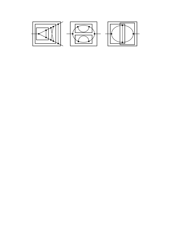
Beyond one-loop order, the process of the renormalization of a 1PI graph is characterized essentially by the appearance of its ultraviolet (UV) divergent 1PI Feynman subgraphs $\gamma_{i}\subset\Gamma$. For instance, two proper Feynman subgraphs $\gamma_{1},\ \gamma_{2}\subset\Gamma$ might be strictly nested, $\gamma_{1}\subset\gamma_{2}\subset\Gamma$, or disjoint, $\gamma_{1}\cap\gamma_{2}=\emptyset$. This hierarchy in which subgraphs are either located inside another subgraph or appear to be disjoint is best represented by a decorated rooted tree, see Section 3.5.3. However, there is a third possibility, consisting of subgraphs which might be overlapping, see Figure 1. In fact, such Feynman graphs are represented by linear combinations of decorated rooted trees. For a detailed treatment of this important case of overlapping graph structures in pQFT we refer to [Krei1999b].

Refer to caption
Figure 1: [Krei2000] There are various ways subdivergences can appear. They can be nested as in (a), disjoint as in (b) or overlapping as in (c). We put every subdivergence in a box. These boxes are called forests.

We denote by $F$ the set of all equivalence classes of one-particle irreducible Feynman graphs. Let ${\mathcal{F}}:=\mathbb{K}F$ be the $\mathbb{K}$-vector space with basis $F$. Let ${\mathcal{H}}_{\mathcal{F}}$ be the commutative polynomial algebra $\mathbb{K}[{\mathcal{F}}]$ with the product denoted by the disjoint union and with the empty graph $1_{\mathcal{F}}$ as the unit. Those 1PI Feynman graphs come with a grading by the number of loops. This gives rise to a grading on ${\mathcal{H}}_{\mathcal{F}}$ by $\deg(\prod_{i=1}^{k}\Gamma_{i})=\sum_{i=1}^{k}\deg(\Gamma_{i})$, making it into a connected graded commutative algebra ${{\mathcal{H}}}_{{\mathcal{F}}}=\oplus_{n=0}^{\infty}{\mathcal{H}}^{({n})}$ with ${\mathcal{H}}^{({n})}$ the subspace spanned by degree $n$ graphs. We have ${\mathcal{H}}^{({0})}\simeq\mathbb{K}$.

Define a counit $\epsilon$ on ${{\mathcal{H}}}_{{\mathcal{F}}}$ by $\epsilon(1_{\mathcal{F}})=1_{\mathbb{K}}$ and zero else. The key map is the coproduct $\Delta:{{\mathcal{H}}}_{{\mathcal{F}}}\to{{\mathcal{H}}}_{{\mathcal{F}}}\otimes{{\mathcal{H}}}_{{\mathcal{F}}}$ defined on 1PI Feynman graphs $\Gamma\in F$ by

$$\Delta(\Gamma)=\Gamma\otimes 1_{\mathcal{F}}+1_{\mathcal{F}}\otimes\Gamma+\sum_{\gamma{\subset}\Gamma}\gamma\otimes\Gamma/\gamma,$$ (95)

where by abuse of notation the sum is over all unions of disjoint divergent proper 1PI subgraphs $\gamma:=\{\gamma_{1}\cdots\gamma_{n}\}$, $\gamma_{i}\cap\gamma_{j}=\emptyset$, $i\neq j$, of $\Gamma$, and $\Gamma/\gamma$ denotes the cograph which follows from the contraction of $\gamma$ in $\Gamma$.

Remark 3.5

In fact, one may define the coproduct of a graph $\Gamma$ directly by the use of its spinneys in the wood $\bar{\mathfrak{W}}(\Gamma)$

$$\Delta(\Gamma)=\sum_{\{\gamma^{\prime}\}\in\bar{\mathfrak{W}}(\Gamma)}\gamma^{\prime}\otimes\Gamma/\{\gamma^{\prime}\}.$$ (96)

Where the first two terms $\Gamma\otimes 1_{\mathcal{F}}$ and $1_{\mathcal{F}}\otimes\Gamma$ follow from the spinneys $\{\Gamma\}$ and $\{\emptyset\}=:1_{\mathcal{F}}$, respectively. Hence, the coproduct can be seen as a tensor list, systematically storing term by term the spinneys and associated cographs for each Feynman graph.

We extend this definition to products of graphs (forests) in ${\mathcal{H}}_{\mathcal{F}}$, $\Delta\big{(}\prod_{i=1}^{k}\Gamma_{i}\big{)}=\prod_{i=1}^{k}\Delta(\Gamma_{i})$, so that we get a connected graded commutative non-cocommutative bialgebra, hence a Hopf algebra of that type with antipode map $S$, as defined in Eq. (36) . This result was first established by Connes and Kreimer in [CK2000]. By the definition of the coproduct in (95) we may call ${\mathcal{H}}_{{\mathcal{F}}}$ a renormalization Hopf algebra of Feynman graphs, since for $\Gamma\in F$ the cograph $\Gamma/\gamma$ in (95) always lies in $F$, such that

$${\mathcal{F}}\xrightarrow{\Delta}{\mathcal{H}}_{{\mathcal{F}}}\otimes{\mathcal{F}}.$$ (97)

As an example we calculate the coproduct of the graph \SetWidth3.0 \SetColorBlack \Line(105,-60)(240,-135) \Line(375,-60)(450,-60) \Line(240,-135)(240,15) \Line(375,-60)(240,-135) \Line(105,-60)(240,15) \Line(30,-60)(105,-60) \Line(240,15)(375,-60) missing-subexpression\SetWidth3.0 \SetColorBlack \Line(105,-60)(240,-135) \Line(375,-60)(450,-60) \Line(240,-135)(240,15) \Line(375,-60)(240,-135) \Line(105,-60)(240,15) \Line(30,-60)(105,-60) \Line(240,15)(375,-60) \begin{array}[]{c}\\[-11.38092pt] \!\scalebox{0.6}{{\scalebox{0.13}{ \begin{picture}(420.0,150.0)(30.0,-135.0)\SetWidth{3.0} \SetColor{Black} \Line(105,-60)(240,-135) \Line(375,-60)(450,-60) \Line(240,-135)(240,15) \Line(375,-60)(240,-135) \Line(105,-60)(240,15) \Line(30,-60)(105,-60) \Line(240,15)(375,-60) \end{picture}}}}\!\!\end{array}, borrowed from $\phi^{3}_{6}$ theory, which is the same as the graph in case (c) in Figure 1. We hope that the way we draw this two-loop Feynman self-energy graph now helps to identify its two one-loop vertex subgraphs, \SetWidth3.0 \SetColorBlack \Line(105,-60)(255,-135) \Line(105,-60)(255,15) \Line(225,-115)(225,-4) \Line(60,-60)(105,-60) missing-subexpression\SetWidth3.0 \SetColorBlack \Line(105,-60)(255,-135) \Line(105,-60)(255,15) \Line(225,-115)(225,-4) \Line(60,-60)(105,-60) \begin{array}[]{c}\\[-11.38092pt] \!\scalebox{0.6}{{\scalebox{0.13}{ \begin{picture}(195.0,150.0)(60.0,-135.0)\SetWidth{3.0} \SetColor{Black} \Line(105,-60)(255,-135) \Line(105,-60)(255,15) \Line(225,-115)(225,-4) \Line(60,-60)(105,-60) \end{picture}}}}\!\!\end{array} and \SetWidth3.0 \SetColorBlack \Line(135,-135)(285,-60) \Line(135,15)(285,-60) \Line(330,-60)(285,-60) \Line(165,-115)(165,-1) missing-subexpression\SetWidth3.0 \SetColorBlack \Line(135,-135)(285,-60) \Line(135,15)(285,-60) \Line(330,-60)(285,-60) \Line(165,-115)(165,-1) \begin{array}[]{c}\\[-11.38092pt] \!\scalebox{0.6}{{\scalebox{0.13}{ \begin{picture}(195.0,150.0)(135.0,-135.0)\SetWidth{3.0} \SetColor{Black} \Line(135,-135)(285,-60) \Line(135,15)(285,-60) \Line(330,-60)(285,-60) \Line(165,-115)(165,-1) \end{picture}}}}\!\!\end{array}.

Δ(\SetWidth3.0 \SetColorBlack \Line(105,-60)(240,-135) \Line(375,-60)(450,-60) \Line(240,-135)(240,15) \Line(375,-60)(240,-135) \Line(105,-60)(240,15) \Line(30,-60)(105,-60) \Line(240,15)(375,-60) )Δ\SetWidth3.0 \SetColorBlack \Line(105,-60)(240,-135) \Line(375,-60)(450,-60) \Line(240,-135)(240,15) \Line(375,-60)(240,-135) \Line(105,-60)(240,15) \Line(30,-60)(105,-60) \Line(240,15)(375,-60) \displaystyle\Delta\left(\!\!\!\begin{array}[]{c}\scalebox{0.6}{{\scalebox{0.13}{ \begin{picture}(420.0,150.0)(30.0,-135.0)\SetWidth{3.0} \SetColor{Black} \Line(105,-60)(240,-135) \Line(375,-60)(450,-60) \Line(240,-135)(240,15) \Line(375,-60)(240,-135) \Line(105,-60)(240,15) \Line(30,-60)(105,-60) \Line(240,15)(375,-60) \end{picture}}}}\\ \end{array}\!\!\!\right)\!\!\! $\displaystyle=$ \SetWidth3.0 \SetColorBlack \Line(105,-60)(240,-135) \Line(375,-60)(450,-60) \Line(240,-135)(240,15) \Line(375,-60)(240,-135) \Line(105,-60)(240,15) \Line(30,-60)(105,-60) \Line(240,15)(375,-60) 1+1\SetWidth3.0 \SetColorBlack \Line(105,-60)(240,-135) \Line(375,-60)(450,-60) \Line(240,-135)(240,15) \Line(375,-60)(240,-135) \Line(105,-60)(240,15) \Line(30,-60)(105,-60) \Line(240,15)(375,-60) +\SetWidth3.0 \SetColorBlack \Line(105,-60)(255,-135) \Line(105,-60)(255,15) \Line(225,-115)(225,-4) \Line(60,-60)(105,-60) \SetWidth3.0 \SetColorBlack \GOval(150,-120)(45,75)(0)1.0 \Line(75,-120)(15,-120) \Line(285,-120)(225,-120) +\SetWidth3.0 \SetColorBlack \Line(135,-135)(285,-60) \Line(135,15)(285,-60) \Line(330,-60)(285,-60) \Line(165,-115)(165,-1) \SetWidth3.0 \SetColorBlack \GOval(150,-120)(45,75)(0)1.0 \Line(75,-120)(15,-120) \Line(285,-120)(225,-120) .tensor-product\SetWidth3.0 \SetColorBlack \Line(105,-60)(240,-135) \Line(375,-60)(450,-60) \Line(240,-135)(240,15) \Line(375,-60)(240,-135) \Line(105,-60)(240,15) \Line(30,-60)(105,-60) \Line(240,15)(375,-60) subscript1tensor-productsubscript1\SetWidth3.0 \SetColorBlack \Line(105,-60)(240,-135) \Line(375,-60)(450,-60) \Line(240,-135)(240,15) \Line(375,-60)(240,-135) \Line(105,-60)(240,15) \Line(30,-60)(105,-60) \Line(240,15)(375,-60) tensor-product\SetWidth3.0 \SetColorBlack \Line(105,-60)(255,-135) \Line(105,-60)(255,15) \Line(225,-115)(225,-4) \Line(60,-60)(105,-60) \SetWidth3.0 \SetColorBlack \GOval(150,-120)(45,75)(0)1.0 \Line(75,-120)(15,-120) \Line(285,-120)(225,-120) tensor-product\SetWidth3.0 \SetColorBlack \Line(135,-135)(285,-60) \Line(135,15)(285,-60) \Line(330,-60)(285,-60) \Line(165,-115)(165,-1) \SetWidth3.0 \SetColorBlack \GOval(150,-120)(45,75)(0)1.0 \Line(75,-120)(15,-120) \Line(285,-120)(225,-120) \displaystyle\!\!\!\!\begin{array}[]{c}\scalebox{0.6}{{\scalebox{0.13}{ \begin{picture}(420.0,150.0)(30.0,-135.0)\SetWidth{3.0} \SetColor{Black} \Line(105,-60)(240,-135) \Line(375,-60)(450,-60) \Line(240,-135)(240,15) \Line(375,-60)(240,-135) \Line(105,-60)(240,15) \Line(30,-60)(105,-60) \Line(240,15)(375,-60) \end{picture}}}}\\ \end{array}\!\!\otimes 1_{\mathcal{F}}+1_{\mathcal{F}}\otimes\!\!\begin{array}[]{c}\scalebox{0.6}{{\scalebox{0.13}{ \begin{picture}(420.0,150.0)(30.0,-135.0)\SetWidth{3.0} \SetColor{Black} \Line(105,-60)(240,-135) \Line(375,-60)(450,-60) \Line(240,-135)(240,15) \Line(375,-60)(240,-135) \Line(105,-60)(240,15) \Line(30,-60)(105,-60) \Line(240,15)(375,-60) \end{picture}}}}\\ \end{array}\!+\!\begin{array}[]{c}\scalebox{0.6}{{\scalebox{0.13}{ \begin{picture}(195.0,150.0)(60.0,-135.0)\SetWidth{3.0} \SetColor{Black} \Line(105,-60)(255,-135) \Line(105,-60)(255,15) \Line(225,-115)(225,-4) \Line(60,-60)(105,-60) \end{picture}}}}\\ \end{array}\!\!\otimes\!\!\begin{array}[]{c}\scalebox{0.6}{{\scalebox{0.13}{ \begin{picture}(270.0,90.0)(15.0,-165.0)\SetWidth{3.0} \SetColor{Black} \GOval(150,-120)(45,75)(0){1.0} \Line(75,-120)(15,-120) \Line(285,-120)(225,-120) \end{picture}}}}\\ \end{array}\!+\!\begin{array}[]{c}\scalebox{0.6}{{\scalebox{0.13}{ \begin{picture}(195.0,150.0)(135.0,-135.0)\SetWidth{3.0} \SetColor{Black} \Line(135,-135)(285,-60) \Line(135,15)(285,-60) \Line(330,-60)(285,-60) \Line(165,-115)(165,-1) \end{picture}}}}\\ \end{array}\!\!\otimes\!\!\begin{array}[]{c}\scalebox{0.6}{{\scalebox{0.13}{ \begin{picture}(270.0,90.0)(15.0,-165.0)\SetWidth{3.0} \SetColor{Black} \GOval(150,-120)(45,75)(0){1.0} \Line(75,-120)(15,-120) \Line(285,-120)(225,-120) \end{picture}}}}\\ \end{array}.

Compare this with the wood containing the spinneys, 𝔚¯(\SetWidth3.0 \SetColorBlack \Line(105,-60)(240,-135) \Line(375,-60)(450,-60) \Line(240,-135)(240,15) \Line(375,-60)(240,-135) \Line(105,-60)(240,15) \Line(30,-60)(105,-60) \Line(240,15)(375,-60) )¯𝔚missing-subexpression\SetWidth3.0 \SetColorBlack \Line(105,-60)(240,-135) \Line(375,-60)(450,-60) \Line(240,-135)(240,15) \Line(375,-60)(240,-135) \Line(105,-60)(240,15) \Line(30,-60)(105,-60) \Line(240,15)(375,-60) \bar{\mathfrak{W}}\big{(}\!\!\begin{array}[]{c}\\[-9.95863pt] \scalebox{0.6}{{\scalebox{0.13}{ \begin{picture}(420.0,150.0)(30.0,-135.0)\SetWidth{3.0} \SetColor{Black} \Line(105,-60)(240,-135) \Line(375,-60)(450,-60) \Line(240,-135)(240,15) \Line(375,-60)(240,-135) \Line(105,-60)(240,15) \Line(30,-60)(105,-60) \Line(240,15)(375,-60) \end{picture}}}}\end{array}\!\!\big{)}, which is just given by Eq.(6) enlarged by the empty graph $\{\emptyset\}$ and the graph itself {\SetWidth3.0 \SetColorBlack \Line(105,-60)(240,-135) \Line(375,-60)(450,-60) \Line(240,-135)(240,15) \Line(375,-60)(240,-135) \Line(105,-60)(240,15) \Line(30,-60)(105,-60) \Line(240,15)(375,-60) }missing-subexpression\SetWidth3.0 \SetColorBlack \Line(105,-60)(240,-135) \Line(375,-60)(450,-60) \Line(240,-135)(240,15) \Line(375,-60)(240,-135) \Line(105,-60)(240,15) \Line(30,-60)(105,-60) \Line(240,15)(375,-60) \{\!\!\begin{array}[]{c}\\[-9.95863pt] \scalebox{0.6}{{\scalebox{0.13}{ \begin{picture}(420.0,150.0)(30.0,-135.0)\SetWidth{3.0} \SetColor{Black} \Line(105,-60)(240,-135) \Line(375,-60)(450,-60) \Line(240,-135)(240,15) \Line(375,-60)(240,-135) \Line(105,-60)(240,15) \Line(30,-60)(105,-60) \Line(240,15)(375,-60) \end{picture}}}}\end{array}\!\}.

Using Eq. (37) the antipode of this graph is given by

S(\SetWidth3.0 \SetColorBlack \Line(105,-60)(240,-135) \Line(375,-60)(450,-60) \Line(240,-135)(240,15) \Line(375,-60)(240,-135) \Line(105,-60)(240,15) \Line(30,-60)(105,-60) \Line(240,15)(375,-60) )𝑆\SetWidth3.0 \SetColorBlack \Line(105,-60)(240,-135) \Line(375,-60)(450,-60) \Line(240,-135)(240,15) \Line(375,-60)(240,-135) \Line(105,-60)(240,15) \Line(30,-60)(105,-60) \Line(240,15)(375,-60) \displaystyle S\left(\!\!\!\begin{array}[]{c}\scalebox{0.6}{{\scalebox{0.13}{ \begin{picture}(420.0,150.0)(30.0,-135.0)\SetWidth{3.0} \SetColor{Black} \Line(105,-60)(240,-135) \Line(375,-60)(450,-60) \Line(240,-135)(240,15) \Line(375,-60)(240,-135) \Line(105,-60)(240,15) \Line(30,-60)(105,-60) \Line(240,15)(375,-60) \end{picture}}}}\\ \end{array}\!\!\!\right)\!\!\! $\displaystyle=$ \SetWidth3.0 \SetColorBlack \Line(105,-60)(240,-135) \Line(375,-60)(450,-60) \Line(240,-135)(240,15) \Line(375,-60)(240,-135) \Line(105,-60)(240,15) \Line(30,-60)(105,-60) \Line(240,15)(375,-60) S(\SetWidth3.0 \SetColorBlack \Line(105,-60)(255,-135) \Line(105,-60)(255,15) \Line(225,-115)(225,-4) \Line(60,-60)(105,-60) )\SetWidth3.0 \SetColorBlack \GOval(150,-120)(45,75)(0)1.0 \Line(75,-120)(15,-120) \Line(285,-120)(225,-120) S(\SetWidth3.0 \SetColorBlack \Line(135,-135)(285,-60) \Line(135,15)(285,-60) \Line(330,-60)(285,-60) \Line(165,-115)(165,-1) )\SetWidth3.0 \SetColorBlack \GOval(150,-120)(45,75)(0)1.0 \Line(75,-120)(15,-120) \Line(285,-120)(225,-120)\SetWidth3.0 \SetColorBlack \Line(105,-60)(240,-135) \Line(375,-60)(450,-60) \Line(240,-135)(240,15) \Line(375,-60)(240,-135) \Line(105,-60)(240,15) \Line(30,-60)(105,-60) \Line(240,15)(375,-60) 𝑆\SetWidth3.0 \SetColorBlack \Line(105,-60)(255,-135) \Line(105,-60)(255,15) \Line(225,-115)(225,-4) \Line(60,-60)(105,-60) \SetWidth3.0 \SetColorBlack \GOval(150,-120)(45,75)(0)1.0 \Line(75,-120)(15,-120) \Line(285,-120)(225,-120) 𝑆\SetWidth3.0 \SetColorBlack \Line(135,-135)(285,-60) \Line(135,15)(285,-60) \Line(330,-60)(285,-60) \Line(165,-115)(165,-1) \SetWidth3.0 \SetColorBlack \GOval(150,-120)(45,75)(0)1.0 \Line(75,-120)(15,-120) \Line(285,-120)(225,-120)\displaystyle\!\!\!\!-\begin{array}[]{c}\scalebox{0.6}{{\scalebox{0.13}{ \begin{picture}(420.0,150.0)(30.0,-135.0)\SetWidth{3.0} \SetColor{Black} \Line(105,-60)(240,-135) \Line(375,-60)(450,-60) \Line(240,-135)(240,15) \Line(375,-60)(240,-135) \Line(105,-60)(240,15) \Line(30,-60)(105,-60) \Line(240,15)(375,-60) \end{picture}}}}\\ \end{array}-S\left(\!\!\!\begin{array}[]{c}\scalebox{0.6}{{\scalebox{0.13}{ \begin{picture}(195.0,150.0)(60.0,-135.0)\SetWidth{3.0} \SetColor{Black} \Line(105,-60)(255,-135) \Line(105,-60)(255,15) \Line(225,-115)(225,-4) \Line(60,-60)(105,-60) \end{picture}}}}\\ \end{array}\!\!\right)\!\!\begin{array}[]{c}\scalebox{0.6}{{\scalebox{0.13}{ \begin{picture}(270.0,90.0)(15.0,-165.0)\SetWidth{3.0} \SetColor{Black} \GOval(150,-120)(45,75)(0){1.0} \Line(75,-120)(15,-120) \Line(285,-120)(225,-120) \end{picture}}}}\\ \end{array}-S\left(\!\!\begin{array}[]{c}\scalebox{0.6}{{\scalebox{0.13}{ \begin{picture}(195.0,150.0)(135.0,-135.0)\SetWidth{3.0} \SetColor{Black} \Line(135,-135)(285,-60) \Line(135,15)(285,-60) \Line(330,-60)(285,-60) \Line(165,-115)(165,-1) \end{picture}}}}\\ \end{array}\!\!\right)\!\!\begin{array}[]{c}\scalebox{0.6}{{\scalebox{0.13}{ \begin{picture}(270.0,90.0)(15.0,-165.0)\SetWidth{3.0} \SetColor{Black} \GOval(150,-120)(45,75)(0){1.0} \Line(75,-120)(15,-120) \Line(285,-120)(225,-120) \end{picture}}}}\\ \end{array}

We must compare this with Bogoliubov’s classical formula for the counterterm $C(\Gamma)$ of a Feynman graph $\Gamma$, see Eq. (15) of Section 2.

C(\SetWidth3.0 \SetColorBlack \Line(105,-60)(240,-135) \Line(375,-60)(450,-60) \Line(240,-135)(240,15) \Line(375,-60)(240,-135) \Line(105,-60)(240,15) \Line(30,-60)(105,-60) \Line(240,15)(375,-60) )𝐶\SetWidth3.0 \SetColorBlack \Line(105,-60)(240,-135) \Line(375,-60)(450,-60) \Line(240,-135)(240,15) \Line(375,-60)(240,-135) \Line(105,-60)(240,15) \Line(30,-60)(105,-60) \Line(240,15)(375,-60) \displaystyle C\left(\!\!\!\begin{array}[]{c}\scalebox{0.6}{{\scalebox{0.13}{ \begin{picture}(420.0,150.0)(30.0,-135.0)\SetWidth{3.0} \SetColor{Black} \Line(105,-60)(240,-135) \Line(375,-60)(450,-60) \Line(240,-135)(240,15) \Line(375,-60)(240,-135) \Line(105,-60)(240,15) \Line(30,-60)(105,-60) \Line(240,15)(375,-60) \end{picture}}}}\\ \end{array}\!\!\!\right)\!\!\! $\displaystyle=$ R(\SetWidth3.0 \SetColorBlack \Line(105,-60)(240,-135) \Line(375,-60)(450,-60) \Line(240,-135)(240,15) \Line(375,-60)(240,-135) \Line(105,-60)(240,15) \Line(30,-60)(105,-60) \Line(240,15)(375,-60) +C(\SetWidth3.0 \SetColorBlack \Line(105,-60)(255,-135) \Line(105,-60)(255,15) \Line(225,-115)(225,-4) \Line(60,-60)(105,-60) )\SetWidth3.0 \SetColorBlack \GOval(150,-120)(45,75)(0)1.0 \Line(75,-120)(15,-120) \Line(285,-120)(225,-120) +C(\SetWidth3.0 \SetColorBlack \Line(135,-135)(285,-60) \Line(135,15)(285,-60) \Line(330,-60)(285,-60) \Line(165,-115)(165,-1) )\SetWidth3.0 \SetColorBlack \GOval(150,-120)(45,75)(0)1.0 \Line(75,-120)(15,-120) \Line(285,-120)(225,-120) )𝑅\SetWidth3.0 \SetColorBlack \Line(105,-60)(240,-135) \Line(375,-60)(450,-60) \Line(240,-135)(240,15) \Line(375,-60)(240,-135) \Line(105,-60)(240,15) \Line(30,-60)(105,-60) \Line(240,15)(375,-60) 𝐶\SetWidth3.0 \SetColorBlack \Line(105,-60)(255,-135) \Line(105,-60)(255,15) \Line(225,-115)(225,-4) \Line(60,-60)(105,-60) \SetWidth3.0 \SetColorBlack \GOval(150,-120)(45,75)(0)1.0 \Line(75,-120)(15,-120) \Line(285,-120)(225,-120) 𝐶\SetWidth3.0 \SetColorBlack \Line(135,-135)(285,-60) \Line(135,15)(285,-60) \Line(330,-60)(285,-60) \Line(165,-115)(165,-1) \SetWidth3.0 \SetColorBlack \GOval(150,-120)(45,75)(0)1.0 \Line(75,-120)(15,-120) \Line(285,-120)(225,-120) \displaystyle\!\!\!\!-R\left(\!\!\!\begin{array}[]{c}\scalebox{0.6}{{\scalebox{0.13}{ \begin{picture}(420.0,150.0)(30.0,-135.0)\SetWidth{3.0} \SetColor{Black} \Line(105,-60)(240,-135) \Line(375,-60)(450,-60) \Line(240,-135)(240,15) \Line(375,-60)(240,-135) \Line(105,-60)(240,15) \Line(30,-60)(105,-60) \Line(240,15)(375,-60) \end{picture}}}}\\ \end{array}+C\left(\!\!\!\begin{array}[]{c}\scalebox{0.6}{{\scalebox{0.13}{ \begin{picture}(195.0,150.0)(60.0,-135.0)\SetWidth{3.0} \SetColor{Black} \Line(105,-60)(255,-135) \Line(105,-60)(255,15) \Line(225,-115)(225,-4) \Line(60,-60)(105,-60) \end{picture}}}}\\ \end{array}\!\!\right)\!\!\begin{array}[]{c}\scalebox{0.8}{{\scalebox{0.13}{ \begin{picture}(270.0,90.0)(15.0,-165.0)\SetWidth{3.0} \SetColor{Black} \GOval(150,-120)(45,75)(0){1.0} \Line(75,-120)(15,-120) \Line(285,-120)(225,-120) \end{picture}}}}\\ \end{array}+C\left(\!\!\begin{array}[]{c}\scalebox{0.6}{{\scalebox{0.13}{ \begin{picture}(195.0,150.0)(135.0,-135.0)\SetWidth{3.0} \SetColor{Black} \Line(135,-135)(285,-60) \Line(135,15)(285,-60) \Line(330,-60)(285,-60) \Line(165,-115)(165,-1) \end{picture}}}}\\ \end{array}\!\!\right)\!\!\begin{array}[]{c}\scalebox{0.6}{{\scalebox{0.13}{ \begin{picture}(270.0,90.0)(15.0,-165.0)\SetWidth{3.0} \SetColor{Black} \GOval(150,-120)(45,75)(0){1.0} \Line(75,-120)(15,-120) \Line(285,-120)(225,-120) \end{picture}}}}\\ \end{array}\!\!\right)

Here, of course, each graph represents its corresponding –regularized– Feynman amplitude, and $R$ denotes the renormalization scheme map.

3.5.2 Lie and pre-Lie algebra of Feynman graphs

The combinatorial Hopf algebra of Feynman graphs has a dual counter part. To see this let us go back to the coproduct and antipode respectively the counterterm expression in the above example. In fact, we readily observe that the Connes-Kreimer coproduct just disentangles a graph analogously to Bogoliubov’s $\bar{\mathrm{R}}$-map which in turn gives the counterterm map $C$.

One might therefore think about an opposite operation in terms of gluing graphs into another graph. Let us define such a bilinear gluing operation on the vector space ${\mathcal{F}}$ of 1PI Feynman graphs

$$\Gamma_{1}*\Gamma_{2}=\sum_{\Gamma\in F}n(\Gamma_{1},\Gamma_{2};\Gamma)\Gamma.$$ (101)

The sum on the right hand side runs over all 1PI graphs $\Gamma$ in $F$. The number $n(\Gamma_{1},\Gamma_{2};\Gamma)\in\mathbb{N}$ for $\Gamma,\Gamma_{1},\Gamma_{2}\in F$ is a section coefficient which counts the number of ways a subgraph $\Gamma_{2}$ in $\Gamma$ can be reduced to a point such that $\Gamma_{1}$ is obtained. The above sum is finite as long as $\Gamma_{1}$ and $\Gamma_{2}$ are finite graphs. The graphs which contribute to this sum necessarily fulfill $\mathrm{deg}(\Gamma)=\mathrm{deg}(\Gamma_{1})+\mathrm{deg}(\Gamma_{2})$ and ${\bf res}(\Gamma)={\bf res}(\Gamma_{1})$, where we let ${\bf res}(\Gamma)$, called the residue of $\Gamma$, be the graph obtained when all internal edges are shrunk to a point. The graph we obtain in this manner consists of a single vertex with ${\bf res}(\Gamma)^{[0]}_{\mathrm{ext}}=\Gamma_{\mathrm{ext}}^{[0]}$. In case the initial graph was a self-energy graph, we regard its residue as a single edge.

As a matter of fact it was shown in several references [ChLi2001, CK1998, CK2002] that the operation $\ast$ on ${\mathcal{F}}$ defines a (right) pre-Lie product, satisfying the pre-Lie relation

$$(\Gamma_{1}\ast\Gamma_{2})\ast\Gamma_{3}-\Gamma_{1}\ast(\Gamma_{2}\ast\Gamma_{3})=(\Gamma_{1}\ast\Gamma_{3})\ast\Gamma_{2}-\Gamma_{1}\ast(\Gamma_{3}\ast\Gamma_{2})$$ (102)

and hence a pre-Lie algebra ${\mathcal{P}}:={\mathcal{P}}({\mathcal{F}})$. This pre-Lie algebra structure on Feynman graphs was further explored by Mencattini and Kreimer [MeKr2004, MeKr2005]. See also [EMK2003] for more details. The pre-Lie relation is sufficient for the anti-symmetrization of this product to fulfil the Jacobi identity. Hence, we get a graded Lie algebra ${{\mathcal{L}}}({\mathcal{P}}):=\bigoplus_{n\geq 0}{\mathcal{L}}^{({n})}$ of finite type, with commutator bracket

$$[\Gamma_{1},\ \Gamma_{2}]:=\Gamma_{1}\ast\Gamma_{2}-\Gamma_{2}\ast\Gamma_{1},$$ (103)

for $\Gamma_{1},\Gamma_{2}\in{\mathcal{F}}$. The above pre-Lie respectively Lie algebra structures are available once one has decided on the set of 1PI graphs $F$ of interest. The Milnor–Moore theorem [MM1965] then implies the structure of a corresponding Hopf algebra of Feynman graphs and vice versa.

So far we have two complementary operations on Feynman graphs forming either a (pre-)Lie or a Hopf algebra. In the former case we have a composition of Feynman graphs in terms of a pre-Lie gluing product, where we replace vertices by Feynman graphs with compatible external leg structure. Dually, we have the decomposition of graphs in terms of a Hopf algebra coproduct, i.e., replacing non-trivial UV divergent 1PI subgraphs by their residues.

3.5.3 Correspondence between non-planar rooted trees and Feynman graphs

Connes and Kreimer developed in [CK1998] a detailed picture of a connected graded commutative Hopf algebra structure of finite type on non-planar decorated rooted trees giving rise to an interesting interplay between perturbative renormalization and non-commutative geometry. This Hopf algebra of rooted trees serves as the role model for combinatorial Hopf algebras of the above type due to its universal property. In Section 3.4 we gave a brief account of its main properties. Here we would like to indicate its link to Feynman graphs and renormalization.

In the renormalization problem we associated to each graph $\Gamma$ its wood, i.e. the set of its spinneys, denoted by $\mathfrak{W}(\Gamma)$. We have seen that the coproduct is a storing list of those spinneys and the corresponding cographs. Indeed, the only information needed in this disentanglement problem of a graph is the hierarchical structure in which the spinneys appear to sit inside the graph. Each spinney of a graph consists of a union of disjoint UV divergent 1PI subgraphs $\gamma\subsetneq\Gamma$ which themselves may carry a nontrivial spinney structure, e.g. . Its set of proper spinneys was given in (7)

𝔚()={{},{}},𝔚\mathfrak{W}\Big{(}\parbox{18.0pt}{\begin{picture}(20.0,15.0)\put(6.4,0.0){\line(-1,3){6.4}} \put(6.4,0.0){\line(1,3){4.8}} \put(4.4,-1.5){\line(4,3){14.0}} \put(11.2,14.4){\line(2,-3){7.2}} \put(1.6,14.4){\qbezier(0.0,0.0)(4.8,4.8)(9.6,0.0)} \put(1.6,14.4){\qbezier(0.0,0.0)(4.8,-4.8)(9.6,0.0)} \end{picture}}\Big{)}=\big{\{}\{\parbox{18.0pt}{\begin{picture}(10.0,10.0)\put(1.0,5.0){\qbezier(0.0,-2.0)(8.0,10.0)(16.0,-2.0)} \put(1.0,5.0){\qbezier(0.0,2.0)(8.0,-10.0)(16.0,2.0)} \end{picture}}\},\{\parbox{16.79993pt}{\begin{picture}(10.0,10.0)\put(5.9,-1.4){\line(2,3){9.0}} \put(11.1,-1.4){\line(-2,3){9.0}} \put(4.0,7.5){\qbezier(0.0,1.8)(4.5,5.0)(9.0,1.8)} \put(4.0,7.5){\qbezier(0.0,1.8)(4.5,-1.25)(9.0,1.8)} \end{picture}}\}\big{\}},

where is a maximal spinney. We observe that this UV divergent 1PI subgraph  contains itself one –maximal– (sub)spinney

𝔚()={{}}.𝔚\mathfrak{W}(\parbox{16.79993pt}{\begin{picture}(10.0,10.0)\put(5.9,-1.4){\line(2,3){9.0}} \put(11.1,-1.4){\line(-2,3){9.0}} \put(4.0,7.5){\qbezier(0.0,1.8)(4.5,5.0)(9.0,1.8)} \put(4.0,7.5){\qbezier(0.0,1.8)(4.5,-1.25)(9.0,1.8)} \end{picture}})=\big{\{}\{\parbox{18.0pt}{\begin{picture}(10.0,10.0)\put(1.0,5.0){\qbezier(0.0,-2.0)(8.0,10.0)(16.0,-2.0)} \put(1.0,5.0){\qbezier(0.0,2.0)(8.0,-10.0)(16.0,2.0)} \end{picture}}\}\big{\}}.

For the graph
missing-subexpression
\begin{array}[]{c}\\[-11.38092pt] \scalebox{0.8}{\parbox{18.0pt}{\begin{picture}(10.0,10.0)\put(8.0,8.0){\circle{16.0}} \put(8.0,8.0){\qbezier(8.0,8.0)(0.0,0.0)(-8.0,8.0)} \put(8.0,8.0){\qbezier(8.0,-8.0)(0.0,0.0)(-8.0,-8.0)} \end{picture}}}\end{array}
we found

𝔚(
)
={{},{},{}}
.
𝔚missing-subexpression
\mathfrak{W}\Big{(}\!\!\begin{array}[]{c}\\[-14.22636pt] \scalebox{1.0}{\parbox{18.0pt}{\begin{picture}(10.0,10.0)\put(8.0,8.0){\circle{16.0}} \put(8.0,8.0){\qbezier(8.0,8.0)(0.0,0.0)(-8.0,8.0)} \put(8.0,8.0){\qbezier(8.0,-8.0)(0.0,0.0)(-8.0,-8.0)} \end{picture}}}\end{array}\!\!\Big{)}=\big{\{}\{\parbox{18.0pt}{\begin{picture}(10.0,10.0)\put(1.0,5.0){\qbezier(0.0,-2.0)(8.0,10.0)(16.0,-2.0)} \put(1.0,5.0){\qbezier(0.0,2.0)(8.0,-10.0)(16.0,2.0)} \end{picture}}\},\{\parbox{18.0pt}{\begin{picture}(10.0,10.0)\put(1.0,5.0){\qbezier(0.0,-2.0)(8.0,10.0)(16.0,-2.0)} \put(1.0,5.0){\qbezier(0.0,2.0)(8.0,-10.0)(16.0,2.0)} \end{picture}}\},\{\parbox{18.0pt}{\begin{picture}(10.0,10.0)\put(1.0,5.0){\qbezier(0.0,-2.0)(8.0,10.0)(16.0,-2.0)} \put(1.0,5.0){\qbezier(0.0,2.0)(8.0,-10.0)(16.0,2.0)} \end{picture}}\ \parbox{18.0pt}{\begin{picture}(10.0,10.0)\put(1.0,5.0){\qbezier(0.0,-2.0)(8.0,10.0)(16.0,-2.0)} \put(1.0,5.0){\qbezier(0.0,2.0)(8.0,-10.0)(16.0,2.0)} \end{picture}}\}\big{\}}.

Each of its 1PI subgraphs is primitive, and we have one maximal spinney which is the union {}\{\parbox{18.0pt}{\begin{picture}(10.0,10.0)\put(1.0,5.0){\qbezier(0.0,-2.0)(8.0,10.0)(16.0,-2.0)} \put(1.0,5.0){\qbezier(0.0,2.0)(8.0,-10.0)(16.0,2.0)} \end{picture}}\ \parbox{18.0pt}{\begin{picture}(10.0,10.0)\put(1.0,5.0){\qbezier(0.0,-2.0)(8.0,10.0)(16.0,-2.0)} \put(1.0,5.0){\qbezier(0.0,2.0)(8.0,-10.0)(16.0,2.0)} \end{picture}}\}. These hierarchies are best represented by rooted trees with vertices decorated by the primitive UV divergent 1PI $1$-loop graph

\SetWidth0.5 \SetColorBlack \Vertex(120,-9)5.66 \Vertex(120,-54)5.66 \Vertex(120,36)5.66 \SetWidth1.0 \Line(120,-9)(120,-54) \Line(120,36)(120,-24) \SetWidth0.9 \CArc(165,-31.5)(37.5,36.87,143.13) \CArc(165,28.5)(37.5,-143.13,-36.87) \CArc(165,73.5)(37.5,-143.13,-36.87) \CArc(165,13.5)(37.5,36.87,143.13) \CArc(165,-76.5)(37.5,36.87,143.13) \CArc(165,-16.5)(37.5,-143.13,-36.87)
\SetWidth0.5 \SetColorBlack \Vertex(120,-60)5.66 \Vertex(60,-60)5.66 \Vertex(90,-15)5.66 \SetWidth1.0 \Line(90,-15)(60,-60) \Line(90,-15)(120,-60) \SetWidth0.9 \CArc(45,-112.5)(37.5,36.87,143.13) \CArc(45,-52.5)(37.5,-143.13,-36.87) \CArc(135,-112.5)(37.5,36.87,143.13) \CArc(135,-52.5)(37.5,-143.13,-36.87) \CArc(105,37.5)(37.5,-143.13,-36.87) \CArc(105,-22.5)(37.5,36.87,143.13)
\SetWidth0.5 \SetColorBlack \Vertex(120,-9)5.66 \Vertex(120,-54)5.66 \Vertex(120,36)5.66 \SetWidth1.0 \Line(120,-9)(120,-54) \Line(120,36)(120,-24) \SetWidth0.9 \CArc(165,-31.5)(37.5,36.87,143.13) \CArc(165,28.5)(37.5,-143.13,-36.87) \CArc(165,73.5)(37.5,-143.13,-36.87) \CArc(165,13.5)(37.5,36.87,143.13) \CArc(165,-76.5)(37.5,36.87,143.13) \CArc(165,-16.5)(37.5,-143.13,-36.87) missing-subexpressionmissing-subexpressionsimilar-toabsent
\SetWidth0.5 \SetColorBlack \Vertex(120,-60)5.66 \Vertex(60,-60)5.66 \Vertex(90,-15)5.66 \SetWidth1.0 \Line(90,-15)(60,-60) \Line(90,-15)(120,-60) \SetWidth0.9 \CArc(45,-112.5)(37.5,36.87,143.13) \CArc(45,-52.5)(37.5,-143.13,-36.87) \CArc(135,-112.5)(37.5,36.87,143.13) \CArc(135,-52.5)(37.5,-143.13,-36.87) \CArc(105,37.5)(37.5,-143.13,-36.87) \CArc(105,-22.5)(37.5,36.87,143.13) missing-subexpressionmissing-subexpressionsimilar-toabsent
\begin{array}[]{cc}\scalebox{0.6}{\scalebox{0.8}{ \begin{picture}(81.0,111.0)(113.0,-60.0)\SetWidth{0.5} \SetColor{Black} \Vertex(120,-9){5.66} \Vertex(120,-54){5.66} \Vertex(120,36){5.66} \SetWidth{1.0} \Line(120,-9)(120,-54) \Line(120,36)(120,-24) \SetWidth{0.9} \CArc(165,-31.5)(37.5,36.87,143.13) \CArc(165,28.5)(37.5,-143.13,-36.87) \CArc(165,73.5)(37.5,-143.13,-36.87) \CArc(165,13.5)(37.5,36.87,143.13) \CArc(165,-76.5)(37.5,36.87,143.13) \CArc(165,-16.5)(37.5,-143.13,-36.87) \end{picture}}}&\\[-51.21504pt] &\sim\scalebox{2.0}{\parbox{18.0pt}{\begin{picture}(20.0,15.0)\put(6.4,0.0){\line(-1,3){6.4}} \put(6.4,0.0){\line(1,3){4.8}} \put(4.4,-1.5){\line(4,3){14.0}} \put(11.2,14.4){\line(2,-3){7.2}} \put(1.6,14.4){\qbezier(0.0,0.0)(4.8,4.8)(9.6,0.0)} \put(1.6,14.4){\qbezier(0.0,0.0)(4.8,-4.8)(9.6,0.0)} \end{picture}}}\\ \end{array}\;\;\qquad\;\;\begin{array}[]{cc}\scalebox{0.6}{\scalebox{0.8}{ \begin{picture}(150.0,105.0)(15.0,-90.0)\SetWidth{0.5} \SetColor{Black} \Vertex(120,-60){5.66} \Vertex(60,-60){5.66} \Vertex(90,-15){5.66} \SetWidth{1.0} \Line(90,-15)(60,-60) \Line(90,-15)(120,-60) \SetWidth{0.9} \CArc(45,-112.5)(37.5,36.87,143.13) \CArc(45,-52.5)(37.5,-143.13,-36.87) \CArc(135,-112.5)(37.5,36.87,143.13) \CArc(135,-52.5)(37.5,-143.13,-36.87) \CArc(105,37.5)(37.5,-143.13,-36.87) \CArc(105,-22.5)(37.5,36.87,143.13) \end{picture}}}&\\[-39.83368pt] &\sim\scalebox{1.5}{\parbox{18.0pt}{\begin{picture}(10.0,10.0)\put(8.0,8.0){\circle{16.0}} \put(8.0,8.0){\qbezier(8.0,8.0)(0.0,0.0)(-8.0,8.0)} \put(8.0,8.0){\qbezier(8.0,-8.0)(0.0,0.0)(-8.0,-8.0)} \end{picture}}}\\ \end{array}\\

The orientation of the graphs is of no importance at this level. The branching of the tree on the right hand side reflects the disjoint location of the subgraphs in
missing-subexpression
\begin{array}[]{c}\\[-11.38092pt] \scalebox{0.8}{\parbox{18.0pt}{\begin{picture}(10.0,10.0)\put(8.0,8.0){\circle{16.0}} \put(8.0,8.0){\qbezier(8.0,8.0)(0.0,0.0)(-8.0,8.0)} \put(8.0,8.0){\qbezier(8.0,-8.0)(0.0,0.0)(-8.0,-8.0)} \end{picture}}}\end{array}
, i.e. the spinney {}\{\parbox{18.0pt}{\begin{picture}(10.0,10.0)\put(1.0,5.0){\qbezier(0.0,-2.0)(8.0,10.0)(16.0,-2.0)} \put(1.0,5.0){\qbezier(0.0,2.0)(8.0,-10.0)(16.0,2.0)} \end{picture}}\ \parbox{18.0pt}{\begin{picture}(10.0,10.0)\put(1.0,5.0){\qbezier(0.0,-2.0)(8.0,10.0)(16.0,-2.0)} \put(1.0,5.0){\qbezier(0.0,2.0)(8.0,-10.0)(16.0,2.0)} \end{picture}}\}. Of course, different decorations may appear naturally in more complicated situations, like for instance in QED.

The property that both graphs have exactly one maximal spinney, that is, they contain no overlapping subgraphs, is reflected by the fact that their subdivergences hierarchy can be properly represented by a single decorated rooted tree. For graphs with overlapping subgraphs we have in general several maximal spinneys. For instance, recall the wood, i.e. the set of proper spinneys corresponding to the $3$-loop QED graph \SetWidth0.8 \SetColorBlack \Photon(60,0)(150,0)7.54 \SetWidth1.0 \ArrowLine(225,-75)(150,0) \ArrowLine(285,75)(360,0) \ArrowLine(225,75)(285,75) \ArrowLine(285,-75)(225,-75) \ArrowLine(360,0)(285,-75) \ArrowLine(150,0)(225,75) \SetWidth0.8 \Photon(60,0)(150,0)7.54 \Photon(360,0)(450,0)7.54 \Photon(225,75)(225,-75)7.57 \Photon(285,75)(285,-75)7.57 missing-subexpression\SetWidth0.8 \SetColorBlack \Photon(60,0)(150,0)7.54 \SetWidth1.0 \ArrowLine(225,-75)(150,0) \ArrowLine(285,75)(360,0) \ArrowLine(225,75)(285,75) \ArrowLine(285,-75)(225,-75) \ArrowLine(360,0)(285,-75) \ArrowLine(150,0)(225,75) \SetWidth0.8 \Photon(60,0)(150,0)7.54 \Photon(360,0)(450,0)7.54 \Photon(225,75)(225,-75)7.57 \Photon(285,75)(285,-75)7.57 \begin{array}[]{c}\\[-11.38092pt] \scalebox{0.5}{{\scalebox{0.2}{ \begin{picture}(390.0,150.0)(60.0,-75.0)\SetWidth{0.8} \SetColor{Black} \Photon(60,0)(150,0){7.5}{4} \SetWidth{1.0} \ArrowLine(225,-75)(150,0) \ArrowLine(285,75)(360,0) \ArrowLine(225,75)(285,75) \ArrowLine(285,-75)(225,-75) \ArrowLine(360,0)(285,-75) \ArrowLine(150,0)(225,75) \SetWidth{0.8} \Photon(60,0)(150,0){7.5}{4} \Photon(360,0)(450,0){7.5}{4} \Photon(225,75)(225,-75){7.5}{7} \Photon(285,75)(285,-75){7.5}{7} \end{picture}}}}\end{array}

𝔚(\SetWidth0.8 \SetColorBlack \Photon(60,0)(150,0)7.54 \SetWidth1.0 \ArrowLine(225,-75)(150,0) \ArrowLine(285,75)(360,0) \ArrowLine(225,75)(285,75) \ArrowLine(285,-75)(225,-75) \ArrowLine(360,0)(285,-75) \ArrowLine(150,0)(225,75) \SetWidth0.8 \Photon(60,0)(150,0)7.54 \Photon(360,0)(450,0)7.54 \Photon(225,75)(225,-75)7.57 \Photon(285,75)(285,-75)7.57 )={{\SetWidth1.0 \SetColorBlack \ArrowLine(285,75)(360,0) \ArrowLine(360,0)(285,-75) \SetWidth0.8 \Photon(360,0)(450,0)7.54 \Photon(285,75)(285,-75)7.57 \SetWidth1.0 \ArrowLine(285,-75)(255,-75) \ArrowLine(255,75)(285,75) },{\SetWidth0.8 \SetColorBlack \Photon(60,0)(150,0)7.54 \SetWidth1.0 \ArrowLine(225,-75)(150,0) \ArrowLine(150,0)(225,75) \SetWidth0.8 \Photon(60,0)(150,0)7.54 \Photon(225,75)(225,-75)7.57 \SetWidth1.0 \ArrowLine(255,-75)(225,-75) \ArrowLine(225,75)(255,75) },{\SetWidth0.8 \SetColorBlack \Photon(60,0)(150,0)7.54 \SetWidth1.0 \ArrowLine(225,-75)(150,0) \ArrowLine(225,75)(285,75) \ArrowLine(285,-75)(225,-75) \ArrowLine(150,0)(225,75) \SetWidth0.8 \Photon(60,0)(150,0)7.54 \Photon(225,75)(225,-75)7.57 \Photon(285,75)(285,-75)7.57 \SetWidth1.0 \ArrowLine(315,-75)(285,-75) \ArrowLine(285,75)(315,75) },{\SetWidth1.0 \SetColorBlack \ArrowLine(285,75)(360,0) \ArrowLine(225,75)(285,75) \ArrowLine(285,-75)(225,-75) \ArrowLine(360,0)(285,-75) \SetWidth0.8 \Photon(360,0)(450,0)7.54 \Photon(225,75)(225,-75)7.57 \Photon(285,75)(285,-75)7.57 \SetWidth1.0 \ArrowLine(225,-75)(180,-75) \ArrowLine(180,75)(225,75) },{\SetWidth0.8 \SetColorBlack \Photon(60,0)(150,0)7.54 \SetWidth1.0 \ArrowLine(225,-75)(150,0) \ArrowLine(150,0)(225,75) \SetWidth0.8 \Photon(60,0)(150,0)7.54 \Photon(225,75)(225,-75)7.57 \SetWidth1.0 \ArrowLine(255,-75)(225,-75) \ArrowLine(225,75)(255,75) \SetWidth1.0 \SetColorBlack \ArrowLine(285,75)(360,0) \ArrowLine(360,0)(285,-75) \SetWidth0.8 \Photon(360,0)(450,0)7.54 \Photon(285,75)(285,-75)7.57 \SetWidth1.0 \ArrowLine(285,-75)(255,-75) \ArrowLine(255,75)(285,75) }}𝔚missing-subexpression\SetWidth0.8 \SetColorBlack \Photon(60,0)(150,0)7.54 \SetWidth1.0 \ArrowLine(225,-75)(150,0) \ArrowLine(285,75)(360,0) \ArrowLine(225,75)(285,75) \ArrowLine(285,-75)(225,-75) \ArrowLine(360,0)(285,-75) \ArrowLine(150,0)(225,75) \SetWidth0.8 \Photon(60,0)(150,0)7.54 \Photon(360,0)(450,0)7.54 \Photon(225,75)(225,-75)7.57 \Photon(285,75)(285,-75)7.57 missing-subexpression\SetWidth1.0 \SetColorBlack \ArrowLine(285,75)(360,0) \ArrowLine(360,0)(285,-75) \SetWidth0.8 \Photon(360,0)(450,0)7.54 \Photon(285,75)(285,-75)7.57 \SetWidth1.0 \ArrowLine(285,-75)(255,-75) \ArrowLine(255,75)(285,75) missing-subexpression\SetWidth0.8 \SetColorBlack \Photon(60,0)(150,0)7.54 \SetWidth1.0 \ArrowLine(225,-75)(150,0) \ArrowLine(150,0)(225,75) \SetWidth0.8 \Photon(60,0)(150,0)7.54 \Photon(225,75)(225,-75)7.57 \SetWidth1.0 \ArrowLine(255,-75)(225,-75) \ArrowLine(225,75)(255,75) missing-subexpression\SetWidth0.8 \SetColorBlack \Photon(60,0)(150,0)7.54 \SetWidth1.0 \ArrowLine(225,-75)(150,0) \ArrowLine(225,75)(285,75) \ArrowLine(285,-75)(225,-75) \ArrowLine(150,0)(225,75) \SetWidth0.8 \Photon(60,0)(150,0)7.54 \Photon(225,75)(225,-75)7.57 \Photon(285,75)(285,-75)7.57 \SetWidth1.0 \ArrowLine(315,-75)(285,-75) \ArrowLine(285,75)(315,75) missing-subexpression\SetWidth1.0 \SetColorBlack \ArrowLine(285,75)(360,0) \ArrowLine(225,75)(285,75) \ArrowLine(285,-75)(225,-75) \ArrowLine(360,0)(285,-75) \SetWidth0.8 \Photon(360,0)(450,0)7.54 \Photon(225,75)(225,-75)7.57 \Photon(285,75)(285,-75)7.57 \SetWidth1.0 \ArrowLine(225,-75)(180,-75) \ArrowLine(180,75)(225,75) casesmissing-subexpression\SetWidth0.8 \SetColorBlack \Photon(60,0)(150,0)7.54 \SetWidth1.0 \ArrowLine(225,-75)(150,0) \ArrowLine(150,0)(225,75) \SetWidth0.8 \Photon(60,0)(150,0)7.54 \Photon(225,75)(225,-75)7.57 \SetWidth1.0 \ArrowLine(255,-75)(225,-75) \ArrowLine(225,75)(255,75) casesmissing-subexpression\SetWidth1.0 \SetColorBlack \ArrowLine(285,75)(360,0) \ArrowLine(360,0)(285,-75) \SetWidth0.8 \Photon(360,0)(450,0)7.54 \Photon(285,75)(285,-75)7.57 \SetWidth1.0 \ArrowLine(285,-75)(255,-75) \ArrowLine(255,75)(285,75) \mathfrak{W}\left(\!\!\!\!\begin{array}[]{c}\\[-11.38092pt] \scalebox{0.55}{{\scalebox{0.2}{ \begin{picture}(390.0,150.0)(60.0,-75.0)\SetWidth{0.8} \SetColor{Black} \Photon(60,0)(150,0){7.5}{4} \SetWidth{1.0} \ArrowLine(225,-75)(150,0) \ArrowLine(285,75)(360,0) \ArrowLine(225,75)(285,75) \ArrowLine(285,-75)(225,-75) \ArrowLine(360,0)(285,-75) \ArrowLine(150,0)(225,75) \SetWidth{0.8} \Photon(60,0)(150,0){7.5}{4} \Photon(360,0)(450,0){7.5}{4} \Photon(225,75)(225,-75){7.5}{7} \Photon(285,75)(285,-75){7.5}{7} \end{picture}}}}\end{array}\!\!\!\!\right)=\left\{\Big{\{}\!\!\begin{array}[]{c}\\[-11.38092pt] \scalebox{0.55}{{\scalebox{0.2}{ \begin{picture}(195.0,150.0)(255.0,-75.0)\SetWidth{1.0} \SetColor{Black} \ArrowLine(285,75)(360,0) \ArrowLine(360,0)(285,-75) \SetWidth{0.8} \Photon(360,0)(450,0){7.5}{4} \Photon(285,75)(285,-75){7.5}{7} \SetWidth{1.0} \ArrowLine(285,-75)(255,-75) \ArrowLine(255,75)(285,75) \end{picture}}}}\end{array}\!\!\Big{\}},\Big{\{}\!\!\begin{array}[]{c}\\[-11.38092pt] \scalebox{0.55}{{\scalebox{0.2}{ \begin{picture}(195.0,150.0)(60.0,-75.0)\SetWidth{0.8} \SetColor{Black} \Photon(60,0)(150,0){7.5}{4} \SetWidth{1.0} \ArrowLine(225,-75)(150,0) \ArrowLine(150,0)(225,75) \SetWidth{0.8} \Photon(60,0)(150,0){7.5}{4} \Photon(225,75)(225,-75){7.5}{7} \SetWidth{1.0} \ArrowLine(255,-75)(225,-75) \ArrowLine(225,75)(255,75) \end{picture}}}}\end{array}\!\!\Big{\}},\Big{\{}\!\!\begin{array}[]{c}\\[-11.38092pt] \scalebox{0.55}{{\scalebox{0.2}{ \begin{picture}(255.0,150.0)(60.0,-75.0)\SetWidth{0.8} \SetColor{Black} \Photon(60,0)(150,0){7.5}{4} \SetWidth{1.0} \ArrowLine(225,-75)(150,0) \ArrowLine(225,75)(285,75) \ArrowLine(285,-75)(225,-75) \ArrowLine(150,0)(225,75) \SetWidth{0.8} \Photon(60,0)(150,0){7.5}{4} \Photon(225,75)(225,-75){7.5}{7} \Photon(285,75)(285,-75){7.5}{7} \SetWidth{1.0} \ArrowLine(315,-75)(285,-75) \ArrowLine(285,75)(315,75) \end{picture}}}}\end{array}\!\!\Big{\}},\Big{\{}\!\!\begin{array}[]{c}\\[-11.38092pt] \scalebox{0.55}{{\scalebox{0.2}{ \begin{picture}(270.0,150.0)(180.0,-75.0)\SetWidth{1.0} \SetColor{Black} \ArrowLine(285,75)(360,0) \ArrowLine(225,75)(285,75) \ArrowLine(285,-75)(225,-75) \ArrowLine(360,0)(285,-75) \SetWidth{0.8} \Photon(360,0)(450,0){7.5}{4} \Photon(225,75)(225,-75){7.5}{7} \Photon(285,75)(285,-75){7.5}{7} \SetWidth{1.0} \ArrowLine(225,-75)(180,-75) \ArrowLine(180,75)(225,75) \end{picture}}}}\end{array}\!\!\Big{\}},\Big{\{}\!\!\begin{array}[]{c}\\[-11.38092pt] \scalebox{0.55}{{\scalebox{0.2}{ \begin{picture}(195.0,150.0)(60.0,-75.0)\SetWidth{0.8} \SetColor{Black} \Photon(60,0)(150,0){7.5}{4} \SetWidth{1.0} \ArrowLine(225,-75)(150,0) \ArrowLine(150,0)(225,75) \SetWidth{0.8} \Photon(60,0)(150,0){7.5}{4} \Photon(225,75)(225,-75){7.5}{7} \SetWidth{1.0} \ArrowLine(255,-75)(225,-75) \ArrowLine(225,75)(255,75) \end{picture}}}}\end{array}\!\begin{array}[]{c}\\[-11.38092pt] \scalebox{0.55}{{\scalebox{0.2}{ \begin{picture}(195.0,150.0)(255.0,-75.0)\SetWidth{1.0} \SetColor{Black} \ArrowLine(285,75)(360,0) \ArrowLine(360,0)(285,-75) \SetWidth{0.8} \Photon(360,0)(450,0){7.5}{4} \Photon(285,75)(285,-75){7.5}{7} \SetWidth{1.0} \ArrowLine(285,-75)(255,-75) \ArrowLine(255,75)(285,75) \end{picture}}}}\end{array}\!\!\Big{\}}\right\}

with the following cographs

\SetWidth0.8 \SetColorBlack \Photon(60,0)(150,0)7.54 \SetWidth1.0 \ArrowLine(225,-75)(150,0) \ArrowLine(285,75)(360,0) \ArrowLine(225,75)(285,75) \ArrowLine(285,-75)(225,-75) \ArrowLine(360,0)(285,-75) \ArrowLine(150,0)(225,75) \SetWidth0.8 \Photon(60,0)(150,0)7.54 \Photon(360,0)(450,0)7.54 \Photon(225,75)(225,-75)7.57 \Photon(285,75)(285,-75)7.57 /{\SetWidth1.0 \SetColorBlack \ArrowLine(285,75)(360,0) \ArrowLine(360,0)(285,-75) \SetWidth0.8 \Photon(360,0)(450,0)7.54 \Photon(285,75)(285,-75)7.57 \SetWidth1.0 \ArrowLine(285,-75)(255,-75) \ArrowLine(255,75)(285,75) }=\SetWidth0.8 \SetColorBlack \Photon(60,0)(150,0)7.54 \SetWidth1.0 \ArrowLine(225,-75)(150,0) \ArrowLine(150,0)(225,75) \SetWidth0.8 \Photon(60,0)(150,0)7.54 \Photon(225,75)(225,-75)7.57 \SetWidth1.0 \ArrowLine(225,75)(300,0) \ArrowLine(300,0)(225,-75) \SetWidth0.8 \Photon(300,0)(390,0)7.54 =\SetWidth0.8 \SetColorBlack \Photon(60,0)(150,0)7.54 \SetWidth1.0 \ArrowLine(225,-75)(150,0) \ArrowLine(285,75)(360,0) \ArrowLine(225,75)(285,75) \ArrowLine(285,-75)(225,-75) \ArrowLine(360,0)(285,-75) \ArrowLine(150,0)(225,75) \SetWidth0.8 \Photon(60,0)(150,0)7.54 \Photon(360,0)(450,0)7.54 \Photon(225,75)(225,-75)7.57 \Photon(285,75)(285,-75)7.57 /{\SetWidth0.8 \SetColorBlack \Photon(60,0)(150,0)7.54 \SetWidth1.0 \ArrowLine(225,-75)(150,0) \ArrowLine(150,0)(225,75) \SetWidth0.8 \Photon(60,0)(150,0)7.54 \Photon(225,75)(225,-75)7.57 \SetWidth1.0 \ArrowLine(255,-75)(225,-75) \ArrowLine(225,75)(255,75) }missing-subexpression\SetWidth0.8 \SetColorBlack \Photon(60,0)(150,0)7.54 \SetWidth1.0 \ArrowLine(225,-75)(150,0) \ArrowLine(285,75)(360,0) \ArrowLine(225,75)(285,75) \ArrowLine(285,-75)(225,-75) \ArrowLine(360,0)(285,-75) \ArrowLine(150,0)(225,75) \SetWidth0.8 \Photon(60,0)(150,0)7.54 \Photon(360,0)(450,0)7.54 \Photon(225,75)(225,-75)7.57 \Photon(285,75)(285,-75)7.57 missing-subexpression\SetWidth1.0 \SetColorBlack \ArrowLine(285,75)(360,0) \ArrowLine(360,0)(285,-75) \SetWidth0.8 \Photon(360,0)(450,0)7.54 \Photon(285,75)(285,-75)7.57 \SetWidth1.0 \ArrowLine(285,-75)(255,-75) \ArrowLine(255,75)(285,75) missing-subexpression\SetWidth0.8 \SetColorBlack \Photon(60,0)(150,0)7.54 \SetWidth1.0 \ArrowLine(225,-75)(150,0) \ArrowLine(150,0)(225,75) \SetWidth0.8 \Photon(60,0)(150,0)7.54 \Photon(225,75)(225,-75)7.57 \SetWidth1.0 \ArrowLine(225,75)(300,0) \ArrowLine(300,0)(225,-75) \SetWidth0.8 \Photon(300,0)(390,0)7.54 missing-subexpression\SetWidth0.8 \SetColorBlack \Photon(60,0)(150,0)7.54 \SetWidth1.0 \ArrowLine(225,-75)(150,0) \ArrowLine(285,75)(360,0) \ArrowLine(225,75)(285,75) \ArrowLine(285,-75)(225,-75) \ArrowLine(360,0)(285,-75) \ArrowLine(150,0)(225,75) \SetWidth0.8 \Photon(60,0)(150,0)7.54 \Photon(360,0)(450,0)7.54 \Photon(225,75)(225,-75)7.57 \Photon(285,75)(285,-75)7.57 missing-subexpression\SetWidth0.8 \SetColorBlack \Photon(60,0)(150,0)7.54 \SetWidth1.0 \ArrowLine(225,-75)(150,0) \ArrowLine(150,0)(225,75) \SetWidth0.8 \Photon(60,0)(150,0)7.54 \Photon(225,75)(225,-75)7.57 \SetWidth1.0 \ArrowLine(255,-75)(225,-75) \ArrowLine(225,75)(255,75) \begin{array}[]{c}\\[-8.5359pt] \scalebox{0.55}{{\scalebox{0.2}{ \begin{picture}(390.0,150.0)(60.0,-75.0)\SetWidth{0.8} \SetColor{Black} \Photon(60,0)(150,0){7.5}{4} \SetWidth{1.0} \ArrowLine(225,-75)(150,0) \ArrowLine(285,75)(360,0) \ArrowLine(225,75)(285,75) \ArrowLine(285,-75)(225,-75) \ArrowLine(360,0)(285,-75) \ArrowLine(150,0)(225,75) \SetWidth{0.8} \Photon(60,0)(150,0){7.5}{4} \Photon(360,0)(450,0){7.5}{4} \Photon(225,75)(225,-75){7.5}{7} \Photon(285,75)(285,-75){7.5}{7} \end{picture}}}}\end{array}\big{/}\Big{\{}\!\!\begin{array}[]{c}\\[-11.38092pt] \scalebox{0.55}{{\scalebox{0.2}{ \begin{picture}(195.0,150.0)(255.0,-75.0)\SetWidth{1.0} \SetColor{Black} \ArrowLine(285,75)(360,0) \ArrowLine(360,0)(285,-75) \SetWidth{0.8} \Photon(360,0)(450,0){7.5}{4} \Photon(285,75)(285,-75){7.5}{7} \SetWidth{1.0} \ArrowLine(285,-75)(255,-75) \ArrowLine(255,75)(285,75) \end{picture}}}}\end{array}\!\!\Big{\}}=\!\!\begin{array}[]{c}\\[-11.38092pt] \scalebox{0.55}{{\scalebox{0.2}{ \begin{picture}(330.0,150.0)(60.0,-75.0)\SetWidth{0.8} \SetColor{Black} \Photon(60,0)(150,0){7.5}{4} \SetWidth{1.0} \ArrowLine(225,-75)(150,0) \ArrowLine(150,0)(225,75) \SetWidth{0.8} \Photon(60,0)(150,0){7.5}{4} \Photon(225,75)(225,-75){7.5}{7} \SetWidth{1.0} \ArrowLine(225,75)(300,0) \ArrowLine(300,0)(225,-75) \SetWidth{0.8} \Photon(300,0)(390,0){7.5}{4} \end{picture}}}}\end{array}=\!\!\begin{array}[]{c}\\[-11.38092pt] \scalebox{0.55}{{\scalebox{0.2}{ \begin{picture}(390.0,150.0)(60.0,-75.0)\SetWidth{0.8} \SetColor{Black} \Photon(60,0)(150,0){7.5}{4} \SetWidth{1.0} \ArrowLine(225,-75)(150,0) \ArrowLine(285,75)(360,0) \ArrowLine(225,75)(285,75) \ArrowLine(285,-75)(225,-75) \ArrowLine(360,0)(285,-75) \ArrowLine(150,0)(225,75) \SetWidth{0.8} \Photon(60,0)(150,0){7.5}{4} \Photon(360,0)(450,0){7.5}{4} \Photon(225,75)(225,-75){7.5}{7} \Photon(285,75)(285,-75){7.5}{7} \end{picture}}}}\end{array}\big{/}\ \Big{\{}\!\!\begin{array}[]{c}\\[-11.38092pt] \scalebox{0.55}{{\scalebox{0.2}{ \begin{picture}(195.0,150.0)(60.0,-75.0)\SetWidth{0.8} \SetColor{Black} \Photon(60,0)(150,0){7.5}{4} \SetWidth{1.0} \ArrowLine(225,-75)(150,0) \ArrowLine(150,0)(225,75) \SetWidth{0.8} \Photon(60,0)(150,0){7.5}{4} \Photon(225,75)(225,-75){7.5}{7} \SetWidth{1.0} \ArrowLine(255,-75)(225,-75) \ArrowLine(225,75)(255,75) \end{picture}}}}\end{array}\!\!\Big{\}}

and

\SetWidth0.8 \SetColorBlack \Photon(60,0)(150,0)7.54 \SetWidth1.0 \ArrowLine(225,-75)(150,0) \ArrowLine(285,75)(360,0) \ArrowLine(225,75)(285,75) \ArrowLine(285,-75)(225,-75) \ArrowLine(360,0)(285,-75) \ArrowLine(150,0)(225,75) \SetWidth0.8 \Photon(60,0)(150,0)7.54 \Photon(360,0)(450,0)7.54 \Photon(225,75)(225,-75)7.57 \Photon(285,75)(285,-75)7.57 /{\SetWidth0.8 \SetColorBlack \Photon(60,0)(150,0)7.54 \SetWidth1.0 \ArrowLine(225,-75)(150,0) \ArrowLine(225,75)(285,75) \ArrowLine(285,-75)(225,-75) \ArrowLine(150,0)(225,75) \SetWidth0.8 \Photon(60,0)(150,0)7.54 \Photon(225,75)(225,-75)7.57 \Photon(285,75)(285,-75)7.57 \SetWidth1.0 \ArrowLine(315,-75)(285,-75) \ArrowLine(285,75)(315,75) }missing-subexpression\SetWidth0.8 \SetColorBlack \Photon(60,0)(150,0)7.54 \SetWidth1.0 \ArrowLine(225,-75)(150,0) \ArrowLine(285,75)(360,0) \ArrowLine(225,75)(285,75) \ArrowLine(285,-75)(225,-75) \ArrowLine(360,0)(285,-75) \ArrowLine(150,0)(225,75) \SetWidth0.8 \Photon(60,0)(150,0)7.54 \Photon(360,0)(450,0)7.54 \Photon(225,75)(225,-75)7.57 \Photon(285,75)(285,-75)7.57 missing-subexpression\SetWidth0.8 \SetColorBlack \Photon(60,0)(150,0)7.54 \SetWidth1.0 \ArrowLine(225,-75)(150,0) \ArrowLine(225,75)(285,75) \ArrowLine(285,-75)(225,-75) \ArrowLine(150,0)(225,75) \SetWidth0.8 \Photon(60,0)(150,0)7.54 \Photon(225,75)(225,-75)7.57 \Photon(285,75)(285,-75)7.57 \SetWidth1.0 \ArrowLine(315,-75)(285,-75) \ArrowLine(285,75)(315,75) \displaystyle\begin{array}[]{c}\\[-11.38092pt] \scalebox{0.55}{{\scalebox{0.2}{ \begin{picture}(390.0,150.0)(60.0,-75.0)\SetWidth{0.8} \SetColor{Black} \Photon(60,0)(150,0){7.5}{4} \SetWidth{1.0} \ArrowLine(225,-75)(150,0) \ArrowLine(285,75)(360,0) \ArrowLine(225,75)(285,75) \ArrowLine(285,-75)(225,-75) \ArrowLine(360,0)(285,-75) \ArrowLine(150,0)(225,75) \SetWidth{0.8} \Photon(60,0)(150,0){7.5}{4} \Photon(360,0)(450,0){7.5}{4} \Photon(225,75)(225,-75){7.5}{7} \Photon(285,75)(285,-75){7.5}{7} \end{picture}}}}\end{array}\big{/}\ \Big{\{}\!\!\begin{array}[]{c}\\[-11.38092pt] \scalebox{0.55}{{\scalebox{0.2}{ \begin{picture}(255.0,150.0)(60.0,-75.0)\SetWidth{0.8} \SetColor{Black} \Photon(60,0)(150,0){7.5}{4} \SetWidth{1.0} \ArrowLine(225,-75)(150,0) \ArrowLine(225,75)(285,75) \ArrowLine(285,-75)(225,-75) \ArrowLine(150,0)(225,75) \SetWidth{0.8} \Photon(60,0)(150,0){7.5}{4} \Photon(225,75)(225,-75){7.5}{7} \Photon(285,75)(285,-75){7.5}{7} \SetWidth{1.0} \ArrowLine(315,-75)(285,-75) \ArrowLine(285,75)(315,75) \end{picture}}}}\end{array}\!\!\Big{\}} $\displaystyle=$ \SetWidth0.8 \SetColorBlack \Photon(60,0)(150,0)7.54 \SetWidth1.0 \ArrowLine(225,-75)(150,0) \ArrowLine(285,75)(360,0) \ArrowLine(225,75)(285,75) \ArrowLine(285,-75)(225,-75) \ArrowLine(360,0)(285,-75) \ArrowLine(150,0)(225,75) \SetWidth0.8 \Photon(60,0)(150,0)7.54 \Photon(360,0)(450,0)7.54 \Photon(225,75)(225,-75)7.57 \Photon(285,75)(285,-75)7.57 /{\SetWidth1.0 \SetColorBlack \ArrowLine(285,75)(360,0) \ArrowLine(225,75)(285,75) \ArrowLine(285,-75)(225,-75) \ArrowLine(360,0)(285,-75) \SetWidth0.8 \Photon(360,0)(450,0)7.54 \Photon(225,75)(225,-75)7.57 \Photon(285,75)(285,-75)7.57 \SetWidth1.0 \ArrowLine(225,-75)(180,-75) \ArrowLine(180,75)(225,75) }missing-subexpression\SetWidth0.8 \SetColorBlack \Photon(60,0)(150,0)7.54 \SetWidth1.0 \ArrowLine(225,-75)(150,0) \ArrowLine(285,75)(360,0) \ArrowLine(225,75)(285,75) \ArrowLine(285,-75)(225,-75) \ArrowLine(360,0)(285,-75) \ArrowLine(150,0)(225,75) \SetWidth0.8 \Photon(60,0)(150,0)7.54 \Photon(360,0)(450,0)7.54 \Photon(225,75)(225,-75)7.57 \Photon(285,75)(285,-75)7.57 missing-subexpression\SetWidth1.0 \SetColorBlack \ArrowLine(285,75)(360,0) \ArrowLine(225,75)(285,75) \ArrowLine(285,-75)(225,-75) \ArrowLine(360,0)(285,-75) \SetWidth0.8 \Photon(360,0)(450,0)7.54 \Photon(225,75)(225,-75)7.57 \Photon(285,75)(285,-75)7.57 \SetWidth1.0 \ArrowLine(225,-75)(180,-75) \ArrowLine(180,75)(225,75) \displaystyle\begin{array}[]{c}\\[-11.38092pt] \scalebox{0.55}{{\scalebox{0.2}{ \begin{picture}(390.0,150.0)(60.0,-75.0)\SetWidth{0.8} \SetColor{Black} \Photon(60,0)(150,0){7.5}{4} \SetWidth{1.0} \ArrowLine(225,-75)(150,0) \ArrowLine(285,75)(360,0) \ArrowLine(225,75)(285,75) \ArrowLine(285,-75)(225,-75) \ArrowLine(360,0)(285,-75) \ArrowLine(150,0)(225,75) \SetWidth{0.8} \Photon(60,0)(150,0){7.5}{4} \Photon(360,0)(450,0){7.5}{4} \Photon(225,75)(225,-75){7.5}{7} \Photon(285,75)(285,-75){7.5}{7} \end{picture}}}}\end{array}\big{/}\ \Big{\{}\!\!\begin{array}[]{c}\\[-11.38092pt] \scalebox{0.55}{{\scalebox{0.2}{ \begin{picture}(270.0,150.0)(180.0,-75.0)\SetWidth{1.0} \SetColor{Black} \ArrowLine(285,75)(360,0) \ArrowLine(225,75)(285,75) \ArrowLine(285,-75)(225,-75) \ArrowLine(360,0)(285,-75) \SetWidth{0.8} \Photon(360,0)(450,0){7.5}{4} \Photon(225,75)(225,-75){7.5}{7} \Photon(285,75)(285,-75){7.5}{7} \SetWidth{1.0} \ArrowLine(225,-75)(180,-75) \ArrowLine(180,75)(225,75) \end{picture}}}}\end{array}\!\!\Big{\}}
$\displaystyle=$ \SetWidth0.8 \SetColorBlack \Photon(60,0)(150,0)7.54 \SetWidth1.0 \ArrowLine(225,-75)(150,0) \ArrowLine(285,75)(360,0) \ArrowLine(225,75)(285,75) \ArrowLine(285,-75)(225,-75) \ArrowLine(360,0)(285,-75) \ArrowLine(150,0)(225,75) \SetWidth0.8 \Photon(60,0)(150,0)7.54 \Photon(360,0)(450,0)7.54 \Photon(225,75)(225,-75)7.57 \Photon(285,75)(285,-75)7.57 /{\SetWidth0.8 \SetColorBlack \Photon(60,0)(150,0)7.54 \SetWidth1.0 \ArrowLine(225,-75)(150,0) \ArrowLine(150,0)(225,75) \SetWidth0.8 \Photon(60,0)(150,0)7.54 \Photon(225,75)(225,-75)7.57 \SetWidth1.0 \ArrowLine(255,-75)(225,-75) \ArrowLine(225,75)(255,75) \SetWidth1.0 \SetColorBlack \ArrowLine(285,75)(360,0) \ArrowLine(360,0)(285,-75) \SetWidth0.8 \Photon(360,0)(450,0)7.54 \Photon(285,75)(285,-75)7.57 \SetWidth1.0 \ArrowLine(285,-75)(255,-75) \ArrowLine(255,75)(285,75) }=\SetWidth0.8 \SetColorBlack \Photon(60,-60)(150,-60)7.54 \Photon(60,-60)(150,-60)7.54 \SetWidth1.0 \ArrowArc(210,-77.5)(62.5,16.26,163.74) \ArrowArc(210,-42.5)(62.5,-163.74,-16.26) \SetWidth0.8 \Photon(270,-60)(360,-60)7.54 .missing-subexpression\SetWidth0.8 \SetColorBlack \Photon(60,0)(150,0)7.54 \SetWidth1.0 \ArrowLine(225,-75)(150,0) \ArrowLine(285,75)(360,0) \ArrowLine(225,75)(285,75) \ArrowLine(285,-75)(225,-75) \ArrowLine(360,0)(285,-75) \ArrowLine(150,0)(225,75) \SetWidth0.8 \Photon(60,0)(150,0)7.54 \Photon(360,0)(450,0)7.54 \Photon(225,75)(225,-75)7.57 \Photon(285,75)(285,-75)7.57 missing-subexpressionmissing-subexpression\SetWidth0.8 \SetColorBlack \Photon(60,0)(150,0)7.54 \SetWidth1.0 \ArrowLine(225,-75)(150,0) \ArrowLine(150,0)(225,75) \SetWidth0.8 \Photon(60,0)(150,0)7.54 \Photon(225,75)(225,-75)7.57 \SetWidth1.0 \ArrowLine(255,-75)(225,-75) \ArrowLine(225,75)(255,75) missing-subexpression\SetWidth1.0 \SetColorBlack \ArrowLine(285,75)(360,0) \ArrowLine(360,0)(285,-75) \SetWidth0.8 \Photon(360,0)(450,0)7.54 \Photon(285,75)(285,-75)7.57 \SetWidth1.0 \ArrowLine(285,-75)(255,-75) \ArrowLine(255,75)(285,75) missing-subexpression\SetWidth0.8 \SetColorBlack \Photon(60,-60)(150,-60)7.54 \Photon(60,-60)(150,-60)7.54 \SetWidth1.0 \ArrowArc(210,-77.5)(62.5,16.26,163.74) \ArrowArc(210,-42.5)(62.5,-163.74,-16.26) \SetWidth0.8 \Photon(270,-60)(360,-60)7.54 \displaystyle\begin{array}[]{c}\\[-11.38092pt] \scalebox{0.55}{{\scalebox{0.2}{ \begin{picture}(390.0,150.0)(60.0,-75.0)\SetWidth{0.8} \SetColor{Black} \Photon(60,0)(150,0){7.5}{4} \SetWidth{1.0} \ArrowLine(225,-75)(150,0) \ArrowLine(285,75)(360,0) \ArrowLine(225,75)(285,75) \ArrowLine(285,-75)(225,-75) \ArrowLine(360,0)(285,-75) \ArrowLine(150,0)(225,75) \SetWidth{0.8} \Photon(60,0)(150,0){7.5}{4} \Photon(360,0)(450,0){7.5}{4} \Photon(225,75)(225,-75){7.5}{7} \Photon(285,75)(285,-75){7.5}{7} \end{picture}}}}\end{array}\big{/}\ \Big{\{}\!\!\!\!\begin{array}[]{c}\\[-11.38092pt] \begin{array}[]{c}\\[-11.38092pt] \scalebox{0.55}{{\scalebox{0.2}{ \begin{picture}(195.0,150.0)(60.0,-75.0)\SetWidth{0.8} \SetColor{Black} \Photon(60,0)(150,0){7.5}{4} \SetWidth{1.0} \ArrowLine(225,-75)(150,0) \ArrowLine(150,0)(225,75) \SetWidth{0.8} \Photon(60,0)(150,0){7.5}{4} \Photon(225,75)(225,-75){7.5}{7} \SetWidth{1.0} \ArrowLine(255,-75)(225,-75) \ArrowLine(225,75)(255,75) \end{picture}}}}\end{array}\!\begin{array}[]{c}\\[-11.38092pt] \scalebox{0.55}{{\scalebox{0.2}{ \begin{picture}(195.0,150.0)(255.0,-75.0)\SetWidth{1.0} \SetColor{Black} \ArrowLine(285,75)(360,0) \ArrowLine(360,0)(285,-75) \SetWidth{0.8} \Photon(360,0)(450,0){7.5}{4} \Photon(285,75)(285,-75){7.5}{7} \SetWidth{1.0} \ArrowLine(285,-75)(255,-75) \ArrowLine(255,75)(285,75) \end{picture}}}}\end{array}\end{array}\!\!\!\!\Big{\}}=\begin{array}[]{c}\\[-11.38092pt] \scalebox{0.55}{{\scalebox{0.2}{ \begin{picture}(300.0,90.0)(60.0,-105.0)\SetWidth{0.8} \SetColor{Black} \Photon(60,-60)(150,-60){7.5}{4} \Photon(60,-60)(150,-60){7.5}{4} \SetWidth{1.0} \ArrowArc(210,-77.5)(62.5,16.26,163.74) \ArrowArc(210,-42.5)(62.5,-163.74,-16.26) \SetWidth{0.8} \Photon(270,-60)(360,-60){7.5}{4} \end{picture}}}}\end{array}.

From the last line we see immediately that we have three maximal spinneys in \SetWidth0.8 \SetColorBlack \Photon(60,0)(150,0)7.54 \SetWidth1.0 \ArrowLine(225,-75)(150,0) \ArrowLine(285,75)(360,0) \ArrowLine(225,75)(285,75) \ArrowLine(285,-75)(225,-75) \ArrowLine(360,0)(285,-75) \ArrowLine(150,0)(225,75) \SetWidth0.8 \Photon(60,0)(150,0)7.54 \Photon(360,0)(450,0)7.54 \Photon(225,75)(225,-75)7.57 \Photon(285,75)(285,-75)7.57 missing-subexpression\SetWidth0.8 \SetColorBlack \Photon(60,0)(150,0)7.54 \SetWidth1.0 \ArrowLine(225,-75)(150,0) \ArrowLine(285,75)(360,0) \ArrowLine(225,75)(285,75) \ArrowLine(285,-75)(225,-75) \ArrowLine(360,0)(285,-75) \ArrowLine(150,0)(225,75) \SetWidth0.8 \Photon(60,0)(150,0)7.54 \Photon(360,0)(450,0)7.54 \Photon(225,75)(225,-75)7.57 \Photon(285,75)(285,-75)7.57 \begin{array}[]{c}\\[-11.38092pt] \scalebox{0.5}{{\scalebox{0.2}{ \begin{picture}(390.0,150.0)(60.0,-75.0)\SetWidth{0.8} \SetColor{Black} \Photon(60,0)(150,0){7.5}{4} \SetWidth{1.0} \ArrowLine(225,-75)(150,0) \ArrowLine(285,75)(360,0) \ArrowLine(225,75)(285,75) \ArrowLine(285,-75)(225,-75) \ArrowLine(360,0)(285,-75) \ArrowLine(150,0)(225,75) \SetWidth{0.8} \Photon(60,0)(150,0){7.5}{4} \Photon(360,0)(450,0){7.5}{4} \Photon(225,75)(225,-75){7.5}{7} \Photon(285,75)(285,-75){7.5}{7} \end{picture}}}}\end{array}, 𝔚max(\SetWidth0.8 \SetColorBlack \Photon(60,0)(150,0)7.54 \SetWidth1.0 \ArrowLine(225,-75)(150,0) \ArrowLine(285,75)(360,0) \ArrowLine(225,75)(285,75) \ArrowLine(285,-75)(225,-75) \ArrowLine(360,0)(285,-75) \ArrowLine(150,0)(225,75) \SetWidth0.8 \Photon(60,0)(150,0)7.54 \Photon(360,0)(450,0)7.54 \Photon(225,75)(225,-75)7.57 \Photon(285,75)(285,-75)7.57 ):={{\SetWidth0.8 \SetColorBlack \Photon(60,0)(150,0)7.54 \SetWidth1.0 \ArrowLine(225,-75)(150,0) \ArrowLine(225,75)(285,75) \ArrowLine(285,-75)(225,-75) \ArrowLine(150,0)(225,75) \SetWidth0.8 \Photon(60,0)(150,0)7.54 \Photon(225,75)(225,-75)7.57 \Photon(285,75)(285,-75)7.57 \SetWidth1.0 \ArrowLine(315,-75)(285,-75) \ArrowLine(285,75)(315,75) },{\SetWidth1.0 \SetColorBlack \ArrowLine(285,75)(360,0) \ArrowLine(225,75)(285,75) \ArrowLine(285,-75)(225,-75) \ArrowLine(360,0)(285,-75) \SetWidth0.8 \Photon(360,0)(450,0)7.54 \Photon(225,75)(225,-75)7.57 \Photon(285,75)(285,-75)7.57 \SetWidth1.0 \ArrowLine(225,-75)(180,-75) \ArrowLine(180,75)(225,75) },{\SetWidth0.8 \SetColorBlack \Photon(60,0)(150,0)7.54 \SetWidth1.0 \ArrowLine(225,-75)(150,0) \ArrowLine(150,0)(225,75) \SetWidth0.8 \Photon(60,0)(150,0)7.54 \Photon(225,75)(225,-75)7.57 \SetWidth1.0 \ArrowLine(255,-75)(225,-75) \ArrowLine(225,75)(255,75) \SetWidth1.0 \SetColorBlack \ArrowLine(285,75)(360,0) \ArrowLine(360,0)(285,-75) \SetWidth0.8 \Photon(360,0)(450,0)7.54 \Photon(285,75)(285,-75)7.57 \SetWidth1.0 \ArrowLine(285,-75)(255,-75) \ArrowLine(255,75)(285,75) }}assignsubscript𝔚𝑚𝑎𝑥missing-subexpression\SetWidth0.8 \SetColorBlack \Photon(60,0)(150,0)7.54 \SetWidth1.0 \ArrowLine(225,-75)(150,0) \ArrowLine(285,75)(360,0) \ArrowLine(225,75)(285,75) \ArrowLine(285,-75)(225,-75) \ArrowLine(360,0)(285,-75) \ArrowLine(150,0)(225,75) \SetWidth0.8 \Photon(60,0)(150,0)7.54 \Photon(360,0)(450,0)7.54 \Photon(225,75)(225,-75)7.57 \Photon(285,75)(285,-75)7.57 missing-subexpression\SetWidth0.8 \SetColorBlack \Photon(60,0)(150,0)7.54 \SetWidth1.0 \ArrowLine(225,-75)(150,0) \ArrowLine(225,75)(285,75) \ArrowLine(285,-75)(225,-75) \ArrowLine(150,0)(225,75) \SetWidth0.8 \Photon(60,0)(150,0)7.54 \Photon(225,75)(225,-75)7.57 \Photon(285,75)(285,-75)7.57 \SetWidth1.0 \ArrowLine(315,-75)(285,-75) \ArrowLine(285,75)(315,75) missing-subexpression\SetWidth1.0 \SetColorBlack \ArrowLine(285,75)(360,0) \ArrowLine(225,75)(285,75) \ArrowLine(285,-75)(225,-75) \ArrowLine(360,0)(285,-75) \SetWidth0.8 \Photon(360,0)(450,0)7.54 \Photon(225,75)(225,-75)7.57 \Photon(285,75)(285,-75)7.57 \SetWidth1.0 \ArrowLine(225,-75)(180,-75) \ArrowLine(180,75)(225,75) casesmissing-subexpression\SetWidth0.8 \SetColorBlack \Photon(60,0)(150,0)7.54 \SetWidth1.0 \ArrowLine(225,-75)(150,0) \ArrowLine(150,0)(225,75) \SetWidth0.8 \Photon(60,0)(150,0)7.54 \Photon(225,75)(225,-75)7.57 \SetWidth1.0 \ArrowLine(255,-75)(225,-75) \ArrowLine(225,75)(255,75) casesmissing-subexpression\SetWidth1.0 \SetColorBlack \ArrowLine(285,75)(360,0) \ArrowLine(360,0)(285,-75) \SetWidth0.8 \Photon(360,0)(450,0)7.54 \Photon(285,75)(285,-75)7.57 \SetWidth1.0 \ArrowLine(285,-75)(255,-75) \ArrowLine(255,75)(285,75) \mathfrak{W}_{max}\big{(}\!\!\begin{array}[]{c}\\[-11.38092pt] \scalebox{0.5}{{\scalebox{0.2}{ \begin{picture}(390.0,150.0)(60.0,-75.0)\SetWidth{0.8} \SetColor{Black} \Photon(60,0)(150,0){7.5}{4} \SetWidth{1.0} \ArrowLine(225,-75)(150,0) \ArrowLine(285,75)(360,0) \ArrowLine(225,75)(285,75) \ArrowLine(285,-75)(225,-75) \ArrowLine(360,0)(285,-75) \ArrowLine(150,0)(225,75) \SetWidth{0.8} \Photon(60,0)(150,0){7.5}{4} \Photon(360,0)(450,0){7.5}{4} \Photon(225,75)(225,-75){7.5}{7} \Photon(285,75)(285,-75){7.5}{7} \end{picture}}}}\end{array}\!\!\big{)}:=\left\{\Big{\{}\!\!\begin{array}[]{c}\\[-11.38092pt] \scalebox{0.5}{{\scalebox{0.2}{ \begin{picture}(255.0,150.0)(60.0,-75.0)\SetWidth{0.8} \SetColor{Black} \Photon(60,0)(150,0){7.5}{4} \SetWidth{1.0} \ArrowLine(225,-75)(150,0) \ArrowLine(225,75)(285,75) \ArrowLine(285,-75)(225,-75) \ArrowLine(150,0)(225,75) \SetWidth{0.8} \Photon(60,0)(150,0){7.5}{4} \Photon(225,75)(225,-75){7.5}{7} \Photon(285,75)(285,-75){7.5}{7} \SetWidth{1.0} \ArrowLine(315,-75)(285,-75) \ArrowLine(285,75)(315,75) \end{picture}}}}\end{array}\!\!\Big{\}},\Big{\{}\!\!\begin{array}[]{c}\\[-11.38092pt] \scalebox{0.5}{{\scalebox{0.2}{ \begin{picture}(270.0,150.0)(180.0,-75.0)\SetWidth{1.0} \SetColor{Black} \ArrowLine(285,75)(360,0) \ArrowLine(225,75)(285,75) \ArrowLine(285,-75)(225,-75) \ArrowLine(360,0)(285,-75) \SetWidth{0.8} \Photon(360,0)(450,0){7.5}{4} \Photon(225,75)(225,-75){7.5}{7} \Photon(285,75)(285,-75){7.5}{7} \SetWidth{1.0} \ArrowLine(225,-75)(180,-75) \ArrowLine(180,75)(225,75) \end{picture}}}}\end{array}\!\!\Big{\}},\Big{\{}\!\!\begin{array}[]{c}\\[-11.38092pt] \scalebox{0.5}{{\scalebox{0.2}{ \begin{picture}(195.0,150.0)(60.0,-75.0)\SetWidth{0.8} \SetColor{Black} \Photon(60,0)(150,0){7.5}{4} \SetWidth{1.0} \ArrowLine(225,-75)(150,0) \ArrowLine(150,0)(225,75) \SetWidth{0.8} \Photon(60,0)(150,0){7.5}{4} \Photon(225,75)(225,-75){7.5}{7} \SetWidth{1.0} \ArrowLine(255,-75)(225,-75) \ArrowLine(225,75)(255,75) \end{picture}}}}\end{array}\!\begin{array}[]{c}\\[-11.38092pt] \scalebox{0.5}{{\scalebox{0.2}{ \begin{picture}(195.0,150.0)(255.0,-75.0)\SetWidth{1.0} \SetColor{Black} \ArrowLine(285,75)(360,0) \ArrowLine(360,0)(285,-75) \SetWidth{0.8} \Photon(360,0)(450,0){7.5}{4} \Photon(285,75)(285,-75){7.5}{7} \SetWidth{1.0} \ArrowLine(285,-75)(255,-75) \ArrowLine(255,75)(285,75) \end{picture}}}}\end{array}\!\!\Big{\}}\right\}, all resulting in the primitive $1$-loop self energy QED graph after contraction. The corresponding tree representation consists of a linear combination of three rooted trees each of degree three

\SetWidth0.8 \SetColorBlack \Photon(60,0)(150,0)7.54 \SetWidth1.0 \ArrowLine(225,-75)(150,0) \ArrowLine(285,75)(360,0) \ArrowLine(225,75)(285,75) \ArrowLine(285,-75)(225,-75) \ArrowLine(360,0)(285,-75) \ArrowLine(150,0)(225,75) \SetWidth0.8 \Photon(60,0)(150,0)7.54 \Photon(360,0)(450,0)7.54 \Photon(225,75)(225,-75)7.57 \Photon(285,75)(285,-75)7.57 2\SetWidth1.0 \SetColorBlack \ArrowArc(210,52.5)(37.5,-143.13,-36.87) \ArrowArc(210,7.5)(37.5,36.87,143.13) \SetWidth0.8 \Photon(180,30)(135,30)7.52 \Photon(240,30)(285,30)7.52 \SetWidth0.5 \Vertex(120,15)5.66 \SetWidth0.8 \Photon(165,-105)(135,-105)6.52 \SetWidth1.0 \ArrowLine(165,-105)(210,-135) \ArrowLine(210,-75)(165,-105) \SetWidth0.8 \Photon(165,-30)(135,-30)6.52 \SetWidth1.0 \ArrowLine(165,-30)(210,-60) \ArrowLine(210,0)(165,-30) \SetWidth0.5 \Vertex(120,-45)5.66 \Vertex(120,-105)5.66 \SetWidth1.0 \Line(120,-45)(120,-105) \Line(120,15)(120,-45) \SetWidth0.8 \Photon(204,-6)(203,-54)6.53.5 \Photon(202,-81)(201,-129)6.53.5 +\SetWidth0.8 \SetColorBlack \Photon(225,15)(270,15)7.52 \SetWidth1.0 \ArrowArc(195,-7.5)(37.5,36.87,143.13) \ArrowArc(195,37.5)(37.5,-143.13,-36.87) \SetWidth0.8 \Photon(165,15)(120,15)7.52 \SetWidth1.0 \Line(120,0)(150,-60) \SetWidth0.5 \Vertex(120,0)5.66 \SetWidth1.0 \Line(120,0)(90,-60) \SetWidth0.5 \Vertex(90,-60)5.66 \Vertex(150,-60)5.66 \SetWidth0.8 \Photon(60,-105)(30,-105)6.52 \SetWidth1.0 \ArrowLine(105,-75)(60,-105) \ArrowLine(60,-105)(105,-135) \SetWidth0.8 \Photon(91,-85)(89,-122)6.53.5 \Photon(150,-105)(120,-105)6.52 \SetWidth1.0 \ArrowLine(195,-75)(150,-105) \ArrowLine(150,-105)(195,-135) \SetWidth0.8 \Photon(183,-124)(185,-84)6.53.5 similar-tomissing-subexpression\SetWidth0.8 \SetColorBlack \Photon(60,0)(150,0)7.54 \SetWidth1.0 \ArrowLine(225,-75)(150,0) \ArrowLine(285,75)(360,0) \ArrowLine(225,75)(285,75) \ArrowLine(285,-75)(225,-75) \ArrowLine(360,0)(285,-75) \ArrowLine(150,0)(225,75) \SetWidth0.8 \Photon(60,0)(150,0)7.54 \Photon(360,0)(450,0)7.54 \Photon(225,75)(225,-75)7.57 \Photon(285,75)(285,-75)7.57 2missing-subexpression\SetWidth1.0 \SetColorBlack \ArrowArc(210,52.5)(37.5,-143.13,-36.87) \ArrowArc(210,7.5)(37.5,36.87,143.13) \SetWidth0.8 \Photon(180,30)(135,30)7.52 \Photon(240,30)(285,30)7.52 \SetWidth0.5 \Vertex(120,15)5.66 \SetWidth0.8 \Photon(165,-105)(135,-105)6.52 \SetWidth1.0 \ArrowLine(165,-105)(210,-135) \ArrowLine(210,-75)(165,-105) \SetWidth0.8 \Photon(165,-30)(135,-30)6.52 \SetWidth1.0 \ArrowLine(165,-30)(210,-60) \ArrowLine(210,0)(165,-30) \SetWidth0.5 \Vertex(120,-45)5.66 \Vertex(120,-105)5.66 \SetWidth1.0 \Line(120,-45)(120,-105) \Line(120,15)(120,-45) \SetWidth0.8 \Photon(204,-6)(203,-54)6.53.5 \Photon(202,-81)(201,-129)6.53.5 missing-subexpression\SetWidth0.8 \SetColorBlack \Photon(225,15)(270,15)7.52 \SetWidth1.0 \ArrowArc(195,-7.5)(37.5,36.87,143.13) \ArrowArc(195,37.5)(37.5,-143.13,-36.87) \SetWidth0.8 \Photon(165,15)(120,15)7.52 \SetWidth1.0 \Line(120,0)(150,-60) \SetWidth0.5 \Vertex(120,0)5.66 \SetWidth1.0 \Line(120,0)(90,-60) \SetWidth0.5 \Vertex(90,-60)5.66 \Vertex(150,-60)5.66 \SetWidth0.8 \Photon(60,-105)(30,-105)6.52 \SetWidth1.0 \ArrowLine(105,-75)(60,-105) \ArrowLine(60,-105)(105,-135) \SetWidth0.8 \Photon(91,-85)(89,-122)6.53.5 \Photon(150,-105)(120,-105)6.52 \SetWidth1.0 \ArrowLine(195,-75)(150,-105) \ArrowLine(150,-105)(195,-135) \SetWidth0.8 \Photon(183,-124)(185,-84)6.53.5 \begin{array}[]{c}\\[-11.38092pt] \scalebox{0.55}{{\scalebox{0.2}{ \begin{picture}(390.0,150.0)(60.0,-75.0)\SetWidth{0.8} \SetColor{Black} \Photon(60,0)(150,0){7.5}{4} \SetWidth{1.0} \ArrowLine(225,-75)(150,0) \ArrowLine(285,75)(360,0) \ArrowLine(225,75)(285,75) \ArrowLine(285,-75)(225,-75) \ArrowLine(360,0)(285,-75) \ArrowLine(150,0)(225,75) \SetWidth{0.8} \Photon(60,0)(150,0){7.5}{4} \Photon(360,0)(450,0){7.5}{4} \Photon(225,75)(225,-75){7.5}{7} \Photon(285,75)(285,-75){7.5}{7} \end{picture}}}}\end{array}\sim 2\begin{array}[]{c}\\[-11.38092pt] {\scalebox{0.2}{ \begin{picture}(171.0,180.0)(113.0,-135.0)\SetWidth{1.0} \SetColor{Black} \ArrowArc(210,52.5)(37.5,-143.13,-36.87) \ArrowArc(210,7.5)(37.5,36.87,143.13) \SetWidth{0.8} \Photon(180,30)(135,30){7.5}{2} \Photon(240,30)(285,30){7.5}{2} \SetWidth{0.5} \Vertex(120,15){5.66} \SetWidth{0.8} \Photon(165,-105)(135,-105){6.5}{2} \SetWidth{1.0} \ArrowLine(165,-105)(210,-135) \ArrowLine(210,-75)(165,-105) \SetWidth{0.8} \Photon(165,-30)(135,-30){6.5}{2} \SetWidth{1.0} \ArrowLine(165,-30)(210,-60) \ArrowLine(210,0)(165,-30) \SetWidth{0.5} \Vertex(120,-45){5.66} \Vertex(120,-105){5.66} \SetWidth{1.0} \Line(120,-45)(120,-105) \Line(120,15)(120,-45) \SetWidth{0.8} \Photon(204,-6)(203,-54){6.5}{3.5} \Photon(202,-81)(201,-129){6.5}{3.5} \end{picture}}}\end{array}+\begin{array}[]{c}\\[-11.38092pt] {\scalebox{0.2}{ \begin{picture}(240.0,165.0)(30.0,-135.0)\SetWidth{0.8} \SetColor{Black} \Photon(225,15)(270,15){7.5}{2} \SetWidth{1.0} \ArrowArc(195,-7.5)(37.5,36.87,143.13) \ArrowArc(195,37.5)(37.5,-143.13,-36.87) \SetWidth{0.8} \Photon(165,15)(120,15){7.5}{2} \SetWidth{1.0} \Line(120,0)(150,-60) \SetWidth{0.5} \Vertex(120,0){5.66} \SetWidth{1.0} \Line(120,0)(90,-60) \SetWidth{0.5} \Vertex(90,-60){5.66} \Vertex(150,-60){5.66} \SetWidth{0.8} \Photon(60,-105)(30,-105){6.5}{2} \SetWidth{1.0} \ArrowLine(105,-75)(60,-105) \ArrowLine(60,-105)(105,-135) \SetWidth{0.8} \Photon(91,-85)(89,-122){6.5}{3.5} \Photon(150,-105)(120,-105){6.5}{2} \SetWidth{1.0} \ArrowLine(195,-75)(150,-105) \ArrowLine(150,-105)(195,-135) \SetWidth{0.8} \Photon(183,-124)(185,-84){6.5}{3.5} \end{picture}}}\end{array}

For the sake of completeness we should mention that the QED $2$-loop self-energy graph \SetWidth0.8 \SetColorBlack \Photon(60,0)(150,0)7.54 \SetWidth1.0 \ArrowLine(225,-75)(150,0) \ArrowLine(150,0)(225,75) \SetWidth0.8 \Photon(60,0)(150,0)7.54 \Photon(225,75)(225,-75)7.57 \SetWidth1.0 \ArrowLine(225,75)(300,0) \ArrowLine(300,0)(225,-75) \SetWidth0.8 \Photon(300,0)(390,0)7.54 missing-subexpression\SetWidth0.8 \SetColorBlack \Photon(60,0)(150,0)7.54 \SetWidth1.0 \ArrowLine(225,-75)(150,0) \ArrowLine(150,0)(225,75) \SetWidth0.8 \Photon(60,0)(150,0)7.54 \Photon(225,75)(225,-75)7.57 \SetWidth1.0 \ArrowLine(225,75)(300,0) \ArrowLine(300,0)(225,-75) \SetWidth0.8 \Photon(300,0)(390,0)7.54 \begin{array}[]{c}\\[-11.38092pt] \scalebox{0.5}{{\scalebox{0.2}{ \begin{picture}(330.0,150.0)(60.0,-75.0)\SetWidth{0.8} \SetColor{Black} \Photon(60,0)(150,0){7.5}{4} \SetWidth{1.0} \ArrowLine(225,-75)(150,0) \ArrowLine(150,0)(225,75) \SetWidth{0.8} \Photon(60,0)(150,0){7.5}{4} \Photon(225,75)(225,-75){7.5}{7} \SetWidth{1.0} \ArrowLine(225,75)(300,0) \ArrowLine(300,0)(225,-75) \SetWidth{0.8} \Photon(300,0)(390,0){7.5}{4} \end{picture}}}}\end{array} has two overlapping divergent $1$-loop vertex subgraphs. Its union of maximal spinneys is given by 𝔚max(\SetWidth0.8 \SetColorBlack \Photon(60,0)(150,0)7.54 \SetWidth1.0 \ArrowLine(225,-75)(150,0) \ArrowLine(150,0)(225,75) \SetWidth0.8 \Photon(60,0)(150,0)7.54 \Photon(225,75)(225,-75)7.57 \SetWidth1.0 \ArrowLine(225,75)(300,0) \ArrowLine(300,0)(225,-75) \SetWidth0.8 \Photon(300,0)(390,0)7.54 ):={{\SetWidth1.0 \SetColorBlack \ArrowLine(285,75)(360,0) \ArrowLine(360,0)(285,-75) \SetWidth0.8 \Photon(360,0)(450,0)7.54 \Photon(285,75)(285,-75)7.57 \SetWidth1.0 \ArrowLine(285,-75)(255,-75) \ArrowLine(255,75)(285,75) },{\SetWidth0.8 \SetColorBlack \Photon(60,0)(150,0)7.54 \SetWidth1.0 \ArrowLine(225,-75)(150,0) \ArrowLine(150,0)(225,75) \SetWidth0.8 \Photon(60,0)(150,0)7.54 \Photon(225,75)(225,-75)7.57 \SetWidth1.0 \ArrowLine(255,-75)(225,-75) \ArrowLine(225,75)(255,75) }}assignsubscript𝔚𝑚𝑎𝑥missing-subexpression\SetWidth0.8 \SetColorBlack \Photon(60,0)(150,0)7.54 \SetWidth1.0 \ArrowLine(225,-75)(150,0) \ArrowLine(150,0)(225,75) \SetWidth0.8 \Photon(60,0)(150,0)7.54 \Photon(225,75)(225,-75)7.57 \SetWidth1.0 \ArrowLine(225,75)(300,0) \ArrowLine(300,0)(225,-75) \SetWidth0.8 \Photon(300,0)(390,0)7.54 missing-subexpression\SetWidth1.0 \SetColorBlack \ArrowLine(285,75)(360,0) \ArrowLine(360,0)(285,-75) \SetWidth0.8 \Photon(360,0)(450,0)7.54 \Photon(285,75)(285,-75)7.57 \SetWidth1.0 \ArrowLine(285,-75)(255,-75) \ArrowLine(255,75)(285,75) missing-subexpression\SetWidth0.8 \SetColorBlack \Photon(60,0)(150,0)7.54 \SetWidth1.0 \ArrowLine(225,-75)(150,0) \ArrowLine(150,0)(225,75) \SetWidth0.8 \Photon(60,0)(150,0)7.54 \Photon(225,75)(225,-75)7.57 \SetWidth1.0 \ArrowLine(255,-75)(225,-75) \ArrowLine(225,75)(255,75) \mathfrak{W}_{max}\big{(}\!\!\begin{array}[]{c}\\[-11.38092pt] \scalebox{0.5}{{\scalebox{0.2}{ \begin{picture}(330.0,150.0)(60.0,-75.0)\SetWidth{0.8} \SetColor{Black} \Photon(60,0)(150,0){7.5}{4} \SetWidth{1.0} \ArrowLine(225,-75)(150,0) \ArrowLine(150,0)(225,75) \SetWidth{0.8} \Photon(60,0)(150,0){7.5}{4} \Photon(225,75)(225,-75){7.5}{7} \SetWidth{1.0} \ArrowLine(225,75)(300,0) \ArrowLine(300,0)(225,-75) \SetWidth{0.8} \Photon(300,0)(390,0){7.5}{4} \end{picture}}}}\end{array}\!\!\big{)}:=\left\{\Big{\{}\!\!\begin{array}[]{c}\\[-11.38092pt] \scalebox{0.5}{{\scalebox{0.2}{ \begin{picture}(195.0,150.0)(255.0,-75.0)\SetWidth{1.0} \SetColor{Black} \ArrowLine(285,75)(360,0) \ArrowLine(360,0)(285,-75) \SetWidth{0.8} \Photon(360,0)(450,0){7.5}{4} \Photon(285,75)(285,-75){7.5}{7} \SetWidth{1.0} \ArrowLine(285,-75)(255,-75) \ArrowLine(255,75)(285,75) \end{picture}}}}\end{array}\!\!\Big{\}},\Big{\{}\!\!\begin{array}[]{c}\\[-11.38092pt] \scalebox{0.5}{{\scalebox{0.2}{ \begin{picture}(195.0,150.0)(60.0,-75.0)\SetWidth{0.8} \SetColor{Black} \Photon(60,0)(150,0){7.5}{4} \SetWidth{1.0} \ArrowLine(225,-75)(150,0) \ArrowLine(150,0)(225,75) \SetWidth{0.8} \Photon(60,0)(150,0){7.5}{4} \Photon(225,75)(225,-75){7.5}{7} \SetWidth{1.0} \ArrowLine(255,-75)(225,-75) \ArrowLine(225,75)(255,75) \end{picture}}}}\end{array}\!\!\Big{\}}\right\}, such that all contractions result in the primitive $1$-loop self energy QED graph and

\SetWidth0.8 \SetColorBlack \Photon(60,0)(150,0)7.54 \SetWidth1.0 \ArrowLine(225,-75)(150,0) \ArrowLine(150,0)(225,75) \SetWidth0.8 \Photon(60,0)(150,0)7.54 \Photon(225,75)(225,-75)7.57 \SetWidth1.0 \ArrowLine(225,75)(300,0) \ArrowLine(300,0)(225,-75) \SetWidth0.8 \Photon(300,0)(390,0)7.54 2\SetWidth1.0 \SetColorBlack \ArrowArc(210,-7.5)(37.5,-143.13,-36.87) \ArrowArc(210,-52.5)(37.5,36.87,143.13) \SetWidth0.8 \Photon(180,-30)(135,-30)7.52 \Photon(240,-30)(285,-30)7.52 \SetWidth0.5 \Vertex(120,-45)5.66 \Vertex(120,-105)5.66 \SetWidth1.0 \Line(120,-45)(120,-105) \SetWidth0.8 \Photon(165,-105)(135,-105)6.52 \SetWidth1.0 \ArrowLine(165,-105)(210,-135) \ArrowLine(210,-75)(165,-105) \SetWidth0.8 \Photon(197,-85)(195,-125)6.53.5 .similar-tomissing-subexpression\SetWidth0.8 \SetColorBlack \Photon(60,0)(150,0)7.54 \SetWidth1.0 \ArrowLine(225,-75)(150,0) \ArrowLine(150,0)(225,75) \SetWidth0.8 \Photon(60,0)(150,0)7.54 \Photon(225,75)(225,-75)7.57 \SetWidth1.0 \ArrowLine(225,75)(300,0) \ArrowLine(300,0)(225,-75) \SetWidth0.8 \Photon(300,0)(390,0)7.54 2missing-subexpression\SetWidth1.0 \SetColorBlack \ArrowArc(210,-7.5)(37.5,-143.13,-36.87) \ArrowArc(210,-52.5)(37.5,36.87,143.13) \SetWidth0.8 \Photon(180,-30)(135,-30)7.52 \Photon(240,-30)(285,-30)7.52 \SetWidth0.5 \Vertex(120,-45)5.66 \Vertex(120,-105)5.66 \SetWidth1.0 \Line(120,-45)(120,-105) \SetWidth0.8 \Photon(165,-105)(135,-105)6.52 \SetWidth1.0 \ArrowLine(165,-105)(210,-135) \ArrowLine(210,-75)(165,-105) \SetWidth0.8 \Photon(197,-85)(195,-125)6.53.5 \begin{array}[]{c}\\[-11.38092pt] \scalebox{0.55}{{\scalebox{0.2}{ \begin{picture}(330.0,150.0)(60.0,-75.0)\SetWidth{0.8} \SetColor{Black} \Photon(60,0)(150,0){7.5}{4} \SetWidth{1.0} \ArrowLine(225,-75)(150,0) \ArrowLine(150,0)(225,75) \SetWidth{0.8} \Photon(60,0)(150,0){7.5}{4} \Photon(225,75)(225,-75){7.5}{7} \SetWidth{1.0} \ArrowLine(225,75)(300,0) \ArrowLine(300,0)(225,-75) \SetWidth{0.8} \Photon(300,0)(390,0){7.5}{4} \end{picture}}}}\end{array}\sim 2\begin{array}[]{c}\\[-11.38092pt] {\scalebox{0.2}{ \begin{picture}(171.0,120.0)(113.0,-135.0)\SetWidth{1.0} \SetColor{Black} \ArrowArc(210,-7.5)(37.5,-143.13,-36.87) \ArrowArc(210,-52.5)(37.5,36.87,143.13) \SetWidth{0.8} \Photon(180,-30)(135,-30){7.5}{2} \Photon(240,-30)(285,-30){7.5}{2} \SetWidth{0.5} \Vertex(120,-45){5.66} \Vertex(120,-105){5.66} \SetWidth{1.0} \Line(120,-45)(120,-105) \SetWidth{0.8} \Photon(165,-105)(135,-105){6.5}{2} \SetWidth{1.0} \ArrowLine(165,-105)(210,-135) \ArrowLine(210,-75)(165,-105) \SetWidth{0.8} \Photon(197,-85)(195,-125){6.5}{3.5} \end{picture}}}\end{array}.

The rule may be summarized as follows. To each maximal spinney $\{\gamma^{\prime}\}\in\mathfrak{W}_{max}(\Gamma)$ of a graph $\Gamma$ corresponds a decorated rooted tree $t(\{\gamma^{\prime}\})$, with as many vertices as the graph has loops and the root decorated by the primitive graph $\Gamma/\{\gamma^{\prime}\}$ resulting from the contraction of the maximal spinney $\{\gamma^{\prime}\}$ in $\Gamma$. The other vertices of this tree, representing the hierarchy of subgraphs in that spinney, are decorated by those spinney elements. Eventually, the graph $\Gamma$ is represented by the linear combination of those trees,

$$\Gamma\sim\sum_{\{\gamma^{\prime}\}\in\mathfrak{W}_{max}(\Gamma)}t(\{\gamma^{\prime}\}).$$

One verifies readily that the coproduct on both objects, defined in ${\mathcal{H}}_{\mathcal{F}}$ respectively ${\mathcal{H}}_{\mathcal{T}}$, agree modulo the identification between graphs and decorated rooted trees. As an example compare the coproduct of the Feynman graph

Δ(
)
=
1
+1
+2+
.
Δ
tensor-product
subscript1
tensor-productsubscript1
tensor-product2tensor-product
\Delta\Big{(}\scalebox{0.8}{\parbox{18.0pt}{\begin{picture}(10.0,10.0)\put(8.0,8.0){\circle{16.0}} \put(8.0,8.0){\qbezier(8.0,8.0)(0.0,0.0)(-8.0,8.0)} \put(8.0,8.0){\qbezier(8.0,-8.0)(0.0,0.0)(-8.0,-8.0)} \end{picture}}}\Big{)}=\scalebox{0.8}{\parbox{18.0pt}{\begin{picture}(10.0,10.0)\put(8.0,8.0){\circle{16.0}} \put(8.0,8.0){\qbezier(8.0,8.0)(0.0,0.0)(-8.0,8.0)} \put(8.0,8.0){\qbezier(8.0,-8.0)(0.0,0.0)(-8.0,-8.0)} \end{picture}}}\otimes 1_{\mathcal{F}}+1_{\mathcal{F}}\otimes\scalebox{0.8}{\parbox{18.0pt}{\begin{picture}(10.0,10.0)\put(8.0,8.0){\circle{16.0}} \put(8.0,8.0){\qbezier(8.0,8.0)(0.0,0.0)(-8.0,8.0)} \put(8.0,8.0){\qbezier(8.0,-8.0)(0.0,0.0)(-8.0,-8.0)} \end{picture}}}+2\parbox{18.0pt}{\begin{picture}(10.0,10.0)\put(1.0,5.0){\qbezier(0.0,-2.0)(8.0,10.0)(16.0,-2.0)} \put(1.0,5.0){\qbezier(0.0,2.0)(8.0,-10.0)(16.0,2.0)} \end{picture}}\otimes\parbox{16.79993pt}{\begin{picture}(10.0,10.0)\put(5.9,-1.4){\line(2,3){9.0}} \put(11.1,-1.4){\line(-2,3){9.0}} \put(4.0,7.5){\qbezier(0.0,1.8)(4.5,5.0)(9.0,1.8)} \put(4.0,7.5){\qbezier(0.0,1.8)(4.5,-1.25)(9.0,1.8)} \end{picture}}+\parbox{18.0pt}{\begin{picture}(10.0,10.0)\put(1.0,5.0){\qbezier(0.0,-2.0)(8.0,10.0)(16.0,-2.0)} \put(1.0,5.0){\qbezier(0.0,2.0)(8.0,-10.0)(16.0,2.0)} \end{picture}}\parbox{18.0pt}{\begin{picture}(10.0,10.0)\put(1.0,5.0){\qbezier(0.0,-2.0)(8.0,10.0)(16.0,-2.0)} \put(1.0,5.0){\qbezier(0.0,2.0)(8.0,-10.0)(16.0,2.0)} \end{picture}}\otimes\parbox{18.0pt}{\begin{picture}(10.0,10.0)\put(1.0,5.0){\qbezier(0.0,-2.0)(8.0,10.0)(16.0,-2.0)} \put(1.0,5.0){\qbezier(0.0,2.0)(8.0,-10.0)(16.0,2.0)} \end{picture}}.

with that of the cherry tree \SetWidth0.5 \SetColorBlack \Vertex(45,-3)5.66 \Vertex(30,-33)5.66 \Vertex(60,-33)5.66 \SetWidth1.0 \Line(45,-3)(30,-33) \Line(60,-33)(45,-3)  in (68).

Δ(\SetWidth0.5 \SetColorBlack \Vertex(45,-3)5.66 \Vertex(30,-33)5.66 \Vertex(60,-33)5.66 \SetWidth1.0 \Line(45,-3)(30,-33) \Line(60,-33)(45,-3) )=\SetWidth0.5 \SetColorBlack \Vertex(45,-3)5.66 \Vertex(30,-33)5.66 \Vertex(60,-33)5.66 \SetWidth1.0 \Line(45,-3)(30,-33) \Line(60,-33)(45,-3) 1𝒯+1𝒯\SetWidth0.5 \SetColorBlack \Vertex(45,-3)5.66 \Vertex(30,-33)5.66 \Vertex(60,-33)5.66 \SetWidth1.0 \Line(45,-3)(30,-33) \Line(60,-33)(45,-3) +2\SetWidth0.5 \SetColorBlack \Vertex(45,-33)5.66 \SetWidth0.5 \SetColorBlack \Vertex(45,-3)5.66 \SetWidth1.0 \Line(45,-3)(45,-33) \SetWidth0.5 \Vertex(45,-33)5.66 +
\SetWidth0.5 \SetColorBlack \Vertex(45,-33)5.66
,
Δ\SetWidth0.5 \SetColorBlack \Vertex(45,-3)5.66 \Vertex(30,-33)5.66 \Vertex(60,-33)5.66 \SetWidth1.0 \Line(45,-3)(30,-33) \Line(60,-33)(45,-3) tensor-productmissing-subexpression\SetWidth0.5 \SetColorBlack \Vertex(45,-3)5.66 \Vertex(30,-33)5.66 \Vertex(60,-33)5.66 \SetWidth1.0 \Line(45,-3)(30,-33) \Line(60,-33)(45,-3) subscript1𝒯tensor-productsubscript1𝒯missing-subexpression\SetWidth0.5 \SetColorBlack \Vertex(45,-3)5.66 \Vertex(30,-33)5.66 \Vertex(60,-33)5.66 \SetWidth1.0 \Line(45,-3)(30,-33) \Line(60,-33)(45,-3) tensor-product2\SetWidth0.5 \SetColorBlack \Vertex(45,-33)5.66 missing-subexpression\SetWidth0.5 \SetColorBlack \Vertex(45,-3)5.66 \SetWidth1.0 \Line(45,-3)(45,-33) \SetWidth0.5 \Vertex(45,-33)5.66 tensor-product
\SetWidth0.5 \SetColorBlack \Vertex(45,-33)5.66
\Delta\big{(}\scalebox{1.2}{{\scalebox{0.25}{ \begin{picture}(42.0,42.0)(23.0,-38.0)\SetWidth{0.5} \SetColor{Black} \Vertex(45,-3){5.66} \Vertex(30,-33){5.66} \Vertex(60,-33){5.66} \SetWidth{1.0} \Line(45,-3)(30,-33) \Line(60,-33)(45,-3) \end{picture}}}}\big{)}=\!\!\begin{array}[]{c}\\[-14.22636pt] \scalebox{1.2}{{\scalebox{0.25}{ \begin{picture}(42.0,42.0)(23.0,-38.0)\SetWidth{0.5} \SetColor{Black} \Vertex(45,-3){5.66} \Vertex(30,-33){5.66} \Vertex(60,-33){5.66} \SetWidth{1.0} \Line(45,-3)(30,-33) \Line(60,-33)(45,-3) \end{picture}}}}\\ \end{array}\!\!\otimes 1_{\mathcal{T}}+1_{\mathcal{T}}\otimes\!\!\!\begin{array}[]{c}\\[-14.22636pt] \scalebox{1.2}{{\scalebox{0.25}{ \begin{picture}(42.0,42.0)(23.0,-38.0)\SetWidth{0.5} \SetColor{Black} \Vertex(45,-3){5.66} \Vertex(30,-33){5.66} \Vertex(60,-33){5.66} \SetWidth{1.0} \Line(45,-3)(30,-33) \Line(60,-33)(45,-3) \end{picture}}}}\\ \end{array}\!\!+2\scalebox{1.2}{{\scalebox{0.25}{ \begin{picture}(12.0,12.0)(38.0,-38.0)\SetWidth{0.5} \SetColor{Black} \Vertex(45,-33){5.66} \end{picture}}}}\otimes\!\!\!\begin{array}[]{c}\\[-14.22636pt] \scalebox{1.2}{{\scalebox{0.25}{ \begin{picture}(12.0,42.0)(38.0,-38.0)\SetWidth{0.5} \SetColor{Black} \Vertex(45,-3){5.66} \SetWidth{1.0} \Line(45,-3)(45,-33) \SetWidth{0.5} \Vertex(45,-33){5.66} \end{picture}}}}\\ \end{array}+\scalebox{1.2}{{\scalebox{0.25}{ \begin{picture}(12.0,12.0)(38.0,-38.0)\SetWidth{0.5} \SetColor{Black} \Vertex(45,-33){5.66} \end{picture}}}}\scalebox{1.2}{{\scalebox{0.25}{ \begin{picture}(12.0,12.0)(38.0,-38.0)\SetWidth{0.5} \SetColor{Black} \Vertex(45,-33){5.66} \end{picture}}}}\otimes\scalebox{1.2}{{\scalebox{0.25}{ \begin{picture}(12.0,12.0)(38.0,-38.0)\SetWidth{0.5} \SetColor{Black} \Vertex(45,-33){5.66} \end{picture}}}},

where one needs to put the decoration  on each tree vertex. Observe that the winecup graph  contains  as the only UV divergent 1PI graph and hence is represented by the ladder tree \SetWidth0.5 \SetColorBlack \Vertex(45,-3)5.66 \SetWidth1.0 \Line(45,-3)(45,-33) \SetWidth0.5 \Vertex(45,-33)5.66  decorated by  . To phrase it differently, the linear combinations of decorated rooted trees representing graphs form a Hopf subalgebra in ${\mathcal{H}}_{\mathcal{T}}$ [Krei1999b].

3.6 Feynman characters and Birkhoff decomposition

Recall from the mathematical preliminaries in an earlier section that the space $\mathrm{Hom}({\mathcal{H}}_{\mathcal{F}},\mathbb{K})$ together with the convolution product $\star$ and the counit map $\epsilon:\mathcal{H}_{{\mathcal{F}}}\to\mathbb{K}$ as unit forms a unital, associative and non-commutative $\mathbb{K}$-algebra, which contains the group of characters, $G:=\mathrm{char}(\mathcal{H}_{{\mathcal{F}}},\mathbb{K})$, i.e., linear functionals $\phi$ from $\mathcal{H}_{{\mathcal{F}}}$ to $\mathbb{K}$ respecting multiplication, $\phi(\Gamma_{1}\Gamma_{2})=\phi(\Gamma_{1})\phi(\Gamma_{2})$, $\Gamma_{1}$, $\Gamma_{2}\in\mathcal{H}_{{\mathcal{F}}}$. This group of multiplicative maps possesses a corresponding Lie algebra, $\mathcal{L}=\partial\mathrm{char}(\mathcal{H}_{{\mathcal{F}}},\mathbb{K})$, of derivations, or infinitesimal characters, i.e., linear maps $Z$ satisfying the Leibniz rule

$$Z(\Gamma_{1}\Gamma_{2})=Z(\Gamma_{1})\epsilon(\Gamma_{2})+\epsilon(\Gamma_{1})Z(\Gamma_{2})$$

for all $\Gamma_{1}$, $\Gamma_{2}\in\mathcal{H}_{{\mathcal{F}}}$. The grading of $\mathcal{H}_{{\mathcal{F}}}$ implies a decreasing filtration on the algebra $\mathrm{Hom}({\mathcal{H}}_{\mathcal{F}},\mathbb{K})$, making it a unital complete filtered algebra. The exponential map $\mathrm{exp}^{\star}$ gives a bijection between the Lie algebra $\mathcal{L}$ and its corresponding group $G$.

3.6.1 Feynman rules as characters

As a matter of fact, general Feynman rules for any interesting perturbative QFT give a linear map $\phi\in\mathrm{Hom}({\mathcal{H}}_{\mathcal{F}},\mathbb{K})$, which can be extended multiplicativity to form a subclass of characters in $G$.

The reader may wish to recall Theorem 3.3 which already implies at this level a –unique– factorization of the group $G:=\mathrm{char}(\mathcal{H}_{{\mathcal{F}}},\mathbb{K})$ upon the choice of an arbitrary –idempotent– linear map $P$ on $\mathrm{Hom}({\mathcal{H}}_{\mathcal{F}},\mathbb{K})$. Eventually, the map $P$ turns out to be naturally given in renormalization.

Amplitudes, viz those Feynman integrals associated with a Feynman graph via Feynman rules, are given by in general ill-defined integrals plagued with ultraviolet divergences coming from high momenta integrations. These divergences demand for a regularization. In general, a regularization prescription introduces extra nonphysical parameters into the theory rendering such Feynman integrals finite but changing the nature of the target space of Feynman rules.

The particular choice of such a prescription is largely arbitrary, and mainly guided by two desires. One is the more practical interest, especially to practitioners in pQFT, for calculational convenience driven by the fact that multiloop calculations are in general very complicated problems. The other desire, though of more fundamental nature, is to maintain as many –if not all– of the physical properties of the original –non-regularized– theory as possible. However, what one must assure is that the final physical result is completely independent of such nonphysical intermediate steps.

Motivated by the need for regularization of pQFT, due to ultraviolet divergencies we take here the more general point of view, replacing the base field $\mathbb{K}$ as target space by a suitable commutative and unital algebra $A$. As an example we mention $A=\mathbb{C}[\varepsilon^{-1},\varepsilon]]$, the field of Laurent series that enters in dimensional regularization.

Let us denote by $G_{A}:=\mathrm{char}(\mathcal{H}_{\mathcal{F}},A)\subset{\mathrm{Hom}}(\mathcal{H}_{\mathcal{F}},A)$ the group of $A$-valued, or regularized, algebra morphisms. The group law is given by the convolution product

$$\phi_{1}\star\phi_{2}:=m_{A}\circ(\phi_{1}\otimes\phi_{2})\circ\Delta:\ \mathcal{H}_{{\mathcal{F}}}\xrightarrow{\Delta}\mathcal{H}_{{\mathcal{F}}}\otimes\mathcal{H}_{{\mathcal{F}}}\xrightarrow{\phi_{1}\otimes\phi_{2}}A\otimes A\xrightarrow{m_{A}}A$$ (107)

With the now regularized Feynman rules understood as canonical $A$-valued characters $\phi$ we will have to make one further choice: a renormalization scheme. We do this by demanding the existence of a linear idempotent map $R$ satisfying the Rota–Baxter relation of weight one

$$R(x)R(y)+R(xy)=R\big{(}R(x)y\big{)}+R\big{(}xR(y)\big{)}$$ (108)

for all $x,y\in A$. For $R$ being such a Rota–Baxter map, $\tilde{R}:=\mathrm{id}_{A}-R$ also satisfies relation (108). This equation turns out to lie at the heart of Connes–Kreimer’s Birkhoff decomposition to be explored below. It appeared in [CK1998, Krei1999a] under the name multiplicativity constraint and tells us that the algebra $A$ splits into two parallel subalgebras given by the image and kernel of $R$.

As a paradigm we mention again dimensional regularization together with the minimal subtraction scheme, that is, the pole part projection $R:=R_{ms}$, which is a Rota–Baxter map. At this point we must postpone further comments on a complete census of renormalization schemes used in physics in the light of Rota–Baxter algebras.

3.6.2 Connes–Kreimer’s Birkhoff decomposition of Feynman rules

In the sequel it is our goal to shed more light on the meaning of this operator relation in the context of Connes–Kreimer’s work.

But before this, let us take a shortcut for the moment and see briefly how all the above structure comes together. Starting with regularized Feynman rules characters $\phi$ dictated by the pQFT and taking values in the field of Laurent series $A:=\mathbb{C}[\varepsilon^{-1},\varepsilon]]$ with

$$R:=R_{ms}:A\to A,\qquad\sum_{i=-n}^{\infty}a_{i}\varepsilon^{i}\mapsto\sum_{i=-n}^{-1}a_{i}\varepsilon^{i}$$

defining the renormalization scheme map on $A$, Connes and Kreimer observed that Bogoliubov’s recursive formula for the counterterm in renormalization has a Hopf algebraic expression given inductively by the map

$$\phi_{-}(\Gamma)=-R\big{(}\phi(\Gamma)+\sum_{\gamma\subset\Gamma}\phi_{-}(\gamma)\phi(\Gamma/\gamma)\big{)},\qquad\Gamma\in\ker(\epsilon),$$ (109)

with $\phi_{-}(1_{{\mathcal{F}}}):=1_{A}$ and $\phi_{-}(\Gamma)=-R(\Gamma)$ if $\Gamma$ is a primitive element in $\mathcal{H}_{\mathcal{F}}$, i.e., contains no subdivergences. We denoted this map earlier by $C$, the counterterm. The argument of $R$

$$\bar{{\rm{R}}}[\phi](\Gamma):=\phi(\Gamma)+\sum_{\gamma\subset\Gamma}\phi_{-}(\gamma)\phi(\Gamma/\gamma)$$ (110)

for $\Gamma\in\ker(\epsilon)$, is Bogoliubov’s preparation map or the $\mathrm{\bar{R}}$-map. This leads to the Birkhoff decomposition of Feynman rules found by Connes and Kreimer [CK1998, CK2000, CK2001, Krei1999a], described in the following theorem.

Theorem 3.6

The renormalization of the dimensionally regularized Feynman rules character $\phi\xrightarrow{ren.}\phi_{+}$ follows from the convolution product of the counterterm $\phi_{-}:=S_{R}^{\phi}$ with $\phi$, $\phi_{+}:=S_{R}^{\phi}\star\phi$, implying the inductive formula for $\phi_{+}$

$$\phi_{+}(\Gamma)=\phi(\Gamma)+\phi_{-}(\Gamma)+\sum_{\gamma\subset\Gamma}\phi_{-}(\gamma)\phi(\Gamma/\gamma),\qquad\Gamma\in\ker(\epsilon).$$

Furthermore, the maps $\phi_{-}$ and $\phi_{+}$ are the unique characters such that $\phi=\phi_{-}^{-1}\star\phi_{+}$ gives the algebraic Birkhoff decomposition of the regularized Feynman rules character $\phi\in G_{A}$.

In the proof of this theorem relation (108) enters in the last statement, that is, in showing that $S_{R}^{\phi}$ is a character. We will see that its appearance has deeper reasons. Let us postpone to give more details. In Section  5.2, we will capture this theorem in the context of a Rota–Baxter matrix calculus.

4 Rota–Baxter algebras

Relation (108) plays a particular role in the decomposition result of Connes and Kreimer. We know already from Theorem 3.3 that we have a natural factorization of $A$-valued (or regularized) characters in the complete filtered algebra ${\mathcal{A}}:=\mathrm{Hom}({\mathcal{H}}_{\mathcal{F}},A)$ upon the arbitrary choice of a filtration preserving idempotent map $P$ on ${\mathcal{A}}$. Now, we explore the implications due to the Rota–Baxter relation.

4.1 Definition, history and examples

As a matter of fact, relation (108) is a well-known object in mathematics. In the 1950s and early 1960s, several interesting results were obtained in the fluctuation theory of probability. One of the most well-known is Spitzer’s classical identity [Spit1956] in the theory of sums of independent random variables, see also [Spit1976].

In an important 1960 work [Bax1960] the American mathematician Glen Baxter (1930-1983) deduced Spitzer’s identity from the above operator identity

$$R(x)R(y)=R\big{(}R(x)y+xR(y)-\theta xy\big{)},$$ (111)

for all $x,y\in A$, where $R$ is a $\mathbb{K}$-linear endomorphism on a $\mathbb{K}$-algebra $A$, which he assumed to be associative, unital and commutative. Here $\theta$ is a fixed element in the base field $\mathbb{K}$ called the weight of the algebra $A$.

Gian-Carlo Rota (1932-1999) started a careful in depth elaboration of Baxter’s article in his 1969 papers [Rota1969], where he solved the crucial ‘word problem’. Together with one of his students, David Smith, he remarked –in the context of the Hilbert transform of a function– in a 1972 paper [RoSm1972] that Baxter’s identity is equivalent, in characteristic zero, to the modified Rota–Baxter relation

$$B(x)B(y)=B\big{(}B(x)y+xB(y)\big{)}-\theta^{2}xy,\qquad\forall x,y\in A,$$ (112)

where $B:=\theta\mathrm{id}_{A}-2R$. During the early 1960s and 1970s, further algebraic, combinatorial and analytic aspects of Baxter’s identity were studied by several people [Car1972, Kin1962, Mil1966, Mil1969, Tho1977, Vog1963].

Acknowledging Rota’s seminal contributions to the subject as well as his efforts to promote its further development and application in several fields of mathematics [Rota1995, Rota1998] we call a pair $(A,R)$ where $A$ is a not necessarily associative $\mathbb{K}$-algebra and $R$ is a $\mathbb{K}$-linear operator $R:A\to A$ satisfying the Rota–Baxter relation (111) a Rota–Baxter $\mathbb{K}$-algebra of weight $\theta$.

4.1.1 Riemann and Jackson integration

Let $A={\bf Cont}({\mathbb{R}})$ be the ring of continuous functions on $\mathbb{R}$. The indefinite Riemann integral is seen as a linear map

$$I:A\to A,\quad I[f](x):=\int_{0}^{x}f(t)dt.$$ (113)

Then $I$ is a weight zero Rota–Baxter operator. Indeed, let

$$F(x):=I[f](x)=\int_{0}^{x}f(t)\,dt,\quad G(x):=I[g](x)=\int_{0}^{x}g(t)\,dt.$$

Then the integration-by-parts formula for the Riemann integral states that

$$\int_{0}^{x}F(t)G^{\prime}(t)dt=F(x)G(x)-\int_{0}^{x}F^{\prime}(t)G(t)dt,$$

that is,

$$I\big{[}I[f]g\big{]}(x)=I[f](x)I[g](x)-I\big{[}fI[g]\big{]}(x).$$

Thus the weight $\theta$ Rota–Baxter relation (111) may be interpreted as a generalization of the integration-by-parts rule for integral-like operators on suitable function spaces.

Such a generalization of Riemann’s integral map away from weight zero is given by the $q$-analog of the Riemann integral, also known as Jackson’s integral. By this we mean the following operator on a well-chosen function algebra $\mathcal{F}$, defined for $0<q<1$

$\displaystyle J[f](x):=\int_{0}^{x}f(y)d_{q}y=(1-q)\>\sum_{n\geq 0}f(xq^{n})xq^{n}.$

This may be written in a more algebraic way, using the operator

$$P_{q}[f]:=\sum_{n>0}E_{q}^{n}[f],$$

where the algebra endomorphism ($q$-dilatation) $E_{q}[f](x):=f(qx)$, $f\in{\mathcal{F}}$. The map $P_{q}$ is a Rota–Baxter operator of weight $-1$ and hence $\mathrm{id}_{{\mathcal{F}}}+P_{q}=:\hat{P}_{q}$ is of weight $+1$.

Jackson’s integral is given in terms of the above operators $P_{q}$ and the multiplication operator $M_{\mathrm{id}}(f)(x):=xf(x)$, $f\in{\mathcal{F}}$ as follows

$$J[f](x)=(1-q)\hat{P}_{q}\>M_{\mathrm{id}}\>[f](x)$$

satisfying the following ‘mixed’ Rota–Baxter relation of weight $(1-q)$,

$$J[f]\>J[g]+(1-q)J\>M_{\mathrm{id}}[f\>g]=J\Big{[}J[f]\>g+f\>J[g]\Big{]},\qquad f,g\in{\mathcal{F}},$$

replacing the integration-by-parts rule for the Riemann integral.

4.1.2 Summation

On a suitable class of functions, we define

$$S(f)(x):=\sum_{n\geq 1}f(x+n).$$

Then $S$ is a Rota–Baxter operator of weight $-1$, since

$\displaystyle\Big{(}\sum_{n\geq 1}f(x+n)\Big{)}\Big{(}\sum_{m\geq 1}g(x+m)\Big{)}=\sum_{n\geq 1,m\geq 1}f(x+n)g(x+m)$
$\displaystyle=\Big{(}\sum_{n>m\geq 1}+\sum_{m>n\geq 1}+\sum_{m=n\geq 1}\Big{)}f(x+n)g(x+m)$
$\displaystyle=\sum_{m\geq 1}\big{(}\sum_{k\geq 1}f(x+\underbrace{k+m}_{=n})\big{)}g(x+m)+\sum_{n\geq 1}\big{(}\sum_{k\geq 1}g(x+\underbrace{k+n}_{=m})\big{)}f(x+n)$
$\displaystyle\hskip 227.62204pt+\sum_{n\geq 1}f(x+n)g(x+n)$
$\displaystyle=S\big{(}S(f)g\big{)}(x)+S\big{(}fS(g)\big{)}(x)+S(fg)(x).$

4.1.3 Partial sums

Let $A$ be the set of sequences $\{a_{n}\}$ with values in $\mathbb{K}$. Then $A$ is a $\mathbb{K}$-algebra with termwise sum, product and scalar product. Define

$$R:A\to A,\quad R(a_{1},a_{2},\cdots):=(a_{1},a_{1}+a_{2},\cdots).$$

Then $R$ is a Rota–Baxter operator of weight one.

Let $A$ be a unitary algebra and let $\mathbb{N}:=\mathbb{N}_{>0}$. Define ${\mathcal{A}}:={\rm{map}}(\mathbb{N},A)=A^{\mathbb{N}}$ to be the algebra of maps $f:\mathbb{N}\to A$ with point-wise operations. Define the linear operator

$$Z:=Z_{A}:{\mathcal{A}}\to{\mathcal{A}},\quad Z[f](k):=\begin{cases}\sum_{i=1}^{k-1}f(i),\ k>1,\\ 0,\ k=1.\end{cases}$$ (114)

The map $Z$ is a Rota–Baxter operator on ${\mathcal{A}}$ of weight $-1$. Furthermore, we have, for $f_{1},\cdots,f_{n}\in{\mathcal{A}}$, the iteration

$$Z\Big{[}f_{1}Z\big{[}f_{2}\cdots Z[f_{n}]\cdots\big{]}\Big{]}(k)=\sum_{k>i_{1}>\cdots>i_{n}>0}f_{1}(i_{1})\cdots f_{n}(i_{n})$$

and thus in the limit

$$\lim_{k\to\infty}Z\Big{[}f_{1}Z\big{[}f_{2}\cdots Z[f_{n}]\cdots\big{]}\Big{]}(k)=\sum_{i_{1}>\cdots>i_{n}>0}f_{1}(i_{1})\cdots f_{n}(i_{n})$$ (115)

if the nested infinite sum on the righthand side exists. For the particular choice of functions $f_{i}(x)\in{\mathcal{A}}^{\prime}:=\{f_{s}(x):=x^{-s}\ |\ s\in\mathbb{N}\}\subset{\mathcal{A}}$, we obtain from the summation map $Z$ in (114) respectively its limit (115) the multiple-zeta-value

$$\zeta(s_{1},\cdots,s_{k}):=\sum_{s_{1}>s_{2}>\cdots>s_{k}\geq 1}\frac{1}{n_{1}^{s_{1}}\cdots n_{k}^{s_{k}}}=\lim_{l\to\infty}Z\big{[}{x^{-s_{1}}}Z\big{[}{x^{-s_{2}}}\cdots Z[{x^{-s_{k}}}]\cdots\big{]}\big{]}(l).$$ (116)

of length $\ell(\zeta(s_{1},\cdots,s_{k})):=k$ and weight $w(\zeta(s_{1},\cdots,s_{k})):=\sum_{i=1}^{k}s_{i}$. The reader may take a glimpse into the proceedings contribution by Weinzierl for the link to multiple-zeta-values and their generalizations, see also [EG2005c, MUW2002]. The shuffle and quasi-shuffle relation mentioned for these numbers [Hof2005] are simply a consequence of the Rota–Baxter relation for the Riemann integral operator (113) and the summation operator $Z$ in (114). More details about these generalized shuffle products and its relation to free commutative Rota–Baxter algebra [GK2000] can be found in [EG2005a].

4.1.4 Matrix Rota–Baxter maps

The next example was introduced in [Mil1969] and is related to Rota’s original (free) Rota–Baxter algebra in [Rota1969]. Let $A$ be a finite dimensional $\mathbb{K}$-vector space with basis $e_{1},\dots,e_{n}$. We make it into a commutative $\mathbb{K}$-algebra by defining the product componentwise on the column vectors of $n=s+t$ components. Then the following matrix $R\in\mathcal{M}_{n}(\mathbb{K})$ defines a Rota–Baxter operator of weight $\theta=1$ on $A$

$$R:=\left(\begin{matrix}S_{s}&0\cr 0&T_{t}\cr\end{matrix}\right),$$ (117)

where the matrices $S,T$ of size $s$ respectively $t$ are given by

$$S_{s}:={\small{\left(\begin{matrix}1&1&\ldots&1\cr 0&1&\ldots&1\cr\vdots&\ddots&\ddots&\vdots\cr 0&\ldots&0&1\cr\end{matrix}\right)}}_{s\times s},\;\;\;T_{t}:={\small{\left(\begin{matrix}0&0&\ldots&0\cr-1&0&\ldots&0\cr\vdots&\ddots&\ddots&\vdots\cr-1&\ldots&-1&0\cr\end{matrix}\right)}}_{t\times t}.$$ (118)

4.1.5 Triangular matrices

On the algebra of upper triangular matrices $\mathcal{M}^{u}_{n}(\mathbb{K})$, define the linear operator $D$

$$\big{(}D(\alpha_{kl})\big{)}_{ij}:=\theta\delta_{ij}\sum_{k\geq i}\alpha_{ik},\qquad\alpha_{ik}\in\mathcal{M}^{u}_{n}(\mathbb{K}).$$

Then $D$ is a Rota–Baxter operator on $\mathcal{M}^{u}_{n}(\mathbb{K})$ of weight $\theta\in\mathbb{K}$ [Le2004].

4.1.6 Idempotent Rota–Baxter maps

If the $\mathbb{K}$-algebra $A$, for instance Lie or associative, decomposes directly into subalgebras $A_{1}$ and $A_{2}$ , $A=A_{1}\oplus A_{2}$, then the projection to $A_{1}$, $R:A\to A$, $R(a_{1},a_{2})=a_{1}$, is an idempotent Rota–Baxter operator. Let us verify this briefly for $a,b\in A=A_{1}\oplus A_{2}$

$\displaystyle R(a)b+aR(b)-ab$ $\displaystyle=R(a)\big{(}R(b)+(\mathrm{id}_{A}-R)(b)\big{)}$
$\displaystyle\qquad\quad-\big{(}R(a)+(\mathrm{id}_{A}-R)(a)\big{)}(\mathrm{id}_{A}-R)(b)$
$\displaystyle=R(a)R(b)-(\mathrm{id}_{A}-R)(a)(\mathrm{id}_{A}-R)(b)$

such that applying $R$ on both sides gives

$$R\big{(}R(a)b+aR(b)-ab\big{)}=R(a)R(b),$$

since it kills the term $(\mathrm{id}_{A}-R)(a)(\mathrm{id}_{A}-R)(b)$ without changing the term $R(a)R(b)$, as $R(\mathrm{id}_{A}-R)(a)=0$ and $A_{1},A_{2}$ are subalgebras.

As an example we saw already the minimal subtraction scheme in dimensional regularization, where $A={\mathbb{C}}[\varepsilon^{-1},\varepsilon]]=\varepsilon^{-1}{\mathbb{C}}[\varepsilon^{-1}]\oplus{\mathbb{C}}[[\varepsilon]]$. So $R\big{(}\sum_{n\geq-N}a_{n}\varepsilon^{n}\big{)}:=\sum_{n=-N}^{-1}a_{n}\varepsilon^{n}$ is a Rota–Baxter operator. In general if $R$ is multiplicative and idempotent, then $R$ is a Rota–Baxter operator.

4.2 Properties of Rota–Baxter algebras

Let $(A,R)$, $(B,P)$ be two Rota–Baxter algebras of the same weight. We call an algebra morphism $f$ between $A$ and $B$ a Rota–Baxter homomorphism, if $f\circ R=P\circ f$. A Rota–Baxter ideal of a Rota–Baxter algebra $(A,R)$ is an ideal $I$ of $A$ such that $R(I)\subseteq I$. The following basic properties of a Rota–Baxter algebra $(A,R)$ are readily verified. If $R$ has weight $\theta$, then $\theta^{-1}R$ has weight one. We already remarked that $\tilde{R}:=\theta\mathrm{id}_{A}-R$ is a Rota-Baxter operator. The images $A_{-}:=R(A)$ as well as $A_{+}:=\tilde{R}(A)$ are subalgebras in $A$. The so-called double Rota–Baxter product

$$x*_{R}y:=xR(y)+R(x)y-\theta xy,\qquad x,y\in A,$$ (119)

equips the vector space underlying $A$ with another Rota–Baxter structure denoted by $(A,\ast_{R},R)$ where $R$ satisfies the Rota–Baxter relation for this product. One readily verifies that

$$R(x*_{R}y)=R(x)R(y)\quad{\rm{and}}\quad\tilde{R}(x*_{R}y)=-\tilde{R}(x)\tilde{R}(y),\qquad x,y\in A.$$ (120)

This construction might be continued giving a hierarchy of Rota–Baxter algebras. Later, we will need the following useful identity

$$a_{1}*_{R}\dots*_{R}a_{n}=\frac{1}{\theta}\Big{(}\prod_{i=1}^{n}R(a_{i})-(-1)^{n}\prod_{i=1}^{n}\tilde{R}(a_{i})\Big{)},\qquad a_{i}\in A.$$ (121)

If $(A,R)$ is a Rota-Baxter algebra with idempotent Rota–Baxter map ($R^{2}=R$), then $A=A_{-}\oplus A_{+}$. More generally, we have that a linear operator $R:A\to A$ is a Rota–Baxter operator if and only if the following is true, first, $A_{+}$ and $A_{-}$ are both closed under multiplication, secondly, if for $x,y\in A$ we have that for a $z\in A$, $R(x)R(y)=R(z)$ implies $\tilde{R}(x)\tilde{R}(y)=-\tilde{R}(z)$. We find moreover that $K_{+}:=\ker(R)$ and $K_{-}:=\ker(\tilde{R})$ are ideals in $A_{R}$ and therefore $A_{\pm}=A_{R}/K_{\pm}$. They are also ideals in $A_{\mp}$ and the map $\xi:A_{+}/K_{+}\to A_{-}/K_{-}$, defined by $\xi\big{(}R(x)\big{)}:=\tilde{R}(x)$ is an algebra isomorphism.

From a mathematical as well as physics point of view it is interesting to mention that the Rota–Baxter relation was independently (re)discovered in the 1980s by several Russian physicists, including Semenov-Tian-Shansky, and Belavin and Drinfeld [BelDri1982, Sem1983] (see [BBT2003] for more details). In the particular context of Lie algebras they studied $r$-matrix solutions to the classical Yang–Baxter equation

$$[r_{13},r_{12}]+[r_{23},r_{12}]+[r_{23},r_{13}]=0$$ (122)

named after the physicists C.N. Yang from China and the Australian Rodney Baxter. Under suitable circumstances a related operator $R$ satisfies

$\displaystyle[R(x),R(y)]+R([x,y])=R\big{(}[R(x),y]+[x,R(y)]\big{)}.$

Especially Semenov-Tian-Shansky found a link between the modified classical Yang–Baxter equation and the Riemann–Hilbert problem [Sem1983, Sem2000]. His results are a generalization of the Kostant–Adler scheme.

4.3 Spitzer’s identity for commutative Rota–Baxter algebras

We mentioned Spitzer’s paper [Spit1956] playing an important role in Baxter’s work. A transparent way to understand this identity may be seen by following Baxter’s original approach. Let $A={\bf Cont}(\mathbb{R})$ be the ring of continuous functions on $\mathbb{R}$ with the Riemann integral map $I(f)(x)=\int_{0}^{x}f(u)du$ (113). It is well-known that the initial value problem

$$\frac{d}{dt}y(t)=a(t)y(t),\quad y(0)=1,\qquad a\in A$$ (123)

has a unique solution, $y(t)=\exp\left(\int_{0}^{t}a(u)du\right)$. As we may transform the differential equation into an integral equation by applying $I$ to (123)

$$y(t)=1+I(ay)(t)$$ (124)

we arrive naturally at the non-trivial identity

$$\exp\left(\int_{0}^{t}a(u)du\right)=1+\sum_{n=1}^{\infty}\underbrace{I\big{(}I(I(\cdots I}_{n-times}(a)a)\dots a)a\big{)}(t)$$ (125)

which follows from the identity

$$\big{(}I(a)(t)\big{)}^{n}=n!\underbrace{I\big{(}I(I(\cdots I}_{n-times}(a)a)\dots a)a\big{)}(t).$$ (126)

This relation is the weight zero case of the Bohnenblust–Spitzer identity, see Eq. (128) below. Baxter’s simple question was to replace within the commutative setting the weight zero Rota–Baxter map $I$ in (124) by an arbitrary Rota–Baxter map $R$ of weight $\theta\neq 0$ and to find the analog of the exponential solution respectively the corresponding relation (125). The result is the classical Spitzer identity for a commutative Rota–Baxter algebra $(A,R)$ of weight $\theta\neq 0$,

$\displaystyle\exp\Big{(}-R\Big{(}\frac{\log(1_{A}-\theta ax)}{\theta}\Big{)}\Big{)}$ $\displaystyle=$ $\displaystyle\sum_{n=0}^{\infty}x^{n}\underbrace{R\big{(}R(R(\cdots R}_{n-times}(a)a)\dots a)a\big{)},$ (127)

in the ring of power series $A[[x]]$. We may interpret this identity as an infinite set of identities in $A$ followed by comparison of coefficients of powers of $x$ [RoSm1972]. Observe that $\frac{\log(1_{A}-\theta ax)}{\theta}$ reduces to $-ax$ in the limit $\theta\to 0$, which gives back the classical Riemann integral identity (125).

To get ourselves acquainted with this identity let us consider a simple, but interesting example of its use. We go back to the $Z$-summation Rota–Baxter map in (114) and its link to multiple-zeta-values (116). Observe that a simple calculation gives for the function $f_{k}:=1/x^{k}$

$\displaystyle Z\big{[}\log(1+f_{k}t)\big{]}(m)\!\!\!$ $\displaystyle=$ $\displaystyle\!\!\!Z\left[\sum_{i=1}^{\infty}\frac{(-1)^{i-1}}{i}\left(\frac{t}{x^{k}}\right)^{i}\right](m)=\sum_{i=1}^{\infty}\frac{(-1)^{i-1}t^{i}}{i}Z\left[\frac{1}{x^{ki}}\right](m).$

Hence, in the limit

$$\lim_{m\to\infty}Z\big{[}\log(1+f_{k}t)\big{]}(m)=\sum_{i=1}^{\infty}\frac{(-1)^{i-1}t^{i}}{i}\zeta(ki).$$

Therefore, Spitzer’s classical identity for the $Z$-summation map gives

$\displaystyle\exp\left(\sum_{i=1}^{\infty}(-1)^{i-1}\zeta(ik)\frac{t^{i}}{i}\right)$ $\displaystyle=$ $\displaystyle 1+\sum_{n>0}^{\infty}t^{i}\underbrace{Z\big{[}Z[\cdots Z[Z}_{n\mbox{\rm-}{\rm times}}[f_{k}]f_{k}]f_{k}\cdots]f_{k}\big{]}$
$\displaystyle=$ $\displaystyle 1+\sum_{n>0}^{\infty}t^{i}\zeta(\underbrace{k,\cdots,k}_{n-times}).$

Another example is given for the case where $R$ is the –trivial weight one Rota–Baxter map– $\mathrm{id}_{A}$. Then the left hand side of Eq. (127) becomes the power series

$$\exp\big{(}-\log(1_{A}-ax)\big{)}=\exp(\log(1_{A}-ax)^{-1})=\frac{1}{1_{A}-ax}$$

and the right hand side is $\sum_{n=0}^{\infty}x^{n}a^{n}=\sum_{n=0}^{\infty}(ax)^{n}$. So we have the familiar geometric expansion.

Let us remark here, that there exist several proofs of Spitzer’s classical identity in the commutative setting. Other than the original proof of Spitzer in the case of probability distributions, there are the combinatorial proofs of Baxter and Kingman [Kin1962], the analytic proofs of Atkinson [Atk1963] and Wendel [Wen1962], as well as the algebraic proofs of Cartier and Rota–Smith working with free commutative Rota–Baxter algebras and making use of Waring’s formula.

The Rota–Baxter point of view opens simple ways to recognize particular identities, e.g. for multiple-zeta-values (116) [EG2005c], where Hoffman found the so-called Partition Identity [Hof2005], which is just a particular example of the Bohnenblust–Spitzer formula for commutative Rota–Baxter algebras.

Let us briefly recall the exact form of the Bohnenblust–Spitzer formula [Gio2002, RoSm1972] of weight $\theta$. Let $(A,R)$ be a commutative Rota–Baxter algebra of weight $\theta$ and fix $s_{1},\dots,s_{n}\in A$, $n>0$. Let $S_{n}$ be the set of permutations of $\{1,\cdots,n\}$. Then

$$\sum_{\sigma\in S_{n}}R\Big{(}s_{\sigma(1)}R\big{(}s_{\sigma(2)}\cdots R(s_{\sigma(n)})\cdots\big{)}\Big{)}=\sum_{\mathcal{T}}\theta^{n-|\mathcal{T}|}\prod_{T\in\mathcal{T}}(|T|-1)!\>R(\prod_{j\in T}s_{j}).$$ (128)

Here $\mathcal{T}$ runs through all unordered set partitions of $\{1,\cdots,n\}$. The weight $\theta=0$ case reduces the sum over $\mathcal{T}$ to $|\mathcal{T}|=n$. The Rota–Baxter relation itself appears as a particular case for $n=2$.

In the next part, we will see that the noncommutative version of Spitzer’s identity naturally follows from Theorem 3.1 in the context of a filtered associative Rota–Baxter algebra of weight $\theta$. The limit $\theta\to 0$ retrieves Magnus’ solution to the initial value problem (123) in a noncommutative setting, say, for matrix valued functions. The results presented here can be found in [EGM2006] and were achieved together with D. Manchon.

4.4 Spitzer’s identity for non-commutative Rota–Baxter algebras

We will derive the noncommutative version of Spitzer’s identity from Theorem 3.1 by comparison with the following fundamental result for associative Rota–Baxter algebras due to F. V. Atkinson. His comprehensive 1963 paper [Atk1963] is important in the understanding of the role played by Rota–Baxter algebras in the description of renormalization as a factorization problem. For convenience we put ourselves into the realm of complete filtered associative unital Rota–Baxter algebras $({\mathcal{A}},R)$ with filtration preserving Rota–Baxter map $R$ of weight $\theta\neq 0$ over the field $\mathbb{K}$ of characteristic zero.

For instance, recall Example 3.1 of triangular matrices. More generally, let $(A,R)$ be a Rota–Baxter algebra of weight $\theta$. Define a Rota–Baxter map $\mathrm{R}$ on $\mathcal{M}^{\ell}_{n}(A)$ by extending the Rota–Baxter map $R$ entrywise,

$$\mathrm{R}(\alpha)=\big{(}R(\alpha_{ij})\big{)}.$$

We have the following important, though simple theorem

Theorem 4.1

[EG2005b, EGGV2006] The triple $\left(\mathcal{M}^{\ell}_{n}(A),\mathrm{R},\{\mathcal{M}^{\ell}_{n}(A)_{k}\}_{k\geq 1}\right)$ forms a complete filtered Rota–Baxter algebra of weight $\theta$.

Atkinson observed in [Atk1963] a multiplicative decomposition theorem for associative unital Rota–Baxter algebras of weight $\theta$. Let $a\in{\mathcal{A}}_{1}$. For elements $X$ and $Y$ in ${\mathcal{A}}$ such that

$$X=1_{\mathcal{A}}-R(X\ a)\quad{\mathrm{respectively}}\quad Y=1_{\mathcal{A}}-\tilde{R}(a\ Y)$$ (129)

we find by simple Rota–Baxter gymnastic, that

$$X(1_{\mathcal{A}}+\theta a)Y=1_{\mathcal{A}}.$$ (130)

We therefore obtain the factorization

$$(1_{\mathcal{A}}+\theta a)=X^{-1}Y{}^{-1}$$ (131)

for elements in $1_{\mathcal{A}}+\theta{\mathcal{A}}_{1}$. If $R$ is idempotent, then this is the unique decomposition of $1_{\mathcal{A}}+\theta a$ into a product of an element in $\mathfrak{A}_{-}:=1_{\mathcal{A}}+R(\mathcal{A}_{1})$ with an element in $\mathfrak{A}_{+}:=1_{\mathcal{A}}+\tilde{R}(\mathcal{A}_{1})$. Both, $\mathfrak{A}_{\pm}$ are subgroups, due to the Rota–Baxter relation. The inverses $X^{\prime}:=X^{-1}$ and $Y^{\prime}:=Y^{-1}$ satisfy the equations

$$X^{\prime}=1_{\mathcal{A}}-R(\check{a}\ X^{\prime})\quad{\mathrm{respectively}}\quad Y^{\prime}=1_{\mathcal{A}}-\tilde{R}(Y^{\prime}\ \check{a}),$$ (132)

where $\check{a}:=(1_{\mathcal{A}}+\theta a)^{-1}-1_{\mathcal{A}}$ in ${\mathcal{A}}_{1}$.

Now, recall Theorem 3.1, which we generalize to linear filtration preserving maps $P$ on ${\mathcal{A}}$, such that $P+\tilde{P}=\theta\mathrm{id}_{\mathcal{A}}$. This is easily achieved upon the generalization of the $BC\!H$-recursion from $\chi$ to $\chi_{\theta}$.

Theorem 4.2

Let ${\mathcal{A}}$ be a complete filtered $\mathbb{K}$-algebra and $P$ a linear filtration preserving map, such that $P+\tilde{P}=\theta\mathrm{id}_{\mathcal{A}}$. The map $\chi$ in factorization (24) generalizes to

$$\chi_{\theta}(u)=u-\frac{1}{\theta}{{\rm{BCH}}}\Big{(}P\big{(}\chi_{\theta}(u)\big{)},\tilde{P}\big{(}\chi_{\theta}(u)\big{)}\Big{)}.$$ (133)

Similarly the recursion in Eq. (28) transposes into

$$\chi_{\theta}(u)=u+\frac{1}{\theta}{\rm{BCH}}\Big{(}-P\big{(}\chi_{\theta}(u)\big{)},\theta u\Big{)},\qquad u\in{\mathcal{A}}_{1}.$$ (134)

Such that for all $\exp(\theta u)\in 1_{\mathcal{A}}+\theta{\mathcal{A}}_{1}$, $u\in{\mathcal{A}}_{1}$, we have the decomposition

$$\exp(\theta u)=\exp\big{(}P(\chi_{\theta}(u))\big{)}\exp\big{(}\tilde{P}(\chi_{\theta}(u))\big{)}.$$ (135)

We call $\chi_{\theta}$ the $BC\!H$-recursion of weight $\theta\in\mathbb{K}$, or simply $\theta$-$BC\!H$-recursion. In the light of Atkinson’s decomposition (131) and the factorization in Eq. (135) of Theorem 4.2 we observe by taking into account Eqs. (120) that

$$x:=\exp\big{(}-R(\chi_{\theta}(u))\big{)}=1_{\mathcal{A}}+R\big{(}\exp^{*_{R}}\big{(}-\chi_{\theta}(u)\big{)}-1_{\mathcal{A}}\big{)},$$ (136)

for $1_{\mathcal{A}}+\theta a=\exp(\theta u)$, $u\in{\mathcal{A}}_{1}$. One readily verifies using the identity in Eq. (121) that

$\displaystyle\exp^{*_{R}}\big{(}-\chi_{\theta}(u)\big{)}-1_{A}$ $\displaystyle=$ $\displaystyle\sum_{n>0}\frac{(-\chi_{\theta}(u))^{*_{R}n}}{n!}$
$\displaystyle=$ $\displaystyle\sum_{n>0}\frac{(-1)^{n}}{n!\theta}\big{(}R(\chi_{\theta}(u))^{n}-(-\tilde{R}(\chi_{\theta}(u))^{n})\big{)}$
$\displaystyle=$ $\displaystyle\frac{1}{\theta}\exp\big{(}-R(\chi_{\theta}(u)\big{)}-\frac{1}{\theta}\exp\big{(}\tilde{R}(\chi_{\theta}(u)\big{)}$
$\displaystyle=$ $\displaystyle-\exp\big{(}-R(\chi_{\theta}(u)\big{)}a.$

In the last equality we used (135). Hence we arrive at Spitzer’s identity for a complete filtered noncommutative Rota–Baxter algebras $({\mathcal{A}},R)$ of weight $\theta\neq 0$

$\displaystyle\exp\Big{(}-R\Big{(}\chi_{\theta}\Big{(}\frac{\log(1_{\mathcal{A}}+\theta a)}{\theta}\Big{)}\Big{)}\Big{)}$ $\displaystyle=$ $\displaystyle\sum_{n=0}^{\infty}(-1)^{n}\underbrace{R\big{(}R(R(\cdots R}_{n-times}(a)a)\dots a)a\big{)},$ (138)

for $a\in{\mathcal{A}}_{1}$. It is obvious that $\chi_{\theta}$ reduces to the identity for commutative algebras, giving back Spitzer’s classical identity (127).

We clearly see that in Theorem 4.2 no Rota–Baxter property is needed. Instead, in identity (138) respectively (136) it becomes evident that in the presence of a Rota–Baxter map we may express the exponential factors in Eq.(135) in terms of Atkinson’s recursions (129)

$$X=\exp\Big{(}-R\Big{(}\chi_{\theta}\Big{(}\frac{\log(1_{\mathcal{A}}+\theta a)}{\theta}\Big{)}\Big{)}\Big{)}\qquad Y=\exp\Big{(}-\tilde{R}\Big{(}\chi_{\theta}\Big{(}\frac{\log(1_{\mathcal{A}}+\theta a)}{\theta}\Big{)}\Big{)}\Big{)}.$$

As we will see in the following part, the particular appearance of the weight $\theta$ in Eqs. (133,134) reflects the fact that in the case of weight $\theta=0$ we find $\tilde{R}=-R$ such that Atkinson’s factorization formula (130) collapses to

$$XY=\big{(}1_{\mathcal{A}}-R(X\ a)\big{)}\big{(}1_{\mathcal{A}}+R(a\ Y)\big{)}=1_{\mathcal{A}}$$ (139)

for any $a\in{\mathcal{A}}_{1}$ which is compatible with the $\theta=0$ limit in Eq. (135).

4.5 Magnus’ expansion and the weight zero $BC\!H$-recursion

In the light of Baxter’s approach to Spitzer’s classical identity and its generalization to noncommutative associative Rota–Baxter algebras of weight $\theta$ it seems to be natural to look at the initial value problem in Section 4.3 in a noncommutative setting, say, for matrix valued functions, $\frac{d}{dt}\alpha(t)=\beta(t)\alpha(t)$, $\alpha(0)=1$, where $\alpha(t)$ and $\beta(t)$ take values in the matrices ${\mathcal{M}}_{n}(\mathbb{K})$ of size $n\times n$, $1<n<\infty$. Again, we can traverse the differential equation of the initial value problem into an integral equation, which we write more generally like

$$\alpha(t)={\bf{1}}+I(\beta\,\alpha)(t).$$ (140)

But, under this assumption we can not write its solution as a simple exponential.

Instead, recall the seminal work of Magnus [Mag1954] on initial value problems of the above type. He proposed an exponential solution

$$\alpha(t)=\exp\big{(}\Omega[\beta](t)\big{)}$$

with $\Omega[\beta](0)=0$. For $\Omega[\beta](t)$ we assume an expansion, $\Omega[\beta](t):=\sum_{n>0}\Omega^{(n)}[\beta](t)$, in terms of multiple Riemann integrals of nested commutators of the matrix $\beta(t)$. Magnus established a recursive equation for the terms $\Omega^{(n)}[\beta](t)$ defined in terms of the differential equation

$$\frac{d}{dt}\Omega[\beta](t)=\frac{\hbox{ad}\,\Omega[\beta]}{{\rm{e}}^{\hbox{\eightrm ad}\,\Omega[\beta]}-1}(\beta)(t).$$ (141)

Let us go back to Eq. (138) for a moment. It happens to be useful to write Eq.(22) as a sum  [Reu1993]

$$C(a,b)=a+b+{\rm{BCH}}(a,b)=\sum_{n\geq 0}H_{n}(a,b),$$

where each $H_{n}(a,b)$ is homogenous of degree $n$ with respect to $b$. Especially, $H_{0}(a,b)=a$. For $n=1$ we have

$$H_{1}(a,b)=\frac{\hbox{ad}\,a}{1-{\rm{e}}^{-\hbox{\eightrm ad}\,a}}(b).$$

Hence, for Eq.(134) we get in the limit $\theta\to 0$ a non-linear map $\chi_{0}$ inductively defined on the pro-nilpotent Lie algebra ${\mathcal{A}}_{1}$ by the formula

$\displaystyle\chi_{0}(a)$ $\displaystyle=$ $\displaystyle-\frac{\hbox{ad}R\big{(}\chi_{0}(a)\big{)}}{\mathrm{id}_{\mathcal{A}}-{\rm{e}}^{\hbox{\eightrm ad}R(\chi_{0}(a))}}(a)=\bigg{(}\mathrm{id}_{\mathcal{A}}+\sum_{n>0}b_{n}\Big{[}\hbox{\rm ad}R\big{(}\chi_{0}(a)\big{)}\Big{]}^{n}\bigg{)}(a)$ (142)

where $R$ is now a weight zero Rota–Baxter operator. We call this the weight zero $BC\!H$-recursion. The coefficients $b_{n}:=\frac{B_{n}}{n!}$ where $B_{n}$ are the Bernoulli numbers. For $n=1,2,3,4$ we find the numbers $b_{1}=-1/2$, $b_{2}=1/12$, $b_{3}=0$ and $b_{4}=-1/720$. The first three terms in (142) are

$$\chi_{0}(a)=a-\frac{1}{2}[R(a),\,a]+\Big{(}\frac{1}{4}\big{[}R\big{(}[R(a),\,a]\big{)},\,a\big{]}+\frac{1}{12}\big{[}R(a),\,[R(a),\,a]\big{]}\Big{)}+\cdots$$ (143)
Lemma 4.3

Let $({\mathcal{A}},R)$ be a complete filtered Rota–Baxter algebra of weight zero. For $a\in{\mathcal{A}}_{1}$ the weight zero $BC\!H$-recursion $\chi_{0}:{\mathcal{A}}_{1}\to{\mathcal{A}}_{1}$ is given by the recursion in Eq. (142)

$$\chi_{0}(a)=-\frac{\hbox{ad}R\big{(}\chi_{0}(a)\big{)}}{\mathrm{id}_{\mathcal{A}}-{\rm{e}}^{\hbox{\eightrm ad}R(\chi_{0}(a))}}(a).$$
  1. 1.

    The equation $x=1_{\mathcal{A}}-R(x\ a)$ has a unique solution $x=\exp\big{(}-R(\chi_{0}(a))\big{)}$.

  2. 2.

    The equation $y=1_{\mathcal{A}}+R(a\ y)$ has a unique solution $y=\exp\big{(}R(\chi_{0}(a))\big{)}.$

Atkinson’s factorization for the weight zero case, Eq. (139), follows immediately from the preceding lemma.

Comparison of (142) with (141) reveals the link between Magnus’ recursion and the $BC\!H$-recursion in the context of a vanishing Rota–Baxter weight, namely

Corollary 4.4

Let $A$ be a function algebra over $\mathbb{R}$ with values in an operator algebra. Let $I$ denote the indefinite Riemann integral operator. Magnus’ $\Omega$ expansion is given by the formula

$$\Omega[a](x)=I\big{(}\chi_{0}(a)\big{)}(x).$$ (144)

Hence, the $\theta$-$BC\!H$-recursion (133) generalizes Magnus’ expansion to general weight $\theta\neq 0$ Rota–Baxter operators $R$ by replacing the weight zero Riemann integral in $F=1+I\{aF\}$.

The following commutative diagram captures the picture established. We observe on the right wing of (145) that starting from a complete filtered associative Rota–Baxter algebra $({\mathcal{A}},R)$ of weight $\theta\neq 0$, we arrive at Spitzer’s classical identity assuming a commutative algebra. Taking the limit $\theta\to 0$ gives the classical expression for integral-like equations. Instead, following the left wing (145) and first taking the limit $\theta\to 0$ while maintaining noncommutativity we retrieve Magnus’ expansion. It reduces to the classical exponential solution for the initial value problem in (123) when the underlying algebra is commutative.

$\textstyle{{\hbox{{\eightrm{$\exp\!\Big{(}\!\!-\!\!R\Big{(}\chi_{\theta}\Big{(}\frac{\log(1_{\mathcal{A}}-\theta b)}{\theta}\Big{)}\!\!\Big{)}\!\Big{)}$}}}\atop\theta\neq 0,\ non-com.}\ignorespaces\ignorespaces\ignorespaces\ignorespaces\ignorespaces\ignorespaces\ignorespaces\ignorespaces\ignorespaces\ignorespaces\ignorespaces\ignorespaces}$ $\scriptstyle{{com.\atop\theta\to 0}}$ $\scriptstyle{\theta\neq 0\atop com.}$ $\scriptstyle{\theta\to 0\atop{non-com.}}$ $\textstyle{{\hbox{\eightrm{$\exp\!\big{(}R\big{(}\chi_{0}(b)\big{)}\!\big{)}$}}\atop{\rm{Magnus}}}\ignorespaces\ignorespaces\ignorespaces\ignorespaces}$ $\scriptstyle{com.}$ $\textstyle{{\hbox{{\eightrm{$\exp\!\Big{(}\!\!-\!\!R\Big{(}\!\frac{\log(1_{\mathcal{A}}-\theta b)}{\theta}\!\Big{)}\!\Big{)}$}}}\atop{\rm{cl.\ Spitzer}}}\ignorespaces\ignorespaces\ignorespaces\ignorespaces}$ $\scriptstyle{\theta\to 0}$ $\textstyle{\hbox{\eightrm{$\exp\!\big{(}R(b)\big{)}$}}\atop\theta=0,\ com.}$ (145)

5 The Rota–Baxter structure of renormalization in pQFT

Let us briefly recapitulate Section 3. We assume a renormalizable QFT treated perturbatively. Recall that for a proper –Hopf algebraic– renormalization picture in pQFT we need the combinatorial Hopf algebra of 1PI Feynman graphs, ${\mathcal{H}}_{\mathcal{F}}$, as well as Feynman rules $\phi$ which are identified as particular multiplicative maps on ${\mathcal{H}}_{\mathcal{F}}$ into the base field $\mathbb{K}$. Both, the set of 1PI Feynman graphs $F$ and Feynman rules are dictated by the QFT itself upon physical constraints. Renormalization enters with the choice of a regularization prescription rendering ill-defined Feynman amplitudes formally finite, together with a renormalization scheme, the latter may reflect some input from physics (physical renormalization scheme). The last two objects enter the setting via the regularization target space $A\neq\mathbb{K}$ in $\mathrm{Hom}({\mathcal{H}}_{\mathcal{F}},A)$ additionally equipped with a particular linear map, denoted by $R$, which extracts divergent parts of regularized Feynman amplitudes. The choice of $A$, that is, the regularization prescription for the Feynman rules, is mainly guided by practical reasons and severe demands for conserving as many as possible of the physical properties of the unregulated QFT.

Motivated by the example of the minimal subtraction scheme in dimensional regularization, leading to regularized Hopf algebra characters with values in $A={\mathbb{C}}[\varepsilon^{-1},\varepsilon]]=\varepsilon^{-1}{\mathbb{C}}[\varepsilon^{-1}]\oplus{\mathbb{C}}[[\varepsilon]]$ forming a commutative unital Rota–Baxter algebra $(A,R)$, where $R$ is the projection of a Laurent series onto its pole part, we assume in general that regularization prescriptions and the related renormalization schemes form a commutative unital Rota–Baxter algebra denoted by the tuple $(A,R)$ with the renormalization scheme given by the Rota–Baxter map $R$.

5.1 Birkhoff decomposition in Rota–Baxter algebras

We will now see how in the light of the last sections this purely algebraic Rota–Baxter picture naturally leads to an algebraic Birkhoff type decomposition of Feynman rules capturing the process of renormalization. Minimal subtraction in dimensional regularization as renormalization prescription simply corresponds to the choice of a particular Rota–Baxter algebra with an idempotent Rota–Baxter map. In principle any other ‘sensible’ choice of such an algebra would be as good, though dimensional regularization has proven itself to be a veritable setting reflecting the state of the art in several areas of high energy particle physics.

Eventually we will cast the process of renormalization into a simple calculus on upper or lower triangular matrices with entries in the regularization algebra $(A,R)$. This gives rise to a linear representation of Connes–Kreimer’s group $G_{A}$ of $A$-valued characters and its Birkhoff decomposition, which is recovered in terms of a factorization of such matrices implied by the underlying Rota–Baxter structure.

The following theorem describes the Birkhoff decomposition of Connes and Kreimer in Theorem 3.6 using the algebraic setting developed in the earlier sections, to wit, the Rota–Baxter structure on the target space implied by the choice of the renormalization scheme.

Remember that the Hopf algebra of Feynman graphs ${\mathcal{H}}_{\mathcal{F}}$, which is the polynomial algebra generated by the set $F$ of 1PI Feynman graphs, has the coproduct defined in (95) which is of combinatorial type, i.e., for $\Gamma\in F$ the cograph $\Gamma/\gamma$ in (95) always lies in $F$. Recall ${\mathcal{F}}:=\mathbb{K}F$. We have

$${\mathcal{F}}\xrightarrow{\Delta}{\mathcal{H}}_{{\mathcal{F}}}\otimes{\mathcal{F}}.$$ (146)

Remember that we called $\mathrm{ker}(\epsilon)$ the augmentation ideal of $\mathcal{H}_{\mathcal{F}}$ and that we denoted by $P$ the projection ${\mathcal{H}}_{\mathcal{F}}\rightarrow\mathrm{ker}(\epsilon)$ onto the augmentation ideal, $P:=\mathrm{id}-\eta\circ\epsilon.$

Recall from Proposition 3.2 that the increasing filtration on $\mathcal{H}_{\mathcal{F}}$ by its loop number grading implies in duality a complete decreasing filtration on the associative $\mathbb{K}$-algebra ${\mathcal{A}}:=(\mathrm{Hom}({\mathcal{H}}_{\mathcal{F}},A),\star,e_{A})$ with unit $e_{A}:=\eta_{A}\circ\epsilon$. Here $(A,R,\eta_{A})$ is a unital commutative Rota–Baxter algebra with idempotent weight one Rota–Baxter map $R$ dictated by the regularization prescription. In ${\mathcal{A}}$ we have the group $G_{A}:={\rm char{(\mathcal{H}_{\mathcal{F}},A)}}$ of multiplicative maps and its corresponding Lie algebra of infinitesimal characters ${\mathcal{L}}_{A}$, related bijectively via the exponential map $\exp^{\star}$.

The crucial point is the observation that the linearity of $R$ on $A$ allows for a lifting of the Rota–Baxter structure to ${\mathcal{A}}$, making it into a unital associative non-commutative Rota–Baxter algebra $({\mathcal{A}},{\mathcal{R}})$ of weight one. Having such a Rota–Baxter algebra on ${\mathcal{A}}$ at hand we arrive at the following theorem.

Theorem 5.1

[EGK2004, EGK2005] $(\mathrm{Hom}(\mathcal{H}_{\mathcal{F}},A),\mathcal{R})$ is a complete filtered Rota–Baxter algebra with Rota–Baxter operator $\mathcal{R}(\phi):=R\circ\phi$ and filtration from $\mathcal{H}_{\mathcal{F}}$. We denote its unit by $e_{A}:=\eta_{A}\circ\epsilon$. For an $A$-valued character $\phi=\exp^{\star}(b)\in\rm char(\mathcal{H}_{\mathcal{F}},A)$ take $a:=\phi-e_{A}$. Then $a$ is in ${\mathcal{A}}_{1}$ and Theorem 4.2 implies that

  1. 1.

    the equations in (129) are the recursive formulae for $X=:\phi_{-}\in G_{A}$ and $Y=:\phi_{+}^{-1}\in G_{A}$ in Theorem 3.6 of Connes–Kreimer. They take the following form for $\Gamma\in\ker(\epsilon)$

    $\displaystyle\phi_{-}(\Gamma)$ $\displaystyle=$ $\displaystyle e_{A}(\Gamma)-{\mathcal{R}}\big{(}\phi_{-}\star a\big{)}(\Gamma)$
    $\displaystyle=$ $\displaystyle-R\big{(}\phi(\Gamma)+\sum_{(\gamma\subset\Gamma)}\phi_{-}(\gamma)\phi(\Gamma/\gamma)\big{)},$
    $\displaystyle\phi_{+}(\Gamma)$ $\displaystyle=$ $\displaystyle e_{A}(\Gamma)-\tilde{{\mathcal{R}}}(\phi_{+}\star(\phi^{-1}-e_{A}))(\Gamma)$
    $\displaystyle=$ $\displaystyle\tilde{R}\big{(}\phi(\Gamma)+\sum_{(\gamma\subset\Gamma)}\phi_{-}(\gamma)\phi(\Gamma/\gamma)\big{)}.$
  2. 2.

    Spitzer’s identity for non-commutative complete filtered Rota–Baxter algebras (138) implies that the above recursions for the linear maps $\phi_{-}$ and $\phi_{+}$ can be written as the exponential factors in Eq. (27) giving the unique explicit formulae for $X=\phi_{-}$ and $Y^{-1}=\phi_{+}$. They are algebra homomorphisms, i.e., $A$-valued characters in $G^{-}_{A}:=e_{A}+{\mathcal{R}}({\mathcal{A}}_{1})$ respectively in $G^{+}_{A}:=e_{A}+\tilde{{\mathcal{R}}}({\mathcal{A}}_{1})$

    $$\phi_{-}=\exp^{\star}\Big{(}{\mathcal{R}}\big{(}\chi(b)\big{)}\Big{)}\ \mathrm{resp.}\quad\phi_{+}=\exp^{\star}\Big{(}\tilde{{\mathcal{R}}}\big{(}\chi(b)\big{)}\Big{)}.$$ (149)
  3. 3.

    equation (27) gives the unique Birkhoff decomposition of $\phi=\phi_{-}^{-1}\star\phi_{+}$ found in Theorem 3.6 of Connes–Kreimer;

  4. 4.

    Bogoliubov’s $\bar{\rm{R}}$-map, $\bar{\rm{R}}[\phi]:\mathcal{H}_{\mathcal{F}}\to A$, is given by $\bar{{\rm{R}}}[\phi]=\exp^{\star_{\mathcal{R}}}\big{(}-\chi(\log^{\star}(\phi))\big{)}$, for $\phi\in G_{A}$, such that $\tilde{\mathcal{R}}(\bar{{\rm{R}}}[\phi])=2e_{A}-\phi_{+}$ and $\mathcal{R}(\bar{{\rm{R}}}[\phi])=\phi_{-}-e_{A}$. Here, the double Rota–Baxter product (119) is defined in terms of ${\mathcal{R}}$

    $$\phi_{1}{\star_{\mathcal{R}}}\phi_{2}:=\mathcal{R}(\phi_{1})\star\phi_{2}+\phi_{1}\star\mathcal{R}(\phi_{2})-\phi_{1}\star\phi_{2},\quad\phi_{1},\phi_{2}\in{\mathcal{A}}.$$

Observe that Eq. (1) for $Y^{-1}=\phi_{+}$ in item (1) of Theorem 5.1 does not contain the counterterm $\phi_{-}$ explicitly

$$\phi_{+}=e_{A}-\mathcal{\tilde{R}}\big{(}\phi_{+}\star(\phi^{-1}-e_{A})\big{)}.$$

Recall that the inverse of $\phi\in G_{A}$ is given by the composition with the antipode of ${\mathcal{H}}_{\mathcal{F}}$, $\phi^{-1}=\phi\circ S$. The reader will easily check that $\phi_{+}\star(\phi^{-1}-e_{A})=-\phi_{-}\star(\phi-e_{A})$ in accordance with the classical expression in terms of Bogoliubov’s $\bar{\mathrm{R}}$-operation (110).

In the light of the last remark we may emphasize the observation in item (4) of the above theorem, where we see that Bogoliubov’s $\bar{\mathrm{R}}$-operation (110) (see also Eq. (4)) can be written as an exponential, defined with respect to the double Rota–Baxter convolution product $\star_{{\mathcal{R}}}$ defined on $({\mathcal{A}},{\mathcal{R}})$, and the $BC\!H$-recursion $\chi$ in (24)

$$\bar{\mathrm{R}}[\phi]=\phi_{-}\star(\phi-e_{A})=-\exp^{\star_{{\mathcal{R}}}}\big{(}-\chi(\log^{\star}(\phi))\big{)}$$

for elements in the augmentation ideal of ${\mathcal{H}}_{\mathcal{F}}$.

The above theorem presents a purely algebraic setting for the formulation of renormalization as a factorization problem in the group of regularized Hopf algebra characters, situated in the theory of non-commutative Rota–Baxter algebras with idempotent Rota–Baxter map. The formulae for the counterterm (1) and renormalized character (1) are completely dictated by a general decomposition structure, which characterizes Rota–Baxter algebras. The additional property of $R$ being a projector implies a direct decomposition of the algebra $A$, hence the uniqueness of the factorization in item (3). We would like to emphasis the necessary freedom in the choice of the regularization prescription, encoded in the particular structure of the commutative Rota–Baxter algebra $A$ as target space of linear Hopf algebra functionals in ${\rm{Hom}}({\mathcal{H}}_{{\mathcal{F}}},A)$.

Geometric picture for dimensional regularization: Specializing the target space Rota–Baxter algebra $A$ to the field of Laurent series, i.e., using dimensional regularization together with minimal subtraction scheme, the above theorem amounts to the decomposition of the Laurent series $\phi(\Gamma)(\varepsilon)$, which has poles of finite order in the regulator parameter $\varepsilon$, into a part holomorphic at the origin and a part holomorphic at complex infinity. This has a geometric interpretation upon considering the Birkhoff decomposition of a loop around the origin, which is central in the work of Connes and Kreimer [CK2000, CK2001].

In this special case the theorem opens a hitherto hidden geometric viewpoint on perturbative renormalization and puts the mathematics in the theory of renormalization in a broader context of the Riemann–Hilbert correspondence which has its origin in Hilbert’s 21st problem and has been extended into several areas of analysis, geometry, mathematical physics [Itz2003].

Finally, let us mention that the above notion of complete Rota–Baxter algebra and the statements in Theorem 5.1 become very transparent for (pro) uni- respectively nilpotent upper (or lower) triangular matrices with entries in a unital commutative Rota–Baxter algebra. This will be our last point in the following final section. It is extracted from our recent work [EGGV2006, EG2005b], which was conducted together with J. M. Gracia-Bondía and J. C. Várilly. It shows how the combinatorics of perturbative renormalization can be represented by matrix factorization of unipotent triangular matrices with entries in a commutative Rota–Baxter algebra. As we have seen above such triangular matrices provide a simple example of a complete filtered Rota–Baxter algebra.

5.2 Matrix calculus for the renormalization process in pQFT

Recall that $\mathcal{H}_{\mathcal{F}}$ is defined to be the graded polynomial algebra generated by $F$. Connes and Kreimer’s coproduct $\Delta:\mathcal{H}_{\mathcal{F}}\to\mathcal{H}_{\mathcal{F}}\otimes\mathcal{H}_{\mathcal{F}}$ on $\mathcal{H}_{\mathcal{F}}$, making it into a combinatorial Hopf algebra, is simply given by (95) which we repeat here for $\Gamma\in{\mathcal{H}}_{\mathcal{F}}$

$$\Delta(\Gamma)=\Gamma\otimes 1_{\mathcal{F}}+1_{\mathcal{F}}\otimes\Gamma+\sum_{\gamma{\subset}\Gamma}\gamma\otimes\Gamma/\gamma,$$ (150)

where the sum is over superficially divergent subgraphs $\gamma$ of $\Gamma$ and $\Gamma/\gamma\in{\mathcal{F}}$ was the corresponding 1PI cograph. Recall the Remark 3.5 after (95) on the spinney structure of graphs and the terms in the coproduct.

Let $A$ be a commutative Rota–Baxter algebra with Rota–Baxter operator $R$ and define $\mathcal{A}:={\rm{Hom}}(\mathcal{H}_{\mathcal{F}},A)$ which is associative with respect to convolution and has a unit $e_{A}:=\eta_{A}\circ\epsilon$. The grading of ${\mathcal{H}}_{{\mathcal{F}}}$ and the Rota–Baxter structure on $A$ imply that ${\mathcal{A}}$ is a complete filtered non-commutative unital Rota–Baxter algebra.

In this final section we will establish a representation of ${\mathcal{A}}$ in terms of lower triangular matrices with entries in $A$. The group $G_{A}:=e_{A}+{\mathcal{A}}_{1}\in{\mathcal{A}}$ and its corresponding Lie algebra ${\mathcal{L}}_{A}$ are associated to (pro) unipotent and nilpotent lower triangular matrices, respectively.

Let us choose a subset $F^{\prime}\subseteq F$ of graphs and order them, $\Gamma_{1}:=1_{\mathcal{F}},\Gamma_{2},\Gamma_{3},\dots$ in accordance to the grading by degree. For graphs having the same degree we choose an arbitrary order. By the definition of the coproduct $\Delta$ in (150) we have

$$\Delta(\Gamma_{i})=\Gamma_{i}\otimes 1_{\mathcal{F}}+1_{\mathcal{F}}\otimes\Gamma_{i}+\sum_{j=2}^{i-1}\Gamma_{ij}\otimes\Gamma_{j}=\sum_{j=1}^{i}\Gamma_{ij}\otimes\Gamma_{j},$$ (151)

where $\Gamma_{ij}\in\mathcal{H}_{\mathcal{F}}$ and $\mathrm{deg}(\Gamma_{j})<\deg(\Gamma_{i})$ for $j<i$. Here we see that to assure that the restriction of the coproduct becomes a good comodule map, $\Delta|_{{\mathcal{F}}^{\prime}}:{\mathcal{F}}^{\prime}\to{\mathcal{H}}_{\mathcal{F}}\otimes{\mathcal{F}}^{\prime}$ where ${\mathcal{F}}^{\prime}=\mathbb{K}\,F^{\prime}$, we must have that for any $\Gamma_{i}\in F^{\prime}$ all corresponding cographs in (151) appear in $F^{\prime}$, too.

Define the following possibly infinite lower triangular matrix

$$M_{\mathcal{H}_{\mathcal{F}}}(F^{\prime})=(\Gamma_{ij})_{1\leq j\leq i\leq|F^{\prime}|}$$

to be the coproduct matrix of $\mathcal{H}_{\mathcal{F}}$ corresponding to $F^{\prime}$. $M_{\mathcal{H}_{\mathcal{F}}}(F^{\prime})$ is an $|F^{\prime}|\times|F^{\prime}|$ lower triangular matrix ($\infty\times\infty$ if $F^{\prime}\subseteq F$ contains infinitely many graphs) with entries in $\mathcal{H}_{\mathcal{F}}$ and with unit on the diagonal.

For example, take the following simple set of electron self-energy graphs borrowed from QED in four space-time dimensions

F:={Γ1:=1,Γ2:=\SetWidth0.8 \SetColorBlack \PhotonArc(120,-56)(45,-0,180)-510.5 \SetWidth1.0 \ArrowLine(75,-56)(165,-56) \ArrowLine(45,-56)(75,-56) \ArrowLine(165,-56)(195,-56) ,Γ3:=\SetWidth1.0 \SetColorBlack \ArrowLine(105,-70)(195,-70) \SetWidth0.8 \PhotonArc(150,-86.88)(76.88,12.68,167.32)-515.5 \PhotonArc(150,-88.75)(48.75,22.62,157.38)-58.5 \SetWidth1.0 \ArrowLine(75,-70)(105,-70) \ArrowLine(195,-70)(225,-70) \ArrowLine(45,-70)(75,-70) \ArrowLine(225,-70)(255,-70) ,Γ4:=\SetWidth0.8 \SetColorBlack \PhotonArc(150,-41)(60,-0,180)-513.5 \PhotonArc(150,-41)(30,-0,180)-57.5 \PhotonArc(150,-41)(90,-0,180)-520.5 \SetWidth1.0 \ArrowLine(30,-41)(60,-41) \ArrowLine(60,-41)(90,-41) \ArrowLine(90,-41)(120,-41) \ArrowLine(240,-41)(270,-41) \ArrowLine(210,-41)(240,-41) \ArrowLine(180,-41)(210,-41) \ArrowLine(180,-41)(120,-41) ,Γ5:=\SetWidth1.0 \SetColorBlack \ArrowLine(30,-55)(60,-55) \SetWidth0.8 \PhotonArc(120,-55)(30,-0,180)-57.5 \PhotonArc(180,-113.5)(133.5,25.99,154.01)-521.5 \PhotonArc(240,-55)(30,-0,180)-57.5 \SetWidth1.0 \ArrowLine(60,-55)(90,-55) \ArrowLine(270,-55)(300,-55) \ArrowLine(300,-55)(330,-55) \ArrowLine(210,-55)(270,-55) \ArrowLine(210,-55)(150,-55) \ArrowLine(90,-55)(150,-55) }assignsuperscript𝐹formulae-sequenceassignsubscriptΓ1subscript1formulae-sequenceassignsubscriptΓ2\SetWidth0.8 \SetColorBlack \PhotonArc(120,-56)(45,-0,180)-510.5 \SetWidth1.0 \ArrowLine(75,-56)(165,-56) \ArrowLine(45,-56)(75,-56) \ArrowLine(165,-56)(195,-56) formulae-sequenceassignsubscriptΓ3\SetWidth1.0 \SetColorBlack \ArrowLine(105,-70)(195,-70) \SetWidth0.8 \PhotonArc(150,-86.88)(76.88,12.68,167.32)-515.5 \PhotonArc(150,-88.75)(48.75,22.62,157.38)-58.5 \SetWidth1.0 \ArrowLine(75,-70)(105,-70) \ArrowLine(195,-70)(225,-70) \ArrowLine(45,-70)(75,-70) \ArrowLine(225,-70)(255,-70) formulae-sequenceassignsubscriptΓ4\SetWidth0.8 \SetColorBlack \PhotonArc(150,-41)(60,-0,180)-513.5 \PhotonArc(150,-41)(30,-0,180)-57.5 \PhotonArc(150,-41)(90,-0,180)-520.5 \SetWidth1.0 \ArrowLine(30,-41)(60,-41) \ArrowLine(60,-41)(90,-41) \ArrowLine(90,-41)(120,-41) \ArrowLine(240,-41)(270,-41) \ArrowLine(210,-41)(240,-41) \ArrowLine(180,-41)(210,-41) \ArrowLine(180,-41)(120,-41) assignsubscriptΓ5\SetWidth1.0 \SetColorBlack \ArrowLine(30,-55)(60,-55) \SetWidth0.8 \PhotonArc(120,-55)(30,-0,180)-57.5 \PhotonArc(180,-113.5)(133.5,25.99,154.01)-521.5 \PhotonArc(240,-55)(30,-0,180)-57.5 \SetWidth1.0 \ArrowLine(60,-55)(90,-55) \ArrowLine(270,-55)(300,-55) \ArrowLine(300,-55)(330,-55) \ArrowLine(210,-55)(270,-55) \ArrowLine(210,-55)(150,-55) \ArrowLine(90,-55)(150,-55) F^{\prime}:=\left\{\Gamma_{1}:=1_{\mathcal{F}},\ \Gamma_{2}:=\scalebox{0.8}{{\scalebox{0.2}{ \begin{picture}(150.0,49.0)(45.0,-55.0)\SetWidth{0.8} \SetColor{Black} \PhotonArc(120,-56)(45,-0,180){-5}{10.5} \SetWidth{1.0} \ArrowLine(75,-56)(165,-56) \ArrowLine(45,-56)(75,-56) \ArrowLine(165,-56)(195,-56) \end{picture}}}},\ \Gamma_{3}:=\scalebox{0.8}{{\scalebox{0.2}{ \begin{picture}(210.0,65.0)(45.0,-69.0)\SetWidth{1.0} \SetColor{Black} \ArrowLine(105,-70)(195,-70) \SetWidth{0.8} \PhotonArc(150,-86.88)(76.88,12.68,167.32){-5}{15.5} \PhotonArc(150,-88.75)(48.75,22.62,157.38){-5}{8.5} \SetWidth{1.0} \ArrowLine(75,-70)(105,-70) \ArrowLine(195,-70)(225,-70) \ArrowLine(45,-70)(75,-70) \ArrowLine(225,-70)(255,-70) \end{picture}}}},\ \Gamma_{4}:=\!\!\scalebox{0.8}{{\scalebox{0.2}{ \begin{picture}(240.0,94.0)(30.0,-40.0)\SetWidth{0.8} \SetColor{Black} \PhotonArc(150,-41)(60,-0,180){-5}{13.5} \PhotonArc(150,-41)(30,-0,180){-5}{7.5} \PhotonArc(150,-41)(90,-0,180){-5}{20.5} \SetWidth{1.0} \ArrowLine(30,-41)(60,-41) \ArrowLine(60,-41)(90,-41) \ArrowLine(90,-41)(120,-41) \ArrowLine(240,-41)(270,-41) \ArrowLine(210,-41)(240,-41) \ArrowLine(180,-41)(210,-41) \ArrowLine(180,-41)(120,-41) \end{picture}}}},\ \Gamma_{5}:=\!\scalebox{0.8}{{\scalebox{0.2}{ \begin{picture}(300.0,80.0)(30.0,-54.0)\SetWidth{1.0} \SetColor{Black} \ArrowLine(30,-55)(60,-55) \SetWidth{0.8} \PhotonArc(120,-55)(30,-0,180){-5}{7.5} \PhotonArc(180,-113.5)(133.5,25.99,154.01){-5}{21.5} \PhotonArc(240,-55)(30,-0,180){-5}{7.5} \SetWidth{1.0} \ArrowLine(60,-55)(90,-55) \ArrowLine(270,-55)(300,-55) \ArrowLine(300,-55)(330,-55) \ArrowLine(210,-55)(270,-55) \ArrowLine(210,-55)(150,-55) \ArrowLine(90,-55)(150,-55) \end{picture}}}}\ \right\} (152)

and with the prescribed order. Then $\Delta(\Gamma_{i})=\sum_{j\leq i}\Gamma_{ij}\otimes\Gamma_{j}$. So, that by a slight abuse of the tensor product notation as matrix product we have

$$\Delta\left({\small{\begin{array}[]{l}1_{\mathcal{F}}\\ \Gamma_{2}\\ \Gamma_{3}\\ \Gamma_{4}\\ \Gamma_{5}\end{array}}}\right)=\big{(}\Gamma_{ij}\big{)}\otimes\left({\small{\begin{array}[]{l}1_{\mathcal{F}}\\ \Gamma_{2}\\ \Gamma_{3}\\ \Gamma_{4}\\ \Gamma_{5}\end{array}}}\right)=\left({\small{\begin{array}[]{lllll}1_{\mathcal{F}}&0&0&0&0\\ \Gamma_{2}&1_{\mathcal{F}}&0&0&0\\ \Gamma_{3}&\Gamma_{2}&1_{\mathcal{F}}&0&0\\ \Gamma_{4}&\Gamma_{3}&\Gamma_{2}&1_{\mathcal{F}}&0\\ \Gamma_{5}&\Gamma_{2}\Gamma_{2}&2\Gamma_{2}&0&1_{\mathcal{F}}\end{array}}}\right)\otimes\left({\small{\begin{array}[]{l}1_{\mathcal{F}}\\ \Gamma_{2}\\ \Gamma_{3}\\ \Gamma_{4}\\ \Gamma_{5}\end{array}}}\right),$$

where the coproduct matrix $(\Gamma_{ij})\in\mathcal{M}_{{\mathcal{H}}_{\mathcal{F}}}(F^{\prime})$ is lower $5\times 5$ triangular with unit diagonal and entries in ${{\mathcal{H}}_{\mathcal{F}}}$. In the last row we used that

Δ(\SetWidth1.0 \SetColorBlack \ArrowLine(30,-55)(60,-55) \SetWidth0.8 \PhotonArc(120,-55)(30,-0,180)-57.5 \PhotonArc(180,-113.5)(133.5,25.99,154.01)-521.5 \PhotonArc(240,-55)(30,-0,180)-57.5 \SetWidth1.0 \ArrowLine(60,-55)(90,-55) \ArrowLine(270,-55)(300,-55) \ArrowLine(300,-55)(330,-55) \ArrowLine(210,-55)(270,-55) \ArrowLine(210,-55)(150,-55) \ArrowLine(90,-55)(150,-55) )Δ\SetWidth1.0 \SetColorBlack \ArrowLine(30,-55)(60,-55) \SetWidth0.8 \PhotonArc(120,-55)(30,-0,180)-57.5 \PhotonArc(180,-113.5)(133.5,25.99,154.01)-521.5 \PhotonArc(240,-55)(30,-0,180)-57.5 \SetWidth1.0 \ArrowLine(60,-55)(90,-55) \ArrowLine(270,-55)(300,-55) \ArrowLine(300,-55)(330,-55) \ArrowLine(210,-55)(270,-55) \ArrowLine(210,-55)(150,-55) \ArrowLine(90,-55)(150,-55) \displaystyle\Delta\big{(}{{\scalebox{0.2}{ \begin{picture}(300.0,80.0)(30.0,-54.0)\SetWidth{1.0} \SetColor{Black} \ArrowLine(30,-55)(60,-55) \SetWidth{0.8} \PhotonArc(120,-55)(30,-0,180){-5}{7.5} \PhotonArc(180,-113.5)(133.5,25.99,154.01){-5}{21.5} \PhotonArc(240,-55)(30,-0,180){-5}{7.5} \SetWidth{1.0} \ArrowLine(60,-55)(90,-55) \ArrowLine(270,-55)(300,-55) \ArrowLine(300,-55)(330,-55) \ArrowLine(210,-55)(270,-55) \ArrowLine(210,-55)(150,-55) \ArrowLine(90,-55)(150,-55) \end{picture}}}}\big{)} =\SetWidth1.0 \SetColorBlack \ArrowLine(30,-55)(60,-55) \SetWidth0.8 \PhotonArc(120,-55)(30,-0,180)-57.5 \PhotonArc(180,-113.5)(133.5,25.99,154.01)-521.5 \PhotonArc(240,-55)(30,-0,180)-57.5 \SetWidth1.0 \ArrowLine(60,-55)(90,-55) \ArrowLine(270,-55)(300,-55) \ArrowLine(300,-55)(330,-55) \ArrowLine(210,-55)(270,-55) \ArrowLine(210,-55)(150,-55) \ArrowLine(90,-55)(150,-55) 1+1\SetWidth1.0 \SetColorBlack \ArrowLine(30,-55)(60,-55) \SetWidth0.8 \PhotonArc(120,-55)(30,-0,180)-57.5 \PhotonArc(180,-113.5)(133.5,25.99,154.01)-521.5 \PhotonArc(240,-55)(30,-0,180)-57.5 \SetWidth1.0 \ArrowLine(60,-55)(90,-55) \ArrowLine(270,-55)(300,-55) \ArrowLine(300,-55)(330,-55) \ArrowLine(210,-55)(270,-55) \ArrowLine(210,-55)(150,-55) \ArrowLine(90,-55)(150,-55)absenttensor-product\SetWidth1.0 \SetColorBlack \ArrowLine(30,-55)(60,-55) \SetWidth0.8 \PhotonArc(120,-55)(30,-0,180)-57.5 \PhotonArc(180,-113.5)(133.5,25.99,154.01)-521.5 \PhotonArc(240,-55)(30,-0,180)-57.5 \SetWidth1.0 \ArrowLine(60,-55)(90,-55) \ArrowLine(270,-55)(300,-55) \ArrowLine(300,-55)(330,-55) \ArrowLine(210,-55)(270,-55) \ArrowLine(210,-55)(150,-55) \ArrowLine(90,-55)(150,-55) subscript1tensor-productsubscript1\SetWidth1.0 \SetColorBlack \ArrowLine(30,-55)(60,-55) \SetWidth0.8 \PhotonArc(120,-55)(30,-0,180)-57.5 \PhotonArc(180,-113.5)(133.5,25.99,154.01)-521.5 \PhotonArc(240,-55)(30,-0,180)-57.5 \SetWidth1.0 \ArrowLine(60,-55)(90,-55) \ArrowLine(270,-55)(300,-55) \ArrowLine(300,-55)(330,-55) \ArrowLine(210,-55)(270,-55) \ArrowLine(210,-55)(150,-55) \ArrowLine(90,-55)(150,-55)\displaystyle={{\scalebox{0.2}{ \begin{picture}(300.0,80.0)(30.0,-54.0)\SetWidth{1.0} \SetColor{Black} \ArrowLine(30,-55)(60,-55) \SetWidth{0.8} \PhotonArc(120,-55)(30,-0,180){-5}{7.5} \PhotonArc(180,-113.5)(133.5,25.99,154.01){-5}{21.5} \PhotonArc(240,-55)(30,-0,180){-5}{7.5} \SetWidth{1.0} \ArrowLine(60,-55)(90,-55) \ArrowLine(270,-55)(300,-55) \ArrowLine(300,-55)(330,-55) \ArrowLine(210,-55)(270,-55) \ArrowLine(210,-55)(150,-55) \ArrowLine(90,-55)(150,-55) \end{picture}}}}\otimes 1_{\mathcal{F}}+1_{\mathcal{F}}\otimes{{\scalebox{0.2}{ \begin{picture}(300.0,80.0)(30.0,-54.0)\SetWidth{1.0} \SetColor{Black} \ArrowLine(30,-55)(60,-55) \SetWidth{0.8} \PhotonArc(120,-55)(30,-0,180){-5}{7.5} \PhotonArc(180,-113.5)(133.5,25.99,154.01){-5}{21.5} \PhotonArc(240,-55)(30,-0,180){-5}{7.5} \SetWidth{1.0} \ArrowLine(60,-55)(90,-55) \ArrowLine(270,-55)(300,-55) \ArrowLine(300,-55)(330,-55) \ArrowLine(210,-55)(270,-55) \ArrowLine(210,-55)(150,-55) \ArrowLine(90,-55)(150,-55) \end{picture}}}}
+\SetWidth0.8 \SetColorBlack \PhotonArc(120,-56)(45,-0,180)-510.5 \SetWidth1.0 \ArrowLine(75,-56)(165,-56) \ArrowLine(45,-56)(75,-56) \ArrowLine(165,-56)(195,-56) \SetWidth0.8 \SetColorBlack \PhotonArc(120,-56)(45,-0,180)-510.5 \SetWidth1.0 \ArrowLine(75,-56)(165,-56) \ArrowLine(45,-56)(75,-56) \ArrowLine(165,-56)(195,-56) \SetWidth0.8 \SetColorBlack \PhotonArc(120,-56)(45,-0,180)-510.5 \SetWidth1.0 \ArrowLine(75,-56)(165,-56) \ArrowLine(45,-56)(75,-56) \ArrowLine(165,-56)(195,-56) +2\SetWidth0.8 \SetColorBlack \PhotonArc(120,-56)(45,-0,180)-510.5 \SetWidth1.0 \ArrowLine(75,-56)(165,-56) \ArrowLine(45,-56)(75,-56) \ArrowLine(165,-56)(195,-56) \SetWidth1.0 \SetColorBlack \ArrowLine(105,-70)(195,-70) \SetWidth0.8 \PhotonArc(150,-86.88)(76.88,12.68,167.32)-515.5 \PhotonArc(150,-88.75)(48.75,22.62,157.38)-58.5 \SetWidth1.0 \ArrowLine(75,-70)(105,-70) \ArrowLine(195,-70)(225,-70) \ArrowLine(45,-70)(75,-70) \ArrowLine(225,-70)(255,-70)tensor-product\SetWidth0.8 \SetColorBlack \PhotonArc(120,-56)(45,-0,180)-510.5 \SetWidth1.0 \ArrowLine(75,-56)(165,-56) \ArrowLine(45,-56)(75,-56) \ArrowLine(165,-56)(195,-56) \SetWidth0.8 \SetColorBlack \PhotonArc(120,-56)(45,-0,180)-510.5 \SetWidth1.0 \ArrowLine(75,-56)(165,-56) \ArrowLine(45,-56)(75,-56) \ArrowLine(165,-56)(195,-56) \SetWidth0.8 \SetColorBlack \PhotonArc(120,-56)(45,-0,180)-510.5 \SetWidth1.0 \ArrowLine(75,-56)(165,-56) \ArrowLine(45,-56)(75,-56) \ArrowLine(165,-56)(195,-56) tensor-product2\SetWidth0.8 \SetColorBlack \PhotonArc(120,-56)(45,-0,180)-510.5 \SetWidth1.0 \ArrowLine(75,-56)(165,-56) \ArrowLine(45,-56)(75,-56) \ArrowLine(165,-56)(195,-56) \SetWidth1.0 \SetColorBlack \ArrowLine(105,-70)(195,-70) \SetWidth0.8 \PhotonArc(150,-86.88)(76.88,12.68,167.32)-515.5 \PhotonArc(150,-88.75)(48.75,22.62,157.38)-58.5 \SetWidth1.0 \ArrowLine(75,-70)(105,-70) \ArrowLine(195,-70)(225,-70) \ArrowLine(45,-70)(75,-70) \ArrowLine(225,-70)(255,-70)\displaystyle\qquad\qquad+{{\scalebox{0.2}{ \begin{picture}(150.0,49.0)(45.0,-55.0)\SetWidth{0.8} \SetColor{Black} \PhotonArc(120,-56)(45,-0,180){-5}{10.5} \SetWidth{1.0} \ArrowLine(75,-56)(165,-56) \ArrowLine(45,-56)(75,-56) \ArrowLine(165,-56)(195,-56) \end{picture}}}}\ {{\scalebox{0.2}{ \begin{picture}(150.0,49.0)(45.0,-55.0)\SetWidth{0.8} \SetColor{Black} \PhotonArc(120,-56)(45,-0,180){-5}{10.5} \SetWidth{1.0} \ArrowLine(75,-56)(165,-56) \ArrowLine(45,-56)(75,-56) \ArrowLine(165,-56)(195,-56) \end{picture}}}}\otimes{{\scalebox{0.2}{ \begin{picture}(150.0,49.0)(45.0,-55.0)\SetWidth{0.8} \SetColor{Black} \PhotonArc(120,-56)(45,-0,180){-5}{10.5} \SetWidth{1.0} \ArrowLine(75,-56)(165,-56) \ArrowLine(45,-56)(75,-56) \ArrowLine(165,-56)(195,-56) \end{picture}}}}+2{{\scalebox{0.2}{ \begin{picture}(150.0,49.0)(45.0,-55.0)\SetWidth{0.8} \SetColor{Black} \PhotonArc(120,-56)(45,-0,180){-5}{10.5} \SetWidth{1.0} \ArrowLine(75,-56)(165,-56) \ArrowLine(45,-56)(75,-56) \ArrowLine(165,-56)(195,-56) \end{picture}}}}\otimes{{\scalebox{0.2}{ \begin{picture}(210.0,65.0)(45.0,-69.0)\SetWidth{1.0} \SetColor{Black} \ArrowLine(105,-70)(195,-70) \SetWidth{0.8} \PhotonArc(150,-86.88)(76.88,12.68,167.32){-5}{15.5} \PhotonArc(150,-88.75)(48.75,22.62,157.38){-5}{8.5} \SetWidth{1.0} \ArrowLine(75,-70)(105,-70) \ArrowLine(195,-70)(225,-70) \ArrowLine(45,-70)(75,-70) \ArrowLine(225,-70)(255,-70) \end{picture}}}}

As a remark we should underline that the entries in the above coproduct matrix can also be seen directly from the spinneys in the woods $\bar{\mathfrak{W}}(\Gamma_{i})$, $i=1,2,3,4,5$, see Eqs. (8-11) from Section 2.3. Indeed, this is in accordance with the remark after the definition of the coproduct on Feynman graphs in Eq. (95) of Section 3, since we observe that the $k$-th row of $(\Gamma_{ij})$ corresponding to the graph $\Gamma_{k}$ simply contains the spinneys in $\bar{\mathfrak{W}}(\Gamma_{k})$. More precisely, the entry in $(\Gamma_{kj})$ for $j=1,2,3,4,5$ is given by the particular spinney in $\bar{\mathfrak{W}}(\Gamma_{k})$ which produces the cograph $\Gamma_{j}$ when it is contracted in $\Gamma_{k}$. Recall that $\bar{\mathfrak{W}}(\Gamma_{k})$ contains the spinneys $\{\Gamma_{k}\}$ and $\{\emptyset\}$ with cographs $\Gamma_{k}/\{\emptyset\}=\Gamma_{k}$ and $\Gamma_{k}/\{\Gamma_{k}\}=\emptyset=1_{\mathcal{F}}$, leading to the entries $(\Gamma_{k1})$ and $(\Gamma_{kk})$, respectively.

We must put some emphasis on the fact that $F^{\prime}$ can be an infinite subset of $F$, or even $F$ itself, in the latter case we denote the coproduct matrix by $M_{{\mathcal{H}}_{\mathcal{F}}}$. Both cases would imply that the matrix $M_{{\mathcal{H}}_{\mathcal{F}}}(F^{\prime})$ is triangular of infinite size. Such matrices form a very well-behaved subalgebra.

Let us define $n:=|F^{\prime}|$, $n\leq\infty$. Now let $f:\mathcal{H}_{\mathcal{F}}\to A$ denote an arbitrary regularized linear functional on ${\mathcal{H}}_{\mathcal{F}}$. Simply applying $f$ to either $M_{{\mathcal{H}}_{\mathcal{F}}}(F^{\prime})$ or, in the full case, to $M_{\mathcal{H}_{\mathcal{F}}}$ entry by entry gives a lower triangular matrix

$$\widehat{f}:=\widehat{f}_{F^{\prime}}:=f\big{(}M_{\mathcal{H}_{\mathcal{F}}}(F^{\prime})\big{)}=\big{(}f(\Gamma_{ij})\big{)}_{1\leq j\leq i\leq|F^{\prime}|}\in\mathcal{M}^{\ell}_{|F^{\prime}|}(A)$$

with $f(\Gamma_{1}),f(\Gamma_{2}),f(\Gamma_{3}),\cdots,f(\Gamma_{|F^{\prime}|})$ for all graphs $\Gamma_{i}$, $i=1,\dots,n$ (possibly infinite), as the first column. The matrix $\widehat{f}$ is now in the algebra of lower triangular matrices of size $|F^{\prime}|$ with entries in the commutative Rota–Baxter algebra $A$.

For a Feynman rules character $\phi\in G_{A}$ we obtain the unipotent Feynman rules matrix $\widehat{\phi}$ with unit diagonal. For example, with our $F^{\prime}$ in (152), we have

$$\widehat{\phi}=\left({\small{\begin{array}[]{lllll}1_{A}&0&0&0&0\\ \phi(\Gamma_{2})&1_{A}&0&0&0\\ \phi(\Gamma_{3})&\phi(\Gamma_{2})&1_{A}&0&0\\ \phi(\Gamma_{4})&\phi(\Gamma_{3})&\phi(\Gamma_{2})&1_{A}&0\\ \phi(\Gamma_{5})&\phi(\Gamma_{2})\phi(\Gamma_{2})&2\phi(\Gamma_{2})&0&1_{A}\end{array}}}\right)$$ (153)

The unit $e_{A}\in{\mathcal{A}}$ obviously maps to the unit matrix $\widehat{e_{A}}={\bf{1}}$, where ${\bf 1}:=(\delta_{ij}1_{A})_{1\leq i,j\leq n}$ is the identity matrix. Compare this with the matrix representation of the identity map $\mathrm{id}_{{\mathcal{H}}_{\mathcal{F}}}$, which is just the coproduct matrix

$$\widehat{\mathrm{id}_{{\mathcal{H}}_{\mathcal{F}}}}=M_{\mathcal{H}_{\mathcal{F}}}(F^{\prime}).$$

Since $A$ is assumed to be commutative the space of those triangular matrices with unit diagonal forms the Lie group $\widehat{G_{A}}:={\bf{1}}+\mathcal{M}^{\ell}_{n}(A)_{1}\subset\mathcal{M}^{\ell}_{|F^{\prime}|}(A)$.

On the other hand, for elements in the corresponding Lie algebra ${\mathcal{L}}_{A}$ of infinitesimal characters we find that $Z\in{\mathcal{L}}_{A}$ applied to $M_{{\mathcal{H}}_{\mathcal{F}}}(F^{\prime})$ maps the unit diagonal and non-linear entries to zero due to relation (35). For $F^{\prime}$ in (152), this gives

$$\widehat{Z}=\left({\small{\begin{array}[]{lllll}0&0&0&0&0\\ Z(\Gamma_{2})&0&0&0&0\\ Z(\Gamma_{3})&Z(\Gamma_{2})&0&0&0\\ Z(\Gamma_{4})&Z(\Gamma_{3})&Z(\Gamma_{2})&0&0\\ Z(\Gamma_{5})&0&2Z(\Gamma_{2})&0&0\end{array}}}\right)$$

Hence, derivations correspond to nilpotent matrices forming the matrix Lie algebra $\widehat{{\mathcal{L}}_{A}}\subset\mathcal{M}^{\ell}_{|F^{\prime}|}(A)$ bijectively corresponding to $\widehat{G_{A}}$ via the matrix exponential map respectively logarithmic map. Let us underline that we are just in the setting described in Example 3.1, i.e., the complete filtered (non-commutative) algebra of lower triangular matrices with entries in a commutative unital algebra $A$. It contains the group $\widehat{G_{A}}$ of unit diagonal triangular matrices as well as its Lie algebra $\widehat{{\mathcal{L}}_{A}}$. In fact, this picture represents most transparently the pro-nilpotent structure of the Connes–Kreimer group of combinatorial Hopf algebra characters. For any finite subset $F^{\prime}\subseteq F$, $n=|F^{\prime}|<\infty$ we see that finite powers of derivations $\widehat{Z}^{m}=0$, $Z\in\widehat{{\mathcal{L}}_{A}}$ and $m>n$.

Observe that for the Feynman rules character $\phi$ the first column of the associated matrix $\widehat{\phi}$ contains the Feynman amplitudes corresponding to the elements in $F^{\prime}$ (resp. ${\mathcal{F}}$). Therefore it is natural to introduce a bra-ket notation, i.e., we identify the elements in $\Gamma_{i}\in{\mathcal{F}}^{\prime}$, ${1\leq i\leq n}$ as column vectors $\{|\Gamma_{i}\rangle\}_{1\leq i\leq|F^{\prime}|}$ with unit entry at position $i$ and zero else. Such that for ${1\leq i\leq|F^{\prime}|}$

$$\langle\Gamma_{i}|\ \widehat{\phi}\ |\Gamma_{i}\rangle=\phi(\Gamma_{i})\in A.$$

An intriguing simple observation is the following. Let $\phi\in G_{A}$ respectively $\log^{\star}(\phi)\in{\mathcal{L}}_{A}$. Then, in terms of matrices we have immediately

$$\widehat{\phi}=\exp\big{(}\log(\widehat{\phi})\big{)}=\exp\Big{(}\phi\big{(}\log\big{(}\widehat{\mathrm{id}_{{\mathcal{H}}_{\mathcal{F}}}}\big{)}\big{)}\Big{)},$$

since $\phi$ is multiplicative. The matrix $\log\big{(}\widehat{\mathrm{id}_{{\mathcal{H}}_{\mathcal{F}}}}\big{)}\in\mathcal{M}_{|F^{\prime}|}({\mathcal{H}}_{\mathcal{F}})$ is easily calculated

$$\log\big{(}\widehat{\mathrm{id}_{{\mathcal{H}}_{\mathcal{F}}}}\big{)}=\log\big{(}{\bf{1}}+(\widehat{\mathrm{id}_{{\mathcal{H}}_{\mathcal{F}}}}-{\bf{1}})\big{)}=-\sum_{k>0}\frac{\big{(}-(\widehat{\mathrm{id}_{{\mathcal{H}}_{\mathcal{F}}}}-{\bf{1}})\big{)}^{k}}{k}.$$

In the above QED example $F^{\prime}$ in (152) we find the following concrete matrix

$$\log\big{(}\widehat{\mathrm{id}_{{\mathcal{H}}_{\mathcal{F}}}}\big{)}=\left({\small{\begin{array}[]{lllll}0&0&0&0&0\\ \Gamma_{2}&0&0&0&0\\ \Gamma_{3}-\frac{1}{2}\Gamma_{2}{}^{2}&\Gamma_{2}&0&0&0\\ \Gamma_{4}-\Gamma_{2}\Gamma_{3}+\frac{1}{3}\Gamma_{2}{}^{3}&\Gamma_{3}-\frac{1}{2}\Gamma_{2}{}^{2}&\Gamma_{2}&0&0\\ \Gamma_{5}-\Gamma_{2}\Gamma_{3}+\frac{1}{6}\Gamma_{2}{}^{3}&0&2\Gamma_{2}&0&0\end{array}}}\right)$$

This matrix just contains the normal coordinates used in the exponential representation of $\phi$, see [CQRV2002, FG2005]. In the same spirit we may calculate the inverse of an element in $\widehat{G_{A}}$. Recall that for $\phi\in G_{A}$ the inverse was given by composition with the Hopf algebra antipode, $\phi^{-1}:=\phi\circ S$. Since $S$ is supposed to be the convolution inverse of the identity on ${\mathcal{H}}_{\mathcal{F}}$, we readily see that

$$\widehat{\phi^{-1}}=\phi\circ{\widehat{\mathrm{id}_{{\mathcal{H}}_{\mathcal{F}}}^{-1}}}=\phi\circ\Big{(}\sum_{k\geq 0}\big{(}-(\widehat{\mathrm{id}_{{\mathcal{H}}_{\mathcal{F}}}}-{\bf{1}})\big{)}^{k}\Big{)}$$

where again in our QED example we find

$${\bf{1}}+\sum_{k>0}\big{(}-(\widehat{\mathrm{id}_{{\mathcal{H}}_{\mathcal{F}}}}-{\bf{1}})\big{)}^{k}=\left({\small{\begin{array}[]{lllll}1_{\mathcal{F}}&0&0&0&0\\ -\Gamma_{2}&1_{\mathcal{F}}&0&0&0\\ -\Gamma_{3}-\Gamma_{2}{}^{2}&-\Gamma_{2}&1_{\mathcal{F}}&0&0\\ -\Gamma_{4}+2\Gamma_{2}\Gamma_{3}-\Gamma_{2}{}^{3}&\Gamma_{3}-\Gamma_{2}{}^{2}&-\Gamma_{2}&1_{\mathcal{F}}&0\\ -\Gamma_{5}+2\Gamma_{2}\Gamma_{3}-\Gamma_{2}{}^{3}&\Gamma_{2}{}^{2}&-\Gamma_{2}&0&1_{\mathcal{F}}\end{array}}}\right)$$

One confirms without difficulty that $\widehat{\phi^{-1}}=\widehat{\phi}{}^{-1}$. In the light of Theorem 4.1 and Theorem 5.1 the reader may guess the next step. Indeed, we lift the Rota–Baxter structure from $(A,R)$ to $\mathcal{M}^{\ell}_{|{\mathcal{F}}^{\prime}|}(A)$ in the usual way by defining for $\alpha\in\mathcal{M}_{|{\mathcal{F}}^{\prime}|}^{\ell}(A)$

$$\mathrm{R}(\alpha):=\big{(}R(\alpha_{ij})\big{)}_{1\leq j\leq i\leq|F^{\prime}|}.$$

All this is readily summarized in [EG2005b, EGGV2006]. In fact, denote by $A\,\mathcal{F}^{\prime}:=A\otimes{\mathcal{F}}^{\prime}$ the free $A$-module with basis $F^{\prime}$. Recall that ${\mathcal{A}}:=\mathrm{Hom}(\mathcal{H}_{\mathcal{F}},A)$ is a complete filtered unital non-commutative Rota–Baxter algebra of weight one with idempotent Rota–Baxter map ${\mathcal{R}}(f):=R\circ f$. Define a map

$$\Psi:=\Psi_{A,\mathcal{F}^{\prime}}:\mathrm{Hom}({\mathcal{H}}_{\mathcal{F}},A)\to{\rm End}(A\otimes{\mathcal{F}}^{\prime})$$

by the composition

$\displaystyle\Psi[f]:A\otimes{\mathcal{F}}^{\prime}\xrightarrow{\mathrm{id}_{A}\otimes\Delta}A\otimes\mathcal{H}_{\mathcal{F}}\otimes{\mathcal{F}}^{\prime}\xrightarrow{\mathrm{id}_{A}\otimes f\otimes\mathrm{id}_{{\mathcal{F}}^{\prime}}}A\otimes A\otimes{\mathcal{F}}^{\prime}\xrightarrow{m_{A}\otimes\mathrm{id}_{{\mathcal{F}}^{\prime}}}A\otimes{\mathcal{F}}^{\prime}.$

So that for $\Psi[f]$, $f\in{\mathcal{A}}$ applied to $\Gamma_{i}\in F^{\prime}$ we find

$$\Psi[f](\Gamma_{i})=f\star\mathrm{id}_{{\mathcal{F}}}(\Gamma_{i})=\sum_{j=1}^{i}f(\Gamma_{ij})\Gamma_{j}\in A\,{\mathcal{F}}^{\prime}.$$

It was shown in [EG2005b] that $\Psi$ is an anti-homomorphism of algebras. We then obtain an algebra homomorphism $\mathrm{Hom}({\mathcal{H}}_{\mathcal{F}},A)\to\mathcal{M}^{\ell}_{|F^{\prime}|}(A)$, still denoted by $\Psi$, when composing this with the anti-homomorphism

$${\rm End}(A\otimes{\mathcal{F}}^{\prime})\to\mathcal{M}^{\ell}_{|F^{\prime}|}(A)$$

sending $P:A\otimes{\mathcal{F}}^{\prime}\to A\otimes{\mathcal{F}}^{\prime}$ to its standard matrix $M=(m_{ij})$ with respect to the ordered basis $F^{\prime}$: $P(\Gamma_{i})=\sum_{j}m_{ij}\Gamma_{j}$. Altogether, we have the algebra morphism

$$\Psi_{A,{\mathcal{F}}^{\prime}}:\big{(}{\rm{Hom}}(\mathcal{H}_{\mathcal{F}},A),{\mathcal{R}}\big{)}\to\big{(}\mathcal{M}_{|F^{\prime}|}^{\ell}(A),\mathrm{R}\big{)},\ \quad\Psi_{A,{\mathcal{F}}^{\prime}}[f]=\widehat{f}$$

of complete filtered Rota–Baxter algebras. We omit the indices now for notational transparency. So in particular for $f,g\in{\mathcal{A}}$

$$\Psi[f\star g]=\Psi[f]\ \Psi[g]=\widehat{f}\ \widehat{g},\qquad\Psi[\mathcal{R}(f)]=\mathrm{R}(\Psi[f])=\mathrm{R}(\widehat{f}).$$

The map $\Psi$ gives a matrix representation of $\mathrm{Hom}(\mathcal{H}_{\mathcal{F}},A)$ in terms of lower triangular matrices. In a more abstract context, $\Psi$ gives a morphism between the affine group scheme of ${\mathcal{H}}_{\mathcal{F}}$ and the matrix group scheme.

Let us go back to Theorem 5.1. Applying $\Psi$ to item (3) we have for the matrix representation of the character $\phi$ respectively its Birkhoff decomposition

$$\widehat{\phi}=\widehat{\phi_{-}}{}^{-1}\ \widehat{\phi_{+}}{},$$ (154)

where $\widehat{\phi_{-}}=\Psi[\phi_{-}]$ and $\widehat{\phi_{+}}=\Psi[\phi_{+}]$. Hence, we recover $\widehat{\phi_{+}}$ and $\widehat{\phi_{-}}$ for each element in $F^{\prime}$ from the first column of the corresponding matrices.

Further the two matrix factors, $\widehat{\phi_{+}}{}^{-1}$, $\widehat{\phi_{-}}$, are unique solutions to the matrix Spitzer identities, i.e., Bogoliubov’s formulae for the counterterm and renormalized Feynman rules, respectively

$\displaystyle\widehat{\phi_{-}}\!$ $\displaystyle=$ $\displaystyle{\bf{1}}-\mathrm{R}\Big{(}\widehat{\phi_{-}}\ (\widehat{\phi}-{\bf{1}})\Big{)},$ (155)
$\displaystyle\widehat{\phi_{+}}{}^{-1}\!$ $\displaystyle=$ $\displaystyle{\bf{1}}-\tilde{\mathrm{R}}\Big{(}(\widehat{\phi}-{\bf{1}})\ \widehat{\phi_{+}}{}^{-1}\Big{)}\quad\mathrm{and}\quad\widehat{\phi_{+}}\!={\bf{1}}-\tilde{\mathrm{R}}\Big{(}\widehat{\phi_{+}}\ (\widehat{\phi}^{-1}-{\bf{1}})\Big{)}$ (156)

In [EG2005b, EGGV2006] we worked with an upper triangular representation which makes $\Psi$ is an anti-morphism, exchanging the order of products when comparing with the ‘scalar’ formulae in the Hopf algebra formalism. The matrix entries can be calculated without recursions using $\alpha=\widehat{\phi}$ from the equations

$\displaystyle(\widehat{\phi_{-}})_{ij}\!\!$ $\displaystyle\!\!\!=\!\!\!\!$ $\displaystyle\!\!-R(\alpha_{ij})\!+\!\sum_{k=2}^{j-i}\>\sum_{i>l_{1}>\cdots>l_{k-1}>j}\!\!\!\!\!\!\!\!\!\!\!\!(-1)^{k}\!{R}\big{(}{R}(\cdots{R}(\alpha_{il_{1}})\alpha_{l_{1}l_{2}})\cdots\alpha_{l_{k-1}j}\big{)}$ (157)
$\displaystyle(\widehat{\phi_{+}}^{-1})_{ij}\!\!$ $\displaystyle\!\!\!=\!\!\!\!$ $\displaystyle\!\!-\tilde{R}(\alpha_{ij})\!+\!\sum_{k=2}^{j-i}\>\sum_{i>l_{1}>\cdots>l_{k-1}>j}\!\!\!\!\!\!\!\!\!\!\!\!(-1)^{k}\!\tilde{R}\big{(}\alpha_{il_{1}}\tilde{R}(\alpha_{l_{1}l_{2}}\cdots\tilde{R}(\alpha_{l_{k-1}j})\cdots)\big{)}.$ (158)

Let us finish this section and the paper with the simple example from QED. We should emphasize that the calculations of the matrix Birkhoff factorization are just meant to point up the combinatorial structure involved in the renormalization of matrix Feynman rules characters.

The Feynman rules matrix (153) of the graphs up to $3$ loops from the QED example decomposes into the counterterm

ϕ^:=(1A0000ϕ(\SetWidth0.8 \SetColorBlack \PhotonArc(120,-56)(45,-0,180)-510.5 \SetWidth1.0 \ArrowLine(75,-56)(165,-56) \ArrowLine(45,-56)(75,-56) \ArrowLine(165,-56)(195,-56) )1A000ϕ(\SetWidth1.0 \SetColorBlack \ArrowLine(105,-70)(195,-70) \SetWidth0.8 \PhotonArc(150,-86.88)(76.88,12.68,167.32)-515.5 \PhotonArc(150,-88.75)(48.75,22.62,157.38)-58.5 \SetWidth1.0 \ArrowLine(75,-70)(105,-70) \ArrowLine(195,-70)(225,-70) \ArrowLine(45,-70)(75,-70) \ArrowLine(225,-70)(255,-70) )ϕ(\SetWidth0.8 \SetColorBlack \PhotonArc(120,-56)(45,-0,180)-510.5 \SetWidth1.0 \ArrowLine(75,-56)(165,-56) \ArrowLine(45,-56)(75,-56) \ArrowLine(165,-56)(195,-56) )1A00ϕ(\SetWidth0.8 \SetColorBlack \PhotonArc(150,-41)(60,-0,180)-513.5 \PhotonArc(150,-41)(30,-0,180)-57.5 \PhotonArc(150,-41)(90,-0,180)-520.5 \SetWidth1.0 \ArrowLine(30,-41)(60,-41) \ArrowLine(60,-41)(90,-41) \ArrowLine(90,-41)(120,-41) \ArrowLine(240,-41)(270,-41) \ArrowLine(210,-41)(240,-41) \ArrowLine(180,-41)(210,-41) \ArrowLine(180,-41)(120,-41) )ϕ(\SetWidth1.0 \SetColorBlack \ArrowLine(105,-70)(195,-70) \SetWidth0.8 \PhotonArc(150,-86.88)(76.88,12.68,167.32)-515.5 \PhotonArc(150,-88.75)(48.75,22.62,157.38)-58.5 \SetWidth1.0 \ArrowLine(75,-70)(105,-70) \ArrowLine(195,-70)(225,-70) \ArrowLine(45,-70)(75,-70) \ArrowLine(225,-70)(255,-70) )ϕ(\SetWidth0.8 \SetColorBlack \PhotonArc(120,-56)(45,-0,180)-510.5 \SetWidth1.0 \ArrowLine(75,-56)(165,-56) \ArrowLine(45,-56)(75,-56) \ArrowLine(165,-56)(195,-56) )1A0ϕ(\SetWidth1.0 \SetColorBlack \ArrowLine(30,-55)(60,-55) \SetWidth0.8 \PhotonArc(120,-55)(30,-0,180)-57.5 \PhotonArc(180,-113.5)(133.5,25.99,154.01)-521.5 \PhotonArc(240,-55)(30,-0,180)-57.5 \SetWidth1.0 \ArrowLine(60,-55)(90,-55) \ArrowLine(270,-55)(300,-55) \ArrowLine(300,-55)(330,-55) \ArrowLine(210,-55)(270,-55) \ArrowLine(210,-55)(150,-55) \ArrowLine(90,-55)(150,-55) )ϕ(\SetWidth0.8 \SetColorBlack \PhotonArc(120,-56)(45,-0,180)-510.5 \SetWidth1.0 \ArrowLine(75,-56)(165,-56) \ArrowLine(45,-56)(75,-56) \ArrowLine(165,-56)(195,-56) )22ϕ(\SetWidth0.8 \SetColorBlack \PhotonArc(120,-56)(45,-0,180)-510.5 \SetWidth1.0 \ArrowLine(75,-56)(165,-56) \ArrowLine(45,-56)(75,-56) \ArrowLine(165,-56)(195,-56) )01A)assign^subscriptitalic-ϕsubscript1𝐴0000subscriptitalic-ϕ\SetWidth0.8 \SetColorBlack \PhotonArc(120,-56)(45,-0,180)-510.5 \SetWidth1.0 \ArrowLine(75,-56)(165,-56) \ArrowLine(45,-56)(75,-56) \ArrowLine(165,-56)(195,-56) subscript1𝐴000subscriptitalic-ϕ\SetWidth1.0 \SetColorBlack \ArrowLine(105,-70)(195,-70) \SetWidth0.8 \PhotonArc(150,-86.88)(76.88,12.68,167.32)-515.5 \PhotonArc(150,-88.75)(48.75,22.62,157.38)-58.5 \SetWidth1.0 \ArrowLine(75,-70)(105,-70) \ArrowLine(195,-70)(225,-70) \ArrowLine(45,-70)(75,-70) \ArrowLine(225,-70)(255,-70) subscriptitalic-ϕ\SetWidth0.8 \SetColorBlack \PhotonArc(120,-56)(45,-0,180)-510.5 \SetWidth1.0 \ArrowLine(75,-56)(165,-56) \ArrowLine(45,-56)(75,-56) \ArrowLine(165,-56)(195,-56) subscript1𝐴00subscriptitalic-ϕ\SetWidth0.8 \SetColorBlack \PhotonArc(150,-41)(60,-0,180)-513.5 \PhotonArc(150,-41)(30,-0,180)-57.5 \PhotonArc(150,-41)(90,-0,180)-520.5 \SetWidth1.0 \ArrowLine(30,-41)(60,-41) \ArrowLine(60,-41)(90,-41) \ArrowLine(90,-41)(120,-41) \ArrowLine(240,-41)(270,-41) \ArrowLine(210,-41)(240,-41) \ArrowLine(180,-41)(210,-41) \ArrowLine(180,-41)(120,-41) subscriptitalic-ϕ\SetWidth1.0 \SetColorBlack \ArrowLine(105,-70)(195,-70) \SetWidth0.8 \PhotonArc(150,-86.88)(76.88,12.68,167.32)-515.5 \PhotonArc(150,-88.75)(48.75,22.62,157.38)-58.5 \SetWidth1.0 \ArrowLine(75,-70)(105,-70) \ArrowLine(195,-70)(225,-70) \ArrowLine(45,-70)(75,-70) \ArrowLine(225,-70)(255,-70) subscriptitalic-ϕ\SetWidth0.8 \SetColorBlack \PhotonArc(120,-56)(45,-0,180)-510.5 \SetWidth1.0 \ArrowLine(75,-56)(165,-56) \ArrowLine(45,-56)(75,-56) \ArrowLine(165,-56)(195,-56) subscript1𝐴0subscriptitalic-ϕ\SetWidth1.0 \SetColorBlack \ArrowLine(30,-55)(60,-55) \SetWidth0.8 \PhotonArc(120,-55)(30,-0,180)-57.5 \PhotonArc(180,-113.5)(133.5,25.99,154.01)-521.5 \PhotonArc(240,-55)(30,-0,180)-57.5 \SetWidth1.0 \ArrowLine(60,-55)(90,-55) \ArrowLine(270,-55)(300,-55) \ArrowLine(300,-55)(330,-55) \ArrowLine(210,-55)(270,-55) \ArrowLine(210,-55)(150,-55) \ArrowLine(90,-55)(150,-55) subscriptitalic-ϕsuperscript\SetWidth0.8 \SetColorBlack \PhotonArc(120,-56)(45,-0,180)-510.5 \SetWidth1.0 \ArrowLine(75,-56)(165,-56) \ArrowLine(45,-56)(75,-56) \ArrowLine(165,-56)(195,-56) 22subscriptitalic-ϕ\SetWidth0.8 \SetColorBlack \PhotonArc(120,-56)(45,-0,180)-510.5 \SetWidth1.0 \ArrowLine(75,-56)(165,-56) \ArrowLine(45,-56)(75,-56) \ArrowLine(165,-56)(195,-56) 0subscript1𝐴\displaystyle\widehat{\phi_{-}}:=\left({\small{\begin{array}[]{ccccc}1_{A}&0&0&0&0\\ \phi_{-}\big{(}{\scalebox{0.2}{ \begin{picture}(150.0,49.0)(45.0,-55.0)\SetWidth{0.8} \SetColor{Black} \PhotonArc(120,-56)(45,-0,180){-5}{10.5} \SetWidth{1.0} \ArrowLine(75,-56)(165,-56) \ArrowLine(45,-56)(75,-56) \ArrowLine(165,-56)(195,-56) \end{picture}}}\big{)}&1_{A}&0&0&0\\ \phi_{-}\big{(}{\scalebox{0.2}{ \begin{picture}(210.0,65.0)(45.0,-69.0)\SetWidth{1.0} \SetColor{Black} \ArrowLine(105,-70)(195,-70) \SetWidth{0.8} \PhotonArc(150,-86.88)(76.88,12.68,167.32){-5}{15.5} \PhotonArc(150,-88.75)(48.75,22.62,157.38){-5}{8.5} \SetWidth{1.0} \ArrowLine(75,-70)(105,-70) \ArrowLine(195,-70)(225,-70) \ArrowLine(45,-70)(75,-70) \ArrowLine(225,-70)(255,-70) \end{picture}}}\big{)}&\phi_{-}\big{(}{\scalebox{0.2}{ \begin{picture}(150.0,49.0)(45.0,-55.0)\SetWidth{0.8} \SetColor{Black} \PhotonArc(120,-56)(45,-0,180){-5}{10.5} \SetWidth{1.0} \ArrowLine(75,-56)(165,-56) \ArrowLine(45,-56)(75,-56) \ArrowLine(165,-56)(195,-56) \end{picture}}}\big{)}&1_{A}&0&0\\ \phi_{-}\big{(}{\scalebox{0.2}{ \begin{picture}(240.0,94.0)(30.0,-40.0)\SetWidth{0.8} \SetColor{Black} \PhotonArc(150,-41)(60,-0,180){-5}{13.5} \PhotonArc(150,-41)(30,-0,180){-5}{7.5} \PhotonArc(150,-41)(90,-0,180){-5}{20.5} \SetWidth{1.0} \ArrowLine(30,-41)(60,-41) \ArrowLine(60,-41)(90,-41) \ArrowLine(90,-41)(120,-41) \ArrowLine(240,-41)(270,-41) \ArrowLine(210,-41)(240,-41) \ArrowLine(180,-41)(210,-41) \ArrowLine(180,-41)(120,-41) \end{picture}}}\big{)}&\phi_{-}\big{(}{\scalebox{0.2}{ \begin{picture}(210.0,65.0)(45.0,-69.0)\SetWidth{1.0} \SetColor{Black} \ArrowLine(105,-70)(195,-70) \SetWidth{0.8} \PhotonArc(150,-86.88)(76.88,12.68,167.32){-5}{15.5} \PhotonArc(150,-88.75)(48.75,22.62,157.38){-5}{8.5} \SetWidth{1.0} \ArrowLine(75,-70)(105,-70) \ArrowLine(195,-70)(225,-70) \ArrowLine(45,-70)(75,-70) \ArrowLine(225,-70)(255,-70) \end{picture}}}\big{)}&\phi_{-}\big{(}{\scalebox{0.2}{ \begin{picture}(150.0,49.0)(45.0,-55.0)\SetWidth{0.8} \SetColor{Black} \PhotonArc(120,-56)(45,-0,180){-5}{10.5} \SetWidth{1.0} \ArrowLine(75,-56)(165,-56) \ArrowLine(45,-56)(75,-56) \ArrowLine(165,-56)(195,-56) \end{picture}}}\big{)}&1_{A}&0\\ \phi_{-}\big{(}{\scalebox{0.2}{ \begin{picture}(300.0,80.0)(30.0,-54.0)\SetWidth{1.0} \SetColor{Black} \ArrowLine(30,-55)(60,-55) \SetWidth{0.8} \PhotonArc(120,-55)(30,-0,180){-5}{7.5} \PhotonArc(180,-113.5)(133.5,25.99,154.01){-5}{21.5} \PhotonArc(240,-55)(30,-0,180){-5}{7.5} \SetWidth{1.0} \ArrowLine(60,-55)(90,-55) \ArrowLine(270,-55)(300,-55) \ArrowLine(300,-55)(330,-55) \ArrowLine(210,-55)(270,-55) \ArrowLine(210,-55)(150,-55) \ArrowLine(90,-55)(150,-55) \end{picture}}}\big{)}&\phi_{-}\big{(}{\scalebox{0.2}{ \begin{picture}(150.0,49.0)(45.0,-55.0)\SetWidth{0.8} \SetColor{Black} \PhotonArc(120,-56)(45,-0,180){-5}{10.5} \SetWidth{1.0} \ArrowLine(75,-56)(165,-56) \ArrowLine(45,-56)(75,-56) \ArrowLine(165,-56)(195,-56) \end{picture}}}\big{)}^{2}&2\phi_{-}\big{(}{\scalebox{0.2}{ \begin{picture}(150.0,49.0)(45.0,-55.0)\SetWidth{0.8} \SetColor{Black} \PhotonArc(120,-56)(45,-0,180){-5}{10.5} \SetWidth{1.0} \ArrowLine(75,-56)(165,-56) \ArrowLine(45,-56)(75,-56) \ArrowLine(165,-56)(195,-56) \end{picture}}}\big{)}&0&1_{A}\end{array}}}\right) (164)

Of course, this follows immediately from general reasoning by applying the abstract Hopf algebra character $\phi_{-}$ to the coproduct matrix $M_{{\mathcal{H}}_{\mathcal{F}}}(F^{\prime})$. Instead, the goal is to calculate the matrix entries directly either by use of the matrix Equation (155), which terminates after 3 iterations, or entrywise with help of Eq. (157).

In this example the only nontrivial counterterm matrix entry we need to calculate is position $(5,1)$ in $\widehat{\phi}_{-}$. Applying formula (157) we find

$\displaystyle(\widehat{\phi_{-}})_{51}$ $\displaystyle=$ R(ϕ(\SetWidth1.0 \SetColorBlack \ArrowLine(30,-55)(60,-55) \SetWidth0.8 \PhotonArc(120,-55)(30,-0,180)-57.5 \PhotonArc(180,-113.5)(133.5,25.99,154.01)-521.5 \PhotonArc(240,-55)(30,-0,180)-57.5 \SetWidth1.0 \ArrowLine(60,-55)(90,-55) \ArrowLine(270,-55)(300,-55) \ArrowLine(300,-55)(330,-55) \ArrowLine(210,-55)(270,-55) \ArrowLine(210,-55)(150,-55) \ArrowLine(90,-55)(150,-55) ))+R(R(ϕ(\SetWidth0.8 \SetColorBlack \PhotonArc(120,-56)(45,-0,180)-510.5 \SetWidth1.0 \ArrowLine(75,-56)(165,-56) \ArrowLine(45,-56)(75,-56) \ArrowLine(165,-56)(195,-56) )2)ϕ(\SetWidth0.8 \SetColorBlack \PhotonArc(120,-56)(45,-0,180)-510.5 \SetWidth1.0 \ArrowLine(75,-56)(165,-56) \ArrowLine(45,-56)(75,-56) \ArrowLine(165,-56)(195,-56) ))𝑅italic-ϕ\SetWidth1.0 \SetColorBlack \ArrowLine(30,-55)(60,-55) \SetWidth0.8 \PhotonArc(120,-55)(30,-0,180)-57.5 \PhotonArc(180,-113.5)(133.5,25.99,154.01)-521.5 \PhotonArc(240,-55)(30,-0,180)-57.5 \SetWidth1.0 \ArrowLine(60,-55)(90,-55) \ArrowLine(270,-55)(300,-55) \ArrowLine(300,-55)(330,-55) \ArrowLine(210,-55)(270,-55) \ArrowLine(210,-55)(150,-55) \ArrowLine(90,-55)(150,-55) 𝑅𝑅italic-ϕsuperscript\SetWidth0.8 \SetColorBlack \PhotonArc(120,-56)(45,-0,180)-510.5 \SetWidth1.0 \ArrowLine(75,-56)(165,-56) \ArrowLine(45,-56)(75,-56) \ArrowLine(165,-56)(195,-56) 2italic-ϕ\SetWidth0.8 \SetColorBlack \PhotonArc(120,-56)(45,-0,180)-510.5 \SetWidth1.0 \ArrowLine(75,-56)(165,-56) \ArrowLine(45,-56)(75,-56) \ArrowLine(165,-56)(195,-56) \displaystyle-R\bigg{(}\phi\Big{(}{\scalebox{0.2}{ \begin{picture}(300.0,80.0)(30.0,-54.0)\SetWidth{1.0} \SetColor{Black} \ArrowLine(30,-55)(60,-55) \SetWidth{0.8} \PhotonArc(120,-55)(30,-0,180){-5}{7.5} \PhotonArc(180,-113.5)(133.5,25.99,154.01){-5}{21.5} \PhotonArc(240,-55)(30,-0,180){-5}{7.5} \SetWidth{1.0} \ArrowLine(60,-55)(90,-55) \ArrowLine(270,-55)(300,-55) \ArrowLine(300,-55)(330,-55) \ArrowLine(210,-55)(270,-55) \ArrowLine(210,-55)(150,-55) \ArrowLine(90,-55)(150,-55) \end{picture}}}\Big{)}\bigg{)}+R\bigg{(}R\Big{(}\phi\big{(}{\scalebox{0.2}{ \begin{picture}(150.0,49.0)(45.0,-55.0)\SetWidth{0.8} \SetColor{Black} \PhotonArc(120,-56)(45,-0,180){-5}{10.5} \SetWidth{1.0} \ArrowLine(75,-56)(165,-56) \ArrowLine(45,-56)(75,-56) \ArrowLine(165,-56)(195,-56) \end{picture}}}\big{)}^{2}\Big{)}\phi\big{(}{\scalebox{0.2}{ \begin{picture}(150.0,49.0)(45.0,-55.0)\SetWidth{0.8} \SetColor{Black} \PhotonArc(120,-56)(45,-0,180){-5}{10.5} \SetWidth{1.0} \ArrowLine(75,-56)(165,-56) \ArrowLine(45,-56)(75,-56) \ArrowLine(165,-56)(195,-56) \end{picture}}}\big{)}\bigg{)}
+R(R(2ϕ(\SetWidth0.8 \SetColorBlack \PhotonArc(120,-56)(45,-0,180)-510.5 \SetWidth1.0 \ArrowLine(75,-56)(165,-56) \ArrowLine(45,-56)(75,-56) \ArrowLine(165,-56)(195,-56) ))ϕ(\SetWidth1.0 \SetColorBlack \ArrowLine(105,-70)(195,-70) \SetWidth0.8 \PhotonArc(150,-86.88)(76.88,12.68,167.32)-515.5 \PhotonArc(150,-88.75)(48.75,22.62,157.38)-58.5 \SetWidth1.0 \ArrowLine(75,-70)(105,-70) \ArrowLine(195,-70)(225,-70) \ArrowLine(45,-70)(75,-70) \ArrowLine(225,-70)(255,-70) ))𝑅𝑅2italic-ϕ\SetWidth0.8 \SetColorBlack \PhotonArc(120,-56)(45,-0,180)-510.5 \SetWidth1.0 \ArrowLine(75,-56)(165,-56) \ArrowLine(45,-56)(75,-56) \ArrowLine(165,-56)(195,-56) italic-ϕ\SetWidth1.0 \SetColorBlack \ArrowLine(105,-70)(195,-70) \SetWidth0.8 \PhotonArc(150,-86.88)(76.88,12.68,167.32)-515.5 \PhotonArc(150,-88.75)(48.75,22.62,157.38)-58.5 \SetWidth1.0 \ArrowLine(75,-70)(105,-70) \ArrowLine(195,-70)(225,-70) \ArrowLine(45,-70)(75,-70) \ArrowLine(225,-70)(255,-70) \displaystyle\hskip 56.9055pt+R\bigg{(}R\Big{(}2\phi\big{(}{\scalebox{0.2}{ \begin{picture}(150.0,49.0)(45.0,-55.0)\SetWidth{0.8} \SetColor{Black} \PhotonArc(120,-56)(45,-0,180){-5}{10.5} \SetWidth{1.0} \ArrowLine(75,-56)(165,-56) \ArrowLine(45,-56)(75,-56) \ArrowLine(165,-56)(195,-56) \end{picture}}}\big{)}\Big{)}\phi\big{(}{\scalebox{0.2}{ \begin{picture}(210.0,65.0)(45.0,-69.0)\SetWidth{1.0} \SetColor{Black} \ArrowLine(105,-70)(195,-70) \SetWidth{0.8} \PhotonArc(150,-86.88)(76.88,12.68,167.32){-5}{15.5} \PhotonArc(150,-88.75)(48.75,22.62,157.38){-5}{8.5} \SetWidth{1.0} \ArrowLine(75,-70)(105,-70) \ArrowLine(195,-70)(225,-70) \ArrowLine(45,-70)(75,-70) \ArrowLine(225,-70)(255,-70) \end{picture}}}\big{)}\bigg{)}
R(R(R(2ϕ(\SetWidth0.8 \SetColorBlack \PhotonArc(120,-56)(45,-0,180)-510.5 \SetWidth1.0 \ArrowLine(75,-56)(165,-56) \ArrowLine(45,-56)(75,-56) \ArrowLine(165,-56)(195,-56) ))ϕ(\SetWidth0.8 \SetColorBlack \PhotonArc(120,-56)(45,-0,180)-510.5 \SetWidth1.0 \ArrowLine(75,-56)(165,-56) \ArrowLine(45,-56)(75,-56) \ArrowLine(165,-56)(195,-56) ))ϕ(\SetWidth0.8 \SetColorBlack \PhotonArc(120,-56)(45,-0,180)-510.5 \SetWidth1.0 \ArrowLine(75,-56)(165,-56) \ArrowLine(45,-56)(75,-56) \ArrowLine(165,-56)(195,-56) )).𝑅𝑅𝑅2italic-ϕ\SetWidth0.8 \SetColorBlack \PhotonArc(120,-56)(45,-0,180)-510.5 \SetWidth1.0 \ArrowLine(75,-56)(165,-56) \ArrowLine(45,-56)(75,-56) \ArrowLine(165,-56)(195,-56) italic-ϕ\SetWidth0.8 \SetColorBlack \PhotonArc(120,-56)(45,-0,180)-510.5 \SetWidth1.0 \ArrowLine(75,-56)(165,-56) \ArrowLine(45,-56)(75,-56) \ArrowLine(165,-56)(195,-56) italic-ϕ\SetWidth0.8 \SetColorBlack \PhotonArc(120,-56)(45,-0,180)-510.5 \SetWidth1.0 \ArrowLine(75,-56)(165,-56) \ArrowLine(45,-56)(75,-56) \ArrowLine(165,-56)(195,-56) \displaystyle\hskip 85.35826pt-R\bigg{(}R\Big{(}R\big{(}2\phi\big{(}{\scalebox{0.2}{ \begin{picture}(150.0,49.0)(45.0,-55.0)\SetWidth{0.8} \SetColor{Black} \PhotonArc(120,-56)(45,-0,180){-5}{10.5} \SetWidth{1.0} \ArrowLine(75,-56)(165,-56) \ArrowLine(45,-56)(75,-56) \ArrowLine(165,-56)(195,-56) \end{picture}}}\big{)}\big{)}\phi\big{(}{\scalebox{0.2}{ \begin{picture}(150.0,49.0)(45.0,-55.0)\SetWidth{0.8} \SetColor{Black} \PhotonArc(120,-56)(45,-0,180){-5}{10.5} \SetWidth{1.0} \ArrowLine(75,-56)(165,-56) \ArrowLine(45,-56)(75,-56) \ArrowLine(165,-56)(195,-56) \end{picture}}}\big{)}\Big{)}\phi\big{(}{\scalebox{0.2}{ \begin{picture}(150.0,49.0)(45.0,-55.0)\SetWidth{0.8} \SetColor{Black} \PhotonArc(120,-56)(45,-0,180){-5}{10.5} \SetWidth{1.0} \ArrowLine(75,-56)(165,-56) \ArrowLine(45,-56)(75,-56) \ArrowLine(165,-56)(195,-56) \end{picture}}}\big{)}\bigg{)}.

The identity $R(a)^{2}=2R(aR(a))-R(a^{2})$ which follows from the Rota–Baxter identity, and which is true only for commutative algebras, immediately implies

$\displaystyle(\widehat{\phi_{-}})_{51}$ $\displaystyle=$ R(ϕ(\SetWidth1.0 \SetColorBlack \ArrowLine(30,-55)(60,-55) \SetWidth0.8 \PhotonArc(120,-55)(30,-0,180)-57.5 \PhotonArc(180,-113.5)(133.5,25.99,154.01)-521.5 \PhotonArc(240,-55)(30,-0,180)-57.5 \SetWidth1.0 \ArrowLine(60,-55)(90,-55) \ArrowLine(270,-55)(300,-55) \ArrowLine(300,-55)(330,-55) \ArrowLine(210,-55)(270,-55) \ArrowLine(210,-55)(150,-55) \ArrowLine(90,-55)(150,-55) ))R(R(ϕ(\SetWidth0.8 \SetColorBlack \PhotonArc(120,-56)(45,-0,180)-510.5 \SetWidth1.0 \ArrowLine(75,-56)(165,-56) \ArrowLine(45,-56)(75,-56) \ArrowLine(165,-56)(195,-56) ))2ϕ(\SetWidth0.8 \SetColorBlack \PhotonArc(120,-56)(45,-0,180)-510.5 \SetWidth1.0 \ArrowLine(75,-56)(165,-56) \ArrowLine(45,-56)(75,-56) \ArrowLine(165,-56)(195,-56) ))𝑅italic-ϕ\SetWidth1.0 \SetColorBlack \ArrowLine(30,-55)(60,-55) \SetWidth0.8 \PhotonArc(120,-55)(30,-0,180)-57.5 \PhotonArc(180,-113.5)(133.5,25.99,154.01)-521.5 \PhotonArc(240,-55)(30,-0,180)-57.5 \SetWidth1.0 \ArrowLine(60,-55)(90,-55) \ArrowLine(270,-55)(300,-55) \ArrowLine(300,-55)(330,-55) \ArrowLine(210,-55)(270,-55) \ArrowLine(210,-55)(150,-55) \ArrowLine(90,-55)(150,-55) 𝑅𝑅superscriptitalic-ϕ\SetWidth0.8 \SetColorBlack \PhotonArc(120,-56)(45,-0,180)-510.5 \SetWidth1.0 \ArrowLine(75,-56)(165,-56) \ArrowLine(45,-56)(75,-56) \ArrowLine(165,-56)(195,-56) 2italic-ϕ\SetWidth0.8 \SetColorBlack \PhotonArc(120,-56)(45,-0,180)-510.5 \SetWidth1.0 \ArrowLine(75,-56)(165,-56) \ArrowLine(45,-56)(75,-56) \ArrowLine(165,-56)(195,-56) \displaystyle-R\bigg{(}\phi\Big{(}{\scalebox{0.2}{ \begin{picture}(300.0,80.0)(30.0,-54.0)\SetWidth{1.0} \SetColor{Black} \ArrowLine(30,-55)(60,-55) \SetWidth{0.8} \PhotonArc(120,-55)(30,-0,180){-5}{7.5} \PhotonArc(180,-113.5)(133.5,25.99,154.01){-5}{21.5} \PhotonArc(240,-55)(30,-0,180){-5}{7.5} \SetWidth{1.0} \ArrowLine(60,-55)(90,-55) \ArrowLine(270,-55)(300,-55) \ArrowLine(300,-55)(330,-55) \ArrowLine(210,-55)(270,-55) \ArrowLine(210,-55)(150,-55) \ArrowLine(90,-55)(150,-55) \end{picture}}}\Big{)}\bigg{)}-R\bigg{(}R\Big{(}\phi\big{(}{\scalebox{0.2}{ \begin{picture}(150.0,49.0)(45.0,-55.0)\SetWidth{0.8} \SetColor{Black} \PhotonArc(120,-56)(45,-0,180){-5}{10.5} \SetWidth{1.0} \ArrowLine(75,-56)(165,-56) \ArrowLine(45,-56)(75,-56) \ArrowLine(165,-56)(195,-56) \end{picture}}}\big{)}\Big{)}^{2}\phi\big{(}{\scalebox{0.2}{ \begin{picture}(150.0,49.0)(45.0,-55.0)\SetWidth{0.8} \SetColor{Black} \PhotonArc(120,-56)(45,-0,180){-5}{10.5} \SetWidth{1.0} \ArrowLine(75,-56)(165,-56) \ArrowLine(45,-56)(75,-56) \ArrowLine(165,-56)(195,-56) \end{picture}}}\big{)}\bigg{)}
+2R(R(ϕ(\SetWidth0.8 \SetColorBlack \PhotonArc(120,-56)(45,-0,180)-510.5 \SetWidth1.0 \ArrowLine(75,-56)(165,-56) \ArrowLine(45,-56)(75,-56) \ArrowLine(165,-56)(195,-56) ))ϕ(\SetWidth1.0 \SetColorBlack \ArrowLine(105,-70)(195,-70) \SetWidth0.8 \PhotonArc(150,-86.88)(76.88,12.68,167.32)-515.5 \PhotonArc(150,-88.75)(48.75,22.62,157.38)-58.5 \SetWidth1.0 \ArrowLine(75,-70)(105,-70) \ArrowLine(195,-70)(225,-70) \ArrowLine(45,-70)(75,-70) \ArrowLine(225,-70)(255,-70) )).2𝑅𝑅italic-ϕ\SetWidth0.8 \SetColorBlack \PhotonArc(120,-56)(45,-0,180)-510.5 \SetWidth1.0 \ArrowLine(75,-56)(165,-56) \ArrowLine(45,-56)(75,-56) \ArrowLine(165,-56)(195,-56) italic-ϕ\SetWidth1.0 \SetColorBlack \ArrowLine(105,-70)(195,-70) \SetWidth0.8 \PhotonArc(150,-86.88)(76.88,12.68,167.32)-515.5 \PhotonArc(150,-88.75)(48.75,22.62,157.38)-58.5 \SetWidth1.0 \ArrowLine(75,-70)(105,-70) \ArrowLine(195,-70)(225,-70) \ArrowLine(45,-70)(75,-70) \ArrowLine(225,-70)(255,-70) \displaystyle\hskip 142.26378pt+2R\bigg{(}R\Big{(}\phi\big{(}{\scalebox{0.2}{ \begin{picture}(150.0,49.0)(45.0,-55.0)\SetWidth{0.8} \SetColor{Black} \PhotonArc(120,-56)(45,-0,180){-5}{10.5} \SetWidth{1.0} \ArrowLine(75,-56)(165,-56) \ArrowLine(45,-56)(75,-56) \ArrowLine(165,-56)(195,-56) \end{picture}}}\big{)}\Big{)}\phi\big{(}{\scalebox{0.2}{ \begin{picture}(210.0,65.0)(45.0,-69.0)\SetWidth{1.0} \SetColor{Black} \ArrowLine(105,-70)(195,-70) \SetWidth{0.8} \PhotonArc(150,-86.88)(76.88,12.68,167.32){-5}{15.5} \PhotonArc(150,-88.75)(48.75,22.62,157.38){-5}{8.5} \SetWidth{1.0} \ArrowLine(75,-70)(105,-70) \ArrowLine(195,-70)(225,-70) \ArrowLine(45,-70)(75,-70) \ArrowLine(225,-70)(255,-70) \end{picture}}}\big{)}\bigg{)}.

Likewise for the corresponding entry in the renormalized matrix $\widehat{\phi_{+}}=\widehat{\phi_{-}}\ \widehat{\phi}$ we find

$\displaystyle(\widehat{\phi_{+}})_{51}$ $\displaystyle=$ ϕ(\SetWidth1.0 \SetColorBlack \ArrowLine(30,-55)(60,-55) \SetWidth0.8 \PhotonArc(120,-55)(30,-0,180)-57.5 \PhotonArc(180,-113.5)(133.5,25.99,154.01)-521.5 \PhotonArc(240,-55)(30,-0,180)-57.5 \SetWidth1.0 \ArrowLine(60,-55)(90,-55) \ArrowLine(270,-55)(300,-55) \ArrowLine(300,-55)(330,-55) \ArrowLine(210,-55)(270,-55) \ArrowLine(210,-55)(150,-55) \ArrowLine(90,-55)(150,-55) )+ϕ(\SetWidth0.8 \SetColorBlack \PhotonArc(120,-56)(45,-0,180)-510.5 \SetWidth1.0 \ArrowLine(75,-56)(165,-56) \ArrowLine(45,-56)(75,-56) \ArrowLine(165,-56)(195,-56) )R(ϕ(\SetWidth0.8 \SetColorBlack \PhotonArc(120,-56)(45,-0,180)-510.5 \SetWidth1.0 \ArrowLine(75,-56)(165,-56) \ArrowLine(45,-56)(75,-56) \ArrowLine(165,-56)(195,-56) ))2italic-ϕ\SetWidth1.0 \SetColorBlack \ArrowLine(30,-55)(60,-55) \SetWidth0.8 \PhotonArc(120,-55)(30,-0,180)-57.5 \PhotonArc(180,-113.5)(133.5,25.99,154.01)-521.5 \PhotonArc(240,-55)(30,-0,180)-57.5 \SetWidth1.0 \ArrowLine(60,-55)(90,-55) \ArrowLine(270,-55)(300,-55) \ArrowLine(300,-55)(330,-55) \ArrowLine(210,-55)(270,-55) \ArrowLine(210,-55)(150,-55) \ArrowLine(90,-55)(150,-55) italic-ϕ\SetWidth0.8 \SetColorBlack \PhotonArc(120,-56)(45,-0,180)-510.5 \SetWidth1.0 \ArrowLine(75,-56)(165,-56) \ArrowLine(45,-56)(75,-56) \ArrowLine(165,-56)(195,-56) 𝑅superscriptitalic-ϕ\SetWidth0.8 \SetColorBlack \PhotonArc(120,-56)(45,-0,180)-510.5 \SetWidth1.0 \ArrowLine(75,-56)(165,-56) \ArrowLine(45,-56)(75,-56) \ArrowLine(165,-56)(195,-56) 2\displaystyle\phi\Big{(}{\scalebox{0.2}{ \begin{picture}(300.0,80.0)(30.0,-54.0)\SetWidth{1.0} \SetColor{Black} \ArrowLine(30,-55)(60,-55) \SetWidth{0.8} \PhotonArc(120,-55)(30,-0,180){-5}{7.5} \PhotonArc(180,-113.5)(133.5,25.99,154.01){-5}{21.5} \PhotonArc(240,-55)(30,-0,180){-5}{7.5} \SetWidth{1.0} \ArrowLine(60,-55)(90,-55) \ArrowLine(270,-55)(300,-55) \ArrowLine(300,-55)(330,-55) \ArrowLine(210,-55)(270,-55) \ArrowLine(210,-55)(150,-55) \ArrowLine(90,-55)(150,-55) \end{picture}}}\Big{)}+\phi\big{(}{\scalebox{0.2}{ \begin{picture}(150.0,49.0)(45.0,-55.0)\SetWidth{0.8} \SetColor{Black} \PhotonArc(120,-56)(45,-0,180){-5}{10.5} \SetWidth{1.0} \ArrowLine(75,-56)(165,-56) \ArrowLine(45,-56)(75,-56) \ArrowLine(165,-56)(195,-56) \end{picture}}}\big{)}R\Big{(}\phi\big{(}{\scalebox{0.2}{ \begin{picture}(150.0,49.0)(45.0,-55.0)\SetWidth{0.8} \SetColor{Black} \PhotonArc(120,-56)(45,-0,180){-5}{10.5} \SetWidth{1.0} \ArrowLine(75,-56)(165,-56) \ArrowLine(45,-56)(75,-56) \ArrowLine(165,-56)(195,-56) \end{picture}}}\big{)}\Big{)}^{2}
2ϕ(\SetWidth1.0 \SetColorBlack \ArrowLine(105,-70)(195,-70) \SetWidth0.8 \PhotonArc(150,-86.88)(76.88,12.68,167.32)-515.5 \PhotonArc(150,-88.75)(48.75,22.62,157.38)-58.5 \SetWidth1.0 \ArrowLine(75,-70)(105,-70) \ArrowLine(195,-70)(225,-70) \ArrowLine(45,-70)(75,-70) \ArrowLine(225,-70)(255,-70) )R(ϕ(\SetWidth0.8 \SetColorBlack \PhotonArc(120,-56)(45,-0,180)-510.5 \SetWidth1.0 \ArrowLine(75,-56)(165,-56) \ArrowLine(45,-56)(75,-56) \ArrowLine(165,-56)(195,-56) ))R(ϕ(\SetWidth1.0 \SetColorBlack \ArrowLine(30,-55)(60,-55) \SetWidth0.8 \PhotonArc(120,-55)(30,-0,180)-57.5 \PhotonArc(180,-113.5)(133.5,25.99,154.01)-521.5 \PhotonArc(240,-55)(30,-0,180)-57.5 \SetWidth1.0 \ArrowLine(60,-55)(90,-55) \ArrowLine(270,-55)(300,-55) \ArrowLine(300,-55)(330,-55) \ArrowLine(210,-55)(270,-55) \ArrowLine(210,-55)(150,-55) \ArrowLine(90,-55)(150,-55) )\displaystyle-2\phi\big{(}{\scalebox{0.2}{ \begin{picture}(210.0,65.0)(45.0,-69.0)\SetWidth{1.0} \SetColor{Black} \ArrowLine(105,-70)(195,-70) \SetWidth{0.8} \PhotonArc(150,-86.88)(76.88,12.68,167.32){-5}{15.5} \PhotonArc(150,-88.75)(48.75,22.62,157.38){-5}{8.5} \SetWidth{1.0} \ArrowLine(75,-70)(105,-70) \ArrowLine(195,-70)(225,-70) \ArrowLine(45,-70)(75,-70) \ArrowLine(225,-70)(255,-70) \end{picture}}}\big{)}R\Big{(}\phi\big{(}{\scalebox{0.2}{ \begin{picture}(150.0,49.0)(45.0,-55.0)\SetWidth{0.8} \SetColor{Black} \PhotonArc(120,-56)(45,-0,180){-5}{10.5} \SetWidth{1.0} \ArrowLine(75,-56)(165,-56) \ArrowLine(45,-56)(75,-56) \ArrowLine(165,-56)(195,-56) \end{picture}}}\big{)}\Big{)}-R\bigg{(}\phi\Big{(}{\scalebox{0.2}{ \begin{picture}(300.0,80.0)(30.0,-54.0)\SetWidth{1.0} \SetColor{Black} \ArrowLine(30,-55)(60,-55) \SetWidth{0.8} \PhotonArc(120,-55)(30,-0,180){-5}{7.5} \PhotonArc(180,-113.5)(133.5,25.99,154.01){-5}{21.5} \PhotonArc(240,-55)(30,-0,180){-5}{7.5} \SetWidth{1.0} \ArrowLine(60,-55)(90,-55) \ArrowLine(270,-55)(300,-55) \ArrowLine(300,-55)(330,-55) \ArrowLine(210,-55)(270,-55) \ArrowLine(210,-55)(150,-55) \ArrowLine(90,-55)(150,-55) \end{picture}}}\Big{)}
+ϕ(\SetWidth0.8 \SetColorBlack \PhotonArc(120,-56)(45,-0,180)-510.5 \SetWidth1.0 \ArrowLine(75,-56)(165,-56) \ArrowLine(45,-56)(75,-56) \ArrowLine(165,-56)(195,-56) )R(ϕ(\SetWidth0.8 \SetColorBlack \PhotonArc(120,-56)(45,-0,180)-510.5 \SetWidth1.0 \ArrowLine(75,-56)(165,-56) \ArrowLine(45,-56)(75,-56) \ArrowLine(165,-56)(195,-56) ))22ϕ(\SetWidth0.8 \SetColorBlack \PhotonArc(120,-56)(45,-0,180)-510.5 \SetWidth1.0 \ArrowLine(75,-56)(165,-56) \ArrowLine(45,-56)(75,-56) \ArrowLine(165,-56)(195,-56) )R(ϕ(\SetWidth0.8 \SetColorBlack \PhotonArc(120,-56)(45,-0,180)-510.5 \SetWidth1.0 \ArrowLine(75,-56)(165,-56) \ArrowLine(45,-56)(75,-56) \ArrowLine(165,-56)(195,-56) ))).\displaystyle+\phi\big{(}{\scalebox{0.2}{ \begin{picture}(150.0,49.0)(45.0,-55.0)\SetWidth{0.8} \SetColor{Black} \PhotonArc(120,-56)(45,-0,180){-5}{10.5} \SetWidth{1.0} \ArrowLine(75,-56)(165,-56) \ArrowLine(45,-56)(75,-56) \ArrowLine(165,-56)(195,-56) \end{picture}}}\big{)}R\Big{(}\phi\big{(}{\scalebox{0.2}{ \begin{picture}(150.0,49.0)(45.0,-55.0)\SetWidth{0.8} \SetColor{Black} \PhotonArc(120,-56)(45,-0,180){-5}{10.5} \SetWidth{1.0} \ArrowLine(75,-56)(165,-56) \ArrowLine(45,-56)(75,-56) \ArrowLine(165,-56)(195,-56) \end{picture}}}\big{)}\Big{)}^{2}-2\phi\big{(}{\scalebox{0.2}{ \begin{picture}(150.0,49.0)(45.0,-55.0)\SetWidth{0.8} \SetColor{Black} \PhotonArc(120,-56)(45,-0,180){-5}{10.5} \SetWidth{1.0} \ArrowLine(75,-56)(165,-56) \ArrowLine(45,-56)(75,-56) \ArrowLine(165,-56)(195,-56) \end{picture}}}\big{)}R\Big{(}\phi\big{(}{\scalebox{0.2}{ \begin{picture}(150.0,49.0)(45.0,-55.0)\SetWidth{0.8} \SetColor{Black} \PhotonArc(120,-56)(45,-0,180){-5}{10.5} \SetWidth{1.0} \ArrowLine(75,-56)(165,-56) \ArrowLine(45,-56)(75,-56) \ArrowLine(165,-56)(195,-56) \end{picture}}}\big{)}\Big{)}\bigg{)}.

More examples can be found in [EGGV2006, EG2005b].

6 Conclusion and outlook

The algebraic-combinatorial structure of renormalization in perturbative quantum field theory has found a concise formulation in terms of Hopf algebras of Feynman graphs. The process of renormalization is captured by an algebraic Birkhoff decomposition of regularized Feynman characters discovered by Connes and Kreimer. Associative Rota–Baxter algebras naturally provide a suitable general underpinning for such factorizations in terms of Atkinson’s theorem and Spitzer’s identity. This approach gives a different perspective on the original result due to Connes and Kreimer in the context of other renormalization schemes. It enabled us to establish a simple matrix calculus for renormalization. However, a general characterization of the algebraic structure underlying the notion of renormalization schemes needs to be explored in future work. We should underline that our results presented here go beyond the particular application in the context of perturbative renormalization as we presented a general factorization theorem for filtered algebras in terms of a recursion defined using the Baker–Campbell–Hausdorff formula for which we found a closed formula under suitable circumstances. Moreover, we showed its natural link to a classical result of Magnus known from matrix differential equations. The examples of Rota–Baxter algebras, especially its appearance in classical integrable systems makes it a rich field to be further explored.

Acknowledgements. We would like to thank the organizers for giving us the opportunity to present parts of our research results which we achieved in joint work with D. Kreimer, and partly with J. M. Gracia-Bondía, J. Várilly and more recently D. Manchon. The stimulating atmosphere we found at this memorable workshop affected us considerably and helped a lot in shaping our understanding of the concept and applications of renormalization. The generous support, relaxing atmosphere and warm hospitality we experienced at the Fields Institute is greatly acknowledged. Thanks goes especially to its staff for the efficient organization. The first author acknowledges greatly the support by the European Post-Doctoral Institute (E.P.D.I.) and Institute des Hautes Études Scientifiques (I.H.É.S.), and last but not least D. Kreimer’s ongoing collaboration. He would also like to thank the department of theoretical physics at the University of Zaragoza (Spain) where this work was finished for warm hospitality and support. The second author thanks NSF and Rutgers University Research Council for support. Dirk Kreimer is thanked for his corrections, comments and remarks.

URL of KEF: http://www.th.physik.uni-bonn.de/th/People/fard/

References

  • [Abe1980] E. Abe, Hopf algebras, Cambridge University Press, Cambridge, (1980).
  • [Agu2000] M. Aguiar, Prepoisson algebras, Lett. Math. Phys. 54 no. 4 (2000), 263–277.
  • [ABS2003] M. Aguiar, N. Bergeron and F. Sottile, Combinatorial Hopf algebras and generalized Dehn–Sommerville relations, Composito Mathematica 142 (2006), 1–30. [arXiv:math.CO/0310016]
  • [Atk1963] F. V. Atkinson, Some aspects of Baxter’s functional equation, J. Math. Anal. Appl. 7 (1963), 1–30.
  • [BBT2003] O. Babelon, D. Bernard and M. Talon, Introduction to classical integrable systems, Cambridge Monographs on Mathematical Physics. Cambridge University Press, Cambridge, (2003).
  • [BHL2000] K. Barron, Y. Huang and J. Lepowsky, Factorization of formal exponentials and uniformazation, J. Algebra 228 (2000), 551–579.
  • [Bax1960] G. Baxter, An analytic problem whose solution follows from a simple algebraic identity, Pacific J. Math. 10 (1960), 731–742.
  • [BelDri1982] A. A. Belavin and V. G. Drinfeld, Solutions of the classical Yang–Baxter equation for simple Lie algebras, Funct. Anal. Appl. 16 (1982), 159–180.
  • [BeKr2005a] C. Bergbauer and D. Kreimer, The Hopf algebra of rooted trees in Epstein–Glaser renormalization, Ann. Inst. Henri Poincaré 6 (2005), 343–367. [arXiv:hep-th/0403207]
  • [BeKr05b] C. Bergbauer and D. Kreimer, Hopf Algebras in Renormalization Theory: Locality and Dyson–Schwinger Equations from Hochschild Cohomology, IRMA lectures in Mathematics and Theoretical Physics Vol.10, Physics and Number Theory, European Mathematical Society, Eds. V. Turaev, L. Nyssen. [arXiv:hep-th/0506190]
  • [Berg1985] G. M. Bergman Everybody knows what a Hopf algebra is, Group actions on rings (Brunswick, Maine, 1984), Contemp. Math. 43, (1985), 25–48.
  • [Bet1947] H. Bethe, The electromagnetic shift of energy levels, Phys. Rev. 72 (1947), 339–341.
  • [BoPa1957] N. N. Bogoliubov and O. S. Parasiuk, On the multiplication of causal functions in the quantum theory of fields. Acta Math. 97 (1957), 227–266.
  • [BoSh1959] N. N. Bogoliubov and D. V. Shrikov, Introduction to the theory of Quantized Fields, Intersci. Monogr. Phys. Astron. 3 (1959), 1–720.
  • [BK1998] D. J. Broadhurst and D. Kreimer, Association of multiple zeta values with positive knots via Feynman diagrams up to $9$ loops, Phys. Lett. B 426 no. 3-4 (1998), 339–346. [arXiv:hep-th/9609128]
  • [BK1999] D. J. Broadhurst and D. Kreimer, Renormalization automated by Hopf algebra, J. Symb. Comput. 27 (1999), 581–600. [arXiv:hep-th/9810087]
  • [BK2000a] D. J. Broadhurst and D. Kreimer, Combinatoric explosion of renormalization tamed by Hopf algebra: 30-loop Pade–Borel resummation, Phys. Lett. B 475 (2000), 63–70. [arXiv:hep-th/9912093]
  • [BK2000b] D. J. Broadhurst and D. Kreimer, Towards cohomology of renormalization: bigrading the combinatorial Hopf algebra of rooted trees, Comm. in Math. Phys. 215 (2000), 217–236. [arXiv:hep-th/0001202]
  • [BK2001] D. J. Broadhurst and D. Kreimer, Exact solutions of Dyson–Schwinger equations for iterated one-loop integrals and propagator-coupling duality, Nucl. Phys. B 600 (2001), 403–422. [arXiv:hep-th/0012146]
  • [BEK2005] S. Bloch, H. Esnault and D. Kreimer, Motives associated to graph polynomials, preprint: May 2005, arXiv:math.ag/0510011.
  • [Br1993] L. Brown (ed.), Renormalization. From Lorentz to Landau (and beyond), Springer-Verlag, New York, (1993).
  • [Cal1975] C. Callan, Introduction to Renormalization Theory, in ”Methods in Field Theory”, 1975, Les Houches Lect., R. Ballan, J. Zinn-Justin (eds.), North-Holland, Amsterdam, (1976).
  • [Car1972] P. Cartier, On the structure of free Baxter algebras, Advances in Math. 9 (1972), 253–265.
  • [CaKe1982] W. E. Caswell and A. D. Kennedy, A Simple approach to renormalization theory, Phys. Rev. D 25 (1982), 392–408.
  • [ChLi2001] F. Chapoton and M. Livernet, Pre-Lie algebras and the rooted trees operad, Internat. Math. Res. Notices no. 8 (2001), 395–408. [arXiv:math.QA/0002069]
  • [ChPr1995] V. Chari and A. Pressley, A guide to Quantum Groups, Cambridge Univeristy Press, Cambridge, (1995).
  • [CK1998] A. Connes and D. Kreimer, Hopf algebras, Renormalization and Noncommutative Geometry, Comm. in Math. Phys. 199 (1998), 203–242. [arXiv:hep-th/9808042]
  • [CK2000] A. Connes and D. Kreimer, Renormalization in quantum field theory and the Riemann-Hilbert problem. I. The Hopf algebra structure of graphs and the main theorem, Comm. in Math. Phys. 210 no. 1 (2000), 249–273. [arXiv:hep-th/0003188]
  • [CK2001] A. Connes and D. Kreimer, Renormalization in quantum field theory and the Riemann–Hilbert problem. II. The $\beta$-function, diffeomorphisms and the renormalization group, Comm. in Math. Phys. 216 (2001), 215–241. [arXiv:hep-th/0003188]
  • [CK2002] A. Connes and D. Kreimer, Insertion and elimination: the doubly infinite Lie algebra of Feynman graphs, Ann. Inst. Henri Poincaré 3 no. 3 (2002), 411–433. [arXiv:hep-th/0201157]
  • [Cole1988] S. Coleman, Aspects of Symmetry Selected Erice Lectures Cambridge University Press, Cambridge, (1988).
  • [Col1984] J. C. Collins, Renormalization, Cambridge Monographs on Mathematical Physics, Cambridge University Press, Cambridge, (1984).
  • [Col2006] J. C. Collins, Renormalization: general theory preprint: Februray 2006 arXiv:hep-th/0602121.
  • [CM2004a] A. Connes and M. Marcolli, Renormalization and motivic Galois theory, Internat. Math. Res. Not. no. 76 (2004), 4073–4091. [arXiv:math.NT/0409306]
  • [CM2006] A. Connes and M. Marcolli, Quantum Fields and Moties, J. Geom. Phys. 56 (2006), 55–85. [arXiv:hep-th/0504085]
  • [CM2004b] A. Connes and M. Marcolli, From Physics to Number Theory via Noncommutative Geometry, Part II: Renormalization, the Riemann-Hilbert correspondence, and motivic Galois theory, to appear in the volume ”Frontiers in Number Theory, Physics, and Geometry”, preprint: Nov. 2004, arXiv:hep-th/0411114.
  • [CoMo1998] A. Connes and H. Moscovici, Hopf algebras, cyclic cohomology and the transverse index theorem, Comm. in Math. Phys. 198 no. 1 (1998), 199–246.
  • [CQRV2002] C. Chryssomalakos, H. Quevedo and M. Rosenbaum and J. D. Vergara, Normal Coordinates and Primitive Elements in the Hopf Algebra of Renormalization, Comm. in Math. Phys. 225 no. 3 (2002), 465–485. [arXiv:hep-th/0105252]
  • [Del2004] B. Delamotte, A hint of renormalization, Am. J. Phys. 72 (2004), 170–184. [arXiv:hep-th/0212049]
  • [EGK2004] K. Ebrahimi-Fard, L. Guo and D. Kreimer, Spitzer’s Identity and the Algebraic Birkhoff Decomposition in pQFT, J. Phys. A: Math. Gen. 37 (2004), 11037–11052. [arXiv:hep-th/0407082]
  • [EGK2005] K. Ebrahimi-Fard, L. Guo and D. Kreimer, Integrable Renormalization II: the General case, Ann. H. Poincaré 6 (2005), 369–395. [arXiv:hep-th/0403118]
  • [EGGV2006] K. Ebrahimi-Fard, J. M. Gracia-Bondía, L. Guo and J.C. Várilly, Combinatorics of renormalization as matrix calculus, Phys. Lett. B. 632 no 4 (2006), 552–558. [arXiv:hep-th/0508154]
  • [EG2005a] K. Ebrahimi-Fard and L. Guo, Mixable Shuffles, Quasi-shuffles and Hopf Algebras, Journal of Algebraic Combinatorics 24 no 1 (2006), 83–101. [arXiv:hep-th/0506418]
  • [EG2005b] K. Ebrahimi-Fard and L. Guo, Matrix Representation of Renormalization in Perturbative Quantum Field Theory, submitted, preprint: August 2005 arXiv:hep-th/0508155.
  • [EK2005] K. Ebrahimi-Fard and D. Kreimer, Hopf algebra approach to Feynman diagram calculations, J. Phys. A: Math. Gen., 38, R385-R406, 2005. [arXiv:hep-th/0510202]
  • [EG2005c] K. Ebrahimi-Fard and L. Guo, Multiple zeta values and Rota–Baxter algebras, submitted, preprint: August 2005, arXiv:math.NT/0601558.
  • [EGM2006] K. Ebrahimi-Fard, L. Guo and D. Manchon Birkhoff type decompositions and the Baker–Campbell–Hausdorff recursion, accepted for publication in Comm. in Math. Phys. [arXiv:math-ph/0602004].
  • [EMK2003] K. Ebrahimi-Fard, I. Mencattini and D. Kreimer, On the Insertion-Elimination Lie algebra of Feynman graphs, prepared for 5th International Workshop on Lie Theory and Its Applications in Physics, Varna, Bulgaria, 16-22 Jun 2003. Published in Varna 2003, Lie theory and its applications in physics (2003), 124–134.
  • [FG2001] H. Figueroa and J. M. Gracia-Bondía, On the antipode of Kreimer’s Hopf algebra, Mod. Phys. Lett. A16 (2001), 1427–1434. [arXiv:hep-th/9912170]
  • [FG2005] H. Figueroa and J. M. Gracia-Bondía, Combinatorial Hopf algebras in quantum field theory I, Reviews of Mathematical Physics 17 (2005), 881–976. [arXiv:hep-th/0408145]
  • [FGV2001] H. Figueroa, J. M. Gracia-Bondía and J. C. Várilly, Elements of Noncommutative Geometry, Birkhäuser, (2001).
  • [Fois2002] L. Foissy, Les algèbres de Hopf des arbres enracinés décorés I, II, Bull. Sci. Math. 126 no. 3 (2002), 193–239; ibid. 126 no. 4 (2002), 249–288.
  • [Gio2002] D. Gioev, Generalized Hunt–Dyson Formula and Bohnenblust–Spitzer Theorem, Internat. Math. Res. Not. 32 (2002), 1703–1722.
  • [GK2000] L. Guo and W. Keigher, Baxter algebras and shuffle products, Advances in Math. 150 (2000), 117–149.
  • [Hepp1966] K. Hepp, Proof of the Bogoliubov–Parasiuk theorem on renormalization, Comm. in Math. Phys. 2 (1966), 301–326.
  • [Hof2003] M. Hoffman, Combinatorics of rooted trees and Hopf algebras, Trans. Amer. Math. Soc. 355 (2003), 3795–3811. [arXiv:math.CO/0201253]
  • [Hof2005] M. E. Hoffman, Algebraic aspects of multiple zeta values, in ”Zeta functions, topology and quantum physics”, 51–73, Dev. Math. 14 Springer, New York, (2005). [arXiv:math.QA/0309425]
  • [Holt2003] R. Holtkamp, Comparison of Hopf algebras on trees, Arch. Math. (Basel) 80 (2003), 368–383.
  • [Hop1941] H. Hopf, Über die Topologie der Gruppen-Mannigfaltigkeiten und ihren Verallgemeinerungen, Ann. of Math. 42 (1941), 22–52.
  • [Itz2003] A. R. Its, The Riemann–Hilbert problem and integrable systems, Notices AMS 50 (2003), 1389–1400.
  • [IzZu1980] C. Itzykson and J.-B. Zuber, Quantum Field Theory, McGraw-Hill, New-York, (1980).
  • [JoRo1979] S. A. Joni and G.-C. Rota, Coalgebras and bialgebras in combinatorics, Studies in Applied Mathematics 61 (1979), 93–139. Reprinted in: “Gian-Carlo Rota on Combinatorics: Introductory papers and commentaries”, J. P. S. Kung, Ed., Contemp. Mathematicians, Birkhäuser Boston, Boston, MA, 1995.
  • [Kai2005] D. Kaiser, Drawing Theories Apart: The Dispersion of Feynman Diagrams in Postwar Physics, The University of Chicago Press, Chicago, (2005).
  • [Kas1995] C. Kassel, Quantum Groups, Springer-Verlag, New York, (1995).
  • [Kin1962] J. F. C. Kingman, Spitzer’s identity and its use in probability theory, J. London Math. Soc. 37 (1962), 309–316.
  • [Krei1998] D. Kreimer, On the Hopf algebra structure of perturbative quantum field theories, Adv. Theor. Math. Phys. 2 (1998), 303–334. [arXiv:q-alg/9707029]
  • [Krei1999a] D. Kreimer, Chen’s iterated integral represents the operator product expansion, Adv. Theor. Math. Phys. 3 no. 3 (1999), 627–670. [arXiv:hep-th/9901099]
  • [Krei1999b] D. Kreimer, On Overlapping Divergencies, Comm. in Math. Phys. 204 (1999), 669–689. [arXiv:hep-th/9810022]
  • [Krei2001] D. Kreimer, Structures in Feynman graphs: Hopf algebras and symmetries, Dennisfest Proceedings, Stony Brook, June 2001. [arXiv:hep-th/0202110]
  • [Krei2002] D. Kreimer, Combinatorics of (perturbative) Quantum Field Theory, Phys. Rep. 363 (2002), 387–424. [arXiv:hep-th/00110059]
  • [Krei2003a] D. Kreimer, Factorization in quantum field theory: An exercise in Hopf algebras and local singularities, contributed to Les Houches School of Physics: Frontiers in Number Theory, Physics and Geometry, Les Houches, France, March 2003, 9–21. [arXiv:hep-th/0306020]
  • [Krei2003b] D. Kreimer, New Mathematical Structures in Renormalizable Quantum Field Theory, Annals of Phys. 303 (2003), 179–202.
  • [Krei2004] D. Kreimer, The Residues of Quantum Field Theory – Numbers we should know, contributed to the proceedings of the Workshop on Noncommutative Geometry and Number Theory, August 18-22 2003, Max Planck Institut für Mathematik, Bonn. [arXiv:hep-th/0407016]
  • [Krei2000] D. Kreimer, Knots and Feynman Diagrams, Cambridge Monographs on Mathematical Physics, Cambridge University Press, Cambridge, (2000).
  • [Krei2005] D. Kreimer, Anatomy of a gauge theory, preprint: Sept. 2005, arXiv:hep-th/0509135.
  • [Le2004] P. Leroux, Ennea-algebras, J. Algebra 281 no. 1 (2004), 287–302. [arXiv:math.QA/0309213]
  • [Lod1994] J.-L. Loday, Série de Hausdorff, idempotents Eulériens et algèbres de Hopf, Expo. Math. 12 (1994), 165–178.
  • [Mag1954] W. Magnus, On the exponential solution of differential equations for a linear operator, Comm. Pure Appl. Math. 7 (1954), 649–673.
  • [Maj1995] S. Majid, Foundations of quantum group theory, Cambridge University Press, Cambridge, (1995).
  • [Man2001] D. Manchon, Hopf algebras, from basics to applications to renormalization, Comptes-rendus des Rencontres mathématiques de Glanon 2001. [arxiv:math.QA/0408405]
  • [MeKr2004] I. Mencattini, D. Kreimer, Insertion and elimination Lie algebra: the ladder case, Lett. Math. Phys., 67, 61–74, (2004). [arXiv:math.QA/0308042]
  • [MeKr2005] I. Mencattini, D. Kreimer, The structure of the ladder Insertion-Elimination Lie algebra, Comm. in Math. Phys., 259, 413–432, (2005). [arXiv:mat-th/0408053]
  • [Mil1966] B. Miller, Some properties of Baxter operators, Acta Math. Acad. Sci. Hungar. 17 (1966), 387–400.
  • [Mil1969] B. Miller, Baxter Operators and Endomorphisms on Banach Algebras, J. Math. Anal. Appl. 25 (1969), 503–520.
  • [MM1965] J. W. Milnor and J. C. Moore, On the structure of Hopf algebras, Annals of Math. 81 (1965), 211–264.
  • [MUW2002] S. Moch, P. Uwer and S. Weinzierl, Nested sums, expansion of transcendental functions and multiple-loop integrals, J. Math. Phys. 43 no. 6 (2002), 3363–3386. [arXiv:hep-ph/0110083]
  • [MQZ2001] H. Z. Munthe-Kaas, G. R. W. Quispel and A. Zanna, Generalized polar decompositions on Lie groups with involutive automorphisms, Found. Comput. Math. 1 no. 3 (2001), 297–324.
  • [Muta1987] T. Muta Foundations of quantum chromodynamics: an introduction to perturbative methods in gauge theories, World Sci. Lect. Notes Phys. 5 (1987), 1–409.
  • [NiSw1982] W. Nichols and M. Sweedler, Hopf algebras and combinatorics, Umbral calculus and Hopf algebras (Norman, Okla., 1978), Contemp. Math. 6 (1982), 49–84.
  • [PS1995] M. E. Peskin and D. V. Schroeder, An introduction to Quantum Field Theory, Addison–Wesley, Reading, (1995).
  • [Reu1993] C. Reutenauer, Free Lie Algebras, Oxford University Press, Oxford, (1993).
  • [Rota1969] G.-C. Rota, Baxter algebras and combinatorial identities. I, II., Bull. Amer. Math. Soc. 75 (1969), 325–329; ibid. 75 (1969), 330–334.
  • [RoSm1972] G.-C. Rota and D. Smith, Fluctuation theory and Baxter algebras, Istituto Nazionale di Alta Matematica IX (1972), 179–. Reprinted in: “Gian-Carlo Rota on Combinatorics: Introductory papers and commentaries”, J. P. S. Kung, Ed., Contemp. Mathematicians, Birkhäuser Boston, Boston, MA, 1995.
  • [Rota1978] G.-C. Rota, Hopf algebras in combinatorics, in ”Hopf algebra methods in combinatorics. Probl mes combinatoires et th orie des graphes”, (Colloq. Internat. CNRS, Univ. Orsay, Orsay, (1976), 363–365, Colloq. Internat. CNRS, 260, CNRS, Paris, 1978. Reprinted in: “Gian-Carlo Rota on Combinatorics: Introductory papers and commentaries”, J.P.S. Kung Ed., Contemp. Mathematicians, Birkhäuser Boston, Boston, MA, 1995.
  • [Rota1995] G.-C. Rota, Baxter operators, an introduction, In: “Gian-Carlo Rota on Combinatorics, Introductory papers and commentaries”, J. P. S. Kung, Ed., Contemp. Mathematicians, Birkhäuser Boston, Boston, MA, 1995.
  • [Rota1998] G.-C. Rota, Ten mathematics problems I will never solve, Invited address at the joint meeting of the American Mathematical Society and the Mexican Mathematical Society, Oaxaca, Mexico, December 6, 1997. DMV Mittellungen Heft 2 (1998), 45–52.
  • [Ryd1985] L. H. Ryder, Quantum Field Theory, Cambridge University Press, Cambridge, (1985).
  • [Schm1987] W. Schmitt, Antipodes and incidence coalgebras, J. of Comb. Theory A 46 (1987), 264–290.
  • [Schm1993] W. Schmitt, Hopf algebras in combinatorial structures, Canadian J. of Mathematics 45 (1993), 412–428.
  • [Schm1994] W. Schmitt, Incidence Hopf Algebras, J. of Pure and Appl. Alg. 96 (1994), 299–330.
  • [Schw1994] S. Schweber, QED and the Men who Made It: Dyson, Feynman, Schwinger and Tomonoga, Princeton: Princeton University Press, (1994).
  • [Sem1983] M. A. Semenov-Tian-Shansky, What is a classical $r$-matrix?, Funct. Ana. Appl. 17 no.4 (1983), 254–272.
  • [Sem2000] M. A. Semenov-Tian-Shansky, Integrable Systems and Factorization Problems, Lectures given at the ”Faro International Summer School on Factorization and Integrable Systems” (Sept. 2000), Birkhäuser 2003. [arXiv:nlin.SI/0209057]
  • [SpDo1997] E. Spiegel and C. J. O’Donnell, Incidence Algebras, Dekker Incorporated, Marcel, Vol. 206, (1997).
  • [Spit1956] F. Spitzer, A combinatorial lemma and its application to probability theory, Trans. Amer. Math. Soc. 82 (1956), 323–339.
  • [Spit1976] F. Spitzer, Principles of random walks, Second edition. Graduate Texts in Mathematics, Vol. 34. Springer-Verlag, New York-Heidelberg, (1976).
  • [StSh1993] S. Shnider and S. Sternberg, Quantum groups. From coalgebras to Drinfel’d algebras. A guided tour, Graduate Texts in Mathematical Physics, II. International Press, Cambridge, MA, (1993).
  • [Swe1969] M. Sweedler, Hopf algebras, W. A.  Benjamin, Inc., New York, (1969).
  • [Tho1977] G. P. Thomas, Frames, Young tableaux and Baxter sequences, Advances in Math. 26 (1977), 275–289.
  • [tH1973] G. ’t Hooft, Dimensional regularization and the renormalization group, Nucl. Phys. B 41 (1973), 455–468.
  • [tHVel1973] G. ’tHooft and M. J. G. Veltman, Diagrammar, Louvain 1973, Particle Interactions At Very High Energies, Part B*, New York 1973, 177–322 and CERN Geneva - CERN 73-9 (73,REC.OCT).
  • [Var1984] V. S. Varadarajan, Lie Groups, Lie Algebras, and Their Representations, Springer-Verlag, (1984).
  • [Vas2004] A. N. Vasilev, The field theoretic renormalization group in critical behavior theory and stochastic dynamics, Chapman & Hall/CRC, Boca Raton, FL, (2004).
  • [Vog1963] W. Vogel, Die kombinatorische Lösung einer Operator-Gleichung, Z. f. Wahrscheinlichkeitstheorie und verw. Gebiete 2 (1963), 122–134.
  • [Wen1962] J. G. Wendel, A brief proof of a theorem of Baxter, Math. Scand. 11 (1962), 107–108.
  • [Zim1969] W. Zimmermann, Convergence of Bogoliubov’s method of renormalization in momentum space, Comm. in Math. Phys. 15 (1969), 208–234.