Phantom Black Holes

Abstract

The exact solutions of electrically charged phantom black holes with the cosmological constant are constructed. They are labelled by the mass, the electrical charge, the cosmological constant and the coupling constant between the phantom and the Maxwell field. It is found that the phantom has important consequences on the properties of black holes. In particular, the extremal charged phantom black holes can never be achieved and so the third law of thermodynamics for black holes still holds. The cosmological aspects of the phantom black hole and phantom field are also briefly discussed.

I Introduction

New analysis of SN Ia observations favor the parameter of the equation of state for the dark energy with $w<-1$ at $1\sigma$ level 1 . Since the parameter of the equation of state of conventional quintessence models with positive kinetic energy can not evolve to the regime of $w<-1$, some authors 2 ; 3 ; 4 ; 5 ; 6 ; 7 ; 8 ; 9 ; 10 ; 11 ; 12 ; 13 ; 14 ; 15 ; 16 ; 17 have investigated the phantom field models that possess negative kinetic energy and can achieve $w<-1$. As a candidate of dark energy, phantom field contributes a repulsive force on the large structure of the Universe and accelerates the expansion of the Universe. The action of the phantom field is assumed to be

$$S = \int{d^{n}x\sqrt{-g}}\left[R+\frac{4}{n-2}\partial_{\mu}\psi\partial^{\mu}{\psi}-V\left(\psi\right)\right],$$ (1)

where $\psi$ is the phantom field and the scalar function $V(\psi)$ is the phantom potential. Compared to the ordinary scalar field, the action has only a sign difference before the kinetic term. As far as we know, the explicit expression of the phantom potential and the exact solution of black holes in the phantom field (We call them phantom black holes) have not yet been given. The goal of this paper is to find an explicit expression of the phantom potential and also the exact solutions of the phantom black holes.

II Higher dimensional and topological phantom black holes

Let us start from an n-dimensional theory in which gravity is coupled to dilaton and Maxwell field with an action

$$S = \int{d^{n}x\sqrt{-g}}\left[R-\frac{4}{n-2}\partial_{\mu}\phi\partial^{\mu}{\phi}-V\left(\phi\right)\right.$$ (2)

$$\left.-e^{-\frac{4\alpha\phi}{n-2}}F^{2}\right],$$

where $R$ is the scalar curvature, $F^{2}=F_{\mu\nu}F^{\mu\nu}$ is the usual Maxwell contribution, $\alpha$ is an arbitrary constant governing the strength of the coupling between the dilaton and the Maxwell field, and $V\left(\phi\right)$ is a potential of dilaton $\phi$ and corresponds to the cosmological constant which is given by 18

$$V\left(\phi\right)=\frac{\lambda}{3\left(n-3+\alpha^{2}\right)^{2}}$$

$$\cdot\left[-\alpha^{2}\left(n-2\right)\left(n^{2}-n\alpha^{2}-6n+\alpha^{2}+9\right)e^{-\frac{4\left(n-3\right)\left(\phi-\phi_{0}\right)}{\left(n-2\right)\alpha}}\right.$$

$$\left.+\left(n-2\right)\left(n-3\right)^{2}\left(n-1-\alpha^{2}\right)e^{\frac{4\alpha\left(\phi-\phi_{0}\right)}{n-2}}\right.$$

$$\left.+4\alpha^{2}\left(n-3\right)\left(n-2\right)^{2}e^{\frac{-2\left(\phi-\phi_{0}\right)\left(n-3-\alpha^{2}\right)}{\left(n-2\right)\alpha}}\right].$$ (3)

Here $\lambda$ is the cosmological constant and $\phi_{0}$ is the asymptotic value of dilaton which can be absorbed by $\phi$. One can verify that the potential reduces to the Einstein cosmological constant when $\alpha=0$ or $\phi=0$. We should point out if and only if by using this potential, can we obtain the asymptotically de Sitter dilaton black hole solutions. Thus it is the counterpart of Einstein cosmological constant.
   Compared to the action of the ordinary scalar fields, the phantom field has the negative kinetic term. In order to obtain a real action of the Einstein-Maxwell field in the presence of the phantom, we can make a mathematical trick, the so-called Wick rotation, in the action while without thinking the physical meaning as follows

$$\phi\rightarrow i\psi,\ \ \ \ \alpha\rightarrow i\beta,$$ (4)

where $i$ is the imaginary unit. Then we get the action

$$S = \int{d^{n}x\sqrt{-g}}\left[R+\frac{4}{n-2}\partial_{\mu}\psi\partial^{\mu}\psi-V\left(\psi\right)\right.$$ (5)

$$\left.-e^{\frac{4\beta\psi}{n-2}}F^{2}\right],$$

and the potential for the phantom field

$$V\left(\psi\right)=\frac{\lambda}{3\left(n-3-\beta^{2}\right)^{2}}$$

$$\cdot\left[\beta^{2}\left(n-2\right)\left(n^{2}+n\beta^{2}-6n-\beta^{2}+9\right)e^{-\frac{4\left(n-3\right)\psi}{\left(n-2\right)\beta}}\right.$$

$$\left.+\left(n-2\right)\left(n-3\right)^{2}\left(n-1+\beta^{2}\right)e^{-\frac{4\beta\psi}{n-2}}\right.$$

$$\left.-4\beta^{2}\left(n-3\right)\left(n-2\right)^{2}e^{\frac{-2\psi\left(n-3+\beta^{2}\right)}{\left(n-2\right)\beta}}\right].$$ (6)

We note that $\psi_{0}$ has been absorbed by $\psi$. One can also verify that, when $\psi=0$ or $\beta=0$ the action reduces to the Einstein-Maxwell action and when $F_{\mu\nu}=0$ the action reduces to the Einstein-phantom action. It is apparent that changing the sign of $\beta$ is equivalent to changing the sign of $\psi$. Thus it is sufficient to consider only $\beta>0$.
   Using the above method of variables substitutions of Eq.(4) we can immediately write down the metrics of the phantom black holes with cosmological constant in contrast to the dilaton version 19 ,

$$d{s}^{2} = -\left\{\left[k-\left(\frac{r_{+}}{{r}}\right)^{n-3}\right]\left[1-\left(\frac{r_{-}}{{r}}\right)^{n-3}\right]^{1-\gamma\left(n-3\right)}\right.$$ (7)

$$\left.-\frac{1}{3}\lambda r^{2}\left[1-\left(\frac{r_{-}}{{r}}\right)^{n-3}\right]^{\gamma}\right\}d{t}^{2}$$

$$+\left\{\left[k-\left(\frac{r_{+}}{{r}}\right)^{n-3}\right]\left[1-\left(\frac{r_{-}}{{r}}\right)^{n-3}\right]^{1-\gamma\left(n-3\right)}\right.$$

$$\left.-\frac{1}{3}\lambda r^{2}\left[1-\left(\frac{r_{-}}{{r}}\right)^{n-3}\right]^{\gamma}\right\}^{-1}$$

$$\cdot\left[1-\left(\frac{r_{-}}{{r}}\right)^{n-3}\right]^{-\gamma\left(n-4\right)}d{r}^{2}$$

$$+r^{2}\left[1-\left(\frac{r_{-}}{{r}}\right)^{n-3}\right]^{\gamma}d\Omega_{k,n-2}^{2},$$

where $r_{+}$ and $r_{-}$ are the two horizons of the black hole, and $\gamma$, physical mass $M$ and electrical charge $Q$ are given by

$$\gamma = \frac{-2\beta^{2}}{\left(n-3\right)\left(n-3-\beta^{2}\right)},$$

$$Q^{2} = \frac{\left(n-2\right)\left(n-3\right)^{2}}{2\left(n-3-\beta^{2}\right)}r_{+}^{n-3}r_{-}^{n-3},$$

$$M = \frac{r_{+}}{2}\left(n-3\right)\left[1-\left(\frac{r_{-}}{r_{+}}\right)^{n-3}\right]^{\frac{\left(n-3\right)^{2}-\beta^{2}}{\left(n-3\right)\left(n-3-\beta^{2}\right)}}$$ (8)

$$+\frac{\left(n-2\right)\left(n-3\right)}{2\left(n-3-\beta^{2}\right)}r_{-}^{n-3}.$$

$k=0,\pm 1$ denotes the three kinds of topologies of black holes. For $k=1$, the spacetime has the topology of $R^{2}\bigotimes S^{n-2}$, i.e., the horizons of the black hole have the topology of a $(n-2)$ dimensional sphere. For $k=0$, the spacetime has the topology of $R^{2}\bigotimes S^{1}\bigotimes S^{n-3}$ by identified $\varphi=0$ with $\varphi=2\pi$ and $\theta=0$ with $\theta=\pi$, i.e., the horizons of the black hole have the topology of a $(n-2)$ dimensional torus. For $k=-1$, the spacetime has the topology of $R^{2}\bigotimes R^{1}\bigotimes S^{n-3}$ also by identified $\varphi=0$ with $\varphi=2\pi$, i.e., the horizons of the black hole have the topology of a $(n-2)$ dimensional hyperboloid.

III four dimensional and spherical black holes

As an example, we focus on the four dimensional and spherical solution. The cosmological constant is also omitted. Then the metric is given by

$$d{s}^{2} = -\left(1-\frac{r_{+}}{{r}}\right)\left(1-\frac{r_{-}}{{r}}\right)^{\frac{1+\beta^{2}}{1-\beta^{2}}}d{t}^{2}$$ (9)

$$+\left(1-\frac{r_{+}}{{r}}\right)^{-1}\left(1-\frac{r_{-}}{{r}}\right)^{-\frac{1+\beta^{2}}{1-\beta^{2}}}d{r}^{2}$$

$$+r^{2}\left(1-\frac{r_{-}}{r}\right)^{\frac{-2\beta^{2}}{1-\beta^{2}}}d\Omega_{2}^{2},$$

and the phantom field, physical mass and electrical charge of the black hole are given by

$$e^{-2\beta\psi} = \left(1-\frac{r_{-}}{r}\right)^{\frac{-2\beta^{2}}{1-\beta^{2}}},\ \ \ \ Q^{2}=\frac{r_{+}r_{-}}{1-\beta^{2}},$$

$$M = \frac{r_{+}}{2}+\frac{1+\beta^{2}}{1-\beta^{2}}\cdot\frac{r_{-}}{2}.$$ (10)

When $\beta=0$, the solution reduces to the Reissner-Nordstr$\ddot{\textrm{o}}$m solution. However, for $\beta\neq 0$ the solution is qualitatively different. For all $\beta$, $r=r_{+}$ is an event horizon. The surface $r=r_{-}$ is a curvature singularity except for the case $\beta=0$ when it is a nonsingular inner horizon. Thus they describe black holes only when $r_{-}<r_{+}$. Then the two horizons $r_{+}$ and $r_{-}$ locate, respectively, at

$$r_{+} = M+\sqrt{M^{2}-\left(1+\beta^{2}\right)Q^{2}},$$

$$r_{-} = \frac{1-\beta^{2}}{1+\beta^{2}}\left[M-\sqrt{M^{2}-\left(1+\beta^{2}\right)Q^{2}}\right].$$ (11)

For $\beta\gg 1$, Eqs.(11) tell us that a small amount of electrical charge would produce a large change in the geometry close to the horizon. For $\beta\neq 0$, the extremal black hole $r_{+}=r_{-}$ can never be achieved. The surface gravity is

$$\kappa=\frac{1}{2r_{+}}\left(1-\frac{r_{-}}{r_{+}}\right)^{\frac{1+\beta^{2}}{1-\beta^{2}}}.$$ (12)

Thus the surface gravity will never approach zero except for $\beta=0$. For all $\beta$, it does not diverge. Since the temperature is proportional to $\kappa$, the third law of thermodynamics for black holes still holds. This is very much different from the dilaton case where for $\beta<1$ the surface gravity goes to zero in the extremal limit, for $\beta=1$ it approaches a constant and for $\beta>1$ it diverges.
   We note that the phantom black holes have several other significant differences from the dilaton ones 20 . In the first place the transition between black holes and naked singularities occurs at $Q={M}/{\sqrt{1+\beta^{2}}}$ in Eqs.(11) rather than $Q={M}/{\sqrt{1-\beta^{2}}}$ as in the dilaton case. In other words, to achieve a naked singularity, we need a smaller charge compared to the dilaton case. This can be understood as follows. For the electrically charged dilaton black holes, the extremal value corresponds to the case where the repulsive force of the electric charge can exactly destroy the event horizon (or the repulsive force of electric charge exactly balances the attractive forces of mass and dilaton). However, for the phantom black holes, the extremal value corresponds to the case where the repulsive forces of electrical charge and phantom charge can exactly destroy the event horizon. In other words, dilaton field contributes an extra attractive force and phantom field contributes an extra repulsive force between black holes. So for a given $M$, one needs a smaller $Q$ to destroy the event horizon. We will return to this point in section VI. Secondly, the curvature singularity is present for all $\beta$ for dilaton black hole. In contrast, it is present only for $0\leq\beta<1$ in the phantom case.

IV a specific case of the coupling constant

In the next for brevity but without the loss of generality, we consider the case of $\beta=1$. It is found that it is of particular interest. For $\beta=1$, the metric becomes

$$d{s}^{2} = -\left(1-\frac{r_{+}}{{r}}\right)e^{\frac{-r_{-}}{{r}}}d{t}^{2}+\left(1-\frac{r_{+}}{{r}}\right)^{-1}e^{\frac{r_{-}}{{r}}}d{r}^{2}$$

$$+r^{2}e^{\frac{r_{-}}{{r}}}d\Omega_{2}^{2},$$

$$r_{+} = M+\sqrt{M-2Q^{2}},$$

$$r_{-} = M-\sqrt{M-2Q^{2}}.$$ (13)

The phantom charge is given by

$$P=\frac{1}{4\pi}\int d^{2}\Sigma^{\mu}\nabla_{\mu}\psi=\frac{1}{2}\left(\sqrt{M^{2}-2Q^{2}}-M\right).$$ (14)

It is not a new parameter and is determined by its mass and charge. It is easy to find that $P$ is in the range of $[-M/2,0]$. The metric of Eqs.(13) and the phantom field can be rewritten as

$$d{s}^{2} = -\left(1-\frac{2M+2P}{{r}}\right)e^{\frac{2P}{{r}}}d{t}^{2}$$

$$+\left(1-\frac{2M+2P}{{r}}\right)^{-1}e^{-\frac{2P}{{r}}}d{r}^{2}+r^{2}e^{-\frac{2P}{{r}}}d\Omega_{2}^{2},$$

$$\psi = \frac{P}{r}.$$ (15)

When $P=0$, it reduces to the Schwarzschild solution. We recall that the Newtonian gravitational field with mass $M$ is $\psi_{N}=-M/r$. Eqs.(15) tell us the phantom field with charge $P$ is $\psi_{P}=P/r$ (P is negative). However, we can not say the phantom charge contributes a long-range, attractive force to the physical mass. This can be understood from the following example. We know that the Coulomb field with electrical charge $Q$ is $\psi_{Q}=Q/r$. However, we can not say that the electrical charge contributes a long-range, repulsive force to the physical mass.
   Similar to the Schwarzschild case, $r=2M+2P$ is the regular event horizon and $r=0$ is the curvature singularity. The corresponding Hawking temperature is

$$T=\frac{e^{-\frac{P}{M+P}}}{8\pi\left(M+P\right)}.$$ (16)

This reveals that the corresponding Hawking temperature increases with the presence of the phantom charge. For the maximum value of electrical charge, ie. $Q=M/\sqrt{2}$ (That is the transition between black hole and singularity), we have the non-vanishing temperature $T=e/(4\pi M)$.

V physical realization of the phantom black hole

In this section, we will focus on the physical realization of the phantom black hole in the ordinary gravitational collapse process. To this end, let us look for the interior solution of an electrically charged static fluid ball which is immersed in the phantom scalar field. Namely, the content of the ball includes fluid, Maxwell field and the phantom scalar field. We require that the solution should smoothly matches the phantom black hole solution, Eq.(15). The related physical quantities should also be reasonable. The field equations which describe the fluid ball can be written as

$$0 = \nabla^{2}\psi+\frac{1}{2}e^{2\psi}F^{2},$$

$$0 = F_{[\mu\nu;\alpha]},$$

$$4\pi J^{\nu} = \nabla_{\mu}\left(e^{2\psi}F^{\mu\nu}\right),$$

$$G_{0}^{0} = 8\pi\rho-\nabla_{\alpha}\psi\nabla^{\alpha}\psi-\frac{1}{2}e^{2\psi}F^{2},$$

$$G_{1}^{1} = -8\pi p_{1}+\nabla_{\alpha}\psi\nabla^{\alpha}\psi-\frac{1}{2}e^{2\psi}F^{2},$$

$$G_{2}^{2} = -8\pi p_{2}-\nabla_{\alpha}\psi\nabla^{\alpha}\psi+\frac{1}{2}e^{2\psi}F^{2}.$$ (17)

The first equation is for the phantom field $\psi$. The second and the third ones are for Maxwell field $F_{\mu\nu}$. $J^{\nu}$ is the flux density of the electrical charges. Since we are looking for a static solution for the ball, both $F^{\mu\nu}$ and $J^{\nu}$ have only one non-vanishing component. They are $F^{10}$ and $J^{0}$ which represent the electric-field intensity and the electric-charge density. This choice automatically satisfies the second equation. The last three are the Einstein equations. $G_{\mu}^{\nu},\rho,p_{1},p_{2}$ denote, respectively, the Einstein tensor, the matter density, the radial pressure and the tangent pressure. We set the metric has the form

$$ds^{2} = -e^{\gamma\left(r\right)}dt^{2}+e^{\lambda\left(r\right)}dr^{2}+f\left(r\right)^{2}d\Omega_{2}^{2}.$$ (18)

Now let’s solve the above equations. We note that we have nine variables to be determined, $\gamma,\lambda,f,\psi,F^{10},J^{0},\rho,p_{1},p_{2}$. However, since the second equation in Eqs.(17) is automatically satisfied, we have only five constraint equations. So we have four freedom to determine these variables. Thus we may properly construct four functions in advance, $\gamma,\lambda,f,\psi$. Then we will have five unresolved functions and five constraint equations. So the problem becomes complete. Reminded by the well-known Schwarzschild interior solution

$$ds^{2} = -\left(A-B\sqrt{1-2Mr^{2}/r_{0}^{3}}\right)^{2}dt^{2}$$ (19)

$$+\left(1-2Mr^{2}/r_{0}^{3}\right)^{-1}dr^{2}+r^{2}d\Omega_{2}^{2},$$

and the phantom black hole solution Eq.(15), we assume the charged fluid ball have the form of

$$ds^{2} = -\left(A-Be^{Pr^{2}/r_{0}^{3}}\sqrt{1-2\left(M+P\right)r^{2}/r_{0}^{3}}\right)^{2}dt^{2}$$ (20)

$$+\left[1-2\left(M+P\right)r^{2}/r_{0}^{3}\right]^{-1}e^{-2Pr^{2}/r_{0}^{3}}dr^{2}$$

$$+r^{2}e^{-2P/r_{0}^{3}r^{2}}d\Omega_{2}^{2},$$

and assume the phantom scalar field is given by

$$\psi = Pr^{2}/r_{0}^{3},$$ (21)

where $A,B,r_{0}$ are three constants. Then the four variables $\gamma,\lambda,f,\psi$ are defined. The next work is to solve for $F^{10},J^{0},\rho,p_{1},p_{2}$ by using Eqs.(17). It is found that it is very easy. Due to the lengthy of the expressions of $F^{10},J^{0},\rho,p_{1},p_{2}$, they are not given here. We would like to point out that Eq.(20) and (21) are regular in the fluid ball and thus physical.
   Now let’s consider the matching conditions. In the surface of the ball, $r=r_{0}$, the metric should smoothly matches the phantom black hole one; the radial pressure becomes zero; the phantom field is $\psi=P/r_{0}$ and the Maxwell field is $F^{2}|_{r=r_{0}}=-2Q^{2}/r_{0}^{4}=4P^{2}/r_{0}^{4}+4PM/r_{0}^{4}$. These conditions constitute the following equations

$$-g_{00}|_{r=r0} = \left(1-\frac{2M+2P}{r_{0}}\right)e^{2P/r_{0}},$$

$$g_{11}|_{r=r0} = \left(1-\frac{2M+2P}{r_{0}}\right)^{-1}e^{-2P/r_{0}},$$

$$g_{22}|_{r=r_{0}} = r_{0}^{2}e^{-2P/r_{0}},$$

$$p_{1}|_{r=r_{0}} = 0,$$

$$\psi|_{r=r_{0}} = P/r_{0},$$

$$F^{2}|_{r=r_{0}} = 4P^{2}/r_{0}^{4}+4PM/r_{0}^{4}.$$ (22)

It is found that there are only three independent equations in Eqs.(22). Thus we obtain

$$A = \frac{3r_{0}e^{P/r_{0}}}{\left(r_{0}-P\right)}\sqrt{\frac{P}{5P-2r_{0}}},$$

$$B = \frac{r_{0}+2P}{2\left(r_{0}-P\right)},$$

$$M = \frac{r_{0}^{2}-4Pr_{0}+5P^{2}}{2r_{0}-5P}.$$ (23)

We see that the fluid ball is described by only two parameters, i.e. $M,P$ or $P,r_{0}$ or $M,r_{0}$. Namely, given the mass $M$ and the radius $r_{0}$ of the ball, then the phantom charge $P$ is constrained. This is required by the matching conditions. Using above expressions, we have checked that the quantities $F^{10},J^{0},\rho,p_{1},p_{2}$ are all physically reasonable. We find that both the radial pressure and the tangent pressure increase when approaching to the center of the ball. At $r=0$, they are given by

$$p_{1} = \frac{\left(3B-A\right)M}{4\pi r_{0}^{3}\left(A-B\right)},$$

$$p_{2} = \frac{\left(3B-A\right)M-6P\left(A-B\right)}{4\pi r_{0}^{3}\left(A-B\right)}.$$ (24)

So they will become infinite when $A=B$ from which we obtain the minimum radius $r_{min}$ for the ball to be stable. This minimum radius is bigger than the event horizon of the phantom black hole. Thus we see that if we compress the mass $M$ and the phantom charge $P$ within the radius $r_{min}$, there will need infinite pressures to against the gravity. In other words, the ball will collapse and form a phantom black hole. It is just like the formation of Reissner-Nordstr$\ddot{\textrm{o}}$m black hole.

VI phantom black hole in the FRW universe

Because of the potential use of phantom black holes in the evolution of the Universe, it is interesting to investigate the phantom black holes in the background of Friedmann-Robertson-Walker Universe. It is found that the metric of a phantom black hole in de Sitter universe can be written as

$$ds^{2} = -\frac{\left(1-\frac{M+P}{ax}\right)^{2}}{\left(1+\frac{M+P}{ax}\right)^{2}}e^{\frac{4P}{ax}\left(1+\frac{M+P}{ax}\right)^{-2}}du^{2}$$ (25)

$$+a^{2}{\left(1+\frac{M+P}{ax}\right)^{4}}e^{\frac{-4P}{ax}\left(1+\frac{M+P}{ax}\right)^{-2}}$$

$$\cdot\left(dx^{2}+x^{2}d\Omega_{2}^{2}\right),$$

where $a=e^{Hu}$. $H$ is the Hubble constant. If $M$ and $P$ are put equal to zero, the metric reduces to the metric of the de Sitter universe. If only $P$ is put equal to zero and $a$ is assumed to be an arbitrary function of $u$, the metric reduces to the Schwarzschild black hole in the flat FRW Universe 21 . When $H=0$, we have checked that it becomes the solution of an isolated phantom black hole, namely, Eq.(15). In the following, we will show Eq.(25) turns out to be

$$d{s}^{2} = -\left[\left(1-\frac{2M+2P}{{r}}\right)e^{\frac{2P}{{r}}}-H^{2}r^{2}e^{-\frac{2P}{{r}}}\right]d{t}^{2}$$

$$+\left[\left(1-\frac{2M+2P}{{r}}\right)e^{\frac{2P}{{r}}}-H^{2}r^{2}e^{-\frac{2P}{{r}}}\right]^{-1}d{r}^{2}$$

$$+r^{2}e^{-\frac{2P}{{r}}}d\Omega_{2}^{2},$$

which can also be obtained from Eq.(7) by setting $n=4$ and $\alpha=1$. To do this, set

$$x = \frac{1}{a}\left(r-M-P+\sqrt{r^{2}-2Mr-2Pr}\right),$$ (27)

Eq.(25) reduces to

$$d{s}^{2} = -\left[\left(1-\frac{2M+2P}{{r}}\right)e^{\frac{2P}{{r}}}-4H^{2}r^{2}e^{-\frac{2P}{{r}}}\right]d{u}^{2}$$ (28)

$$-\frac{8Hr^{2}e^{-2P/r}}{\sqrt{r^{2}-2Mr-2Pr}}dudr+\frac{4r^{2}e^{-2P/r}}{r^{2}-2Mr-2Pr}dr^{2}$$

$$+4r^{2}e^{-\frac{2P}{{r}}}d\Omega_{2}^{2}.$$

To eliminate the cross term $dudr$, set once more

$$du = dt-\left[\left(1-\frac{2M+2P}{{r}}\right)e^{\frac{2P}{{r}}}-4H^{2}r^{2}e^{-\frac{2P}{{r}}}\right]^{-1}$$ (29)

$$\cdot\frac{4Hr^{2}e^{-2P/r}}{\sqrt{r^{2}-2Mr-2Pr}}dr.$$

So Eq.(28) can be written as

$$d{s}^{2} = -\left[\left(1-\frac{2M+2P}{{r}}\right)e^{\frac{2P}{{r}}}-4H^{2}r^{2}e^{-\frac{2P}{{r}}}\right]d{t}^{2}$$ (30)

$$+4\left[\left(1-\frac{2M+2P}{{r}}\right)e^{\frac{2P}{{r}}}-4H^{2}r^{2}e^{-\frac{2P}{{r}}}\right]^{-1}d{r}^{2}$$

$$+4r^{2}e^{-\frac{2P}{{r}}}d\Omega_{2}^{2}.$$

Rescale the time coordinate $t$ and the Hubble constant $H$, then the two metrics, Eq.(30) and Eq.(26), are identical. Thus we have completed the verification of the metric in Eq.(25).
   We note that the de Sitter universe is a special case of FRW metric. For arbitrary function $a=a(u)$, Eq.(25) would represent the phantom black hole in the background of FRW universe. The detailed expressions of energy density and pressure calculated from Eq.(25) are lengthy and tedious, so they are not given here. In contrast, the energy flux density is relatively simple

$$J_{P} = \frac{a^{3}x^{5}P^{2}\left(ax-M-P\right)^{2}}{\pi\left(ax+M+P\right)^{10}}e^{\frac{4Pax}{\left(ax+M+P\right)^{2}}}\frac{da}{du}.$$ (31)

It is apparent $J_{P}$ is closely related to the phantom charge $P$ and the evolution of $a$. Provided that $P$ is not zero, there will be flow of matter as a whole either towards or away from the black hole dependent on the evolution of $a$. For radiation field $a\propto u^{{1/2}}$ or cold matter $a\propto u^{2/3}$, the flow is always away from the black hole. The reason for this is that the phantom charge contributes a repulsive force to physical mass. On the contrary, we will see in the following the flow is always towards the black hole for dilaton black hole. On the other hand, when $ax\gg M+P$, we have

$$J_{P} \simeq \frac{P^{2}}{\pi a^{5}x^{3}}\frac{da}{du}.$$ (32)

Thus the flow of matter decreases to zero very quickly in space. We remember that Eq.(25) also describes a charged phantom object in the FRW universe. Now since the flow is outwards all the time in the expanding Universe, we conclude that at some times, the object would be evaporated completely.
   In this regard, Babichev et al [22] have studied the aspect of black holes in phantom fields, namely, the accretion of phantom fluid onto a black hole. They have found a very interesting feature, that the mass (and consequently the entropy) of a black hole decreases in such a process which is similar to our result here.
   We would like to point out for the Reissner-Nordstr$\ddot{o}$m black hole in FRW universe

$$ds^{2} = -\frac{\left[1-\frac{M^{2}}{a^{2}x^{2}}+\frac{Q^{2}}{a^{2}x^{2}}\right]^{2}}{\left[\left(1+\frac{M}{ax}\right)^{2}-\frac{Q^{2}}{a^{2}x^{2}}\right]^{2}}du^{2}$$ (33)

$$+{a^{2}}\left[\left(1+\frac{M}{ax}\right)^{2}-\frac{Q^{2}}{a^{2}x^{2}}\right]^{2}$$

$$\cdot\left(dx^{2}+x^{2}d\Omega_{2}^{2}\right),$$

there is no energy flux density. Thus even in the cosmological aspect, the phantom charged black holes are very different from the ordinary charged ones. As for the dilaton charged black hole in the FRW universe

$$ds^{2} = -\frac{\left(1-\frac{M}{ax}+\frac{D}{ax}\right)^{2}}{\left(1+\frac{M}{ax}+\frac{D}{ax}\right)^{2}-\frac{4MD}{a^{2}x^{2}}}du^{2}$$ (34)

$$+\left[\left(1+\frac{M}{ax}+\frac{D}{ax}\right)^{2}-\frac{4MD}{a^{2}x^{2}}\right]$$

$$\cdot a^{2}{\left(1+\frac{M}{ax}-\frac{D}{ax}\right)^{2}}\left(dx^{2}+x^{2}d\Omega_{2}^{2}\right),$$

where $D$ is the dilaton charge, the corresponding energy flux density is given by

$$J_{D} = -\left(a^{2}x^{2}+2axM+2Dax+M^{2}-2MD+D^{2}\right)^{-3}$$ (35)

$$\cdot\frac{a^{3}x^{5}D^{2}\left(ax-M+D\right)^{2}}{\pi\left(ax+M-D\right)^{4}}\frac{da}{du}.$$

It is also related to the dilaton charge $D$ and the evolution of $a$. Provided that $D$ is not zero, there will be a flow of matter. When $ax\gg M-D$, we have

$$J_{D} \simeq -\frac{D^{2}}{\pi a^{5}x^{3}}\frac{da}{du}.$$ (36)

We see that there is a sign difference from the flux of phantom case Eq.(32). Thus in the expanding Universe, the dilaton black hole accretes the surrounding matter while phantom black hole scatters the surrounding matter. Eq.(34) can also be used to describe a charged massive object in the FRW universe. For radiation field $a\propto u^{{1/2}}$ or cold matter $a\propto u^{2/3}$, the flow is towards the object all the time. This is because the dilaton charge contributes also an attractive force. Eq.(34) reveals that $J_{D}\propto Ha^{-4}$. So it follows that the inward flow might be so great in the early universe that super-massive black holes may be produced in a very short time. Since we always have $D^{2}\geq P^{2}$, the overall flow of matter is inward.

VII black holes with both phantom and dilaton

For completeness, we now give the solution of black holes in the presence of both phantom and dilaton. For simplicity, we omit the potentials of phantom and dilaton. Thus consider the following action

$$S = \int{d^{4}x\sqrt{-g}}\left[R-2\partial_{\mu}\phi\partial^{\mu}{\phi}+2\partial_{\mu}\psi\partial^{\mu}{\psi}\right.$$ (37)

$$\left.-e^{-{2\alpha\phi}+{2\beta\psi}}F^{2}\right],$$

where $\phi$ and $\psi$ are for the dilaton and phantom fields, respectively. $\alpha$ and $\beta$ are two coupling constants. We can check that the action covers the theories of both phantom and dilaton.
       Varying the action with respect to the metric, Maxwell, phantom and dilaton fields, respectively, yields

$$0 = \nabla_{\mu}\left(e^{-2\alpha\phi+2\beta\psi}F^{\mu\nu}\right),$$

$$0 = \nabla^{2}\phi+\frac{\alpha}{2}e^{-2\alpha\phi+2\beta\psi}F^{2},$$

$$0 = \nabla^{2}\psi+\frac{\beta}{2}e^{-2\alpha\phi+2\beta\psi}F^{2},$$

$$R_{\mu\nu} = 2\nabla_{\mu}\phi\nabla_{\nu}\phi-2\nabla_{\mu}\psi\nabla_{\nu}\psi$$ (38)

$$+2e^{-2\alpha\phi+2\beta\psi}\left(F_{\mu\alpha}F_{\nu}^{\alpha}-\frac{1}{4}g_{\mu\nu}F^{2}\right),$$

The most general form of the metric for the static space-time can be written as

$$ds^{2}=-U\left(r\right)dt^{2}+\frac{1}{U\left(r\right)}dr^{2}+f\left(r\right)^{2}d\Omega_{2}^{2}.$$ (39)

With the metric of Eq.(39), the equations of motion reduce to four independent equations

$$\frac{1}{f^{2}}\frac{d}{dr}\left(f^{2}U\frac{d\phi}{dr}\right) = \alpha e^{2\alpha\phi-2\beta\psi}\frac{Q^{2}}{f^{4}},$$

$$\frac{1}{f^{2}}\frac{d}{dr}\left(f^{2}U\frac{d\psi}{dr}\right) = \beta e^{2\alpha\phi-2\beta\psi}\frac{Q^{2}}{f^{4}},$$

$$\frac{1}{f^{2}}\frac{d}{dr}\left(2Uf\frac{df}{dr}\right) = \frac{2}{f^{2}}-2e^{2\alpha\phi-2\beta\psi}\frac{Q^{2}}{f^{4}},$$

$$\frac{1}{f}\frac{d^{2}f}{dr^{2}}+\left(\frac{d\phi}{dr}\right)^{2} = \left(\frac{d\psi}{dr}\right)^{2},$$ (40)

where $Q$ is the electric charge. The solution is obtained as follows

$$U = \left(1-\frac{r_{+}}{r}\right)\cdot\left(1-\frac{r_{-}}{r}\right)^{\frac{1-\alpha^{2}+\beta^{2}}{1+\alpha^{2}-\beta^{2}}},$$

$$f = r\left(1-\frac{r_{-}}{r}\right)^{\frac{\alpha^{2}-\beta^{2}}{1+\alpha^{2}-\beta^{2}}},$$

$$e^{2{\phi}/{\alpha}} = e^{2{\psi}/{\beta}}=\left(1-\frac{r_{-}}{r}\right)^{\frac{2}{1+\alpha^{2}-\beta^{2}}},$$

$$F^{2} = \frac{Q^{2}}{f^{4}}.$$ (41)

The two free parameters $r_{+}$ and $r_{-}$ are related to the physical mass and charged by

$$M = \frac{r_{+}}{2}+\frac{1-\alpha^{2}+\beta^{2}}{1+\alpha^{2}-\beta^{2}}\cdot\frac{r_{-}}{2},$$

$$Q^{2} = \frac{r_{+}r_{-}}{1+\alpha^{2}-\beta^{2}}.$$ (42)

When $\alpha^{2}=\beta^{2}$, the solution reduces to the Reissner-Nordstr$\ddot{\textrm{o}}$m solution. When $\alpha^{2}>\beta^{2}$, it is a dilaton-like black hole. On the other hand, when $\alpha^{2}<\beta^{2}$, it is a phantom-like black hole. There is always a sign difference before the two coupling constants in the expressions of the metric and the physical mass and charge. It follows once again that the effect of the phantom field is opposite to that of the dilaton field.

VIII realization of quintom for dark energy

Recent analysis on the properties of dark energy favor models with the state parameter $w$ crossing $-1$ in the near past. However, neither quintessence nor phantom can fulfill this transition. So the models of combination of quintessence scalar field and phantom scalar field which is called quintom are developed [23]. In this section, we show that the quintom model can also be realized in the dilaton-phantom frame. Consider the action in the presence of both phantom and dilaton fields

$$S = \int d^{4}x\sqrt{-g}\left[R-p-2\partial_{\mu}\phi\partial^{\mu}\phi+2\partial_{\mu}\psi\partial^{\mu}\psi\right.$$ (43)

$$\left.-V_{1}\left(\phi\right)-V_{2}\left(\psi\right)\right],$$

where $V_{1}(\phi)$ and $V_{2}(\psi)$ are the four dimensional versions of equation (3) and equation (6) and $p$ is the lagrangian for the dark matter.
   Consider a flat Universe which is described by the flat Friedmann-Robertson-Walker metric, we can write the equations of motion as follows

$$3H^{2} = 8\pi\left(\dot{\phi}^{2}-\dot{\psi}^{2}+\frac{1}{2}V_{1}+\frac{1}{2}V_{2}+\rho_{m0}{a^{-3}}\right),$$

$$\ddot{\phi} = -3H\dot{\phi}-\frac{1}{4}\frac{\partial V_{1}}{\partial\phi},$$

$$\ddot{\psi} = -3H\dot{\psi}+\frac{1}{4}\frac{\partial V_{2}}{\partial\psi},$$ (44)

where dot denotes the derivative with respect to $t$ and $a(t)$ is the scale factor of the Universe. $H\equiv\dot{a}/a$ is the Hubble parameter. $\rho_{m0}$ is the energy density of the dark matter today. The equation of state of the dark energy is given by

$$w=\frac{\dot{\phi}^{2}-\dot{\psi}^{2}-\frac{1}{2}V_{1}-\frac{1}{2}V_{2}}{\dot{\phi}^{2}-\dot{\psi}^{2}+\frac{1}{2}V_{1}+\frac{1}{2}V_{2}}.$$ (45)

Eq.(45) tells us if the difference of the kinetic energy between $\phi$ field and $\psi$ field evolves, initially positive, then zero, finally negative, then $w$ crosses $-1$ smoothly. Thus the effect of quintom is realized. For simplicity, here we consider the coupling constants $\alpha=1$ and $\beta=1$ and assume that the ratio of dark matter to dark energy today is $3/7$. In Fig.1, we plot the relation between the equation of state and the redshift. Without the loss of generality, the initial conditions are set $\phi(0)=0.4,\psi(0)=0.4,\dot{\phi}(0)=0,\dot{\psi}(0)=-0.037,a(0)=1,\lambda=7$.

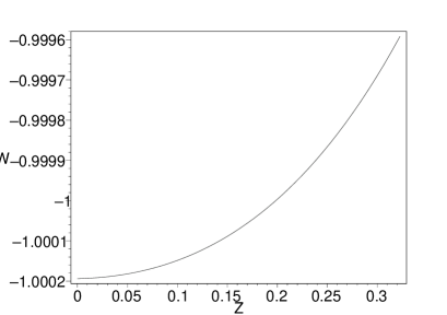
Figure 1: $w-z$ relation.

IX conclusion and discussion

The dilaton action Eq.(2) corresponds to a scalar-tensor theory in the Einstein frame, where the nonminimal coupling between scalar and Maxwell fields arises from a conformal transformation that brings the action from the Jordan to the Einstein frame. So the charged dilaton black hole resembles solutions already known in the literature. However, the phantom field considered by us is truly different because of the negative kinetic energy. Using this phantom field, we have constructed the exact solutions of electrically charged phantom black holes with the cosmological constant. The corresponding phantom potential is also obtained. The couplings between scalars and electromagnetic fields are not too surprising in high energy physics and they have been considered in observations. For example, Carroll etc have studied the astrophysical constraints on this coupling by using of the measurements of the polarization angle and orientation of cosmological radio sources [24]. On the other hand, Webb, Hannestad, Anchordoqui etc have considered the astrophysical constraints on the variation of fine structure constant using these couplings [25].
    We note that Bronnikov et al have investigated the physics of neutral phantom black holes and present some interesting results [26]. We found that the phantom field has important consequences on the properties of black holes. For large coupling constant, a small amount of electrical charge would make remarkable change on the structure of spacetime. In particular, the extremal charged phantom black holes can never be achieved and so the third law of thermodynamics for black holes is remedied. Due to the phantom charge contributes an extra repulsive force to physical mass, the phantom black hole scatters the surrounding matter while the dilaton black hole accretes the surrounding matter in our expanding Universe. This point is indicated once more in the solution for black holes in the presence of both phantom and dilaton. We also found an interior solution of a electrically charged fluid ball immersing in the phantom field. The solution shows that if we compress the mass $M$ and the phantom charge $P$ in a critical radius $r_{min}$, there will need infinite pressures at the center to against the gravity. In other words, the ball will inevitably collapse and form a phantom black hole. In the end, we point out that the quintom model for dark energy can be realized in the presence of both dilaton and phantom.

References

• (1) J. L. Tonry et al., astro-ph/0305008
• (2) R.R. Caldwell, Phys.Lett. B545 23(2002); Nojiri and S.D. Odintsov,Phys. Rev. D70,103522,2004.
• (3) V. Sahni and A. A. Starobinsky, Int. J. Mod. Phys. D9 373(2002)
• (4) L. Parker and A. Raval, Phys. Rev. D60 063512(1999)
• (5) T. Chiba, T. Okabe and M. Yamaguchi, Phys. Rev. D62 023511(2000)
• (6) B. Boisseau, G. Esposito-Farese, D. Polarski and A. A. Starobinsky, Phys. Rev. Lett.85 2236, (2000)
• (7) A. E. Schulz, Martin White, Phys.Rev. D64 043514(2001)
• (8) V. Faraoni, Int. J. Mod. Phys. D64 043514 (2002)
• (9) I. Maor, R. Brustein, J. Mcmahon and P. J. Steinhardt, Phys. Rev. D65 123003(2002)
• (10) V. K. Onemli and R. P. Woodard, Class. Quant. Grav. 19 4607(2002)
• (11) D. F. Torres, Phys. Rev. D66 043522 (2002)
• (12) S. M. Carroll, M. Hoffman, M. Trodden, astro-ph/0301273; V. K. Onemli and R. P. Woodard, Phys. Rev. D70 107301(2004); T. Brunier, V. K. Onemli and R. P. Woodard, Class. Quant. Grav. 22 59 (2005).
• (13) P. H. Frampton, Stability Issues for w Β‘ .1 Dark Energy, hep-th/0302007
• (14) J. G. Hao and X. Z. Li, gr-qc/0302100, to be published in Phys. Rev. D; X. Z. Li and J. G. Hao, hep-th/0303093.
• (15) R. R Caldwell, M. Kamionkowski and N. N. Weinberg, astro-ph/0302506; S. Nojiri, S.D. Odintsov and S. Tsujikawa, Phys. Rev. D 71,063004,2005.
• (16) G. W. Gibbons, hep-th/0302199; J.M.Cline, S. Y. Jeon and G. D.Moore, Phys. Rev. D 70, 043543 (2004).
• (17) S. Nojiri and S. D. Odintsov, hep-th/0303117; hep-th/0306212; E.Elizalde, S. Nojiri and S.D. Odintsov, hep-th/0405034; A. Feinstein and S. Jhingan, hep-th/0304069; L. P. Chimento and A. Feinstein, 11 astro-ph/0305007; P. Singh, M. Sami and N. Dadhich, hep-th/0305110; B. Wang, Y. G. Gong and E. Abdalla, hep-th/0506069; R. G. Cai and A. Z. Wang, JCAP 0503 002 (2005); R. G. Cai, H. S. Zhang and A. Z. Wang, hep-th/0505186; B. Feng, X. L. Wang and X. M. Zhang, Phys.Lett. B607 35 (2005); M. Z. Li, B. Feng and X. M. Zhang, hep-ph/0503268; Z. Y. Sun and Y. G. Shen, Gen. Rel. Grav. 37, 243 (2005).
• (18) C. J. Gao and S. N. Zhang, Phys. Lett. B605, 185 (2004).
• (19) C. J. Gao and S. N. Zhang, Phys. Lett. B617, 127 (2005)
• (20) G. W. Gibbons and K. Maeda, Nucl. Phys. B 298 (1988) 741; D. Garfinkle, G. Horowitz, A. Strominger, Phys. Rev. D 43 (1991) 3140; J. H. Horn, G. Horowitz, Phys. Rev. D 46 (1992) 1340; D. Brill, G. Horowitz, Phys. Lett. B 262 (1991) 437; R. Gregory, J. Harvey, Phys. Rev. D 47 (1993) 2411; T. Koikawa, M. Yoshimura, Phys. Lett. B 189 (1987) 29; D. Boulware, S. Deser, Phys. Lett. B 175 (1986) 409; M. Rakhmanov, Phys. Rev. D 50 (1994) 5155; R. G. Cai and Y. Z. Zhang, Phys. Rev. D 64 (2001) 104015; R. G. Cai and Y. Z. Zhang, Phys. Rev. D 54 (1996) 4891. K. C. K. Chan, J. H. Horn and R. B. Mann, Nucl. Phys. B 447 (1995) 441; G. Clement and C. Leygnac, Phys. Rev. D 70 (2004) 084018; S. J. Poletti, D. L. Wiltshire, Phys. Rev. D 50 (1994) 7260; S. J. Poletti, J. Twamley and D. L. Wiltshire, Phys. Rev. D 51 (1995) 5720; S. Mignemi and D. L. Wiltshire, Phys. Rev. D 46 (1992) 1475.
• (21) G. C. McVittie, Mon. Not. R. Astron. Soc. 93, 325 (1933).
• (22) E. Babichev, V. Dokuchaev, Yu. Eroshenko, Phys. Rev. Lett. 93,021102 (2004).
• (23) A. Vikman, Phys. Rev. D71 (2005) 023515; B. Feng, M. Li, Y. S. Piao and X. Z. Zhang, Phys. Lett. B634 (2006) 101; Z. K. Guo, Y. S. Piao et al, Phys. Lett. B608 177 (2005); M. Li, B. Feng, X. Zhang, JCAP 0512 (2005) 002; A. Anisimov, E. Babichev, A. Vikman, JCAP 0506 (2005) 006.
• (24) S. M. Carroll, Phys. Rev. Lett. 81 (1998) 3067; S. M. Carroll and G. B. Field, Phys. Rev. Lett. 79 (1997) 2394; S. M. Carroll, G. B. Field, and R. Jackiw, Phys. Rev. D41 (1990) 1231; S. M. Carroll and G. B. Field, Phys. Rev. D 43, 3789 (1991) 3789.
• (25) J. K. Webb etc, Phys. Rev. Lett. 82 (1999) 884; S. Hannestad, Phys. Rev. D60 (1999)023515; L. Anchordoqui and H. Goldberg, Phys. Rev. D68 (2003) 083513.
• (26) K. A. Bronnikov, J. C. Fabris, gr-qc/0511109.