CQUeST-2006-0026

The false vacuum bubble nucleation due to a nonminimally coupled scalar field

$\rm{Wonwoo\,\,Lee}^{\S}$   $\rm{Bum-Hoon\,\,Lee}^{{\dagger}\S}$   $\rm{Chul\,\,H.\,Lee}^{{\ddagger}}$   $\rm{Chanyong\,\,Park}^{\S}$

†Department of Physics, Sogang University, 121-742, Seoul, Korea
§Center for Quantum Spacetime, Sogang University, 121-742, Seoul, Korea
‡Department of Physics, Hanyang University, 133-791, Seoul, Korea

Abstract

We study the possibility of forming the false vacuum bubble nucleated within the true vacuum background via the true-to-false vacuum phase transition in curved spacetime. We consider a semiclassical Euclidean bubble in the Einstein theory of gravity with a nonminimally coupled scalar field. In this paper we present the numerical computations as well as the approximate analytical computations. We mention the evolution of the false vacuum bubble after nucleation.

1 Introduction

What did the spacetime look like in the very early universe? Probably there was a dynamical spacetime foam structure which was introduced by John A. Wheeler, indicating that quantum fluctuations come into play at the Planck scale, changing topology and metric [1]. Also the cosmological constant, as a dynamical variable rather than a universal constant [2], may have played an important role as an ingredient which caused a dynamical spacetime foam structure in the very early universe. But such a phenomenon is difficult to describe in the theory of gravity. On the other hand, there were investigations on the mechanism of creating the inflationary universe in the laboratory [3]. However there is no regular method for the nucleation of small regions of false vacuum. In this paper we show that such complicated vacuum structure (spacetime structure) or false vacuum bubble can occur by the vacuum-to-vacuum phase transition in the semiclassical approximation.

It has been shown that the first-order vacuum phase transitions occur via the nucleation of true vacuum bubble at zero temperature both in the absence of gravity [4] and in the presence of gravity [5]. This result was extended by Parke [6] to the case of arbitrary vacuum energy densities. An extension of this theory to the case of non-zero temperatures has been found by Linde [7] in the absence of gravity, where one should look for the $O(3)$-symmetric solution due to periodicity in the time direction $\beta$ with period $T^{-1}$ unlike the $O(4)$-symmetric solution in the zero temperature. These processes as cosmological applications of false vacuum decay have been applied to various inflationary universe scenarios by many authors [8].

As for the false vacuum bubble formation, Lee and Weinberg [9] have shown that if the vacuum energies are greater than zero, gravitational effects make it possible for bubbles of a higher-energy false vacuum to nucleate and expand within the true vacuum bubble in the de Sitter space which has a topology of 4-sphere. The false vacuum bubble nucleation is described as the inverse process of the true vacuum bubble nucleation. However, their solution is larger than the true vacuum horizon [10]. The oscillating bounce solutions, another type of Euclidean solutions, have been studied in detail by Hackworth and Weinberg [11]. On the other hand Kim et al. [13] have shown that false vacuum region may nucleate within the true vacuum bubble as global monopole bubble in the high temperature limit.

In this paper we present that the false vacuum bubble can be nucleated within the true vacuum background in the Einstein theory of gravity with a nonminimally coupled scalar field. The nonminimal coupling between a scalar field and gravity has been discussed in various cosmological scenarios such as inflation [16] and quintessence [17]. The nonminimally coupled scalar field was introduced by Chernikov and Tagirov in the context of radiation problems [20]. Other works with a nonminimal coupling term are discussed in Ref. [21], [22] and references therein.

In the semiclassical approximation, the vacuum-to-vacuum phase transition rate per unit time per unit volume is given by

$$\Gamma/V=Ae^{-B/\hbar}[1+{\cal O}(\hbar)],$$ (1)

where the pre-exponential factor $A$ is discussed in Refs. [23] and the exponent $B$ is the Euclidean action. The standard approach to the calculation of bubble nucleation rates during the first order phase transition is based on the work of Langer in statistical physics [14], and a theory of the decay of the false vacuum in spontaneously broken theories at zero temperature has been first suggested by Voloshin, Kobzarev, and Okun [15]. The standard results obtained by Coleman-De Luccia and Parke were extended to the case of the nonminimal coupling term [18], where the influence on the true vacuum bubble radius and the nucleation rates was evaluated.

How can the false vacuum bubble be nucleated within the true vacuum background via the true-to-false vacuum phase transition in the context of gravity theory? The mechanism is not known in curved spacetime with arbitrary vacuum energy in the pure Einstein theory of gravity. In this work, we study the possibility of the false vacuum bubble nucleation due to the nonminimal coupling of the scalar field $\Phi$ to the Ricci curvature using Coleman-De Luccia’s semiclassical instanton approximation. We present the numerical results as well as the approximate analytical computations.

The plan of this paper is as follows. In section 2 we present the formalism for the false vacuum bubble nucleation within the true vacuum background in the Einstein theory of gravity with a nonminimally coupled scalar field and our main idea for this work. In section 3 the numerical solutions are obtained by solving the Euclidean equation of motion of a scalar field in our model. Our solutions represent the nucleation of small regions of false vacuum bubble in curved spacetime with arbitrary vacuum energies. In section 4 the exponent $B$ and the radius of the false vacuum bubble are obtained analytically by employing Coleman’s thin-wall approximation in cases both of the false vacuum bubble nucleation within the true vacuum background and of the true vacuum bubble nucleation within the false vacuum background. In addition, we analyze the evolution of the bubble after its nucleation. The results are discussed.

2 The false vacuum bubble nucleation in the Einstein theory of gravity with a nonminimally coupled scalar field

In this section, we summarize the basic mechanism following the work presented in Ref. [18] with the correction of an error term there and present the formalism for the nucleation of false vacuum bubble within the true vacuum background with a nonminimally coupled scalar field in our model. For this theory, the action is given by

$$S=\int\sqrt{g}\>d^{4}x\left[\frac{R}{2\kappa}-\frac{1}{2}{\nabla^{\alpha}}\Phi{\nabla_{\alpha}}\Phi-\frac{1}{2}\xi R\Phi^{2}-U(\Phi)\right]+S_{b},$$ (2)

where $\kappa\equiv 8\pi G$, $g\equiv-detg_{\mu\nu}$, $U(\Phi)$ is the scalar field potential, $R$ denotes the Ricci curvature of spacetime, the term $-\xi R\Phi^{2}/2$ describes the nonminimal coupling of the field $\Phi$ to the Ricci curvature and $\xi$ is a dimensionless coupling constant. Hereafter we will omit the boundary term [19], $S_{b}$, because it will be cancelled in these processes.

Let us consider the case where $U(\Phi)$ has the form

$$U(\Phi)=\frac{\lambda}{8}\Phi^{2}(\Phi-2b)^{2}-\frac{\epsilon}{2b}(\Phi-2b)+U_{o},$$ (3)

where $\lambda$, $\epsilon$ and $b$ are positive parameters. The minimum of the potential plays the role of the cosmological constant term, and the potential $U(\Phi)$ has two nondegenerate minima, one of which is lower than the other. $U(\Phi_{T})$ corresponds to the true vacuum state and $U(\Phi_{F})$ to the false vacuum state, separated by a potential barrier (Fig. 1). These vacuum states will be modified by the nonminimally coupled scalar field, as is further discussed later.

Figure 1: Potential with two minima, $U(\phi_{F})=U_{o}+\epsilon$ and $U(\phi_{T})=U_{o}$.

The corresponding equation satisfied by the scalar field is written by

$$\frac{1}{\sqrt{g}}\partial_{\mu}[\sqrt{g}g^{\mu\nu}\partial_{\nu}\Phi]-\xi R\Phi-\frac{\partial U}{\partial\Phi}=0.$$ (4)

The Einstein equations are

$$R_{\mu\nu}-\frac{1}{2}g_{\mu\nu}R=\kappa T_{\mu\nu},$$ (5)

where $R_{\mu\nu}$ is the Ricci tensor and $T_{\mu\nu}$ is the matter energy momentum tensor,

$$T_{\mu\nu}=\frac{1}{1-\xi\Phi^{2}\kappa}\left[\nabla_{\mu}\Phi\nabla_{\nu}\Phi-g_{\mu\nu}\left(\frac{1}{2}\nabla^{\alpha}\Phi\nabla_{\alpha}\Phi+U(\Phi)\right)\right.$$

$$\left.+\xi(g_{\mu\nu}\nabla^{\alpha}\nabla_{\alpha}\Phi^{2}-\nabla_{\mu}\nabla_{\nu}\Phi^{2})\right].$$ (6)

The curvature scalar is given by

$$R=\frac{\kappa[4U(\Phi)+\nabla^{\mu}\Phi\nabla_{\mu}\Phi-3\xi\nabla^{\mu}\nabla_{\mu}\Phi^{2}]}{1-\xi\Phi^{2}\kappa}.$$ (7)

Here we adopt the notations and sign conventions of Misner, Thorne, and Wheeler [24].

$O(4)$ symmetric bubbles have the minimum Euclidean action in the absence of gravity [25] and seem to be a reasonable assumption in the presence of gravity. In our work, we assume the $O(4)$ symmetry for both $\Phi$ and the spacetime metric $g_{\mu\nu}$ in a similar manner. The most general rotationally invariant Euclidean metric is

$$ds^{2}=d\eta^{2}+\rho^{2}(\eta)[d\chi^{2}+\sin^{2}\chi(d\theta^{2}+\sin^{2}\theta d\phi^{2})].$$ (8)

Then $\Phi$ is a function of $\eta$ only and one has $R_{E}=-6(\rho^{\prime 2}+\rho\rho^{\prime\prime}-1)/\rho^{2}$. The Euclidean action becomes

$$S_{E}=2\pi^{2}\int\rho^{3}(\eta)d\eta\left[\frac{3}{\kappa}\left\{\left(\frac{\rho^{\prime}}{\rho}\right)^{2}+\left(\frac{\rho^{\prime\prime}}{\rho}\right)-\left(\frac{1}{\rho}\right)^{2}\right\}(1-\xi\Phi^{2}\kappa)+\frac{1}{2}\Phi^{\prime 2}+U(\Phi)\right],$$ (9)

where the prime denotes the differentiation with respect to $\eta$. The Euclidean field equations for $\Phi$ and $\rho$ turn out to be

$$\Phi^{\prime\prime} + \frac{3\rho^{\prime}}{\rho}\Phi^{\prime}-\xi R_{E}\Phi=\frac{dU}{d\Phi},$$ (10)

$$\rho^{\prime 2} = 1+\frac{\kappa\rho^{2}}{3(1-\xi\Phi^{2}\kappa)}(\frac{1}{2}\Phi^{\prime 2}-U),$$ (11)

respectively. The boundary conditions for the bounce are

$$\lim_{\eta\rightarrow\eta_{max}}\Phi(\eta)=\Phi_{T},\,\,\,\,\frac{d\Phi}{d\eta}\Big{|}_{\eta=0}=0.$$ (12)

where $\eta_{max}$ is a finite value in Euclidean de Sitter space and $\eta_{max}=\infty$ in both Euclidean flat and anti-de Sitter space.

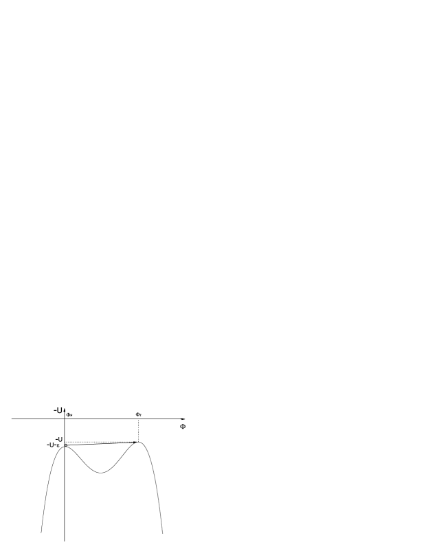
Figure 2: One-particle dynamics in the potential $-U$ .

Eq. (10) can be treated as a one-particle equation of motion with $\eta$ playing the role of time in the corresponding potential well, $-U(\Phi)$ (Fig. 2). Multiplying Eq. (10) by $\frac{d\Phi}{d\eta}$ and rearranging the terms, one obtains

$$\frac{d}{d\eta}\left[\frac{1}{2}\Phi^{\prime 2}-U\right]=-\frac{3\rho^{\prime}}{\rho}\Phi^{\prime 2}+\xi R_{E}\Phi\Phi^{\prime}.$$ (13)

The quantity in the square brackets here can be interpreted as the total energy of the particle with the potential energy $-U$, the first term on the right hand side as the dissipation rate of the total energy and the second term as the extra source of the power which appears due to coupling to gravity. The second term, as the extra power, plays an important role for the particle to reach at $-U(\Phi_{T})$. The true vacuum bubble nucleation within the false vacuum background corresponds to the particle starting at some point near $\Phi_{T}$ at $\eta=0$ and reaching $\Phi_{F}$ at $\eta=\eta_{max}$. On the other hand, the false vacuum bubble nucleation within the true vacuum background corresponds to the particle starting at some point near $\Phi_{F}$ at $\eta=0$ and reaching $\Phi_{T}$ at $\eta=\eta_{max}$. It will be possible that the false vacuum bubbles nucleate within the true vacuum background in the theory of gravity with such a term. The main idea is simple. It will happen if and only if such a term could overcome the second term on the left hand side of Eq. (10) during the phase transition,

$$\xi R_{E}\Phi>\frac{3\rho^{\prime}}{\rho}\Phi^{\prime}.$$ (14)

The second term on the left hand side of Eq. (10) is interpreted as a viscous damping term both in Euclidean flat and anti-de Sitter space. In Euclidean de Sitter space, the term is interpreted as a viscous damping term from $\rho=0$ to $\rho=\rho_{max}$ and an accelerating term from $\rho=\rho_{max}$ to $\rho=0$ because the coefficient becomes negative. To understand the role of the third term on the left hand side of Eq. (10), we can absorb $\Phi^{\prime}$-independent term into the effective potential. After the curvature scalar is substituted in Eq. (10) the field equation becomes

$${\Phi^{\prime\prime}}+\frac{3{\rho^{\prime}}}{{\rho}}\Phi^{\prime}-\frac{\xi(1-6\xi){\kappa}{\Phi^{\prime}}^{2}{\Phi}}{(1-\xi{\Phi}^{2}{\kappa}+6\xi^{2}{\Phi}^{2}{\kappa})} = \frac{1-\xi{\Phi}^{2}{\kappa}}{(1-\xi{\Phi}^{2}{\kappa}+6\xi^{2}{\Phi}^{2}{\kappa})}\frac{d{U}}{d{\Phi}}+\frac{4\xi{\Phi}{\kappa}{U}}{(1-\xi{\Phi}^{2}{\kappa}+6\xi^{2}{\Phi}^{2}{\kappa})},$$ (15)

$$= \frac{d{U}_{eff}}{d{\Phi}}.$$

The third term on the left hand side of Eq. (15) is nonlinear in $\Phi^{\prime}$, and can be interpreted as an accelerating term or viscous damping term depend on the signature.

The explicit form of the effective potential as well as the position of the vacuum states of the effective potential is not easy to write down in Eq. (15). The position of the false and true vacuum of $U(\Phi)$, $\Phi_{F}$ and $\Phi_{T}$, are not the same as that of $U_{eff}(\Phi)$, $\Phi^{eff}_{F}$ and $\Phi^{eff}_{T}$, because the position are dependent on $\xi$-coupling. While the magnitude of the effective potential for false and true vacuum, $U_{eff}(\Phi^{eff}_{F})$ and $U_{eff}(\Phi^{eff}_{T})$, are not the same as that of $U(\Phi_{F})$ and $U(\Phi_{T})$ because the magnitude are also dependent on the $\xi$-coupling. The nucleation of the false vacuum bubble for $U(\Phi)$ may be understood as the ”true vacuum” bubble nucleation of the effective potential $U_{eff}(\Phi)$ via Coleman’s mechanism for bubble nucleation.

In this work we consider five particular cases; (Case 1) from de Sitter space which has the true vacuum state of the lower positive energy density to de Sitter space which has the false vacuum state of the higher positive energy density, (Case 2) from flat space to de Sitter space, (Case 3) from anti-de Sitter space to de Sitter space, (Case 4) from anti-de Sitter space to flat space and (Case 5) from anti-de Sitter space which has the true vacuum state of the higher negative energy density to anti-de Sitter space which has the false vacuum state of the lower negative energy density.

In case 1, well inside the bubble where $\Phi$ remains constant at $\Phi_{F}$ and $U=U_{o}+\epsilon$, the solution for $\rho$ is $\rho=\Lambda\sin\frac{\eta}{\Lambda}$ and the metric is given by

$$ds^{2}=d\eta^{2}+\Lambda^{2}\sin^{2}\frac{\eta}{\Lambda}\{d\chi^{2}+\sin^{2}\chi(d\theta^{2}+\sin^{2}\theta d\phi^{2})\},$$ (16)

where $\Lambda=(\frac{3}{\kappa(U_{o}+\epsilon)})^{1/2}$. In the region outside the bubble where $\Phi$ remains constant at $\Phi_{T}$ and $U=U_{o}$, the solution for $\rho$ is $\rho=\Lambda_{1}\sin\frac{\eta+\delta}{\Lambda_{1}}$ and the metric is given by

$$ds^{2}=d\eta^{2}+\Lambda_{1}^{2}\sin^{2}\frac{\eta+\delta}{\Lambda_{1}}\{d\chi^{2}+\sin^{2}\chi(d\theta^{2}+\sin^{2}\theta d\phi^{2})\},$$ (17)

where $\Lambda_{1}=(\frac{3(1-4b^{2}\xi\kappa)}{\kappa U_{o}})^{1/2}$. Notice that a constant $\delta$ is introduced so that $\rho$ inside can be continuously matched at the wall to $\rho$ outside.

In case 2, well inside the bubble, the metric is the same form as Eq. (16). In the region outside, $\rho=\eta+\delta$ and the metric in this region is given by

$$ds^{2}=d\eta^{2}+(\eta+\delta)^{2}\{d\chi^{2}+\sin^{2}\chi(d\theta^{2}+\sin^{2}\theta d\phi^{2})\}.$$ (18)

In case 3, well inside the bubble, the metric is also the same form as Eq. (16) and outside the bubble, the solution for $\rho$ is $\rho=\Lambda_{2}\sinh\frac{\eta+\delta}{\Lambda_{2}}$ and the metric is given by

$$ds^{2}=d\eta^{2}+\Lambda_{2}^{2}\sinh^{2}\frac{\eta+\delta}{\Lambda_{2}}\{d\chi^{2}+\sin^{2}\chi(d\theta^{2}+\sin^{2}\theta d\phi^{2})\}.$$ (19)

where $\Lambda_{2}=(\frac{3(1-4b^{2}\xi\kappa)}{\kappa|U_{o}|})^{1/2}$.

In case 4, the metric inside the bubble is given by

$$ds^{2}=d\eta^{2}+\eta^{2}\{d\chi^{2}+\sin^{2}\chi(d\theta^{2}+\sin^{2}\theta d\phi^{2})\},$$ (20)

and outside the bubble, the metric is the same form as Eq. (19).

In case 5, the metric inside the wall is given by

$$ds^{2}=d\eta^{2}+\Lambda_{3}^{2}\sinh^{2}\frac{\eta}{\Lambda_{3}}\{d\chi^{2}+\sin^{2}\chi(d\theta^{2}+\sin^{2}\theta d\phi^{2})\},$$ (21)

where $\Lambda_{3}=(\frac{3}{\kappa(|U_{o}|-\epsilon)})^{1/2}$ and the metric outside the bubble is the same form as Eq. (19).

3 Numerical calculation

The Euclidean field equations, (10) and (11), can be solved analytically. Hence in this section we solve the equations numerically. We first rewrite the equations in terms of dimensionless variables as follows

$$\frac{\lambda U(\Phi)}{\mu^{4}}=\tilde{U}(\tilde{\Phi}),\;\;\frac{\lambda\Phi^{2}}{\mu^{2}}=\tilde{\Phi^{2}},\;\;\frac{\lambda\epsilon}{\mu^{4}}=\tilde{\epsilon},\;\;\mu\eta=\tilde{\eta},\;\;\mu\rho=\tilde{\rho}.$$ (22)

These variables give

$$\tilde{U}(\tilde{\Phi})=\frac{1}{8}\tilde{\Phi}^{2}(\tilde{\Phi}-2)^{2}-\frac{\tilde{\epsilon}}{2}(\tilde{\Phi}-2)+\tilde{U_{o}},$$ (23)

and the Euclidean field equations for $\Phi$ and $\rho$ become

$$\tilde{\Phi^{\prime\prime}} + \frac{3\tilde{\rho^{\prime}}}{\tilde{\rho}}\tilde{\Phi^{\prime}}-\xi\tilde{R}_{E}\tilde{\Phi}=\frac{d\tilde{U}}{d\tilde{\Phi}},$$ (24)

$$\tilde{\rho^{\prime}}^{2} = 1+\frac{\tilde{\kappa}\tilde{\rho}^{2}}{3(1-\xi\tilde{\Phi}^{2}\tilde{\kappa})}(\frac{1}{2}\tilde{\Phi^{\prime}}^{2}-\tilde{U}),$$ (25)

respectively, where $\tilde{R}_{E}=R_{E}/\mu^{2}$, $\tilde{\rho}=\rho\mu$ and $\tilde{\kappa}=\frac{\mu^{2}}{\lambda}\kappa$. The boundary conditions also become

$$\lim_{\tilde{\eta}\rightarrow\tilde{\eta}_{max}}\tilde{\Phi}(\tilde{\eta})=\tilde{\Phi}_{T},\,\,\,\,\frac{d\tilde{\Phi}}{d\tilde{\eta}}\Big{|}_{\tilde{\eta}=0}=0.$$ (26)

Figure 3: The false vacuum bubble profiles for several values of $\tilde{\epsilon}$ and $\xi$ in case 1. Here $\xi$ is taken to be positive value. The three curves are (a) solid curve: $\tilde{\epsilon}=0.01$ and $\xi\simeq 0.271$, (b) dotted curve: $\tilde{\epsilon}=0.02$ and $\xi\simeq 0.313$, (c) dashed curve: $\tilde{\epsilon}=0.03$ and $\xi\simeq 0.346$. Hereafter the axes denote the tilde attached variables.

In this work we consider the five particular cases of true-to-false vacuum phase transitions; (Case 1) from de Sitter space to de Sitter space, (Case 2) from flat space to de Sitter space, (Case 3) from anti-de Sitter space to de Sitter space, (Case 4) from anti-de Sitter space to flat space and (Case 5) from anti-de Sitter space to anti-de Sitter space.

In Case 1, a scalar field originally in the true vacuum state of the lower positive energy density decays into the false vacuum state of the higher positive energy density. We have computed three cases of bubble profiles corresponding to (a) solid curve: $\tilde{\epsilon}=0.01$ and $\xi\simeq 0.271$, (b) dotted curve: $\tilde{\epsilon}=0.02$ and $\xi\simeq 0.313$, (c) dashed curve: $\tilde{\epsilon}=0.03$ and $\xi\simeq 0.346$ and we take $\tilde{\kappa}=0.3,\tilde{U_{T}}=0.01$. We can see from the Fig. 3 that the radius of bubble becomes larger as $\tilde{\epsilon}$ becomes smaller. But in order to climb the hill, $U_{eff}(\Phi^{eff}_{T})$, the value of $\xi$ becomes larger as $\tilde{\epsilon}$ becomes larger. This can be understood because $\xi$-term acts as an accelerating term which helps the particle to climb the hill, up to $U_{eff}(\Phi^{eff}_{T})$. The evolution of $\tilde{\rho}(\tilde{\eta})$ is shown in Fig. 4. The solid curve is the solution of $\tilde{\rho}$ with $\tilde{\epsilon}=0.01$. In the region inside the bubble, $\rho=\Lambda\sin\frac{\eta}{\Lambda}$, and outside the bubble, $\rho=\Lambda_{1}\sin\frac{\eta+\delta}{\Lambda_{1}}$. Here we obtain the small region of the false vacuum bubble within the true vacuum background which is de Sitter space. The bending part of the solid curve corresponds to the bubble wall. The thick bubble wall exists when the difference in energy density between the false and true vacuum is large.

Figure 4: The evolution of $\tilde{\rho}(\tilde{\eta})$ in case 1. The solid curve is the solution of $\tilde{\rho}$ with $\tilde{\epsilon}=0.01$. In the region inside the bubble, $\rho=\Lambda\sin\frac{\eta}{\Lambda}$, and outside the bubble, $\rho=\Lambda_{1}\sin\frac{\eta+\delta}{\Lambda_{1}}$.

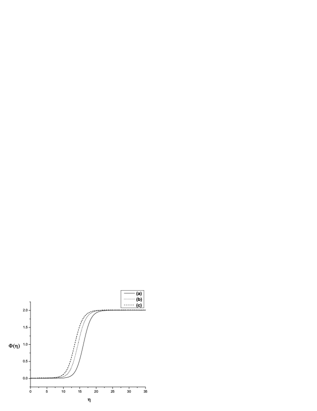
Figure 5: The false vacuum bubble profiles for several values of $\tilde{\epsilon}$ and $\xi$ in case 2. Here $\xi$ is taken to be positive. The three curves are (a) solid curve: $\tilde{\epsilon}=0.01$ and $\xi\simeq 0.311$, (b) dotted curve: $\tilde{\epsilon}=0.02$ and $\xi\simeq 0.360$, (c) dashed curve: $\tilde{\epsilon}=0.03$ and $\xi\simeq 0.396$.

In Case 2, the true vacuum state with the zero energy density decays into the false vacuum state with the positive energy density. We have computed three cases in the similar manner to Case 1. The corresponding results are presented by (a) solid curve: $\tilde{\epsilon}=0.01$ and $\xi\simeq 0.311$, (b) dotted curve: $\tilde{\epsilon}=0.02$ and $\xi\simeq 0.360$, (c) dashed curve: $\tilde{\epsilon}=0.03$ and $\xi\simeq 0.396$ and we also take $\tilde{\kappa}=0.3,\tilde{U_{T}}=0$ (Fig. 5). The solid curve is the solution of $\tilde{\rho}$ with $\tilde{\epsilon}=0.01$ (Fig. 6). In the region inside the bubble, $\rho=\Lambda\sin\frac{\eta}{\Lambda}$, and outside the bubble, $\rho=\eta+\delta$.

In Case 3, the true vacuum state with the negative energy density decays into the false vacuum state with the positive energy density. We have computed three cases in the similar manner to Case 1. The corresponding results are (a) solid curve: $\tilde{\epsilon}=0.01$ and $\xi\simeq 0.328$, (b) dotted curve: $\tilde{\epsilon}=0.02$ and $\xi\simeq 0.414$, (c) dashed curve: $\tilde{\epsilon}=0.03$ and $\xi\simeq 0.508$ and we also take $\tilde{\kappa}=0.3$ (Fig. 7). The solid curve is the solution of $\tilde{\rho}$ with $\tilde{\epsilon}=0.01$ (Fig. 8). In the region inside the bubble, $\rho=\Lambda\sin\frac{\eta}{\Lambda}$, and outside the bubble, $\rho=\Lambda_{2}\sinh\frac{\eta+\delta}{\Lambda_{2}}$.

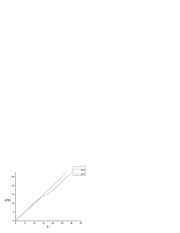
Figure 6: The evolution of $\tilde{\rho}(\tilde{\eta})$ in case 2. The solid curve is the solution of $\tilde{\rho}$ with $\tilde{\epsilon}=0.01$. In the region inside the bubble, $\rho=\Lambda\sin\frac{\eta}{\Lambda}$, and outside the bubble, $\rho=\eta+\delta$.

Figure 7: The false vacuum bubble profiles for several values of $\tilde{\epsilon}$ and $\xi$ in case 3. Here $\xi$ is taken to be positive. The three curves are (a) solid curve: $\tilde{\epsilon}=0.01$ and $\xi\simeq 0.328$, (b) dotted curve: $\tilde{\epsilon}=0.02$ and $\xi\simeq 0.414$, (c) dashed curve: $\tilde{\epsilon}=0.03$ and $\xi\simeq 0.508$.

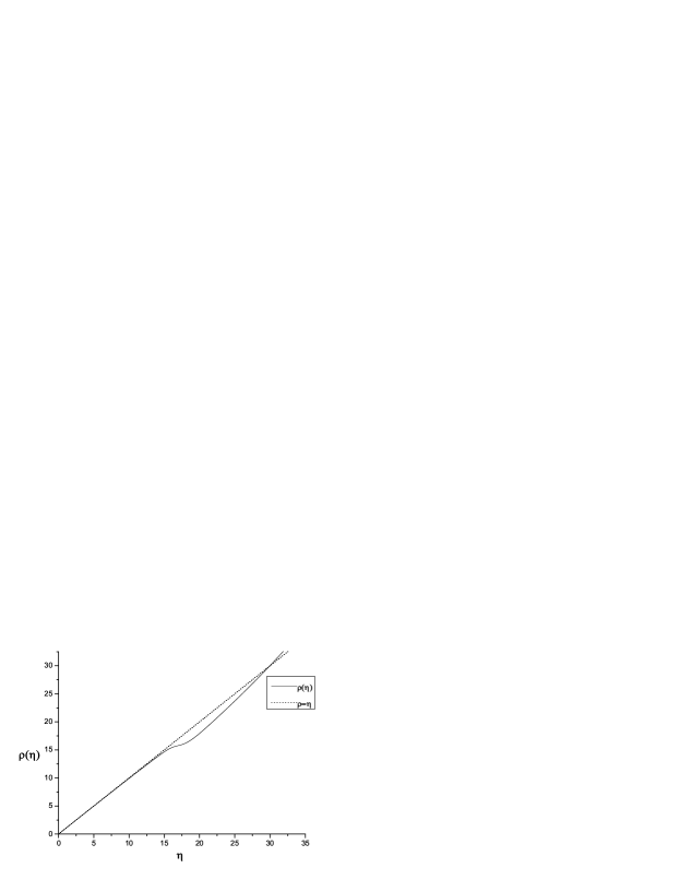
Figure 8: The evolution of $\tilde{\rho}(\tilde{\eta})$ in case 3. The solid curve is the solution of $\tilde{\rho}$ with $\tilde{\epsilon}=0.01$. In the region inside the bubble, $\rho=\Lambda\sin\frac{\eta}{\Lambda}$, and outside the bubble, $\rho=\Lambda_{2}\sinh\frac{\eta+\delta}{\Lambda_{2}}$.

In Case 4, the true vacuum state with the negative energy density decays into the false vacuum state with the zero energy density. The results are (a) solid curve: $\tilde{\epsilon}=0.01$ and $\xi\simeq 0.258$, (b) dotted curve: $\tilde{\epsilon}=0.015$ and $\xi\simeq 0.316$, (c) dashed curve: $\tilde{\epsilon}=0.02$ and $\xi\simeq 0.377$ and we also take $\tilde{\kappa}=0.3,\tilde{U_{F}}=0$ (Fig. 9). The solid curve is the solution of $\tilde{\rho}$ with $\tilde{\epsilon}=0.01$ (Fig. 10). In the region inside the bubble, $\rho=\eta$, and outside the bubble, $\rho=\Lambda_{2}\sinh\frac{\eta+\delta}{\Lambda_{2}}$.

Figure 9: The false vacuum bubble profiles for several values of $\tilde{\epsilon}$ and $\xi$ in case 4. Here $\xi$ is taken to be positive. The three curves are (a) solid curve: $\tilde{\epsilon}=0.01$ and $\xi\simeq 0.258$, (b) dotted curve: $\tilde{\epsilon}=0.015$ and $\xi\simeq 0.316$, (c) dashed curve: $\tilde{\epsilon}=0.02$ and $\xi\simeq 0.377$.

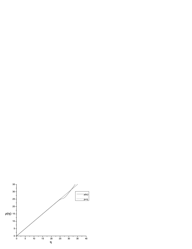
Figure 10: The evolution of $\tilde{\rho}(\tilde{\eta})$ in case 4. The solid curve is the solution of $\tilde{\rho}$ with $\tilde{\epsilon}=0.01$. In the region inside the bubble, $\rho=\eta$, and outside the bubble, $\rho=\Lambda_{2}\sinh\frac{\eta+\delta}{\Lambda_{2}}$.

In Case 5, the true vacuum state with the higher negative energy density decays into the false vacuum state with the lower negative energy density. We have computed three cases in the similar manner to Case 1. But here we obtain the different results from other cases. The radius of bubble is diminished as $\tilde{\epsilon}$ is diminished. The corresponding results are (a) solid curve: $\tilde{\epsilon}=0.01$ and $\xi\simeq 0.359$, (b) dotted curve: $\tilde{\epsilon}=0.005$ and $\xi\simeq 0.319$, (c) dashed curve: $\tilde{\epsilon}=0.015$ and $\xi\simeq 0.400$ and we also take $\tilde{\kappa}=0.3,\tilde{U_{F}}=-0.01$ (Fig. 11). The solid curve is the solution of $\tilde{\rho}$ with $\tilde{\epsilon}=0.01$ (Fig. 12). In the region inside the bubble, $\rho=\Lambda_{3}\sinh\frac{\eta}{\Lambda_{3}}$, and outside the bubble, $\rho=\Lambda_{2}\sinh\frac{\eta+\delta}{\Lambda_{2}}$.

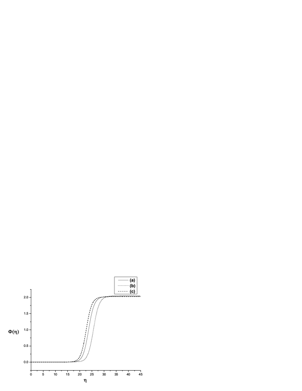
Figure 11: The false vacuum bubble profiles for several values of $\tilde{\epsilon}$ and $\xi$ in case 5. Here $\xi$ is taken to be positive. The three curves are (a) solid curve: $\tilde{\epsilon}=0.01$ and $\xi\simeq 0.359$, (b) dotted curve: $\tilde{\epsilon}=0.015$ and $\xi\simeq 0.400$, (c) dashed curve: $\tilde{\epsilon}=0.005$ and $\xi\simeq 0.319$.

Figure 12: The evolution of $\tilde{\rho}(\tilde{\eta})$ in case 5. The solid curve is the solution of $\tilde{\rho}$ with $\tilde{\epsilon}=0.01$. In the region inside the bubble, $\rho=\Lambda_{3}\sinh\frac{\eta}{\Lambda_{3}}$, and outside the bubble, $\rho=\Lambda_{2}\sinh\frac{\eta+\delta}{\Lambda_{2}}$.

In summary, we have shown that there exist parameter regions where the false vacuum bubble can be formed in all cases.

4 The thin-wall approximation

In the limit of small $\epsilon$ the field stays near to the top of the hill of the inverted potential, $-U(\Phi_{F})$, for quite a long time so that $\rho$ grows large with $\Phi$ staying near $\Phi_{F}$. As $\rho$ becomes large, the second term becomes negligible and $\Phi$ quickly goes to $\Phi_{T}$ and stays at that point from thereafter. From the Euclidean field equations for $\Phi$ and $\rho$, the second term on the left hand side of Eq. (10) is given by

$$3\frac{\rho^{\prime}}{\rho}\Phi^{\prime}=3\left[\frac{1}{\rho^{2}}+\frac{\kappa(\frac{1}{2}\Phi^{\prime 2}-U)}{3(1-\xi\Phi^{2}\kappa)}\right]\Phi^{\prime}.$$ (27)

In this section we assume the thin-wall approximation. The validity of the thin-wall approximation has been described in detail by Samuel and Hiscock [27]. However, in order to get the effect of nonminimal coupling we will keep the term in the Euclidean field equations.

In this approximation, it is justified to neglect the second term, $\frac{3\rho^{\prime}}{\rho}\Phi^{\prime}$, and the bubble nucleation rate is calculated by $\Gamma/V=Ae^{-B/\hbar}$ where $B$ is the difference between the Euclidean action of the bounce and that of the true vacuum state,

$$B=S^{b}_{E}-S^{T.V.}_{E}.$$ (28)

Thus, the Euclidean action is given by

$$S_{E} = 2\pi^{2}\int_{0}^{\infty}d\eta\left[\rho^{3}\left(\frac{1}{2}(\Phi^{\prime})^{2}+U(\Phi)\right)+\frac{3(1-\xi\Phi^{2}\kappa)}{\kappa}(\rho\rho^{\prime 2}+\rho^{2}\rho^{\prime\prime}-\rho)\right]$$ (29)

$$= 4\pi^{2}\int_{0}^{\infty}d\eta\left[\rho^{3}U(\Phi)-\frac{3\rho(1-\xi\Phi^{2}\kappa)}{\kappa}+3\xi\rho^{2}\rho^{\prime}\Phi\Phi^{\prime}\right].$$

Here we eliminate the second-derivative term by integration by parts and use the Euclidean field equation to eliminate $\rho^{\prime}$. The third term of the second line in Eq. (29) is vanished because of $\rho^{\prime}\to 0$ in the wall and $\Phi^{\prime}\to 0$ both inside and outside of the wall, respectively.

Now, we shall use the thin-wall approximation scheme to evaluate $B$. In this approximation the exponent $B$ can be divided into three parts

$$B=B_{in}+B_{wall}+B_{out}.$$ (30)

Outside the wall,

$$B_{out}=S_{E}(\Phi_{T})-S_{E}(\Phi_{T})=0.$$ (31)

In the wall, we can replace $\rho$ by $\bar{\rho}$ and Eq. (10) can be modified

$$\frac{d^{2}\Phi}{d\eta^{2}}=\frac{dU}{d\Phi}+\xi R_{E}\Phi.$$ (32)

Multiplying Eq. (10) by $\frac{d\Phi}{d\eta}$ and then integrating over $\eta$, one obtains

$$\frac{d\Phi}{d\eta}=-\sqrt{2[U(\Phi)-U(\Phi_{T})]+\xi R_{E}(\Phi^{2}-\Phi_{T}^{2})},$$ (33)

where Ricci scalar $R_{E}$ is a function of $\rho$ only in the wall and the minus sign is chosen because we are interested in the region $\Phi_{F}<\Phi<\Phi_{T}$. This minus sign is important for the positive contribution from the wall. We neglect the term $\int\xi\Phi^{2}R_{E}^{\prime}d\eta$ in the above equation because we use $R_{E}\simeq\frac{6}{\bar{\rho^{2}}}$ only in the wall in this thin-wall approximation. In this work we use the condition $d\Phi/d\eta|_{\Phi_{T}}=0$, and consider the case where $\frac{\lambda\epsilon}{\mu^{4}}$ is small and we approximate the quantity to the first order of this parameter.

Then, the contribution from the wall, $B_{wall}$, is given by

$$B_{wall} = 4\pi^{2}\bar{\rho^{3}}\int_{\Phi_{F}}^{\Phi_{T}}\left[(U(\Phi)-U(\Phi_{T}))+\frac{3}{\bar{\rho^{2}}}\xi(\Phi^{2}-\Phi_{T}^{2})\right]d\eta$$ (34)

$$= 2\pi^{2}\bar{\rho^{3}}\int_{\Phi_{T}}^{\Phi_{F}}\sqrt{2[U(\Phi)-U(\Phi_{T})]+\frac{6\xi}{\bar{\rho^{2}}}(\Phi^{2}-\Phi_{T}^{2})}d\Phi$$

$$= 2\pi^{2}\bar{\rho^{3}}\left[\int_{\Phi_{T}}^{\Phi_{F}}\sqrt{2[U(\Phi)-U(\Phi_{T})]}d\Phi-\frac{C\xi}{\bar{\rho^{2}}}\right]$$

$$= 2\pi^{2}\bar{\rho^{3}}(S_{o}-\frac{C\xi}{\bar{\rho^{2}}}),$$

where $S_{o}=\int_{\Phi_{T}}^{\Phi_{F}}\sqrt{2[U(\Phi)-U(\Phi_{T})]}d\Phi$ and $C=\frac{12b}{\sqrt{\lambda}}(1+2\ln{\frac{4b^{4}\lambda+\epsilon}{\epsilon}})$. In the third line, we approximate the quantity in the square root to the first order. The second term of the fourth line reflects the correction of Euclidean surface density.

To evaluate the Euclidean action inside the wall, we will use $d\rho=d\eta[1-\frac{\kappa\rho^{2}U}{3(1-\xi\Phi^{2}\kappa)}]$

$$B_{in}=\frac{12\pi^{2}}{\kappa^{2}}\left[\frac{(1-\xi\Phi_{F}^{2}\kappa)^{2}\{[1-\frac{\kappa\bar{\rho^{2}}U(\Phi_{F})}{3(1-\xi\Phi_{F}^{2}\kappa)}]^{3/2}-1\}}{U(\Phi_{F})}\right.$$

$$-\left.\frac{(1-\xi\Phi_{T}^{2}\kappa)^{2}\{[1-\frac{\kappa\bar{\rho^{2}}U(\Phi_{T})}{3(1-\xi\Phi_{T}^{2}\kappa)}]^{3/2}-1\}}{U(\Phi_{T})}\right]$$ . (35)

This $B_{in}$ is the contribution from inside the bubble.

To find the critical bubble size, $B$ has to be extremized with respect to $\bar{\rho}$,

$$\frac{dB}{d\bar{\rho}}=12\pi^{2}\bar{\rho}\left[\left(\frac{1-\xi\Phi_{T}^{2}\kappa}{\kappa}\right)\left(1-\frac{\kappa\bar{\rho}^{2}U(\Phi_{T})}{3(1-\xi\Phi_{T}^{2}\kappa)}\right)^{1/2}\right.$$

$$-\left.\left(\frac{1-\xi\Phi_{F}^{2}\kappa}{\kappa}\right)\left(1-\frac{\kappa\bar{\rho}^{2}U(\Phi_{F})}{3(1-\xi\Phi_{F}^{2}\kappa)}\right)^{1/2}\right]+6\pi^{2}\bar{\rho}^{2}S_{o}-2\pi^{2}C\xi=0.$$ (36)

Here we take $\Phi_{F}=0$, $\Phi_{T}=2b$, $\lambda_{1}^{2}=[3/\kappa(U_{F}+U_{T})]$ and $\lambda_{2}^{2}=[3/\kappa(U_{F}-U_{T})]$, then the radius of the false vacuum bubble is given by

$$\bar{\rho}^{2}=\frac{H\pm\sqrt{H^{2}-ED}}{E},$$ (37)

where $E=[1+2(\frac{\bar{\rho}_{o}}{2\lambda_{1}})^{2}+(\frac{\bar{\rho}_{o}}{2\lambda_{2}})^{4}]+8b^{2}\xi\kappa^{3}\lambda_{2}^{2}U_{T}\left(\frac{8b^{2}\xi U_{T}}{3}-\frac{S_{o}^{2}}{2}\right)$, $H=\frac{\bar{\rho_{o}^{2}}}{S_{o}^{2}}[(2-8b^{2}\xi\kappa)\left(\frac{S_{o}^{2}}{4}-4b^{2}\xi U_{T}\right)+\frac{\xi(U_{F}+U_{T})}{3}\left(16b^{4}\xi\kappa-8b^{2}-\frac{S_{o}C\kappa}{6}\right)]$, $D=\frac{\bar{\rho_{o}^{2}}}{S_{o}^{2}}[\xi\left(64b^{4}\xi+\frac{2S_{o}C}{3}\right)-256b^{6}\xi^{3}\kappa-\frac{8b^{2}\xi^{2}S_{o}C\kappa}{3}]$, and $\bar{\rho}_{o}=3S_{o}/[U_{F}-U_{T}]$ is the bubble size without gravity. If $\xi=0$ is substituted into Eq. (37), then the $\bar{\rho}^{2}$ is given by

$$\bar{\rho}_{p}^{2}=\frac{\bar{\rho}_{o}^{2}}{\left[1+2(\frac{\bar{\rho}_{o}}{2\lambda_{1}})^{2}+(\frac{\bar{\rho}_{o}}{2\lambda_{2}})^{4}\right]},$$ (38)

which is consistent with Parke’s results [6].

In this case the coefficient $B$ is given by

$$B = \frac{12\pi^{2}}{\kappa^{2}}\left[\frac{1}{U_{F}}\left\{\left(1-\frac{\kappa\bar{\rho^{2}}U_{F}}{3}\right)^{3/2}-1\right\}-\frac{(1-4b^{2}\xi\kappa)^{2}}{U_{T}}\left\{\left(1-\frac{\kappa\bar{\rho^{2}}U_{T}}{3(1-4b^{2}\xi\kappa)}\right)^{3/2}-1\right\}\right]$$ (39)

$$+ 2\pi^{2}\bar{\rho^{3}}\left(S_{o}-\frac{C\xi}{\bar{\rho^{2}}}\right),$$

here we take the plus sign in Eq. (37) and Eq. (41).

On the other hand, if we consider the true vacuum bubble nucleation within the false vacuum background in this model, in the wall

$$B_{1wall}=2\pi^{2}\bar{\rho_{1}^{3}}(S_{o}-\frac{C_{1}\xi}{\bar{\rho^{2}}}),$$ (40)

where $C_{1}=\frac{12b}{\sqrt{\lambda}}(1+2\ln{\frac{\epsilon}{\epsilon-4b^{4}\lambda}})$. The radius of true vacuum bubble is given by

$$\bar{\rho}_{1}^{2}=\frac{H_{1}\pm\sqrt{H_{1}^{2}-ED_{1}}}{E},$$ (41)

where $E=[1+2(\frac{\bar{\rho}_{o}}{2\lambda_{1}})^{2}+(\frac{\bar{\rho}_{o}}{2\lambda_{2}})^{4}]+8b^{2}\xi\kappa^{3}\lambda_{2}^{2}U_{T}\left(\frac{8b^{2}\xi U_{T}}{3}-\frac{S_{o}^{2}}{2}\right)$, $H_{1}=\frac{\bar{\rho_{o}^{2}}}{S_{o}^{2}}[(2-8b^{2}\xi\kappa)\left(\frac{S_{o}^{2}}{4}-4b^{2}\xi U_{T}\right)+\frac{\xi(U_{F}+U_{T})}{3}\left(16b^{4}\xi\kappa-8b^{2}-\frac{S_{o}C_{1}\kappa}{6}\right)]$, and $D_{1}=\frac{\bar{\rho_{o}^{2}}}{S_{o}^{2}}[\xi\left(64b^{4}\xi+\frac{2S_{o}C_{1}}{3}\right)-256b^{6}\xi^{3}\kappa-\frac{8b^{2}\xi^{2}S_{o}C_{1}\kappa}{3}]$ and the coefficient $B_{1}$ is given by

$$B_{1} = \frac{12\pi^{2}}{\kappa^{2}}\left[\frac{(1-4b^{2}\xi\kappa)^{2}}{U_{T}}\left\{\left(1-\frac{\kappa\bar{\rho_{1}^{2}}U_{T}}{3(1-4b^{2}\xi\kappa)}\right)^{3/2}-1\right\}-\frac{1}{U_{F}}\left\{\left(1-\frac{\kappa\bar{\rho_{1}^{2}}U_{F}}{3}\right)^{3/2}-1\right\}\right]$$ (42)

$$+ 2\pi^{2}\bar{\rho^{3}}\left(S_{o}-\frac{C_{1}\xi}{\bar{\rho^{2}}}\right).$$

If $\xi=0$ is substituted into the above equation, then the coefficient $B_{1}$ is given by

$$B_{p}=\frac{2B_{o}[\{1+(\frac{\bar{\rho_{o}}}{2\lambda_{1}})^{2}\}-\{1+2(\frac{\bar{\rho}_{o}}{2\lambda_{1}})^{2}+(\frac{\bar{\rho}_{o}}{2\lambda_{2}})^{4}\}^{1/2}]}{[(\frac{\bar{\rho_{o}}}{2\lambda_{2}})^{4}\{(\frac{\lambda_{2}}{\lambda_{1}})^{2}-1\}\{1+2(\frac{\bar{\rho}_{o}}{2\lambda_{1}})^{2}+(\frac{\bar{\rho}_{o}}{2\lambda_{2}})^{4}\}^{1/2}]},$$ (43)

where $B_{o}=27\pi^{2}S_{o}^{4}/2\epsilon^{3}$ is the nucleation rate in the absence of gravity. $B_{p}$ is obtained by Parke [6].

Now we discuss the evolution of the false vacuum bubble after its nucleation. The false vacuum bubble after its nucleation will either expand or shrink. Can the false vacuum bubble expand within the true vacuum background? It’s not a trivial problem in curved spacetime because the energy cannot be globally defined and the energy conservation does not work for vacuum energy in general. The dynamics of the false vacuum bubble or inflating regions is discussed in Refs. [28] by employing the junction condition. However, in order to progress our analysis continuously, the spacetime outside bubble will be kept flat (Minkowski), de Sitter or anti-de Sitter spacetime.

Here we analyze the growth of the bubble, following Ref. [29], where we have discussed the dynamics of true vacuum bubble. De Sitter space which includes some aspects pertaining to bubble nucleation have been described in Ref. [30]. As the first step to analyze the growth of the bubble, the Lorentzian solution is obtained by applying the analytic continuation

$$\chi\to i\chi+\frac{\pi}{2},$$ (44)

to the Euclidean solution. The only difference is that one has to continue the metric as well as the scalar field, $O(4)$-invariant Euclidean space into an $O(3,1)$-invariant Lorentzian spacetime.

In case 1, the spacetime metric inside the bubble which is obtained by applying Eq. (44) to Eq. (16) is

$$ds^{2}=d\eta^{2}+\Lambda^{2}\sin^{2}\frac{\eta}{\Lambda}\{-d\chi^{2}+\cosh^{2}\chi(d\theta^{2}+\sin^{2}\theta d\phi^{2})\},$$ (45)

and the metric outside the bubble which is given by

$$ds^{2}=d\eta^{2}+\Lambda_{1}^{2}\sin^{2}\frac{\eta+\delta}{\Lambda_{1}}\{-d\chi^{2}+\cosh^{2}\chi(d\theta^{2}+\sin^{2}\theta d\phi^{2})\},$$ (46)

which are the spatially inhomogeneous de Sitter like metrics. For Minkowski spacetime, it becomes the spherical Rindler type [31].

We next look for the static spherically symmetric forms of the metric given in Eq’s. (45) to (46). Both inside and outside the bubble, the coordinate transformation

$$r = \Lambda_{1}\sin\frac{\eta+\delta}{\Lambda_{1}}\cosh\chi,$$

$$t = \frac{\Lambda_{1}}{2}\ln\frac{\cos\frac{\eta+\delta}{\Lambda_{1}}+\sin\frac{\eta+\delta}{\Lambda_{1}}\sinh\chi}{\cos\frac{\eta+\delta}{\Lambda_{1}}-\sin\frac{\eta+\delta}{\Lambda_{1}}\sinh\chi},$$ (47)

change the metric to

$$ds^{2} = -\left(1-\frac{r^{2}}{\Lambda^{2}}\right)dt^{2}+\frac{dr^{2}}{1-\frac{r^{2}}{\Lambda^{2}}}+r^{2}(d\theta^{2}+\sin^{2}\theta d\phi^{2}),$$

$$ds^{2} = -\left(1-\frac{r^{2}}{\Lambda_{1}^{2}}\right)dt^{2}+\frac{dr^{2}}{1-\frac{r^{2}}{\Lambda_{1}^{2}}}+r^{2}(d\theta^{2}+\sin^{2}\theta d\phi^{2}),$$ (48)

respectively, which are the static spherically symmetric forms of the de Sitter metric. The region of the bubble wall cannot be represented by a static spherically symmetric metric. However, when the wall width is very small so that the thin wall approximation is valid, almost all of the entire space except the thin bubble wall region can be approximately represented by static spherically symmetric metrics. The middle of the bubble wall can be considered to be located at some constant value of $\eta$, say $\bar{\eta}$, in the coordinate system of Eq. (8). Now let us consider a spacetime point corresponding to a constant value of $\eta$, say $\eta_{c}$, which is close to $\bar{\eta}$, but still within the region that can approximately be represented by a static spherically symmetric metric. Tracing the motion of this point is then almost the same as tracing the motion of the bubble wall. We now proceed to trace the motion of such a point just inside or outside the bubble wall. For a point just inside the bubble wall in case 1, we differentiate Eq. (47) with respect to $\chi$ keeping $\eta$ constant as $\eta=\eta_{c}$ to obtain

$$dr = \Lambda_{1}\sin\frac{\eta_{c}+\delta}{\Lambda_{1}}\sinh\chi d\chi,$$

$$dt = \Lambda_{1}\frac{\sin\frac{\eta_{c}+\delta}{\Lambda_{1}}\cos\frac{\eta_{c}+\delta}{\Lambda_{1}}\cosh\chi}{1-\sin^{2}\frac{\eta_{c}+\delta}{\Lambda_{1}}\cosh^{2}\chi}d\chi,$$

$$d\tau = \pm\sqrt{(1-\frac{r^{2}}{\Lambda_{1}^{2}})dt^{2}-\frac{dr^{2}}{(1-\frac{r^{2}}{\Lambda_{1}^{2}})}}.$$ (49)

The growth rate of the bubble wall radius per unit proper time seen from outside the wall is then calculated to be approximately

$$\frac{dr}{d\tau}=\sqrt{\frac{r^{2}}{r_{o}^{2}}-1},$$ (50)

where $r_{o}=\Lambda_{1}\sin\frac{\eta_{c}+\delta}{\Lambda_{1}}$ is the value of $r$ at $t=0(\chi=0)$. Here we take the positive value because the quantity must be the positive value in the square root, that is to say, it represents the expansion of the false vacuum bubble and also repulsive nature [32]. The $d\tau$ goes to zero as the bubble wall becomes large, so the proper velocity has a large value. We can also obtain the same form inside the bubble wall. Furthermore, we can obtain the same form in every other cases (see Ref. [29]). In future work we will discuss further the dynamics of the false vacuum bubble by employing the junction condition.

5 Summary and Discussions

In this paper we have shown that the false vacuum bubble can be nucleated within the true vacuum background in the Einstein theory of gravity with a nonminimally coupled scalar field by solving the Euclidean field equations of motion in the semiclassical approximation.

In section 2 we have presented the formalism for the false vacuum bubble nucleation within the true vacuum background and our main idea for this work.

In section 3 we have considered the true-to-false vacuum phase transitions in the five particular cases; (Case 1) from de Sitter space to de Sitter space, (Case 2) from flat space to de Sitter space, (Case 3) from anti-de Sitter space to de Sitter space, (Case 4) from anti-de Sitter space to flat space and (Case 5) from anti-de Sitter space to anti-de Sitter space. We have obtained numerical solutions. In case 1, we have obtained the false vacuum smaller than the true vacuum horizon. The case 3 can be interesting from the aspect of the so-called string landscape [33], which has included both anti-de Sitter and de Sitter minima [34]. Our solution represent how the false vacuum bubble, corresponding to the de Sitter spacetime, can be nucleated within the true vacuum background, corresponding to the anti-de Sitter spacetime.

The thick bubble wall exists when the difference in energy density between the false and true vacuum is large. For the infinitely thick bubble wall, the Hawking-Moss transition has been known [12] and discussed in Refs. [26] although the transition is certainly not evident from the thin-wall study of Coleman and De Luccia.

In section 4 we obtained the exponent $B$ and the radius of the false vacuum bubble approximately by employing Coleman’s thin-wall approximation in the cases both the false vacuum bubble nucleation within the true vacuum background and the true vacuum bubble nucleation within the false vacuum background.

If the vacuum-to-vacuum phase transitions occur one after another, false-to-true and true-to-false, the whole spacetime will have the complicated vacuum or spacetime structure like as an onion with different number of the coats everywhere. The black hole creation [35] in our model may make the whole spacetime more chaotic one.

In addition, using the analytic continuation we have discussed the evolution of the false vacuum bubble in Lorentzian spacetime. Here we have shown that the proper circumferential radius of the bubble wall grows according to $\frac{dr}{d\tau}=\sqrt{\frac{r^{2}}{r_{o}^{2}}-1}$ both inside and outside the wall in thin-wall approximation. The $d\tau$ goes to zero as the bubble wall becomes large.

In fact, in order to analyze more precisely the spacetime outside the bubble, we need to take the Schwarzschild or Schwarzschild-de Sitter (anti-de Sitter) spacetime [36] by Birkhoff’s theorem [37] although one can not obtain the Schwarzschild or Schwarzschild-de Sitter (anti-de Sitter) spacetime from Eq. (17), (18), (19) by coordinate transformations. The dynamics of the false vacuum bubble or inflating regions is discussed in Refs. [28] by employing the junction condition.

In summary, we conclude that the false vacuum bubble can be nucleated within the true vacuum background due to the term, $-\xi R_{E}\Phi$, in the Einstein theory of gravity with a nonminimally coupled scalar field and expect the phenomenon can be possible in many other theory of gravities with similar terms.

References

• [1] J. A. Wheeler, Ann. Phys. 2, 604 (1957).
• [2] M. Henneaux and C. Teitelboim, Phys. Lett. B143, 415 (1984); J. Brown and C. Teitelboim, Nucl. Phys. B297, 787 (1988).
• [3] E. Farhi and A. H. Guth, Phys. Lett. B183, 149 (1987); E. Farhi, A. H. Guth, and J. Guven, Nucl. Phys. B339, 417 (1990); W. Fischler, D. Morgan, and J. Polchinski, Phys. Rev. D41, 2638 (1990); ibid. D42, 4042 (1990).
• [4] S. Coleman, Phys. Rev. D15, 2929 (1977); ibid. D16, 1248(E) (1977).
• [5] S. Coleman and F. De Luccia, Phys. Rev. D21, 3305 (1980).
• [6] S. Parke, Phys. Lett. B121, 313 (1983).
• [7] A. D. Linde, Phys. Lett. B100, 37 (1981); Nucl. Phys. B216, 421 (1983).
• [8] A. H. Guth, Phys. Rev. D23, 347 (1981); K. Sato, Mon. Not. R. astr. Soc. 195, 467 (1981); A. D. Linde, Phys. Lett. B108, 389 (1982); A. Albrecht and P. J. Steinhardt, Phys. Rev. Lett. 48, 1220 (1982); J. R. Gott, Nature 295, 304 (1982); J. R. Gott and T. S. Statler, Phys. Lett. B136, 157 (1984); M. Bucher, A. S. Goldhaber, and N. Turok, Phys. Rev. D52, 3314 (1995); A. D. Linde and A. Mezhlumian, Phys. Rev. D52, 6789 (1995); L. Amendola, C. Baccigalupi, and F. Occhionero, Phys. Rev. D54, 4760 (1996); T. Tanaka and M. Sasaki, Phys. Rev. D59, 023506 (1999).
• [9] K. Lee and E. J. Weinberg, Phys. Rev. D36, 1088 (1987).
• [10] R. Basu, A. H. Guth, and A. Vilenkin, Phys. Rev. D44, 340 (1991); J. Garriga, Phys. Rev. D49, 6327 (1994).
• [11] J. C. Hackworth and E. J. Weinberg, Phys. Rev. D71, 044014 (2005).
• [12] S. W. Hawking and I. G. Moss, Phys. Lett. B110, 35 (1982).
• [13] Y. Kim, K. Maeda, and N. Sakai, Nucl. Phys. B481, 453 (1996); Y. Kim, S. J. Lee, K. Maeda, and N. Sakai, Phys. Lett. B452, 214 (1999).
• [14] J. Langer, Ann. Phys. 41, 108 (1967); ibid. 54, 258 (1969).
• [15] M. B. Voloshin, I. Yu. Kobzarev, and L. B. Okun, Yad. Fiz. 29, 1229 (1974).
• [16] L. Abbott, Nucl. Phys. B185, 233 (1981); T. Futamase and K. Maeda, Phys. Rev. D39, 399 (1989); R. Fakir and W. G. Unruh, Phys. Rev. D41, 1783 (1990); V. Faraoni, Phys. Rev. D53, 6813 (1996); J. Lee et al. Phys. Rev. D61, 027301 (2000); S. Koh, S. P. Kim, and D. J. Song, Phys. Rev. D72, 043523 (2005).
• [17] F. Perrotta, C. Baccigalupi, and S. Matarrese, Phys. Rev. D61, 023507 (1999); V. Faraoni, Phys. Rev. D62, 023504 (2000).
• [18] W. Lee and C. H. Lee, Int. J. Mod. Phys. D14, 1063 (2005).
• [19] G. W. Gibbons and S. W. Hawking, Phys. Rev. D15, 2752 (1977).
• [20] N. A. Chernikov and E. A. Tagirov, Ann. Inst. H. Poincare A9, 109 (1968).
• [21] C. G. Callan, S. Coleman, and R. Jackiw, Ann. Phys. (N.Y.) 59, 42 (1970).
• [22] V. Faraoni, Cosmology in Scalar-Tensor Gravity (Dordrecht: Kluwer Academic, 2004).
• [23] C. G. Callan and S. Coleman, Phys. Rev. D16, 1762 (1977); E. J. Weinberg, Phys. Rev. D47, 4614 (1993); J. Baacke and V. G. Kiselev, Phys. Rev. D48, 5648 (1993); A. Strumia, N. Tetradis, JHEP 9911, 023 (1999); J. Baacke and G. Lavrelashvili, Phys. Rev. D69, 025009 (2004); G. V. Dunne and H. Min, Phys. Rev. D72, 125004 (2005).
• [24] C. W. Misner, K. S. Thorne, and J. A. Wheeler, Gravitation (Freeman, San Francisco, 1973).
• [25] S. Coleman, V. Glaser and A. Martin, Commun. Math. Phys. D58, 211 (1978).
• [26] L. G. Jensen and P. H. Steinhardt, Nucl. Phys. B237, 176 (1984); ibid. B317, 693 (1989); F. S. Accetta and P. Romanelli, Phys. Rev. D41, 3024 (1990); J. Garriga and A. Vilenkin, Phys. Rev. D57, 2230 (1998); U. Gen and M. Sasaki, Phys. Rev. D61, 103508 (2000); T. Bancks, arXiv:hep-th/0211160.
• [27] D. A. Samuel and W. A. Hiscock, Phys. Lett. B261, 251 (1991); Phys. Rev. D44, 3052 (1991).
• [28] V. A. Berezin, V. A. Kuzmin, and I. I. Tkachev, Phys. Lett. B120, 91 (1983); Phys. Rev. D36, 2919 (1987); H. Sato, Prog. Theor. Phys. 76, 1250 (1986); S. K. Blau, E. I. Guendelman, and A. H. Guth, Phys. Rev. D35, 1747 (1987); A. Aurilia, M. Palmer, and E. Spallucci, Phys. Rev. D40, 2511 (1989); C. Barrabes, B. Boisseau, and M. Sakellariadou, Phys. Rev. D49, 2734 (1994); G. L. Alberghi, D. A. Lowe, and M. Trodden, JHEP 9907, 020 (1999); A. Aguirre and M. C. Johnson, Phys. Rev. D72, 103525 (2005); B. Freivogel et al., arXiv:hep-th/0510046.
• [29] C. H. Lee and W. Lee, J. Korean Phys. Soc. 45, S1 (2004).
• [30] D. Lindley, Nucl. Phys. B236, 522 (1984).
• [31] U. H. Gerlach, Phys. Rev. D28, 761 (1983).
• [32] J. Ipser and P. Sikivie, Phys. Rev. D30, 712 (1984).
• [33] L. Susskind, arXiv:hep-th/0302219.
• [34] R. Bousso and J. Polchinski, JHEP 0006, 006 (2000); S. Kachru, R. Kallosh, A. Linde, and S. P. Trivedi, Phys. Rev. D68, 046005 (2003); F. Denef, M. Douglas, and B. Florea, JHEP 0406, 034 (2004); A. Saltman and E. Silverstein, JHEP 0601, 139 (2006).
• [35] R. Bousso and S. W. Hawking, Phys. Rev. D52, 5659 (1995); ibid. D54, 6312 (1996); R. P. Caldwell, H. A. Chamblin, and G. W. Gibbons, Phys. Rev. D53, 7103 (1996).
• [36] F. Kottler, Ann. Phys. (Leipz.) 56, 410 (1918).
• [37] G. D. Birkhoff, Relativity and Modern Physics (Harvard University Press, Cambridge, 1923).