Ramifications of Lineland

Abstract:

A non-technical overview on gravity in two dimensions is provided. Applications discussed in this work comprise 2D type 0A/0B string theory, Black Hole evaporation/thermodynamics, toy models for quantum gravity, for numerical General Relativity in the context of critical collapse and for solid state analogues of Black Holes. Mathematical relations to integrable models, non-linear gauge theories, Poisson-sigma models, KdV surfaces and non-commutative geometry are presented.

1 Introduction

The study of gravity in 2D — boring to some, fascinating to others [1] — has the undeniable disadvantage of eliminating a lot of structure that is present in higher dimensions; for instance, the Riemann tensor is determined already by the Ricci scalar, i.e., there is no Weyl curvature and no trace-free Ricci part. On the other hand, it has the undeniable advantage of eliminating a lot of structure that is present in higher dimensions; for instance, non-perturbative results may be obtained with relative ease due to technical simplifications, thus allowing one to understand some important conceptual issues arising in classical and quantum gravity which are universal and hence of relevance also for higher dimensions.

The scope of this non-technical overview is broad rather than focussed, since there exist already various excellent reviews and textbooks presenting the technical pre-requisites in detail, and because the broadness envisaged here may lead to a cross-fertilization between otherwise only loosely connected communities. Some recent results are presented in more detail. It goes without saying that the topics selected concur with the authors’ preferences; by no means it should be concluded that an issue or a reference omitted here is devoid of interest.

The common link between all applications mentioned here is 2D dilaton gravity,

$$S_{\rm 2DG}=\frac{1}{2}\int\operatorname{d}\!^{2}x\,\sqrt{-g}\;\left[XR+U(X)\;(\nabla X)^{2}-2V(X)\;\right]\,,$$ (1)

the action of which depends functionally on the metric $g_{\mu\nu}$ and on the scalar field $X$. Note that very often, in particular in the context of string theory, the field redefinition $X=e^{-2\phi}$ is employed; the field $\phi$ is the dilaton of string theory, hence the name “dilaton gravity”. However, it is emphasized that the natural interpretation of $X$ need not be the one of a dilaton field — it may also play the role of surface area, dual field strength, coordinate of a suitable target space or black hole (BH) entropy, depending on the application. The curvature scalar $R$ and covariant derivative $\nabla$ are associated with the Levi-Civita connection and Minkowskian signature is implied unless stated otherwise. The potentials $U$, $V$ define the model; several examples will be provided below. A summary is contained in table 1.

This proceedings contribution is organized as follows: section 2 is devoted to a reformulation of (1) as a non-linear gauge theory, which considerably simplifies the construction of all classical solutions; section 3 discusses applications in 2D string theory; section 4 summarizes applications in BH physics; section 5 demonstrates how to reconstruct geometry from matter in a quantum approach; section 6 contains not only mathematical issues but also some open problems.

2 Gravity as non-linear gauge theory

It has been known for a long time how to obtain all classical solutions of (1) not only locally, but globally. Two ingredients turned out to be extremely useful: a reformulation of (1) as a first order action and the imposition of a convenient (axial or Eddington-Finkelstein type) gauge, rather than using conformal gauge. Subsequently we will briefly recall these methods. For a more comprehensive review cf. [4].

Model (cf. (1) or (3)) $U(X)$ $V(X)$ $w(X)$  (cf. (4)) 1. Schwarzschild [5] $-\frac{1}{2X}$ $-\lambda^{2}$ $-2\lambda^{2}\sqrt{X}$ 2. Jackiw-Teitelboim [6, 7] $0$ $-\Lambda X$ $-\frac{1}{2}\Lambda X^{2}$ 3. Witten BH/CGHS [8, 9] $-\frac{1}{X}$ $-2b^{2}X$ $-2b^{2}X$ 4. CT Witten BH [8, 9] $0$ $-2b^{2}$ $-2b^{2}X$ 5. SRG ($D>3$) $-\frac{D-3}{(D-2)X}$ $-\lambda^{2}X^{(D-4)/(D-2)}$ $-\lambda^{2}\frac{D-2}{D-3}X^{(D-3)/(D-2)}$ 6. $(A)dS_{2}$ ground state [10] $-\frac{a}{X}$ $-\frac{B}{2}X$ $a\neq 2:\,\,-\frac{B}{2(2-a)}X^{2-a}$ 7. Rindler ground state [11] $-\frac{a}{X}$ $-\frac{B}{2}X^{a}$ $-\frac{B}{2}X$ 8. BH attractor [12] $0$ $-\frac{B}{2}X^{-1}$ $-\frac{B}{2}\ln{X}$ 9. All above: $ab$-family [13] $-\frac{a}{X}$ $-\frac{B}{2}X^{a+b}$ $b\neq-1:\,\,-\frac{B}{2(b+1)}X^{b+1}$ 10. Liouville gravity [14] $a$ $be^{\alpha X}$ $a\neq-\alpha:\,\,\frac{b}{a+\alpha}e^{(a+\alpha)X}$ 11. Scattering trivial [15] generic $0$ const. 12. Reissner-Nordström [16] $-\frac{1}{2X}$ $-\lambda^{2}+\frac{Q^{2}}{X}$ $-2\lambda^{2}\sqrt{X}-2Q^{2}/\sqrt{X}$ 13. Schwarzschild-$(A)dS$ [17] $-\frac{1}{2X}$ $-\lambda^{2}-\ell X$ $-2\lambda^{2}\sqrt{X}-\frac{2}{3}\ell X^{3/2}$ 14. Katanaev-Volovich [18] $\alpha$ $\beta X^{2}-\Lambda$ $\int^{X}e^{\alpha y}(\beta y^{2}-\Lambda)\operatorname{d}\!y$ 15. Achucarro-Ortiz [19] $0$ $\frac{Q^{2}}{X}-\frac{J}{4X^{3}}-\Lambda X$ $Q^{2}\ln{X}+\frac{J}{8X^{2}}-\frac{1}{2}\Lambda X^{2}$ 16. KK reduced CS [20, 21] $0$ $\frac{1}{2}X(c-X^{2})$ $-\frac{1}{8}(c-X^{2})^{2}$ 17. Symmetric kink [22] ${\rm generic}$ $-X\Pi_{i=1}^{n}(X^{2}-X_{i}^{2})$ cf. [22] 18. 2D type 0A/0B [23, 24] $-\frac{1}{X}$ $-2b^{2}X+\frac{b^{2}q^{2}}{8\pi}$ $-2b^{2}X+\frac{b^{2}q^{2}}{8\pi}\ln{X}$ 19. exact string BH [25, 26] (31) (31) (33)

Table 1: Selected list of models

2.1 First order formulation

The Jackiw-Teitelboim model (cf. the second model in table (1)) allows a gauge theoretic formulation based upon $(A)dS_{2}$,

$$[P_{a},P_{b}]=\Lambda\varepsilon_{ab}J\,,\qquad[P_{a},J]=\varepsilon_{a}{}^{b}P_{b}\,,$$ (2)

with Lorentz generator $J$, translation generators $P_{a}$ and $\Lambda\neq 0$. A corresponding first order action, $S=\int X_{A}F^{A}$, has been introduced in [27]. The field strength $F=\operatorname{d}\!A+[A,A]/2$ contains the $SO(1,2)$ connection $A=e^{a}P_{a}+\omega J$, and the Lagrange multipliers $X_{A}$ transform under the coadjoint representation. This example is exceptional insofar as it allows a formulation in terms of a linear (Yang-Mills type) gauge theory. Similarly, the fourth model in table 1 allows a gauge theoretic formulation [28] based upon the centrally extended Poincarè algebra [29]. The generalization to non-linear gauge theories [30] allowed a comprehensive treatment of all models (1) with $U=0$, which has been further generalized to $U\neq 0$ in [31]. The corresponding first order gravity action

$$S_{\rm FOG}=-\int\left[X_{a}T^{a}+XR+\epsilon\left(X^{+}X^{-}U(X)+V(X)\right)\right]$$ (3)

is equivalent to (1) (with the same potentials $U,V$) upon elimination of the auxiliary fields $X_{a}$ and the torsion-dependent part of the spin-connection. Here is our notation: $e^{a}=e^{a}_{\mu}dx^{\mu}$ is the dyad 1-form. Latin indices refer to an anholonomic frame, Greek indices to a holonomic one. The 1-form $\omega$ represents the spin-connection $\omega^{a}{}_{b}=\varepsilon^{a}{}_{b}\omega=\varepsilon^{a}{}_{b}\omega_{\mu}\operatorname{d}\!x^{\mu}$ with the totally antisymmetric Levi-Civita symbol $\varepsilon_{ab}$ ($\varepsilon_{01}=+1$). With the flat metric $\eta_{ab}$ in light-cone coordinates ($\eta_{+-}=1=\eta_{-+}$, $\eta_{++}=0=\eta_{--}$) it reads $\varepsilon^{\pm}{}_{\pm}=\pm 1$. The torsion 2-form present in the first term of (3) is given by $T^{\pm}=(\operatorname{d}\!\pm\omega)\wedge e^{\pm}$. The curvature 2-form $R^{a}{}_{b}$ can be represented by the 2-form $R$ defined by $R^{a}{}_{b}=\varepsilon^{a}{}_{b}R$ with $R=\operatorname{d}\!\omega$. It appears in the second term in (3). Since no confusion between 0-forms and 2-forms should arise the Ricci scalar is also denoted by $R$. The volume 2-form is denoted by $\epsilon=e^{+}\wedge e^{-}$. Signs and factors of the Hodge-$\ast$ operation are defined by $\ast\epsilon=1$. It should be noted that (3) is a specific Poisson-sigma model [31] with a 3D target space, with target space coordinates $X,X^{\pm}$, see section 6.3 below. A second order action similar to (1) has been introduced in [32].

2.2 Generic classical solutions

It is useful to introduce the following combinations of the potentials $U$ and $V$:

$$I(X):=\exp{\int^{X}U(y)\operatorname{d}\!y}\,,\quad w(X):=\int^{X}I(y)V(y)\operatorname{d}\!y$$ (4)

The integration constants may be absorbed, respectively, by rescalings and shifts of the “mass”, see equation (10) below. Under dilaton dependent conformal transformations $X^{a}\to X^{a}/\Omega$, $e^{a}\to e^{a}\Omega$, $\omega\to\omega+X_{a}e^{a}\operatorname{d}\!\,\ln{\Omega}/\operatorname{d}\!X$ the action (3) is mapped to a new one of the same type with transformed potentials $\tilde{U}$, $\tilde{V}$. Hence, it is not invariant. It turns out that only the combination $w(X)$ as defined in (4) remains invariant, so conformally invariant quantities may depend on $w$ only. Note that $I$ is positive apart from eventual boundaries (typically, $I$ may vanish in the asymptotic region and/or at singularities). One may transform to a conformal frame with $\tilde{I}=1$, solve all equations of motion and then perform the inverse transformation. Thus, it is sufficient to solve the classical equations of motion for $\tilde{U}=0$,

$$\operatorname{d}\!X+\tilde{X}^{-}\tilde{e}^{+}-\tilde{X}^{+}\tilde{e}^{-}=0\ ,$$ (5)

$$(\operatorname{d}\!\pm\tilde{\omega})\tilde{X}^{\pm}\mp\tilde{e}^{\pm}\tilde{V}(X)=0\ ,$$ (6)

$$(\operatorname{d}\!\pm\tilde{\omega})\wedge\tilde{e}^{\pm}=0\ ,$$ (7)

which is what we are going to do now. Note that the equation containing $\operatorname{d}\!\tilde{\omega}$ is redundant, whence it is not displayed.

Let us start with an assumption: $\tilde{X}^{+}\neq 0$ for a given patch. To get some physical intuition as to what this condition could mean: the quantities $X^{a}$, which are the Lagrange multipliers for torsion, can be expressed as directional derivatives of the dilaton field by virtue of (5) (e.g. in the second order formulation a term of the form $X^{a}X_{a}$ corresponds to $(\nabla X)^{2}$). For those who are familiar with the Newman-Penrose formalism: for spherically reduced gravity the quantities $X^{a}$ correspond to the expansion spin coefficients $\rho$ and $\rho^{\prime}$ (both are real). If $\tilde{X}^{+}$ vanishes a (Killing) horizon is encountered and one can repeat the calculation below with indices $+$ and $-$ swapped everywhere. If both vanish in an open region by virtue of (5) a constant dilaton vacuum emerges, which will be addressed separately below. If both vanish on isolated points the Killing horizon bifurcates there and a more elaborate discussion is needed [33]. The patch implied by $\tilde{X}^{+}\neq 0$ is a “basic Eddington-Finkelstein patch”, i.e., a patch with a conformal diagram which, roughly speaking, extends over half of the bifurcate Killing horizon and exhibits a coordinate singularity on the other half. In such a patch one may redefine $\tilde{e}^{+}=\tilde{X}^{+}Z$ with a new 1-form $Z$. Then (5) implies $\tilde{e}^{-}=\operatorname{d}\!X/\tilde{X}^{+}+\tilde{X}^{-}Z$ and the volume form reads $\tilde{\epsilon}=\tilde{e}^{+}\wedge\tilde{e}^{-}=Z\wedge\operatorname{d}\!X$. The $+$ component of (6) yields for the connection $\tilde{\omega}=-\operatorname{d}\!\tilde{X}^{+}/\tilde{X}^{+}+Z\tilde{V}(X)$. One of the torsion conditions (7) then leads to $\operatorname{d}\!Z=0$, i.e., $Z$ is closed. Locally (in fact, in the whole patch) it is also exact: $Z=\operatorname{d}\!u$. It is emphasized that, besides the integration of (9) below, this is the only integration needed! After these elementary steps one obtains already the conformally transformed line element in Eddington-Finkelstein (EF) gauge

$$\operatorname{d}\!\tilde{s}^{2}=2\tilde{e}^{+}\tilde{e}^{-}=2\operatorname{d}\!u\,\operatorname{d}\!X+2\tilde{X}^{+}\tilde{X}^{-}\operatorname{d}\!u^{2}\,,$$ (8)

which nicely demonstrates the power of the first order formalism. In the final step the combination $\tilde{X}^{+}\tilde{X}^{-}$ has to be expressed as a function of $X$. This is possible by noting that the linear combination $\tilde{X}^{+}\times$[(6) with $-$ index] + $\tilde{X}^{-}\times$[(6) with $+$ index] together with (5) establishes a conservation equation,

$$\operatorname{d}\!{(\tilde{X}^{+}\tilde{X}^{-})}+\tilde{V}(X)\operatorname{d}\!X=\operatorname{d}\!{(\tilde{X}^{+}\tilde{X}^{-}+w(X))}=0\,.$$ (9)

Thus, there is always a conserved quantity ($\operatorname{d}\!M=0$), which in the original conformal frame reads

$$M=-X^{+}X^{-}I(X)-w(X)\,,$$ (10)

where the definitions (4) have been inserted. It should be noted that the two free integration constants inherent to the definitions (4) may be absorbed by rescalings and shifts of $M$, respectively. The classical solutions are labelled by $M$, which may be interpreted as mass (see section 4.2). Finally, one has to transform back to the original conformal frame (with conformal factor $\Omega=I(X)$). The line element (8) by virtue of (10) may be written as

$$\operatorname{d}\!s^{2}=2I(X)\operatorname{d}\!u\,\operatorname{d}\!X-2I(X)(w(X)+M)\operatorname{d}\!u^{2}\,.$$ (11)

Evidently there is always a Killing vector $K\cdot\partial=\partial/\partial u$ with associated Killing norm $K^{2}=-2I(w+M)$. Since $I\neq 0$ Killing horizons are encountered at $X=X_{h}$ where $X_{h}$ is a solution of

$$w(X_{h})+M=0\,.$$ (12)

It is recalled that (11) is valid in a basic EF patch, e.g., an outgoing one. By redoing the derivation above, but starting from the assumption $X^{-}\neq 0$ one may obtain an ingoing EF patch, and by gluing together these patches appropriately one may construct the Carter-Penrose diagram, cf. [34, 33, 4].

As pointed out in the introduction the full geometric information resides in the Ricci scalar. The one related to the generic solution (11) reads

$$R=\frac{2}{I(X)}\frac{\operatorname{d}\!}{\operatorname{d}\!X}\Big{(}U(X)(M+w(X))+I(X)V(X)\Big{)}\,.$$ (13)

There are two important special cases: for $U=0$ the Ricci scalar simplifies to $R=2V^{\prime}(X)$, while for $w(X)\propto 1/I(X)$ it scales proportional to the mass, $R=2MU^{\prime}(X)/I(X)$. The latter case comprises so-called Minkowskian ground state models (for examples cf. the first, third, fifth and last line in table 1). Note that for many models in table 1 the potential $U(X)$ has a singularity at $X=0$ and consequently a curvature singularity arises.

2.3 Constant dilaton vacua

For sake of completeness it should be mentioned that in addition to the family of generic solutions (11), labelled by the mass $M$, isolated solutions may exist, so-called constant dilaton vacua (cf. e.g. [22]), which have to obey $X=X_{\rm CDV}=\rm const.$ with $V(X_{CDV})=0$. The corresponding geometry has constant curvature, i.e., only Minkowski, Rindler or $(A)dS_{2}$ are possible space-times for constant dilaton vacua. The Ricci scalar is determined by

$$R_{\rm CDV}=2V^{\prime}(X_{\rm CDV})=\rm const.$$ (14)

Examples are provided by the last eighth entries in table 1. For instance, 2D type 0A strings with an equal number $q$ of electric and magnetic D0 branes (cf. the penultimate entry in table 1) allow for an $AdS_{2}$ vacuum with $X_{\rm CDV}=q^{2}/(16\pi)$ and $R_{\rm CDV}=-4b^{2}$ [37].

2.4 Topological generalizations

In 2D there are neither gravitons nor photons, i.e. no propagating physical modes exist [38]. This feature makes the inclusion of Yang-Mills fields in 2D dilaton gravity or an extension to supergravity straightforward. Indeed, both generalizations can be treated again in the first order formulation as a Poisson-sigma model, cf. e.g. [39]. In addition to $M$ (see (10)) more locally conserved quantities (Casimir functions) may emerge and the integrability concept is extended.

As a simple example we include an abelian Maxwell field, i.e., instead of (3) we take

$$S_{\rm MDG}=-\int\left[X_{a}T^{a}+XR+BF+\epsilon\left(X^{+}X^{-}U(X,B)+V(X,B)\right)\right]\,,$$ (15)

where $B$ is an additional scalar field and $F=\operatorname{d}\!A$ is the field strength 2-form. Variation with respect to $A$ immediately establishes a constant of motion, $B=Q$, where $Q$ is some real constant, the $U(1)$ charge. Variation with respect to $B$ may produce a relation that allows to express $B$ as a function of the dilaton and the dual field strength $\ast F$. For example, suppose that $V(X,B)=V(X)+\frac{1}{2}B^{2}$. Then, variation with respect to $B$ gives $B=-{\ast F}$. Inserting this back into the action yields a standard Maxwell term. The solution of the remaining equations of motion reduces to the case without Maxwell field. One just has to replace $B$ by its on-shell value $Q$ in the potentials $U$, $V$.

Concerning supergravity we just mention a couple of references for further orientation [40, 41, 36].

2.5 Non-topological generalizations

To get a non-topological theory one can add scalar or fermionic matter. The action for a real, self-interacting and non-minimally coupled scalar field ${\mathcal{T}}$,

$$S_{{\mathcal{T}}}=\frac{1}{2}\int\Big{[}F(X)\operatorname{d}\!{\mathcal{T}}\wedge{\ast\operatorname{d}\!{\mathcal{T}}}+\epsilon f(X,{\mathcal{T}})\Big{]}\,,$$ (16)

in our convention requires $F<0$ for the kinetic term to have the correct sign; e.g. $F=-\kappa$ or $F=-\kappa X$.

While scalar matter couples to the metric and the dilaton, fermions couple directly to the Zweibein ($A\overleftrightarrow{\operatorname{d}\!}B=A\operatorname{d}\!B-(\operatorname{d}\!A)B$),

$$S_{\chi}=\int\Big{[}\frac{i}{2}F(X)\;(*e^{a})\wedge(\overline{\chi}\gamma_{a}\overleftrightarrow{\operatorname{d}\!}\chi)+\epsilon H(X)g(\overline{\chi}\chi)\Big{]}\,,$$ (17)

but not — and this is a peculiar feature of 2D — to the spin connection. The self-interaction is at most quartic (a constant term may be absorbed in $V(X)$),

$$g(\overline{\chi}\chi)=m\overline{\chi}\chi+\lambda(\overline{\chi}\chi)^{2}\,.$$ (18)

The quartic term (henceforth: Thirring term [43]) can also be recast into a classically equivalent form by introducing an auxiliary vector potential,

$$\lambda\int\epsilon(\overline{\chi}\chi)^{2}=\frac{\lambda}{2}\int\left[A\wedge\ast A+2A\wedge(\ast e_{a})\overline{\chi}\gamma^{a}\chi\right]\,,$$ (19)

which lacks a kinetic term and thus does not propagate by itself.

We speak of minimal coupling if the coupling functions $F(X),f(X,{\mathcal{T}}),H(X)$ do not depend on the dilaton $X$, and of nonminimal coupling otherwise.

As an illustration we present the spherically reduced Einstein-massless-Klein-Gordon model (EMKG). It emerges from dimensional reduction of 4D Einstein-Hilbert (EH) gravity (cf. the first model in table 1) with a minimally coupled scalar field, with the choices $f(X,\tau)=0$ and

$$w(X)=-2\lambda^{2}\sqrt{X}\,,\quad F(X)=-\kappa X\,,\quad I(X)=\frac{1}{\sqrt{X}}\,,$$ (20)

where $\lambda$ is an irrelevant scale parameter and $\kappa$ encodes the (also irrelevant) Newton coupling. Minimally coupled Dirac fermions in four dimensions yield upon dimensional reduction two 2-spinors coupled to each other through intertwinor terms, which is not covered by (17) (see [44] for details on spherical reduction of fields of arbitrary spin and the spherical reduced standard model).

With matter the equation of motion (6) and the conservation law (9) obtain contributions $W^{\pm}=\delta(S_{\mathcal{T}}+S_{\chi})/\delta e^{\mp}$ and $X^{-}W^{+}+X^{+}W^{-}$, respectively, destroying integrability because $Z$ is not closed anymore: $\operatorname{d}\!Z=W^{+}\wedge Z/X^{+}$. In special cases exact solutions can be obtained:

1. For (anti-)chiral fermions and (anti-)selfdual scalars with $W^{+}=0$ ($W^{-}=0$) the geometric solution (8) is still valid [4] and the second equation of motion (6) implies $W^{-}=W^{-}_{u}\operatorname{d}\!u$. Such solutions have been studied e.g. in [45, 46]. They arise also in the Aichelburg-Sexl limit [47] of boosted BHs [48].

2. A one parameter family of static solutions of the EMKG has been discovered in [49]. Studies of static solutions in generic dilaton gravity may be found in [50, 51]. A static solution for the line-element with time-dependent scalar field (linear in time) has been discussed for the first time in [52]. It has been studied recently in more detail in [53].

3. A (continuously) self-similar solution of the EMKG has been discoverd in [54].

4. Specific models allow for exact solutions even in the presence of more general matter sources; for instance, the conformally transformed CGHS model (fourth in table 1), Rindler ground state models (seventh in table 1) and scattering trivial models (eleventh in table 1).

3 Strings in 2D

Strings propagating in a 2D target space are comparatively simple to describe because the only propagating degree of freedom is the tachyon (and if the latter is switched off the theory becomes topological). Hence several powerful methods exist to describe the theory efficiently, e.g. as matrix models. In particular, strings in non-trivial backgrounds may be studied in great detail. Here are some references for further orientation: For the matrix model description of 2D type 0A/0B string theory cf. [55, 23] (for an extensive review on Liouville theory and its relation to matrix models and strings in 2D cf. [14]; some earlier reviews are refs. [56]; the matrix model for the 2D Euclidean string BH has been constructed in [57]; a study of Liouville theory from the 2D dilaton gravity point of view may be found in [58]). The low energy effective action for 2D type 0A/0B string theory in the presence of RR fluxes has been studied from various aspects e.g. in [59, 23, 37, 24].

3.1 Target space formulation of 2D type 0A/0B string theory

For sake of definiteness focus will be on 2D type 0A with an equal number $q$ of electric and magnetic D0 branes, but other cases may be studied as well. For vanishing tachyon the corresponding target space action is given by (setting $\kappa^{2}=1$)

$$S_{0\rm A}=\frac{1}{2}\int\operatorname{d}\!^{2}x\,\sqrt{-g}\;\left[e^{-2\phi}\left(R-4\;(\nabla\phi)^{2}+4b^{2}\right)-\frac{b^{2}q^{2}}{4\pi}\;\right]\,,$$ (21)

Obviously, this is a special case of the generic model (1), with $U,V$ given by the penultimate model in table 1, to which all subsequent considerations — in particular thermodynamical issues — apply. Note that the dilaton fields $X$ and $\phi$ are related by $X=\exp{(-2\phi)}$. The constant $b^{2}=2/\alpha^{\prime}$ defines the physical scale. In the absence of D0 branes, $q=0$, the model simplifies to the Witten BH, cf. the third line in table 1.

The action defining the tachyon sector up to second order in ${\mathcal{T}}$ is given by (cf. (16))

$$S_{{\mathcal{T}}}=\frac{1}{2}\int\operatorname{d}\!^{2}x\sqrt{-g}\left[F(X)g^{\mu\nu}(\partial_{\mu}{\mathcal{T}})(\partial_{\nu}{\mathcal{T}})+f(X,{\mathcal{T}})\right]\,,$$ (22)

with

$$F(X)=X\,,\quad f({\mathcal{T}},X)=b^{2}{\mathcal{T}}^{2}\left(X-\frac{q^{2}}{2\pi}\right)\,.$$ (23)

The total action is $S_{\rm 0A}+S_{{\mathcal{T}}}$.

3.2 Exact string Black Hole

The exact string black hole (ESBH) was discovered by Dijkgraaf, Verlinde and Verlinde more than a decade ago [25]. The construction of a target space action for it which does not display non-localities or higher order derivatives had been an open problem which could be solved only recently [26]. There are several advantages of having such an action available: the main point of the ESBH is its non-perturbative aspect, i.e., it is believed to be valid to all orders in the string-coupling $\alpha^{\prime}$. Thus, a corresponding action captures non-perturbative features of string theory and allows, among other things, a thorough discussion of ADM mass, Hawking temperature and Bekenstein–Hawking entropy of the ESBH which otherwise requires some ad-hoc assumption. Therefore, we will devote some space to its description. At the perturbative level actions approximating the ESBH are known: to lowest order in $\alpha^{\prime}$ one has (21) with $q=0$. Pushing perturbative considerations further Tseytlin was able to show that up to 3 loops the ESBH is consistent with sigma model conformal invariance [60]. In the strong coupling regime the ESBH asymptotes to the Jackiw–Teitelboim model [6]. The exact conformal field theory methods used in [25], based upon the $\mathrm{SL}(2,\mathbb{R})/\mathrm{U}(1)$ gauged Wess–Zumino–Witten model, imply the dependence of the ESBH solutions on the level $k$. A different (somewhat more direct) derivation leading to the same results for dilaton and metric was presented in [61]. For a comprehensive history and more references [62] may be consulted.

In the notation of [63] for Euclidean signature the line element of the ESBH is given by

$$\operatorname{d}\!s^{2}=f^{2}(x)\operatorname{d}\!\tau^{2}+\operatorname{d}\!x^{2}\,,$$ (24)

with

$$f(x)=\frac{\tanh(bx)}{\sqrt{1-p\tanh^{2}(bx)}}\,.$$ (25)

Physical scales are adjusted by the parameter $b\in\mathbb{R}^{+}$ which has dimension of inverse length. The corresponding expression for the dilaton,

$$\phi=\phi_{0}-\ln\cosh(bx)-\frac{1}{4}\,\ln\left(1-p\tanh^{2}(bx)\right),$$ (26)

contains an integration constant $\phi_{0}$. Additionally, there are the following relations between constants, string-coupling $\alpha^{\prime}$, level $k$ and dimension $D$ of string target space:

$$\alpha^{\prime}b^{2}=\frac{1}{k-2}\,,\qquad p:=\frac{2}{k}=\frac{2\alpha^{\prime}b^{2}}{1+2\alpha^{\prime}b^{2}}\,,\qquad D-26+6\alpha^{\prime}b^{2}=0\,.$$ (27)

For $D=2$ one obtains $p=\frac{8}{9}$, but like in the original work [25] we will treat general values of $p\in(0;1)$ and consider the limits $p\to 0$ and $p\to 1$ separately: for $p=0$ one recovers the Witten BH geometry; for $p=1$ the Jackiw–Teitelboim model is obtained. Both limits exhibit singular features: for all $p\in(0;1)$ the solution is regular globally, asymptotically flat and exactly one Killing horizon exists. However, for $p=0$ a curvature singularity (screened by a horizon) appears and for $p=1$ space-time fails to be asymptotically flat. In the present work exclusively the Minkowskian version of (24)

$$\operatorname{d}\!s^{2}=f^{2}(x)\operatorname{d}\!\tau^{2}-\operatorname{d}\!x^{2}\,,$$ (28)

will be needed. The maximally extended space-time of this geometry has been studied in [64]. Winding/momentum mode duality implies the existence of a dual solution, the Exact String Naked Singularity (ESNS), which can be acquired most easily by replacing $bx\to bx+i\pi/2$, entailing in all formulas above the substitutions $\sinh\to i\cosh$, $\cosh\to i\sinh$.

After it had been realized that the nogo result of [65] may be circumvented without introducing superfluous physical degrees of freedom by adding an abelian $BF$-term, a straightforward reverse-engineering procedure allowed to construct uniquely a target space action of the form (1), supplemented by aforementioned $BF$-term,

$$S_{\rm ESBH}=-\int\left[X_{a}T^{a}+X_{\rm ESBH}R+\epsilon\left(X^{+}X^{-}U_{\rm ESBH}+V_{\rm ESBH}\right)\right]-\int BF\,,$$ (29)

where $B$ is a scalar field and $F=\operatorname{d}\!A$ an abelian field strength 2-form. Per constructionem $S_{\rm ESBH}$ reproduces as classical solutions precisely (25)–(28) not only locally but globally. A similar action has been constructed for the ESNS. The relation $(X-\gamma)^{2}={\rm arcsinh}\,^{2}{\gamma}$ in conjunction with the definition $\gamma:=\exp{(-2\phi)}/B$ may be used to express the auxiliary dilaton field $X$ entering the action (1) in terms of the “true” dilaton field $\phi$ and the auxiliary field $B$. The two branches of the square root function correspond to the ESBH (main branch) and the ESNS (second branch), respectively:

$$X_{\rm ESBH}=\gamma+{\rm arcsinh}\,{\gamma}\,,\qquad X_{\rm ESNS}=\gamma-{\rm arcsinh}\,{\gamma}\,.$$ (30)

The potentials read [26]

$$V_{\rm ESBH}=-2b^{2}\gamma\,,\quad U_{\rm ESBH}=-\frac{1}{\gamma N_{+}(\gamma)}\,,\qquad V_{\rm ESNS}=-2b^{2}\gamma\,,\quad U_{\rm ESNS}=-\frac{1}{\gamma N_{-}(\gamma)}\,,$$ (31)

with

$$N_{\pm}(\gamma)=1+\frac{2}{\gamma}\left(\frac{1}{\gamma}\pm\sqrt{1+\frac{1}{\gamma^{2}}}\right).$$ (32)

Note that $N_{+}N_{-}=1$. The conformally invariant combination (4),

$$w_{\rm ESBH}=-b\left(1+\sqrt{\gamma^{2}+1}\right)\,,\qquad w_{\rm ESNS}=-b\left(1-\sqrt{\gamma^{2}+1}\right)\,,$$ (33)

of the potentials shows that the ESBH/ESNS is a Minkowskian ground state model, $w\propto 1/I$.

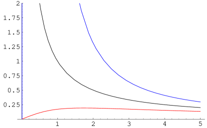
Figure 1: The potentials $U(\gamma)$ for the ESNS, the Witten BH and the ESBH.

In figure 1 the potential $U$ is plotted as function of the auxiliary dilaton $\gamma$. The lowest branch is associated with the ESBH, the one on top with the ESNS and the one in the middle with the Witten BH (i.e., the third entry in table 1). The regularity of the ESBH is evident, as well as the convergence of all three branches for $\gamma\to\infty$, encoding (T-)self-duality of the Witten BH. For small values of the dilaton the discrepancy between the ESBH, the ESNS and the Witten BH is very pronounced. Note that $U$ remains bounded globally only for the ESBH, concurring with the absence of a curvature singularity.

The two constants of motion — mass and charge — may be parameterized by $k$ and $\phi_{0}$, respectively. Thus, the level $k$ is not fixed a priori but rather emerges as a constant of motion, namely essentially the ADM mass. A rough interpretation of this — from the stringy point of view rather unexpected — result has been provided in [26] and coincides with a similar one in [63]. There is actually a physical reason why $k$ defines the mass: in the presence of matter the conservation equation $\operatorname{d}\!M=0$ (with $M$ from (10)) acquires a matter contribution, $\operatorname{d}\!M=W^{(m)}$, where $W^{(m)}=\operatorname{d}\!{\mathcal{C}}^{(m)}$ is an exact 1-form defined by the energy-momentum tensor (cf. section 5 of [4] or [66]). In a nutshell, the addition of matter deforms the total mass which now consists of a geometric and a matter part, $M$ and ${\mathcal{C}}^{(m)}$, respectively. Coming back to the ESBH, the interpretation of $k$ as mass according to the preceding discussion implies that the addition of matter should “deform” $k$. But this is precisely what happens: adding matter will in general change the central charge and hence the level $k$. Thus, from an intrinsically 2D dilaton gravity point of view the interpretation of $k$ as mass is not only possible but favored.

It could be interesting to generalize the target space action of 2D type 0A/0B, (21), as to include the non-perturbative corrections implicit in the ESBH by adding (22) (not necessarily with the choice (23)) to the ESBH action (29). However, it is not quite clear how to incorporate the term from the D0 branes — perturbatively one should just add $b^{2}q^{2}/8\pi$ to $V$ in (31), but non-perturbatively this need not be correct. More results and speculations concerning applications of the ESBH action can be found in [26].

4 Black Holes

BHs are fascinating objects, both from a theoretical and an experimental point of view [67]. Many of the features which are generic for BHs are already exhibited by the simplest members of this species, the Schwarzschild and Reissner-Nordström BHs (sometimes the Schwarzschild BH even is dubbed as “Hydrogen atom of General Relativity”). Since both of them, after integrating out the angular part, belong to the class of 2D dilaton gravity models (the first and twelfth model in table 1), the study of (3) at the classical, semi-classical and quantum level is of considerable importance for the physics of BHs.

4.1 Classical analysis

In section 2.2 it has been recalled briefly how to obtain all classical solutions in basic EF patches, (11). By looking at the geodesics of test particles and completeness properties it is straightforward to construct all Carter-Penrose diagrams for a generic model (3) (or, equivalently, (1)). For a detailed description of this algorithm cf. [34, 33, 4] and references therein.

4.2 Thermodynamics

Mass

The question of how to define “the” mass in theories of gravity is notoriously cumbersome. A nice clarification for ${\rm D}=4$ is contained in [68]. The main conceptual point is that any mass definition is meaningless without specifying 1. the ground state space-time with respect to which mass is being measured and 2. the physical scale in which mass units are being measured. Especially the first point is emphasized here. In addition to being relevant on its own, a proper mass definition is a pivotal ingredient for any thermodynamical study of BHs. Obviously, any mass-to-temperature relation is meaningless without defining the former (and the latter). For a large class of 2D dilaton gravities these issues have been resolved in [69]. One of the key ingredients is the existence [70, 71] of a conserved quantity (10) which has a deeper explanation in the context of first order gravity [72] and Poisson-sigma models [31]. It establishes the necessary prerequisite for all mass definitions, but by itself it does not yet constitute one. Ground state and scale still have to be defined. Actually, one can take $M$ from (10) provided the two ambiguities from integration constants in (4) are fixed appropriately. This is described in detail in appendix A of [51]. In those cases where this notion makes sense $M$ then coincides with the ADM mass.

Hawking temperature

There are many ways to calculate the Hawking temperature, some of them involving the coupling to matter fields, some of them being purely geometrical. Because of its simplicity we will restrict ourselves to a calculation of the geometric Hawking temperature as derived from surface gravity (cf. e.g. [73]). If defined in this way it turns out to be independent of the conformal frame. However, it should be noted that identifying Hawking temperature with surface gravity is somewhat naive for space-times which are not asymptotically flat. But the difference is just a redshift factor and for quantities like entropy or specific heat actually (34) is the relevant quantity as it coincides with the period of Euclidean time (cf. e.g. [74]). Surface gravity can be calculated by taking the normal derivative $\operatorname{d}\!/\operatorname{d}\!X$ of the Killing norm (cf. (11)) evaluated on one of the Killing horizons $X=X_{h}$, where $X_{h}$ is a solution of (12), thus yielding

$$T_{H}=\frac{1}{2\pi}\Big{|}w^{\prime}(X)\Big{|}_{X=X_{h}}\,.$$ (34)

The numerical prefactor in (34) can be changed e.g. by a redefinition of the Boltzmann constant. It has been chosen in accordance with refs. [75, 4].

Entropy

In 2D dilaton gravity there are various ways to calculate the Bekenstein-Hawking entropy. Using two different methods (simple thermodynamical considerations, i.e., $\operatorname{d}\!M=T\operatorname{d}\!S$, and Wald’s Noether charge technique [76]) Gegenberg, Kunstatter and Louis-Martinez were able to calculate the entropy for rather generic 2D dilaton gravity [77]: entropy equals the dilaton field evaluated at the Killing horizon,

$$S=2\pi X_{h}\,.$$ (35)

There exist various ways to count the microstates by appealing to the Cardy formula [78] and to recover the result (35). However, the true nature of these microstates remains unknown in this approach, which is a challenging open problem. Many different proposals have been made [79].

Specific heat

By virtue of $C_{s}=T\operatorname{d}\!S/\operatorname{d}\!T$ the specific heat reads

$$C_{s}=2\pi\left.\frac{w^{\prime}}{w^{\prime\prime}}\right|_{X=X_{h}}=\gamma_{S}\,T_{H}\,,$$ (36)

with $\gamma_{S}=4\pi^{2}\,{\rm sign}\,{(w^{\prime}(X_{h}))}/w^{\prime\prime}(X_{h})$. Because it is determined solely by the conformally invariant combination of the potentials, $w$ as defined in (4), specific heat is independent of the conformal frame, too. On a curious sidenote it is mentioned that (36) behaves like an electron gas at low temperature with Sommerfeld constant $\gamma_{S}$ (which in the present case may have any sign). If $C_{s}$ is positive and $C_{s}T^{2}\gg 1$ one may calculate logarithmic corrections to the canonical entropy from thermal fluctuations and finds [80]

$$S_{\rm can}=2\pi X_{h}+\frac{3}{2}\,\ln{\Big{|}w^{\prime}(X_{h})\Big{|}}-\frac{1}{2}\,\ln{\Big{|}w^{\prime\prime}(X_{h})\Big{|}}+\dots\,.$$ (37)

Hawking-Page like phase transition

In their by now classic paper on thermodynamics of BHs in $AdS$, Hawking and Page found a critical temperature signalling a phase transition between a BH phase and a pure $AdS$ phase [17]. This has engendered much further research, mostly in the framework of the $AdS$/CFT correspondence (for a review cf. [81]). This transition is displayed most clearly by a change of the specific heat from positive to negative sign: for Schwarzschild-$AdS$ (cf. the thirteenth entry in table 1) the critical value of $X_{h}$ is given by $X_{h}^{c}=\ell^{2}/3$. For $X_{h}>X_{h}^{c}$ the specific heat is positive, for $X_{h}<X_{h}^{c}$ it is negative. By analogy, a similar phase transition may be expected for other models with corresponding behavior of $C_{s}$. Interesting speculations on a phase transition at the Hagedorn temperature $T_{h}=k/(2\pi)$ induced by a tachyonic instability have been presented recently in the context of 2D type 0A strings (cf. the penultimate model in table 1) by Olsson [83]. From equation (22) of that work one can check easily that indeed the specific heat (at fixed $q$), $C_{s}=(q^{2}/8)(T/T_{h})/(1-T/T_{h})$, changes sign at $T=T_{h}$.

4.3 Semi-classical analysis

After the influential CGHS paper [9] there has been a lot of semi-classical activity in 2D, most of which is summarized in [84, 75, 4]. In many applications one considers (1) coupled to a scalar field (16) with $F=\rm const.$ (minimal coupling). Technically, the crucial ingredient for 1-loop effects is the Weyl anomaly (cf. e.g. [85]) $<T^{\mu}_{\mu}>=R/(24\pi)$, which — together with the semi-classical conservation equation $\nabla_{\mu}<T^{\mu\nu}>=0$ — allows to derive the flux component of the energy momentum tensor after fixing some relevant integration constant related to the choice of vacuum (e.g. Unruh, Hartle-Hawking or Boulware). This method goes back to Christensen and Fulling [86]. For non-minimal coupling, e.g. $F\propto X$, there are some important modifications — for instance, the conservation equation no longer is valid but acquires a right hand side proportional to $F^{\prime}(X)$. The first calculation of the conformal anomaly in that case has been performed by Mukhanov, Wipf and Zelnikov [87]. It has been confirmed and extended e.g. in [88].

4.4 Long time behavior

The semi-classical analysis, while leading to interesting results, has the disadvantage of becoming unreliable as the mass of the evaporating BH drops to zero. The long time behavior of an evaporating BH presents a challenge to theoretical physics and touches relevant conceptual issues of quantum gravity, such as the information paradox. There are basically two strategies: top-down, i.e., to construct first a full quantum theory of gravity and to discuss BH evaporation as a particular application thereof, and bottom-up, i.e., to sidestep the difficulties inherent to the former approach by invoking “reasonable” ad-hoc assumptions. The latter route has been pursued in [12]. A crucial technical ingredient has been Izawa’s result [89] on consistent deformations of 2D BF theory, while the most relevant physical assumption has been boundedness of the asymptotic matter flux during the whole evaporation process. Together with technical assumptions which can be relaxed, the dynamics of the evaporating BH has been described by means of consistent deformations of the underlying gauge symmetries with only one important deformation parameter. In this manner an attractor solution, the endpoint of the evaporation process, has been found (cf. the eighth model in table 1).

Ideologically, this resembles the exact renormalization group approach, cf. e.g. [90, 91] and references therein, which is based upon Weinberg’s idea of “asymptotic safety”. There are, however, several conceptual and technical differences, especially regarding the truncation of “theory space”: in 4D a truncation to EH plus cosmological constant, undoubtedly a very convenient simplification, may appear to be somewhat ad-hoc, whereas in 2D a truncation to (3) comprises not only infinitely many different theories, but essentially all theories with the same field content as (3) and the same kind of local symmetries (Lorentz transformations and diffeomorphisms).

The global structure of an evaporating BH can also be studied, and despite of the differences between various approaches there seems to be partial agreement on it, cf. e.g. [93, 94, 12, 95, 96, 91]. The crucial insight might be that a BH in the mathematical sense (i.e., an event horizon) actually never forms, but only some trapped region, cf. figure 5 in [96].

4.5 Killing horizons kill horizon degrees

As pointed out by Carlip [97], the fact that very different approaches to explain the entropy of BHs nevertheless agree on the result urgently asks for some deeper explanation. Carlip’s suggestion was to consider an underlying symmetry, somehow attached to the BH horizon, as the key ingredient, and he noted that requiring the presence of a horizon imposes constraints on the physical phase space. Actually, the change of the phase-space structure due to a constraint which imposes the existence of a horizon in space-time is an issue which is of considerable interest by itself.

In a recent work [98] we could show that the classical physical phase space is smaller as compared to the generic case if horizon constraints are imposed. Conversely, the number of gauge symmetries is larger for the horizon scenario. In agreement with a conjecture by ’t Hooft [99], we found that physical degrees of freedom are converted into gauge degrees of freedom at a horizon. We will now sketch the derivation of this result briefly for the action (3) which differs from the one used in [98] by a (Gibbons-Hawking) boundary term. For sake of concreteness we will suppose the boundary is located at $x^{1}=\rm const$. Consistency of the variational principle then requires

$$X^{+}\delta e_{0}^{-}+X^{-}\delta e_{0}^{+}+X\delta\omega_{0}=0$$ (38)

at the boundary. Note that one has to fix the parallel component of the spin-connection at the boundary rather than the dilaton field, which is the main difference to [98]. The generic case imposes $\delta e_{0}^{\pm}=0=\delta\omega_{0}$, while a horizon allows the alternative prescription $\delta e_{0}^{-}=X^{-}=0=\delta\omega_{0}$. One can now proceed in the same way as in [98], i.e., derive the constraints (the only boundary terms in the secondary constraints are now $X$ and $X^{\pm}$, while the primary ones have none) and calculate the constraint algebra. All primary constraints and the Lorentz constraint turn out to be first class, even at the boundary, whereas the Poisson bracket between the two diffeomorphism constraints ($G_{2}$, $G_{3}$ in the notation of [98]) acquires a boundary term of the form

$$X(U^{\prime}X^{+}X^{-}+V^{\prime})+U(X)X^{+}X^{-}-V(X)\,.$$ (39)

Notably, it vanishes only for $V\propto X$ and $U\propto 1/X$, e.g. for the second, third and sixth model in table 1, i.e., $(A)dS_{2}$ ground state models. The boundary constraints for the generic case convert all primary constraints into second class constraints. The construction of the reduced phase space works in the same way as in section 6 of [98], thus establishing again one physical degree of freedom “living on the boundary”. Actually, this had been known already before [100]. The horizon constraints, however, lead to more residual gauge symmetries and to a stronger fixing of free functions — in fact, no free function remains and the reduced phase space is empty. Thus, the physical degree of freedom living on a generic boundary is killed by a Killing horizon.

It would be interesting to generalize this physics-to-gauge conversion at a horizon to the case with matter. Obviously, it will no longer be a Killing horizon, but one can still employ the (trapping) horizon condition $X^{-}=0$.

4.6 Critical collapse

Critical phenomena in gravitational collapse have been discovered in the pioneering numerical investigations of Choptuik [101]. He studied a free massless scalar field coupled to spherically symmetric EH gravity in 4D (the EMKG) with sophisticated numerical techniques that allowed him to analyze the transition in the space of initial data between dispersion to infinity and the formation of a BH. Thereby the famous scaling law

$$M_{BH}\propto(p-p_{\ast})^{\gamma}\,,$$ (40)

has been established, where $p\in[0,1]$ is a free parameter characterizing a one-parameter family of initial data with the property that for $p<p_{\ast}$ a BH never forms while for $p>p_{\ast}$ a BH always forms with mass $M_{BH}$ determined by (40) for $p$ sufficiently close to $p_{\ast}$. The critical parameter $p_{\ast}\in(0,1)$ may be found by elaborate numerical analysis and depends on the specific family under consideration; but the critical exponent $\gamma\approx 0.37$ is universal, albeit model dependent. Other systems may display a different critical behavior, cf. the review [102]. The critical solution $p=p_{\ast}$, called the “Choptuon”, in general exhibits remarkable features, e.g. discrete or continuous self-similarity and a naked singularity.

Since the original system studied by Choptuik, (20), is a special case of (1) (with $U,V$ as given by the first line in table 1) coupled to (16), it is natural to inquire about generalizations of critical phenomena to arbitrary 2D dilaton gravity with scalar matter. Indeed, in [103] a critical exponent $\gamma=1/2$ has been derived analytically for the RST model [104], a semi-classical generalization of the CGHS model (cf. the third line in table 1). Later, in [105] critical collapse within the CGHS model has been considered and $\gamma\approx 1/2$ has been found numerically. More recently the generalization of the original Choptuik system to D dimensions has been considered [106, 107, 108]. For $3.5\leq D\leq 14$ the approximation $\gamma(D)\approx 0.47(1-\exp{(-0.41D)})$ shows that $\gamma$ increases monotonically with D. Since formally the CGHS corresponds to the limit ${\rm D}\to\infty$ one may expect that $\gamma(D)$ asymptotes to the value $\gamma\approx 1/2$.

In the remainder of this subsection we will establish evolution equations for generic 2D dilaton gravity with scalar matter, to be implemented numerically analogously to [109, 110]. In these works for various reasons Sachs-Bondi gauge has been used. Thus we employ

$$e_{0}^{+}=0\,,\quad e_{0}^{-}=1\,,\quad x^{0}=X\,,$$ (41)

while the remaining Zweibein components are parameterized as

$$e_{1}^{-}=\alpha(u,X)\,,\quad e_{1}^{+}=I(X)e^{2\beta(u,X)}\,.$$ (42)

In the gauge (41) with the parameterization (42) the line element reads

$$\operatorname{d}\!s^{2}=2I(X)e^{2\beta(u,X)}\operatorname{d}\!u\left(\operatorname{d}\!X+\alpha(u,X)\operatorname{d}\!u\right)\,.$$ (43)

A trapping horizon emerges either if $\alpha=0$ or $\beta\to\infty$. The equations of motion may be reduced to the following set:

$${\rm Slicing\,\,condition:} \partial_{X}\alpha(u,X) =-e^{2\beta(u,X)}w^{\prime}(X)$$ (44)

$${\rm Hamiltonian\,\,constraint:} \partial_{X}\beta(u,X) =-F(X)(\partial_{X}{\mathcal{T}}(u,X))^{2}$$ (45)

$${\rm Klein-Gordon\,\,equation:} \square\;{\mathcal{T}}(u,X) =0$$ (46)

with

$$\square=2\partial_{X}\partial_{u}-2\partial_{X}(\alpha(u,X)\partial_{X})-\frac{F^{\prime}(X)}{F(X)}\left(2\alpha(u,X)\partial_{X}-\partial_{u}\right)\,.$$ (47)

These equations should be compared with (2.12a), (2.12b) in [109] or with (2.4) (and for the Klein-Gordon equation also (2.3)) in [110], where they have been derived for spherically symmetric EH gravity in 4D. In the present case they are valid for generic 2D dilaton gravity coupled non-minimally to a free massless scalar field. Thus, the set of equations (44)-(47) is a suitable starting point for numerical simulations in generic 2D dilaton gravity. The Misner-Sharp mass function

$$m(u,X)=-X^{+}X^{-}I(X)-w(X)=-\alpha(u,X)e^{-2\beta(u,X)}-w(X)$$ (48)

allows to rewrite the condition for a trapped surface as $\alpha e^{-2\beta}=0$ (cf. (12) with (10)). Thus, as noted before, either $\alpha$ has to vanish or $\beta\to\infty$; it is the latter type of horizon that is of relevance for numerical simulations of critical collapse. One may use the Misner-Sharp function instead of $\alpha$ and thus obtains instead of (44)

$$\partial_{X}m(u,X)=(m(u,X)+w(X))2F(X)(\partial_{X}{\mathcal{T}}(u,X))^{2}\,.$$ (49)

To monitor the emergence of a trapped surface numerically one has to check whether

$$m(u_{0},X_{h})+w(X_{h})\approx 0$$ (50)

is fulfilled to a certain accuracy at a given retarded time $u_{0}$; the quantity $X_{h}$ corresponds to the value of the dilaton field at the horizon. By analogy to (2.16) of [110] one may now introduce a compactified “radial” coordinate, e.g. $X/(1+X)$, although there may be more convenient choices.

As a consistency check the original Choptuik system in the current notation will be reproduced. We recall that (20) describes the EMKG. Using $\operatorname{d}\!r=I(X)\operatorname{d}\!X$ the evolution equations for geometry read:

$$\partial_{r}\beta=\frac{\kappa}{2}r(\partial_{r}{\mathcal{T}})^{2}$$ (51)

$$\partial_{r}\alpha=\lambda^{2}e^{2\beta}$$ (52)

They look almost the same as (2.4) in [110]. The coupling constant $\kappa$ just has to be fixed appropriately in (51) (i.e. $\kappa=4\pi$). Also, the scaling constant $\lambda$ must be fixed. Note that the line element reads

$$\operatorname{d}\!s^{2}=2\frac{2}{r}e^{2\beta(u,X(r))}\operatorname{d}\!u\left(\operatorname{d}\!r\frac{r}{2}+\alpha(u,X(r))\operatorname{d}\!u\right)=2e^{2\beta}\operatorname{d}\!u\left(\operatorname{d}\!r+\frac{2\alpha}{r}\operatorname{d}\!u\right)$$ (53)

This shows that $\beta$ here really coincides with $\beta$ in [110] and $\alpha$ here coincides, up to a numerical factor, with $V$ there (and there are some signs due to different conventions).

4.7 Quasinormal modes

The term “quasinormal modes” refers to some set of modes with a complex frequency, associated with small perturbations of a BH. For $U=0$ and monomial $V$ in [111] quasinormal modes arising from a scalar field, (16) with $f=0$ and $F\propto X^{p}$, have been studied in the limit of high damping by virtue of the “monodromy approach”, and the relation

$$e^{\omega/T_{H}}=-(1+2\cos{(\pi(1-p))})$$ (54)

for the frequency $\omega$ has been found ($T_{H}$ is Hawking temperature as defined in (34)). Minimally coupled scalar fields ($p=0$) lead to the trivial result $\omega/T_{H}=2\pi in$. High damping implies that the integer $n$ has to be large. For the important case of $p=1$ (relevant for the first and fifth entry in table 1) one obtains from (54)

$$\frac{\omega}{T_{H}}=2\pi i\left(n+\frac{1}{2}\right)+\ln{3}\,.$$ (55)

The result (55) coincides with the one obtained for the Schwarzschild BH with 4D methods, both numerically [112] and analytically [113]. Moreover, consistency with ${\rm D}>4$ is found as well [114]. This shows that the 2D description of BHs is reliable also with respect to highly damped quasinormal modes.

4.8 Solid state analogues

BH analogues in condensed matter systems go back to the seminal paper by Unruh [115]. Due to the amazing progress in experimental condensed matter physics, in particular Bose-Einstein condensates, in the past decade the subject of BH analogues has flourished, cf. e.g. [116] and references therein.

In some cases the problem effectively reduces to 2D. It is thus perhaps not surprising that an analogue system for the Jackiw-Teitelboim model has been found [117] for a cigar shaped Bose-Einstein condensate. More recently this has led to some analogue 2D activity [118]. Note, however, that some issues, like the one of backreaction, might not be modelled very well by an effective action method [119]. Indeed, 2D dilaton gravity with matter could be of interest in this context, because these systems might allow not just kinematical but dynamical equivalence, i.e., not only the fluctuations (e.g. phonons) behave as the corresponding gravitational ones (e.g. Hawking quanta), but also the background dynamics does (e.g. the flow of the fluid or the metric, respectively). Such a system would be a necessary pre-requisite to study issues of mass and entropy in an analogue context. At least for static solutions this is possible [120], but of course the non-static case would be much more interesting. Alas, it is not only more interesting but also considerably more difficult, and a priori there is no reason why one should succeed in finding a fully fledged analogue model of 2D dilaton gravity with matter. Still, one can hope and try.

5 Geometry from matter

In first order gravity (3) coupled to scalar (16) or fermionic (17) matter the geometry can be quantized exactly: after analyzing the constraints, fixing EF gauge

$$(\omega_{0},e_{0}^{-},e_{0}^{+})=(0,1,0)$$ (56)

and constructing a BRST invariant Hamiltonian, the path integral can be evaluated exactly and a (nonlocal) effective action is obtained [121]. Subsequently the matter fields can be quantized by means of ordinary perturbation theory. To each order all backreactions are included automatically by this procedure.

Figure 2: VBH

Although geometry has been integrated out exactly, it can be recovered off-shell in the form of interaction vertices of the matter fields, some of which resemble virtual black holes (VBHs) [122, 123, 15]. This metamorphosis of geometry however does not take place in the matterless case [124], where the quantum effective action coincides with the classical action in EF gauge. We hasten to add that one should not take this off-shell geometry at face value — this would be like over-interpreting the role of virtual particles in a loop diagram. But the simplicity of such geometries and the fact that all possible configurations are summed over are both nice qualitative features of this picture.

A Carter-Penrose diagram of a typical VBH configuration is depicted in figure 2. The curvature scalar of such effective geometries is discontinuous and even has a $\delta$-peak. A typical effective line element (for the EMKG) reads

$$(\operatorname{d}\!s)^{2}=2\operatorname{d}\!r\operatorname{d}\!u+\left(1-\theta(r_{y}-r)\delta(u-u_{y})\left(\frac{2m}{r}+ar-d\right)\right)(\operatorname{d}\!u)^{2}\,,$$ (57)

It obviously has a Schwarzschild part with $r_{y}$-dependent “mass” $m$ and a Rindler part with $r_{y}$-dependent “acceleration” $a$, both localized on a lightlike cut. This geometry is nonlocal in the sense that it depends not just on the coordinates $r,u$ but additionally on a second point $r_{y},u_{y}$. While the off-shell geometry (57) is highly gauge dependent, the ensuing S-matrix — the only physical observable in this context [125] — appears to be gauge independent, although a formal proof of this statement, e.g. analogously to [126], is lacking.

5.1 Scalar matter

After integrating out geometry and the ghost sector (for $f(X,{\mathcal{T}})=0$), the effective Lagrangian ($w$ is defined in (4))

$${\cal L}^{\rm eff}_{\mathcal{T}}=F(\hat{X})(\partial_{0}{\mathcal{T}})(\partial_{1}{\mathcal{T}})-w^{\prime}(\hat{X})+\rm sources$$ (58)

contains the quantum version of the dilaton field $\hat{X}=\hat{X}(\nabla_{0}^{-2}(\partial_{0}{\mathcal{T}})^{2})$, depending non-locally on ${\mathcal{T}}$. The quantity $\hat{X}$ solves the equation of motion of the classical dilaton field, with matter terms and external sources for the geometric variables in EF gauge. The simplicity of (58) is in part due to the gauge choice (56) and in part due to the linearity of the gauge fixed Lagrangian in the remaining gauge field components, thus producing delta-functionals upon path integration.

In principle, the interaction vertices can be extracted by expanding the nonlocal effective action in a power series of the scalar field ${\mathcal{T}}$. However, this becomes cumbersome already at the ${\mathcal{T}}^{4}$ level. Fortunately, the localization technique introduced in [121] simplifies the calculations considerably. It relies on two observations: First, instead of dealing with complicated nonlocal kernels one may solve corresponding differential equations after imposing asymptotic conditions on the solutions. Second, instead of taking the $n$-th functional derivative of the action with respect to bilinear combinations of ${\mathcal{T}}$, the matter fields may be localized at $n$ different space-time points, which mimics the effect of functional differentiation. For tree-level calculations it is then sufficient to solve the classical equations of motion in the presence of these sources, which is achieved most easily via appropriate matching conditions.

It turns out (as anticipated from (57)) that the conserved quantity (10) is discontinuous for a VBH. This phenomenon is generic [15]. The corresponding Feynman diagrams are contained in figure 3.

Figure 3: Non-local 4-point vertices

For free, massless, non-minimally coupled scalars ($F\neq\rm const.$) both the symmetric and the non-symmetric 4-point vertex

$$V^{(4)}=\int\operatorname{d}\!^{2}x\operatorname{d}\!^{2}y(\partial_{0}{\mathcal{T}})^{2}_{x}\left[V_{\rm a}(x,y)(\partial_{0}{\mathcal{T}})^{2}_{y}+V_{\rm b}(x,y)(\partial_{0}{\mathcal{T}})_{y}(\partial_{1}{\mathcal{T}})_{y}\right]$$ (59)

are given in [15], and have the following properties:

1. They are local in one coordinate (e.g. containing $\delta(x^{1}-y^{1})$) and nonlocal in the other.

2. They vanish in the local limit ($x^{0}\to y^{0}$). Additionally, $V_{\rm b}$ vanishes for minimal coupling $F={\rm const.}$

3. The symmetric vertex depends only on the conformal invariant combination $w(X)$ and the asymptotic value $M_{\infty}$ of (10). The non-symmetric one is independent of $U$, $V$ and $M_{\infty}$. Thus if $M_{\infty}$ is fixed in all conformal frames, both vertices are conformally invariant.

4. They respect the ${\mathbb{Z}}_{2}$ symmetry $F(X)\mapsto-F(X)$.

It should be noted that the class of models with $UV+V^{\prime}=0$ and $F={\rm const}$ (containing the CGHS model, the seventh and eleventh entry in table 1) shows “scattering triviality”, i.e., the classical vertices vanish, and scattering can only arise from higher order quantum backreactions. For these models the VBH has no classically observable consequences, but at 1-loop level physical observables like the specific heat are modified appreciably [127].

The 2D Klein-Gordon equation relevant for the construction of asymptotic states is also conformally invariant. For minimal coupling it simplifies considerably, and a complete set of asymptotic states can be obtained explicitly. Since both, asymptotic states and vertices, only depend on $w(X)$ and $M_{\infty}$, at tree level conformal invariance holds nonperturbatively (to all orders in ${\mathcal{T}}$), but it is broken at 1-loop level due to the conformal anomaly. Because asymptotically geometry does not fluctuate, a standard Fock space may be built with creation/annihilation operators $a^{\pm}(k)$ obeying the standard commutation relations. The S-matrix for two ingoing ($q,q^{\prime}$) into two outgoing ($k,k^{\prime}$) asymptotic modes is determined by (cf. (59))

$$T(q,q^{\prime};k,k^{\prime})=\frac{1}{2}\langle 0\left|a^{-}(k)a^{-}(k^{\prime})V^{(4)}a^{+}(q)a^{+}(q^{\prime})\right|0\rangle\,.$$ (60)

The simple choice $M_{\infty}=0$ yields a “standard QFT vacuum” $|0\rangle$, provided the model under consideration has a Minkowskian ground state (e.g. the first, third, fifth and last model in table 1).

For the physically interesting case of the EMKG model such an S-matrix was obtained in [128, 123]. Both the symmetric and the non-symmetric vertex contribute, each giving a divergent contribution to the S-matrix, but the sum of both turned out to be finite! The whole calculation is highly nontrivial, involving cancellations of polylogarithmic terms, but at the end giving the surprisingly simple result

$$T(q,q^{\prime};k,k^{\prime})=-\frac{i\kappa\delta\left(k+k^{\prime}-q-q^{\prime}\right)}{2(4\pi)^{4}|kk^{\prime}qq^{\prime}|^{3/2}}E^{3}\tilde{T}\,,$$ (61)

with ingoing ($q,q^{\prime}$) and outgoing ($k,k^{\prime}$) spatial momenta, total energy $E=q+q^{\prime}$,

$$\tilde{T}:=\frac{1}{E^{3}}{\Bigg{[}}\Pi\ln{\frac{\Pi^{2}}{E^{6}}}+\frac{1}{\Pi}\sum_{p\in\left\{k,k^{\prime},q,q^{\prime}\right\}}p^{2}\ln{\frac{p^{2}}{E^{2}}}\cdot{\Bigg{(}}3kk^{\prime}qq^{\prime}-\frac{1}{2}\sum_{r\neq p}\sum_{s\neq r,p}\left(r^{2}s^{2}\right){\Bigg{)}}{\Bigg{]}},$$ (62)

and the momentum transfer function $\Pi=(k+k^{\prime})(k-q)(k^{\prime}-q)$. The factor $\tilde{T}$ is invariant under rescaling of the momenta $p\mapsto ap$, and the whole amplitude transforms monomial like $T\mapsto a^{-4}T$. It should be noted that due to the non-locality of the vertices there is just one $\delta$-function of momentum conservation (but no separate energy conservation) present in (61). This is advantageous because it eliminates the problem of “squared $\delta$-functions” that is otherwise present in 2D theories of massless scalar fields (cf. e.g. [129]). In this sense gravity acts as a regulator of the theory.

The corresponding differential cross section also reveals interesting features [123]:

1. For vanishing $\Pi$ forward scattering poles are present.

2. There is an approximate self-similarity close to the forward scattering peaks. Far away from them it is broken, however.

3. It is CPT invariant.

4. An ingoing s-wave can decay into three outgoing ones. Although this may be expected on general grounds, within the present formalism it is possible to provide explicit results for the decay rate.

Although it seems straightforward to generalize (60) to arbitrary $n$-point vertices, no such calculation has been attempted so far. This is related to the fact that the derivation of (61) has been somewhat tedious and lengthy. Thus, it could be worthwhile to find a more efficient way to obtain this interesting S-matrix element.

5.2 Fermionic matter

Recently we considered 2D dilaton gravity (3) coupled to fermions (17) along the lines of the previous subsection. The results will be published elsewhere, but we give a short summary with emphasis on differences to the scalar case.

The constraint analysis for the general case (17) has been worked out first in [42]. Three first class constraints generating the two diffeomorphisms and the local Lorentz symmetry and four well-known second class constraints relating the four real components of the Dirac spinor to their canonical momenta are present in the system. As anticipated the Hamiltonian is fully constrained. After introducing the Dirac bracket the constructions of the BRST charge and the gauge fixed Hamiltonian are straightforward. Path integration over geometry is even simpler than in the scalar case, because the second class constraints are implemented in the path integral through delta functionals, allowing to integrate out the fermion momenta. The effective Lagrangian

$${\cal L}^{\rm eff}_{\chi} = \frac{i}{\sqrt{2}}F(\hat{X})(\chi^{*}_{1}\overleftrightarrow{\partial_{1}}\chi_{1})$$ (63)

$$+I(\hat{X})\left(\frac{i}{\sqrt{2}}F(\hat{X})(\chi^{*}_{0}\overleftrightarrow{\partial_{0}}\chi_{0})+H(\hat{X})g(\overline{\chi}\chi)-V(\hat{X})\right)+\rm sources$$

again depends on the quantum version $\hat{X}=\hat{X}(\nabla_{0}^{-2}(\chi^{*}_{1}\overleftrightarrow{\partial_{0}}\chi_{1}))$ of the dilaton field and exhibits non-locality in the matter field.

Some properties remain the same as compared to previous studies with scalar matter. For instance, the VBH phenomenon is still present, now even for the eleventh model in table 1. In fact, the conserved quantity (10) now becomes continuous only for the trivial case $F(X)=0$. But there are also some notable differences. For example, the non-selfinteracting system already has three 4-point vertices, two of them being the symmetric and asymmetric vertices of the scalar case and a new third one, arising from the first term in the second line of (63). All vertices show the first two properties listed above, and the symmetric and non-symmetric ones also the third one.

The new vertex however does not vanish for minimal coupling, and thus in contrast to the scalar case there are two vertices present even for this simple case. It is not conformally invariant, but rather transforms additively because it contains a term proportional to $U(X)$. However, since also the external legs have a conformal weight, conformal invariance of the tree-level S-matrix still is expected to hold, despite of the non-invariance of some of the vertices and some of the asymptotic modes.

At 1-loop level and for minimal coupling conformal symmetry is broken and, exactly as in the case of scalar matter, the conformal anomaly can be integrated to the non-local Polyakov action [130]. This has been applied e.g. in[131]. A possible Thirring term can be reformulated using (19) and integrated by use of the chiral anomaly, giving a Wess-Zumino [132] contribution to the effective action. In this case, a path integral over the auxiliary vector potential remains, with a highly non-local self-interaction. Whether this treatment is favourable over treating the Thirring term directly as an interaction vertex has to be decided by application.

Another peculiar feature of 2D field theories is bosonization, e.g. the quantum equivalence of the Thirring model and the Sine-Gordon model, both in flat 1+1 dimensions [133]. This issue has been addressed recently on a curved background by Frolov, Kristjánsson and Thorlacius [134] to investigate the effect of pair-production on BH space times in regions of small curvature (as compared to the microscopic length scale of quantum theory). In the framework of first order gravity it may be possible to investigate the question of bosonization even outside this simple framework, since one is able to integrate out geometry non-perturbatively.

6 Mathematical issues

In the absence of matter many of the interesting features discussed in the previous three sections are absent: there is no tachyon dynamics, no Hawking radiation, no interesting semi-classical behavior, no critical collapse, no quasinormal modes, no relevant solid state analogue, no scattering processes and no reconstruction of geometry from matter. Nevertheless, some basic features remain, like the global structure of the classical solutions or the physics-to-gauge conversion mentioned in section 4.5. Mathematically, however, the absence of matter bears some attractiveness and reveals beautiful structures responsible for the classical integrability of (3). They may allow some relevant generalizations of (3), e.g. in the context of non-commutative gravity.

6.1 Remarks on the Einstein-Hilbert action in 2D

In 2D the Einstein tensor vanishes identically for any 2D metric and thus conveys no useful information. Similarly, the 2D EH action, supplemented appropriately by boundary and corner terms, just counts the number of holes of a compact Riemannian manifold, cf. e.g. [135]. Thus, as compared to (1) or (3) the study of “pure” 2D gravity, i.e., without coupling to a dilaton field, is of rather limited interest. If one adds a cosmological constant term one may study quantum gravity in 2D by means of dynamical triangulations, cf. e.g. [136] and references therein. The EH part of the action plays no essential role, however.

It is possible to consider EH gravity in $2+\varepsilon$ dimensions, an idea which seems to go back to [137]. After taking the limit $\varepsilon\to 0$ in a specific way [138] one obtains again a dilaton gravity model (1) with $V=0$ and $U=\rm const.$ (cf. the eleventh model in table 1). That such a limit can be very subtle has been shown recently by Jackiw [139] in the context of Weyl invariant scalar field dynamics: if one simply drops the EH term in equation (3.5) of that work the Liouville model is obtained (cf. the tenth model in table 1), but Weyl invariance is lost.

6.2 Relations to 3D: Chern-Simons and BTZ

The gravitational Chern-Simons term [140] and the 3D BTZ BH [141] have inspired a lot of further research. Here we will focus on relations to (1) and (3): dimensional reduction of the BTZ to 2D has been performed in [19], cf. the fifteenth model in table 1. A reduction of the gravitational Chern-Simons term from 3D to 2D has been performed in [20], cf. the sixteenth model in table 1. Recently [142], such reductions have been exploited to calculate the entropy of a BTZ BH in the presence of gravitational Chern-Simons terms, something which is difficult to achieve in 3D because there is no manifestly covariant formulation of the Chern-Simons term, whereas the reduced theory is manifestly covariant. It is not unlikely that also other open problems of 3D gravity may be tackled with 2D methods.

6.3 Integrable systems, Poisson-sigma models and KdV surfaces

Some of the pioneering work has been mentioned already in section 2.1 and in table 1. In two seminal papers by Kummer and Schwarz [143] the usefulness of light-cone gauge for the Lorentz frame and EF gauge for the curved metric has been demonstrated for the fourteenth model in table 1, which is a rather generic one as it has non-vanishing $U$ and non-monomial $V$. A Hamiltonian analysis [72] revealed an interesting (W-)algebraic structure of the secondary constraints together with the fields $X,X^{\pm}$ as generators. The center of this algebra consists of the conserved quantity (10) and its first derivative, $\partial_{1}M$ (which, of course, vanishes on the surface of constraints). Consequently, it has been shown by Schaller and Strobl [31] that (3) is a special case of a Poisson-sigma model,

$$S_{\rm PSM}=-\int_{\mathcal{M}}\left[X^{I}\operatorname{d}\!A_{I}-\frac{1}{2}P^{IJ}A_{J}\wedge A_{I}\right]\,,$$ (64)

with a 3D target space, the coordinates of which are $X^{I}=\{X,X^{+},X^{-}\}$. The gauge fields comprise the Cartan variables, $A_{I}=\{\omega,e^{-},e^{+}\}$. Because the dimension of the Poisson manifold is odd the Poisson tensor ($I,J\in\{X,\pm\}$)

$$P^{X\pm}=\pm X^{\pm}\,,\qquad P^{+-}=X^{+}X^{-}U(X)+V(X)\,,\qquad P^{IJ}=-P^{JI}\,,$$ (65)

cannot have full rank. Therefore, always a Casimir function, (10), exists, which may be interpreted as “mass”. Note that (65) indeed fulfills the required Jacobi-identities, $P^{IL}\partial_{L}P^{JK}+\mbox{\it perm}\left(IJK\right)=0$. For a generic (graded) Poisson-sigma model (64) the commutator of two symmetry transformations

$$\delta X^{I} =P^{IJ}\varepsilon_{J}\ , \delta A_{I} =-\operatorname{d}\!\varepsilon_{I}-\left(\partial_{I}P^{JK}\right)\varepsilon_{K}\,A_{J}\ ,$$ (66)

is a (non-linear) symmetry modulo the equations of motion. Only for $P^{IJ}$ linear in $X^{I}$ a Lie algebra is obtained; cf. the second model in table 1. For (65) the symmetries (66) on-shell correspond to local Lorentz transformations and diffeomorphisms. Generalizations discussed in section 2.4 are particularly transparent in this approach; essentially, one has to add more target space coordinates to the Poisson manifold, some of which will be fermionic in supergravity extensions, cf. e.g. [39].

Actually, there exist various approaches to integrability of gravity models in 2D, cf. e.g. [145], and we can hardly do them justice here. We will just point out a relation to Korteweg-de Vries (KdV) surfaces as discussed recently in [146]. These are 2D surfaces embedded in 3D Minkowski space arising from the KdV equation $\partial_{t}w=\partial_{x}^{3}w+6w\partial_{x}w$, with line element (cf. (11) in [146]; $u$ there coincides with $w$ here) $\operatorname{d}\!s^{2}=2\operatorname{d}\!X\operatorname{d}\!u-(4\lambda-w(X,u))\operatorname{d}\!u^{2}$, where $X\propto x$, $u\propto t$ and $\lambda$ is some constant. For static KdV solutions, $\partial_{u}w=0$, this line element is also a solution of (3) as can bee seen from (11), with $\lambda$ playing the role of the mass $M$. In the non-static case it describes a solution of (3) coupled to some energy-momentum tensor. It could be of interest to pursue this relation in more depth.

6.4 Torsion and non-metricity

For $U=0$ the equation of motion $R=2V^{\prime}(X)$, if invertible, allows to rewrite the action (1) as $S_{\rm R}=\int\operatorname{d}\!^{2}x\sqrt{-g}f(R)$, cf. e.g. [147] and references therein. As compared to such theories, the literature on models with torsion $\tau^{a}={\ast T^{a}}$,

$$S_{\rm RT}=\int\operatorname{d}\!^{2}x\sqrt{-g}f(R,\tau^{a}\tau_{a})\,,$$ (67)

is relatively scarce and consists mainly of elaborations based upon the fourteenth model in table 1, where $f=A\tau^{a}\tau_{a}+BR^{2}+CR+\Lambda$, also known as “Poincarè gauge theory”, cf. [148] and references therein. This model in particular (and a large class of models of type (67)) allows an equivalent reformulation as (3). Thus, they need not be discussed separately.

A generalization which includes also effects from non-metricity has been studied in [149]. Elimination of non-metricity leads again to models of type (1), (3), but one has to be careful with such reformulations as test-particles moving along geodesics or, alternatively, along auto-parallels, may “feel” the difference. Thus, it could be of interest to generalize (3) (which already contains torsion if $U\neq 0$) as to include non-metricity, thus dropping the requirement that the connection $\omega^{a}{}_{b}$ is proportional to $\varepsilon^{a}{}_{b}$. However, a formulation as Poisson-sigma model (64) (with 6D target space) seems to be impossible as there are only trivial solutions to the Jacobi identities.

6.5 Non-commutative gravity

In the 1970ies/1980ies theories have been supersymmetrized, in the 1990ies/2000s theories have been “non-commutativized”, for reviews cf. e.g. [150]. The latter procedure still has not stopped as the original idea, namely to obtain a fully satisfactory non-commutative version of gravity, has not been achieved so far. In order to get around the main conceptual obstacles it is tempting to consider the simplified framework of 2D.

There it is possible to construct non-commutative dilaton gravity models with a usual (non-twisted) realization of gauge symmetries. A non-commutative version of the Jackiw-Teitelboim model (cf. the second entry in table 1),

$$S_{\rm NCJT}=-\frac{1}{2}\int d^{2}x\,\varepsilon^{\mu\nu}\left[X_{a}\star T_{\mu\nu}^{a}+X_{ab}\star\left(R_{\mu\nu}^{ab}-\Lambda e_{\mu}^{a}\star e_{\nu}^{b}\right)\right]\,,$$ (68)

has been constructed in [152] and then quantized in [153]. A non-commutative version of the fourth model in table 1 was suggested in [154]. For a definition of the Moyal-$\star$ and further notation cf. these two references. A crucial change as compared to (3), besides the $\star$, is the appearance of a second dilaton field $\psi$ in $2X_{ab}=X\varepsilon_{ab}-i\psi\eta_{ab}$. However, interesting as these results may be, there seems to be no way to generalize them to generic 2D dilaton gravity without twisting the gauge symmetries [155]. Moreover, the fact that the metric can be changed by “Lorentz transformations” seems questionable from a physical point of view, cf. [156] for a similar problem.

An important step towards constructing a satisfactory non-commutative gravity was recently made by Wess and collaborators [157], who understood how one can construct diffeomorphism invariants, including the EH action, on non-commutative spaces (see also [158] for a real formulation). There is, however, a price to pay. The diffeomorphism group becomes twisted, i.e., there is a non-trivial coproduct [159]. Recently it could be shown [160] that twisted gauge symmetries close for arbitrary gauge groups and thus a construction of twisted-invariant actions is straightforward. The main element in that construction (cf. also [159, 161, 157, 158] and [162]) is the twist operator

$$\mathcal{F}=\exp\mathcal{P},\qquad\mathcal{P}=\frac{i}{2}\theta^{\mu\nu}\partial_{\mu}\otimes\partial_{\nu}\,,$$ (69)

which acts on the tensor products of functions $\phi_{1}\otimes\phi_{2}$. With the multiplication map $\mu(\phi_{1}\otimes\phi_{2})=\phi_{1}\cdot\phi_{2}$ and (69) the Moyal-Weyl representation of the star product,

$$\phi_{1}\star\phi_{2}=\mu\circ\mathcal{F}(\phi_{1}\otimes\phi_{2})=\mu_{\star}(\phi_{1}\otimes\phi_{2})\,,$$ (70)

can be constructed. Consider now generators $u$ of some symmetry transformations which form a Lie algebra. If one knows the action of these transformations on primary fields, $\delta_{u}\phi=u\phi$, the action on tensor products is defined by the coproduct $\Delta$. In the undeformed case the coproduct is primitive, $\Delta_{0}(u)=u\otimes 1+1\otimes u$ and $\delta_{u}(\phi_{1}\otimes\phi_{2})=\Delta_{0}(u)(\phi_{1}\otimes\phi_{2})=u\phi_{1}\otimes\phi_{2}+\phi_{1}\otimes u\phi_{2}$ satisfies the usual Leibniz rule. The action of symmetry generators on elementary fields is left undeformed, but the coproduct is twisted,

$$\Delta(u)=\exp(-\mathcal{P})\Delta_{0}(u)\exp(\mathcal{P})\,.$$ (71)

Obviously, twisting preserves the commutation relations. Therefore, the commutators of gauge transformations for an arbitrary gauge group close.

It seems plausible that a corresponding generalization to twisted non-linear gauge symmetries will be a crucial technical pre-requisite to a successful construction of generic non-commutative 2D dilaton gravity. It would allow, among other things, a thorough discussion of non-commutative BHs, along the lines of sections 2-5.

- [1] Such a life, with all vision limited to a Point, and all motion to a Straight Line, seemed to me inexpressibly dreary; and I was surprised to note the vivacity and cheerfulness of the King. [Edwin A. Abbot, “Flatland — A Romance of Many Dimensions.” Dover Publications 1992, New York. (first published under the pseudonym A. Square in 1884, Seeley & Co., London)].
- [2] J. Brown, Lower Dimensional Gravity. World Scientific, 1988.
- [3] A. M. Polyakov, “Quantum gravity in two-dimensions,” Mod. Phys. Lett. A2 (1987) 893.
- [4] D. Grumiller, W. Kummer, and D. V. Vassilevich, “Dilaton gravity in two dimensions,” Phys. Rept. 369 (2002) 327–429, hep-th/0204253.
- [5] P. Thomi, B. Isaak, and P. Hájíček, “Spherically symmetric systems of fields and black holes. 1. Definition and properties of apparent horizon,” Phys. Rev. D30 (1984) 1168. P. Hájíček, “Spherically symmetric systems of fields and black holes. 2. Apparent horizon in canonical formalism,” Phys. Rev. D30 (1984) 1178.
- [6] C. Teitelboim, “Gravitation and Hamiltonian structure in two space-time dimensions,” Phys. Lett. B126 (1983) 41.
- [7] R. Jackiw, “Lower dimensional gravity,” Nucl. Phys. B252 (1985) 343–356.
- [8] E. Witten, “On string theory and black holes,” Phys. Rev. D44 (1991) 314–324. G. Mandal, A. M. Sengupta, and S. R. Wadia, “Classical solutions of two-dimensional string theory,” Mod. Phys. Lett. A6 (1991) 1685–1692. S. Elitzur, A. Forge, and E. Rabinovici, “Some global aspects of string compactifications,” Nucl. Phys. B359 (1991) 581–610.
- [9] C. G. Callan, Jr., S. B. Giddings, J. A. Harvey, and A. Strominger, “Evanescent black holes,” Phys. Rev. D45 (1992) 1005–1009, hep-th/9111056.
- [10] J. P. S. Lemos and P. M. Sa, “The black holes of a general two-dimensional dilaton gravity theory,” Phys. Rev. D49 (1994) 2897–2908, arXiv:gr-qc/9311008.
- [11] A. Fabbri and J. G. Russo, “Soluble models in 2d dilaton gravity,” Phys. Rev. D53 (1996) 6995–7002, hep-th/9510109.
- [12] D. Grumiller, “Long time black hole evaporation with bounded Hawking flux,” JCAP 05 (2004) 005, gr-qc/0307005.
- [13] M. O. Katanaev, W. Kummer, and H. Liebl, “On the completeness of the black hole singularity in 2d dilaton theories,” Nucl. Phys. B486 (1997) 353–370, gr-qc/9602040.
- [14] Y. Nakayama, “Liouville field theory: A decade after the revolution,” Int. J. Mod. Phys. A19 (2004) 2771–2930, hep-th/0402009.
- [15] D. Grumiller, W. Kummer, and D. V. Vassilevich, “Virtual black holes in generalized dilaton theories (and their special role in string gravity),” European Phys. J. C30 (2003) 135–143, hep-th/0208052.
- [16] H. Reissner, “Über die Eigengravitation des elektrischen Feldes nach der Einsteinschen Theorie,” Ann. Phys. 50 (1916) 106. G. Nordström, “On the energy of the gravitation field in Einstein’s theory,” Proc. Kon. Ned. Akad. Wet. 20 (1916) 1238.
- [17] S. W. Hawking and D. N. Page, “Thermodynamics of black holes in anti-de Sitter space,” Commun. Math. Phys. 87 (1983) 577.
- [18] M. O. Katanaev and I. V. Volovich, “String model with dynamical geometry and torsion,” Phys. Lett. B175 (1986) 413–416; “Two-dimensional gravity with dynamical torsion and strings,” Ann. Phys. 197 (1990) 1.
- [19] A. Achucarro and M. E. Ortiz, “Relating black holes in two-dimensions and three- dimensions,” Phys. Rev. D48 (1993) 3600–3605, hep-th/9304068.
- [20] G. Guralnik, A. Iorio, R. Jackiw, and S. Y. Pi, “Dimensionally reduced gravitational Chern-Simons term and its kink,” Ann. Phys. 308 (2003) 222–236, hep-th/0305117.
- [21] D. Grumiller and W. Kummer, “The classical solutions of the dimensionally reduced gravitational Chern-Simons theory,” Ann. Phys. 308 (2003) 211–221, hep-th/0306036. L. Bergamin, D. Grumiller, A. Iorio, and C. Nuñez, “Chemistry of Chern-Simons supergravity: Reduction to a BPS kink, oxidation to M-theory and thermodynamical aspects,” JHEP 11 (2004) 021, hep-th/0409273.
- [22] L. Bergamin, “Constant dilaton vacua and kinks in 2d (super-)gravity,” hep-th/0509183.
- [23] M. R. Douglas et al., “A new hat for the c = 1 matrix model,” hep-th/0307195.
- [24] S. Gukov, T. Takayanagi, and N. Toumbas, “Flux backgrounds in 2D string theory,” JHEP 03 (2004) 017, hep-th/0312208.
- [25] R. Dijkgraaf, H. Verlinde, and E. Verlinde, “String propagation in a black hole geometry,” Nucl. Phys. B371 (1992) 269–314.
- [26] D. Grumiller, “An action for the exact string black hole,” JHEP 05 (2005) 028, hep-th/0501208.
- [27] K. Isler and C. A. Trugenberger, “A gauge theory of two-dimensional quantum gravity,” Phys. Rev. Lett. 63 (1989) 834. A. H. Chamseddine and D. Wyler, “Gauge theory of topological gravity in (1+1)-dimensions,” Phys. Lett. B228 (1989) 75.
- [28] H. Verlinde, “Black holes and strings in two dimensions,” in Trieste Spring School on Strings and Quantum Gravity, pp. 178–207. April, 1991. the same lectures have been given at MGVI in Japan, June, 1991.
- [29] D. Cangemi and R. Jackiw, “Gauge invariant formulations of lineal gravity,” Phys. Rev. Lett. 69 (1992) 233–236, hep-th/9203056. A. Achucarro, “Lineal gravity from planar gravity,” Phys. Rev. Lett. 70 (1993) 1037–1040, hep-th/9207108.
- [30] N. Ikeda and K. I. Izawa, “General form of dilaton gravity and nonlinear gauge theory,” Prog. Theor. Phys. 90 (1993) 237–246, hep-th/9304012.
- [31] P. Schaller and T. Strobl, “Poisson structure induced (topological) field theories,” Mod. Phys. Lett. A9 (1994) 3129–3136, hep-th/9405110.
- [32] J. G. Russo and A. A. Tseytlin, “Scalar tensor quantum gravity in two-dimensions,” Nucl. Phys. B382 (1992) 259–275, arXiv:hep-th/9201021. S. D. Odintsov and I. L. Shapiro, “One loop renormalization of two-dimensional induced quantum gravity,” Phys. Lett. B263 (1991) 183–189. T. Banks and M. O’Loughlin, “Two-dimensional quantum gravity in Minkowski space,” Nucl. Phys. B362 (1991) 649–664. R. B. Mann, A. Shiekh, and L. Tarasov, “Classical and quantum properties of two-dimensional black holes,” Nucl. Phys. B341 (1990) 134–154.
- [33] T. Klösch and T. Strobl, “Classical and quantum gravity in 1+1 dimensions. Part II: The universal coverings,” Class. Quant. Grav. 13 (1996) 2395–2422, arXiv:gr-qc/9511081.
- [34] T. Klösch and T. Strobl, “Classical and quantum gravity in (1+1)-dimensions. Part I: A unifying approach,” Class. Quant. Grav. 13 (1996) 965–984, arXiv:gr-qc/9508020.
- [35] J.-G. Hao and X.-Z. Li, “Constructing dark energy models with late time de Sitter attractor,” Phys. Rev. D68 (2003) 083514, hep-th/0306033.
- [36] L. Bergamin, D. Grumiller, and W. Kummer, “Supersymmetric black holes in 2d dilaton supergravity: baldness and extremality,” J. Phys. A37 (2004) 3881–3901, hep-th/0310006.
- [37] D. M. Thompson, “AdS solutions of 2D type 0A,” Phys. Rev. D70 (2004) 106001, hep-th/0312156.
- [38] D. Birmingham, M. Blau, M. Rakowski, and G. Thompson, “Topological field theory,” Phys. Rept. 209 (1991) 129–340.
- [39] T. Strobl, “Gravity in two spacetime dimensions,” hep-th/0011240. Habilitation thesis.
- [40] Y.-C. Park and A. Strominger, “Supersymmetry and positive energy in classical and quantum two-dimensional dilaton gravity,” Phys. Rev. D47 (1993) 1569–1575, arXiv:hep-th/9210017. J. M. Izquierdo, “Free differential algebras and generic 2d dilatonic (super)gravities,” Phys. Rev. D59 (1999) 084017, arXiv:hep-th/9807007. T. Strobl, “Target-superspace in 2d dilatonic supergravity,” Phys. Lett. B460 (1999) 87–93, arXiv:hep-th/9906230. M. Ertl, W. Kummer, and T. Strobl, “General two-dimensional supergravity from Poisson superalgebras,” JHEP 01 (2001) 042, arXiv:hep-th/0012219. M. Ertl, Supergravity in two spacetime dimensions. PhD thesis, Technische Universität Wien, 2001. arXiv:hep-th/0102140. L. Bergamin and W. Kummer, “The complete solution of 2D superfield supergravity from graded Poisson-Sigma models and the super pointparticle,” Phys. Rev. D68 (2003) 104005, hep-th/0306217; “Two-dimensional N=(2,2) dilaton supergravity from graded Poisson-Sigma models I: Complete actions and their symmetries.,” Eur. Phys. J. C39 (2005) S41–S52, hep-th/0402138; “Two-dimensional N = (2,2) dilaton supergravity from graded Poisson-Sigma models. II: Analytic solution and BPS states,” Eur. Phys. J. C39 (2005) S53–S63, hep-th/0411204. L. Bergamin, D. Grumiller, and W. Kummer, “Quantization of 2d dilaton supergravity with matter,” JHEP 05 (2004) 060, hep-th/0404004.
- [41] L. Bergamin and W. Kummer, “Graded Poisson sigma models and dilaton-deformed 2d supergravity algebra,” JHEP 05 (2003) 074, hep-th/0209209.
- [42] R. Meyer, “Constraints in two-dimensional dilaton gravity with fermions,” hep-th/0512267.
- [43] W. E. Thirring, “A soluble relativistic field theory,” Annals Phys. 3 (1958) 91–112.
- [44] H. Balasin, C. G. Boehmer, and D. Grumiller, “The spherically symmetric standard model with gravity,” Gen. Rel. Grav. 37 (2005) 1435–1482, gr-qc/0412098.
- [45] W. Kummer, “Deformed ISO(2,1) symmetry and non-Einsteinian 2d-gravity with matter,” in HADRON STRUCTURE ’92, D. Bruncko and J. Urban, eds. September, 1992. Stara Lesna, Czechoslovakia.
- [46] H. Pelzer and T. Strobl, “Generalized 2d dilaton gravity with matter fields,” Class. Quant. Grav. 15 (1998) 3803–3825, arXiv:gr-qc/9805059.
- [47] P. C. Aichelburg and R. U. Sexl, “On the gravitational field of a massless particle,” Gen. Rel. Grav. 2 (1971) 303–312.
- [48] H. Balasin and D. Grumiller, “The ultrarelativistic limit of 2d dilaton gravity and its energy momentum tensor,” Class. Quant. Grav. 21 (2004) 2859–2872, gr-qc/0312086.
- [49] I. Z. Fisher, “Scalar mesostatic field with regard for gravitational effects,” Zh. Eksp. Teor. Fiz. 18 (1948) 636–640, gr-qc/9911008.
- [50] A. T. Filippov and D. Maison, “Horizons in 1+1 dimensional dilaton gravity coupled to matter,” Class. Quant. Grav. 20 (2003) 1779–1786, gr-qc/0210081.
- [51] D. Grumiller and D. Mayerhofer, “On static solutions in 2d dilaton gravity with scalar matter,” Class. Quant. Grav. 21 (2004) 5893–5914, gr-qc/0404013.
- [52] M. Wyman, “Static spherically symmetric scalar fields in general relativity,” Phys. Rev. D24 (1981) 839–841.
- [53] A. H. Bilge and D. Daghan, “Partial decoupling and exact static solutions for Choptuik’s spacetime,” gr-qc/0508020.
- [54] M. D. Roberts, “Scalar field counterexamples to the cosmic censorship hypothesis,” Gen. Rel. Grav. 21 (1989) 907–939.
- [55] T. Takayanagi and N. Toumbas, “A matrix model dual of type 0B string theory in two dimensions,” JHEP 07 (2003) 064, hep-th/0307083.
- [56] P. Ginsparg and G. W. Moore, “Lectures on 2-d gravity and 2-d string theory,” hep-th/9304011. P. Di Francesco, P. H. Ginsparg, and J. Zinn-Justin, “2-D Gravity and random matrices,” Phys. Rept. 254 (1995) 1–133, hep-th/9306153. S. Alexandrov, “Matrix quantum mechanics and two-dimensional string theory in non-trivial backgrounds,” hep-th/0311273.
- [57] V. Kazakov, I. K. Kostov, and D. Kutasov, “A matrix model for the two-dimensional black hole,” Nucl. Phys. B622 (2002) 141–188, hep-th/0101011.
- [58] L. Bergamin, D. Grumiller, W. Kummer, and D. V. Vassilevich, “Classical and quantum integrability of 2D dilaton gravities in Euclidean space,” Class. Quant. Grav. 22 (2005) 1361–1382, hep-th/0412007.
- [59] I. R. Klebanov and A. A. Tseytlin, “D-branes and dual gauge theories in type 0 strings,” Nucl. Phys. B546 (1999) 155–181, hep-th/9811035. A. Strominger, “A matrix model for AdS(2),” JHEP 03 (2004) 066, hep-th/0312194. J. L. Davis, L. A. Pando Zayas, and D. Vaman, “On black hole thermodynamics of 2-D type 0A,” JHEP 03 (2004) 007, hep-th/0402152. U. H. Danielsson, J. P. Gregory, M. E. Olsson, P. Rajan, and M. Vonk, “Type 0A 2D black hole thermodynamics and the deformed matrix model,” JHEP 04 (2004) 065, hep-th/0402192. J. L. Davis and R. McNees, “Boundary counterterms and the thermodynamics of 2-D black holes,” JHEP 09 (2005) 072, hep-th/0411121.
- [60] A. A. Tseytlin, “On the form of the black hole solution in d = 2 theory,” Phys. Lett. B268 (1991) 175–178. I. Jack, D. R. T. Jones, and J. Panvel, “Exact bosonic and supersymmetric string black hole solutions,” Nucl. Phys. B393 (1993) 95–110, hep-th/9201039.
- [61] A. A. Tseytlin, “Effective action of gauged WZW model and exact string solutions,” Nucl. Phys. B399 (1993) 601–622, hep-th/9301015. I. Bars and K. Sfetsos, “Exact effective action and space-time geometry in gauged WZW models,” Phys. Rev. D48 (1993) 844–852, hep-th/9301047.
- [62] K. Becker, “Strings, black holes and conformal field theory,” hep-th/9404157.
- [63] V. A. Kazakov and A. A. Tseytlin, “On free energy of 2-d black hole in bosonic string theory,” JHEP 06 (2001) 021, hep-th/0104138.
- [64] M. J. Perry and E. Teo, “Nonsingularity of the exact two-dimensional string black hole,” Phys. Rev. Lett. 70 (1993) 2669–2672, hep-th/9302037. P. Yi, “Nonsingular 2-D black holes and classical string backgrounds,” Phys. Rev. D48 (1993) 2777–2788, hep-th/9302070.
- [65] D. Grumiller and D. V. Vassilevich, “Non-existence of a dilaton gravity action for the exact string black hole,” JHEP 11 (2002) 018, hep-th/0210060.
- [66] W. Kummer and P. Widerin, “Conserved quasilocal quantities and general covariant theories in two-dimensions,” Phys. Rev. D52 (1995) 6965–6975, arXiv:gr-qc/9502031.
- [67] V. Frolov and I. Novikov, Black Hole Physics. Kluwer Academic Publishers, 1998.
- [68] L. D. Faddeev, “The energy problem in Einstein’s theory of gravitation,” Sov. Phys. Usp. 25 (1982) 130–142.
- [69] H. Liebl, D. V. Vassilevich, and S. Alexandrov, “Hawking radiation and masses in generalized dilaton theories,” Class. Quant. Grav. 14 (1997) 889–904, arXiv:gr-qc/9605044.
- [70] V. P. Frolov, “Two-dimensional black hole physics,” Phys. Rev. D46 (1992) 5383–5394.
- [71] R. B. Mann, “Conservation laws and 2-d black holes in dilaton gravity,” Phys. Rev. D47 (1993) 4438–4442, hep-th/9206044.
- [72] H. Grosse, W. Kummer, P. Presnajder, and D. J. Schwarz, “Novel symmetry of nonEinsteinian gravity in two- dimensions,” J. Math. Phys. 33 (1992) 3892–3900, hep-th/9205071.
- [73] R. M. Wald, “The thermodynamics of black holes,” Living Rev. Rel. 4 (2001) 6, gr-qc/9912119.
- [74] G. W. Gibbons and S. W. Hawking, eds., Euclidean quantum gravity. Singapore: World Scientific, 1993.
- [75] W. Kummer and D. V. Vassilevich, “Hawking radiation from dilaton gravity in (1+1) dimensions: A pedagogical review,” Annalen Phys. 8 (1999) 801–827, gr-qc/9907041.
- [76] R. M. Wald, “Black hole entropy is the Nöther charge,” Phys. Rev. D48 (1993) 3427–3431, gr-qc/9307038. V. Iyer and R. M. Wald, “Some properties of Nöther charge and a proposal for dynamical black hole entropy,” Phys. Rev. D50 (1994) 846–864, gr-qc/9403028.
- [77] J. Gegenberg, G. Kunstatter, and D. Louis-Martinez, “Observables for two-dimensional black holes,” Phys. Rev. D51 (1995) 1781–1786, gr-qc/9408015.
- [78] H. W. J. Bloete, J. L. Cardy, and M. P. Nightingale, “Conformal invariance, the central charge, and universal finite size amplitudes at criticality,” Phys. Rev. Lett. 56 (1986) 742–745. J. L. Cardy, “Operator content of two-dimensional conformally invariant theories,” Nucl. Phys. B270 (1986) 186–204.
- [79] A. Strominger and C. Vafa, “Microscopic Origin of the Bekenstein-Hawking Entropy,” Phys. Lett. B379 (1996) 99–104, hep-th/9601029. K. V. Krasnov, “On statistical mechanics of gravitational systems,” Gen. Rel. Grav. 30 (1998) 53–68, gr-qc/9605047. A. Ashtekar, J. Baez, A. Corichi, and K. Krasnov, “Quantum geometry and black hole entropy,” Phys. Rev. Lett. 80 (1998) 904–907, gr-qc/9710007. M. Cadoni and S. Mignemi, “Entropy of 2d black holes from counting microstates,” Phys. Rev. D59 (1999) 081501, hep-th/9810251. S. Carlip, “Black hole entropy from conformal field theory in any dimension,” Phys. Rev. Lett. 82 (1999) 2828–2831, hep-th/9812013. S. N. Solodukhin, “Conformal description of horizon’s states,” Phys. Lett. B454 (1999) 213–222, hep-th/9812056. M.-I. Park and J. H. Yee, “Comments on ’Entropy of 2D black holes from counting microstates’,” Phys. Rev. D61 (2000) 088501, hep-th/9910213. S. Carlip, “Reply to the comment by Park and Ho on ’Black hole entropy from conformal field theory in any dimension’,” Phys. Rev. Lett. 83 (1999) 5596, hep-th/9910247. M.-I. Park and J. Ho, “Comments on ’Black hole entropy from conformal field theory in any dimension’,” Phys. Rev. Lett. 83 (1999) 5595, hep-th/9910158. I. Sachs and S. N. Solodukhin, “Horizon holography,” Phys. Rev. D64 (2001) 124023, hep-th/0107173. M.-I. Park, “Hamiltonian dynamics of bounded spacetime and black hole entropy: Canonical method,” Nucl. Phys. B634 (2002) 339–369, hep-th/0111224. N. Pinamonti and L. Vanzo, “Central charges and boundary fields for two dimensional dilatonic black holes,” Phys. Rev. D69 (2004) 084012, hep-th/0312065. G. Kang, J.-I. Koga, and M.-I. Park, “Near-horizon conformal symmetry and black hole entropy in any dimension,” Phys. Rev. D70 (2004) 024005, hep-th/0402113.
- [80] D. Grumiller, “Logarithmic corrections to the entropy of the exact string black hole,” in Path Integrals from Quantum Information to Cosmology, C. Burdik, N. Navratil, and S. Posta, eds. JINR Publishing Department, Prague, June, 2005. hep-th/0506175.
- [81] O. Aharony, S. S. Gubser, J. M. Maldacena, H. Ooguri, and Y. Oz, “Large N field theories, string theory and gravity,” Phys. Rept. 323 (2000) 183–386, hep-th/9905111.
- [82] J. D. Brown, J. Creighton, and R. B. Mann, “Temperature, energy and heat capacity of asymptotically anti-de Sitter black holes,” Phys. Rev. D50 (1994) 6394–6403, gr-qc/9405007.
- [83] M. E. Olsson, “The stringy nature of the 2d type-0A black hole,” hep-th/0511106.
- [84] J. A. Harvey and A. Strominger, “Quantum aspects of black holes,” in Recent directions in particle theory: from superstrings and black holes to the standard model (TASI - 92). 1992. hep-th/9209055. A. Strominger, “Les Houches lectures on black holes,” arXiv:hep-th/9501071. Talk given at NATO Advanced Study Institute. L. Thorlacius, “Black hole evolution,” Nucl. Phys. Proc. Suppl. 41 (1995) 245–275, hep-th/9411020. S. B. Giddings, “Quantum mechanics of black holes,” Trieste HEP Cosmology (1994) 0530–574, arXiv:hep-th/9412138.
- [85] M. J. Duff, “Twenty years of the weyl anomaly,” Class. Quant. Grav. 11 (1994) 1387–1404, hep-th/9308075.
- [86] S. M. Christensen and S. A. Fulling, “Trace anomalies and the Hawking effect,” Phys. Rev. D15 (1977) 2088–2104.
- [87] V. Mukhanov, A. Wipf, and A. Zelnikov, “On 4-D Hawking radiation from effective action,” Phys. Lett. B332 (1994) 283–291, hep-th/9403018.
- [88] T. Chiba and M. Siino, “Disappearance of black hole criticality in semiclassical general relativity,” Mod. Phys. Lett. A12 (1997) 709–718. S. Ichinose, “Weyl anomaly of 2D dilaton-scalar gravity and hermiticity of system operator,” Phys. Rev. D57 (1998) 6224–6229, hep-th/9707025. W. Kummer, H. Liebl, and D. V. Vassilevich, “Hawking radiation for non-minimally coupled matter from generalized 2d black hole models,” Mod. Phys. Lett. A12 (1997) 2683–2690, hep-th/9707041.
- [89] K. I. Izawa, “On nonlinear gauge theory from a deformation theory perspective,” Prog. Theor. Phys. 103 (2000) 225–228, hep-th/9910133.
- [90] O. Lauscher and M. Reuter, “Ultraviolet fixed point and generalized flow equation of quantum gravity,” Phys. Rev. D65 (2002) 025013, hep-th/0108040.
- [91] A. Bonanno and M. Reuter, “Spacetime structure of an evaporating black hole in quantum gravity,” hep-th/0602159.
- [92] M. Niedermaier, “Dimensionally reduced gravity theories are asymptotically safe,” Nucl. Phys. B673 (2003) 131–169, hep-th/0304117.
- [93] V. P. Frolov and G. A. Vilkovisky, “Spherically symmetric collapse in quantum gravity,” Phys. Lett. B106 (1981) 307–313.
- [94] M. K. Parikh and F. Wilczek, “Global structure of evaporating black holes,” Phys. Lett. B449 (1999) 24–29, gr-qc/9807031.
- [95] A. Ashtekar and M. Bojowald, “Black hole evaporation: A paradigm,” Class. Quant. Grav. 22 (2005) 3349–3362, gr-qc/0504029.
- [96] S. A. Hayward, “Formation and evaporation of regular black holes,” Phys. Rev. Lett. 96 (2006) 031103, gr-qc/0506126.
- [97] S. Carlip, “Horizon constraints and black hole entropy,” Class. Quant. Grav. 22 (2005) 1303–1312, hep-th/0408123; “Horizon constraints and black hole entropy,” gr-qc/0508071; “Horizons, constraints, and black hole entropy,” gr-qc/0601041.
- [98] L. Bergamin, D. Grumiller, W. Kummer, and D. V. Vassilevich, “Physics-to-gauge conversion at black hole horizons,” Class. Quant. Grav. 23 (2006) 3075–3101, hep-th/0512230.
- [99] G. ’t Hooft, “Horizons,” gr-qc/0401027.
- [100] K. V. Kuchař, “Geometrodynamics of Schwarzschild black holes,” Phys. Rev. D50 (1994) 3961–3981, gr-qc/9403003.
- [101] M. W. Choptuik, “Universality and scaling in gravitational collapse of a massless scalar field,” Phys. Rev. Lett. 70 (1993) 9–12.
- [102] C. Gundlach, “Critical phenomena in gravitational collapse,” Adv. Theor. Math. Phys. 2 (1998) 1–49, arXiv:gr-qc/9712084.
- [103] A. Strominger and L. Thorlacius, “Universality and scaling at the onset of quantum black hole formation,” Phys. Rev. Lett. 72 (1994) 1584–1587, hep-th/9312017.
- [104] J. G. Russo, L. Susskind, and L. Thorlacius, “Cosmic censorship in two-dimensional gravity,” Phys. Rev. D47 (1993) 533–539, hep-th/9209012.
- [105] Y. Peleg, S. Bose, and L. Parker, “Choptuik scaling and quantum effects in 2D dilaton gravity,” Phys. Rev. D55 (1997) 4525–4528, gr-qc/9608040.
- [106] M. Birukou, V. Husain, G. Kunstatter, E. Vaz, and M. Olivier, “Spherically symmetric scalar field collapse in any dimension,” Phys. Rev. D65 (2002) 104036.
- [107] E. Sorkin and Y. Oren, “On Choptuik’s scaling in higher dimensions,” Phys. Rev. D71 (2005) 124005, hep-th/0502034.
- [108] J. Bland, B. Preston, M. Becker, G. Kunstatter, and V. Husain, “Dimension dependence of the critical exponent in spherically symmetric gravitational collapse,” Class. Quant. Grav. 22 (2005) 5355–5364.
- [109] S. Husa, C. Lechner, M. Purrer, J. Thornburg, and P. C. Aichelburg, “Type II critical collapse of a self-gravitating nonlinear sigma-model,” Phys. Rev. D62 (2000) 104007, gr-qc/0002067.
- [110] M. Purrer, S. Husa, and P. C. Aichelburg, “News from critical collapse: Bondi mass, tails and quasinormal modes,” Phys. Rev. D71 (2005) 104005, gr-qc/0411078.
- [111] J. Kettner, G. Kunstatter, and A. J. M. Medved, “Quasinormal modes for single horizon black holes in generic 2-d dilaton gravity,” Class. Quant. Grav. 21 (2004) 5317–5332, gr-qc/0408042.
- [112] H.-P. Nollert, “Quasinormal modes of Schwarzschild black holes: The determination of quasinormal frequencies with very large imaginary parts,” Phys. Rev. D47 (1993) 5253–5258. N. Andersson, “On the asymptotic distribution of quasinormal-mode frequencies for Schwarzschild black holes,” Class. Quant. Grav. L10 (1993) 61–67.
- [113] L. Motl, “An analytical computation of asymptotic Schwarzschild quasinormal frequencies,” Adv. Theor. Math. Phys. 6 (2003) 1135–1162, gr-qc/0212096.
- [114] L. Motl and A. Neitzke, “Asymptotic black hole quasinormal frequencies,” Adv. Theor. Math. Phys. 7 (2003) 307–330, hep-th/0301173.
- [115] W. G. Unruh, “Experimental black hole evaporation,” Phys. Rev. Lett. 46 (1981) 1351–1353.
- [116] M. Novello, M. Visser, and G. Volovik, eds., Artificial black holes. World Scientific, River Edge, USA, 2002. G. E. Volovik, The universe in a helium droplet. Clarendon, Oxford, UK, 2003. C. Barcelo, S. Liberati, and M. Visser, “Analogue gravity,” Living Rev. Rel. 8 (2005) 12, gr-qc/0505065.
- [117] P. O. Fedichev and U. R. Fischer, “Hawking radiation from sonic de Sitter horizons in expanding Bose-Einstein-condensed gases,” Phys. Rev. Lett. 91 (2003) 240407, cond-mat/0304342.
- [118] R. Balbinot, S. Fagnocchi, A. Fabbri, and G. P. Procopio, “Backreaction in acoustic black holes,” Phys. Rev. Lett. 94 (2005) 161302, gr-qc/0405096. M. Cadoni, “Acoustic analogs of two-dimensional black holes,” Class. Quant. Grav. 22 (2005) 409–420, gr-qc/0410138. M. Cadoni and S. Mignemi, “Acoustic analogues of black hole singularities,” Phys. Rev. D72 (2005) 084012, gr-qc/0504143.
- [119] R. Schutzhold, M. Uhlmann, Y. Xu, and U. R. Fischer, “Quantum back-reaction in dilute Bose-Einstein condensates,” Phys. Rev. D72 (2005) 105005, cond-mat/0503581.
- [120] D. Grumiller, “Black holes and analogues in two dimensions.” talk presented at QUASIM05 in Dresden, July, 2005.
- [121] W. Kummer, H. Liebl, and D. V. Vassilevich, “Integrating geometry in general 2d dilaton gravity with matter,” Nucl. Phys. B544 (1999) 403–431, hep-th/9809168.
- [122] D. Grumiller, W. Kummer, and D. V. Vassilevich, “The virtual black hole in 2d quantum gravity,” Nucl. Phys. B580 (2000) 438–456, gr-qc/0001038.
- [123] D. Grumiller, “Virtual black hole phenomenology from 2d dilaton theories,” Class. Quant. Grav. 19 (2002) 997–1009, gr-qc/0111097; “Virtual Black Holes and the S-matrix,” Int. J. Mod. Phys. D13 (2004) 1973–2002, hep-th/0409231.
- [124] W. Kummer, H. Liebl, and D. V. Vassilevich, “Exact path integral quantization of generic 2-d dilaton gravity,” Nucl. Phys. B493 (1997) 491–502, gr-qc/9612012; “Exact path integral quantization of 2-d dilaton gravity,” gr-qc/9710033.
- [125] W. Kummer, “Progress and problems in quantum gravity,” gr-qc/0512010. D. Grumiller and W. Kummer, “How to approach quantum gravity: Background independence in 1+1 dimensions,” in What comes beyond the Standard Model? Symmetries beyond the standard model, N. M. Borstnik, H. B. Nielsen, C. D. Froggatt, and D. Lukman, eds., vol. 4 of Bled Workshops in Physics, pp. 184–196, EURESCO. Portoroz, Slovenia, July, 2003. gr-qc/0310068. based upon two talks.
- [126] W. Kummer, “On the gauge-independence of the S-matrix,” Eur. Phys. J. C21 (2001) 175–179, hep-th/0104123.
- [127] D. Grumiller, W. Kummer, and D. V. Vassilevich, “Positive specific heat of the quantum corrected dilaton black hole,” JHEP 07 (2003) 009, hep-th/0305036.
- [128] P. Fischer, D. Grumiller, W. Kummer, and D. V. Vassilevich, “S-matrix for s-wave gravitational scattering,” Phys. Lett. B521 (2001) 357–363, gr-qc/0105034. Erratum ibid. B532 (2002) 373. D. Grumiller, Quantum dilaton gravity in two dimensions with matter. PhD thesis, Technische Universität Wien, 2001. gr-qc/0105078.
- [129] H. Balasin, W. Kummer, O. Piguet, and M. Schweda, “On the regularization of the mass zero 2-D propagator,” Phys. Lett. B287 (1992) 138–144.
- [130] A. M. Polyakov, “Quantum geometry of bosonic strings,” Phys. Lett. B103 (1981) 207–210.
- [131] S. Nojiri and I. Oda, “Charged dilatonic black hole and Hawking radiation in two- dimensions,” Phys. Lett. B294 (1992) 317–324, hep-th/9206087. A. Ori, “Evaporation of a two-dimensional charged black hole,” Phys. Rev. D63 (2001) 104016, gr-qc/0102067.
- [132] J. Wess and B. Zumino, “Consequences of anomalous Ward identities,” Phys. Lett. B37 (1971) 95.
- [133] S. R. Coleman,“Quantum Sine-Gordon Equation As The Massive Thirring Model,” Phys. Rev. D11 (1975) 2088. S. Mandelstam, “Soliton Operators For The Quantized Sine-Gordon Equation,” Phys. Rev. D11 (1975) 3026.
- [134] A. V. Frolov, K. R. Kristjansson, and L. Thorlacius, “Semi-classical geometry of charged black holes,” Phys. Rev. D72 (2005) 021501, hep-th/0504073.
- [135] V. Guillemin and A. Pollack, Differential Topology. Englewood Cliffs, NJ: Prentice-Hall, 1974.
- [136] J. Ambjorn, R. Loll, J. L. Nielsen, and J. Rolf, “Euclidean and Lorentzian quantum gravity: Lessons from two dimensions,” Chaos Solitons Fractals 10 (1999) 177–195, hep-th/9806241.
- [137] R. Gastmans, R. Kallosh, and C. Truffin, “Quantum gravity near two-dimensions,” Nucl. Phys. B133 (1978) 417. S. M. Christensen and M. J. Duff, “Quantum gravity in two + epsilon dimensions,” Phys. Lett. B79 (1978) 213. S. Weinberg in General Relativity, an Einstein Centenary Survey, S. Hawking and W. Israel, eds. Cambridge University Press, 1979.
- [138] R. B. Mann and S. F. Ross, “The D 2 limit of general relativity,” Class. Quant. Grav. 10 (1993) 345–351, gr-qc/9208004.
- [139] R. Jackiw, “Weyl symmetry and the Liouville theory,” hep-th/0511065.
- [140] S. Deser, R. Jackiw, and S. Templeton, “Topologically massive gauge theories,” Ann. Phys. 140 (1982) 372–411; Erratum-ibid. 185 (1988) 406; “Three-dimensional massive gauge theories,” Phys. Rev. Lett. 48 (1982) 975–978.
- [141] M. Banados, C. Teitelboim, and J. Zanelli, “The black hole in three-dimensional space-time,” Phys. Rev. Lett. 69 (1992) 1849–1851, hep-th/9204099. M. Banados, M. Henneaux, C. Teitelboim, and J. Zanelli, “Geometry of the (2+1) black hole,” Phys. Rev. D48 (1993) 1506–1525, gr-qc/9302012.
- [142] B. Sahoo and A. Sen, “BTZ black hole with Chern-Simons and higher derivative terms,” hep-th/0601228.
- [143] W. Kummer and D. J. Schwarz, “Renormalization of R**2 gravity with dynamical torsion in d = 2,” Nucl. Phys. B382 (1992) 171–186; “General analytic solution of R**2 gravity with dynamical torsion in two-dimensions,” Phys. Rev. D45 (1992) 3628–3635.
- [144] A. Kotov, P. Schaller, and T. Strobl, “Dirac sigma models,” Commun. Math. Phys. 260 (2005) 455–480, hep-th/0411112.
- [145] H. Nicolai, D. Korotkin, and H. Samtleben, “Integrable classical and quantum gravity,” hep-th/9612065. D. Korotkin and H. Samtleben, “Canonical quantization of cylindrical gravitational waves with two polarizations,” Phys. Rev. Lett. 80 (1998) 14–17, gr-qc/9705013; “Yangian symmetry in integrable quantum gravity,” Nucl. Phys. B527 (1998) 657–689, hep-th/9710210. D. Bernard and N. Regnault, “Vertex operator solutions of 2-d dimensionally reduced gravity,” Commun. Math. Phys. 210 (2000) 177–201, solv-int/9902017. L. D. Faddeev, R. M. Kashaev, and A. Y. Volkov, “Strongly coupled quantum discrete Liouville theory. I: Algebraic approach and duality,” Commun. Math. Phys. 219 (2001) 199–219, hep-th/0006156. J. Teschner, “Liouville theory revisited,” Class. Quant. Grav. 18 (2001) R153–R222, hep-th/0104158.
- [146] M. Gurses and S. Tek, “KdV Surfaces,” nlin.si/0511049.
- [147] H.-J. Schmidt, “The classical solutions of two-dimensional gravity,” Gen. Rel. Grav. 31 (1999) 1187–1210, gr-qc/9905051.
- [148] Y. N. Obukhov and F. W. Hehl, “Black holes in two dimensions,” hep-th/9807101.
- [149] T. Dereli and R. W. Tucker, “Nonmetricity induced by dilaton gravity in two-dimensions,” Class. Quant. Grav. 11 (1994) 2575–2583. Y. N. Obukhov, “Two-dimensional metric-affine gravity,” Phys. Rev. D69 (2004) 064009, gr-qc/0311091. M. Adak, “Nonmetricity and torsion induced by dilaton gravity in two dimension,” gr-qc/0509010.
- [150] M. R. Douglas and N. A. Nekrasov, “Noncommutative field theory,” Rev. Mod. Phys. 73 (2001) 977–1029, hep-th/0106048. R. J. Szabo, “Quantum field theory on noncommutative spaces,” Phys. Rept. 378 (2003) 207–299, hep-th/0109162.
- [151] M. Buric and J. Madore, “Noncommutative 2-dimensional models of gravity,” hep-th/0406232; “A dynamical 2-dimensional fuzzy space,” Phys. Lett. B622 (2005) 183–191, hep-th/0507064.
- [152] S. Cacciatori et al., “Noncommutative gravity in two dimensions,” Class. Quant. Grav. 19 (2002) 4029–4042, hep-th/0203038.
- [153] D. V. Vassilevich, “Quantum noncommutative gravity in two dimensions,” Nucl. Phys. B715 (2005) 695–712, hep-th/0406163.
- [154] D. V. Vassilevich, “Constraints, gauge symmetries, and noncommutative gravity in two dimensions,” hep-th/0502120.
- [155] D. V. Vassilevich, R. Fresneda, and D. M. Gitman, “Stability of a noncommutative Jackiw-Teitelboim gravity,” hep-th/0602095.
- [156] D. Grumiller, W. Kummer, and D. V. Vassilevich, “A note on the triviality of kappa-deformations of gravity,” Ukr. J. Phys. 48 (2003) 329–333, hep-th/0301061.
- [157] P. Aschieri et al., “A gravity theory on noncommutative spaces,” Class. Quant. Grav. 22 (2005) 3511–3532, hep-th/0504183.
- [158] B. M. Zupnik, “Reality in noncommutative gravity,” hep-th/0512231.
- [159] M. Chaichian, P. P. Kulish, K. Nishijima, and A. Tureanu, “On a Lorentz-invariant interpretation of noncommutative space-time and its implications on noncommutative QFT,” Phys. Lett. B604 (2004) 98–102, hep-th/0408069. J. Wess, “Deformed coordinate spaces: Derivatives,” hep-th/0408080.
- [160] D. V. Vassilevich, “Twist to close,” hep-th/0602185. P. Aschieri, M. Dimitrijevic, F. Meyer, S. Schraml, and J. Wess, “Twisted gauge theories,” hep-th/0603024.
- [161] M. Chaichian, P. Presnajder, and A. Tureanu, “New concept of relativistic invariance in NC space-time: Twisted Poincare symmetry and its implications,” Phys. Rev. Lett. 94 (2005) 151602, hep-th/0409096. P. Aschieri, M. Dimitrijevic, F. Meyer, and J. Wess, “Noncommutative geometry and gravity,” Class. Quant. Grav. 23 (2006) 1883–1912, hep-th/0510059. A. Kobakhidze, “Theta-twisted gravity,” hep-th/0603132.
- [162] R. Oeckl, “Untwisting noncommutative R**d and the equivalence of quantum field theories,” Nucl. Phys. B581 (2000) 559–574, hep-th/0003018.
- [163] M. Bojowald, A. Kotov, and T. Strobl, “Lie algebroid morphisms, Poisson Sigma Models, and off- shell closed gauge symmetries,” J. Geom. Phys. 54 (2005) 400–426, math.dg/0406445.