Global geometry of two-dimensional charged black holes

Abstract

The semiclassical geometry of charged black holes is studied in the context of a two-dimensional dilaton gravity model where effects due to pair-creation of charged particles can be included in a systematic way. The classical mass-inflation instability of the Cauchy horizon is amplified and we find that gravitational collapse of charged matter results in a spacelike singularity that precludes any extension of the spacetime geometry. At the classical level, a static solution describing an eternal black hole has timelike singularities and multiple asymptotic regions. The corresponding semiclassical solution, on the other hand, has a spacelike singularity and a Penrose diagram like that of an electrically neutral black hole. Extremal black holes are destabilized by pair-creation of charged particles. There is a maximally charged solution for a given black hole mass but the corresponding geometry is not extremal. Our numerical data exhibits critical behavior at the threshold for black hole formation.

I Introduction

In a recent paper Frolov et al. (2005) we introduced a two-dimensional model for the study of quantum effects in a charged black hole spacetime. The main advantage of this model is that the back-reaction on the geometry, due to the pair production of charged particles, can be taken into account in a systematic way. In the weakly coupled asymptotic region the back-reaction amounts to a minor modification of the classical theory but the effect on the interior geometry of a charged black hole is more dramatic. The timelike singularities and Cauchy horizons of a static classical charged black hole are replaced by a simpler causal structure with a spacelike singularity inside a single horizon. In other words, the Reissner-Nordström like Penrose diagram of the classical geometry, shown in Figure 1, is replaced at the semiclassical level by the Schwarzschild type Penrose diagram, shown in Figure 2. This conclusion is reached by a combination of analytic and numerical calculations.

The back-reaction effect on dynamical black holes formed in gravitational collapse of charged matter is equally dramatic. In numerical simulations based on our semiclassical equations a spacelike singularity forms inside a single apparent horizon, as was advocated in pioneering work of Novikov and Starobinsky Novikov and Starobinsky (1980). This spacelike singularity replaces the relatively weak mass inflation singularity that develops at a null Cauchy horizon in the classical theory Poisson and Israel (1990); Ori (1991); Brady and Smith (1995); Hod and Piran (1998); Dafermos (2003).

In the present paper we carry out a more detailed study of our two-dimensional model, elaborating on and going beyond the results reported in Frolov et al. (2005). In Section II we discuss classical black hole solutions of two-dimensional dilaton gravity coupled to an abelian gauge field. Like four-dimensional Reissner-Nordström black holes these static geometries have timelike curvature singularities inside Cauchy horizons and the maximally extended spacetime contains multiple asymptotic regions McGuigan et al. (1992); Frolov (1992), as shown in Figure 1.

In Section III we add charged matter to the model in order to study dynamical solutions involving gravitational collapse. Our choice of matter sector, i.e. charged Dirac fermions, is particularly convenient for studying semiclassical corrections to the geometry due to matter quantum effects. Bosonization of the fermions has the combined advantage of including the effect of fermion pair-production at a semiclassical level and converting the matter equations of motion into a scalar field equation, which is more amenable to analytic and numerical study than the original fermion theory.

The resulting semiclassical equations are obtained in Section IV and we study their static solutions in some detail in Section V, paying attention both to the black hole region, where we find a spacelike singularity, and to the exterior region, where there is an outgoing flux of charged particles due to pair-production in the electric field of the black hole.

We also consider maximally charged solutions for a given black hole mass and contrast their Schwarzschild like geometry against that of extremal black holes in the classical theory.

In Section VI we turn to the study of gravitational collapse in the semiclassical model. We describe a leap-frog algorithm that is well adapted to problems of this kind and present numerical results that show the formation of a spacelike singularity inside a single apparent horizon.

Finally, we consider gravitational collapse in the limit of vanishing black hole mass and observe a form of Choptuik scaling Choptuik (1993).

Figure 1: The Penrose diagram of a classical $1+1$-dimensional charged black hole is the same as for a Reissner-Nordström black hole in $3+1$ dimensions. The thick lines represent the timelike singularities and the dashed lines are the horizons. The structure repeats itself in the vertical direction.

Figure 2: The Penrose diagram for a semiclassical charged black hole in 1+1 dimensions is the same as that of a 3+1-dimensional Schwarzschild black hole.

II Classical theory

Let us begin by describing classical black hole solutions of 1+1-dimensional dilaton gravity coupled to an abelian gauge field. The classical action is given by

$$S_{dg}=\int d^{2}x\sqrt{-g}e^{-2\phi}\left[R+4(\nabla\phi)^{2}+4\lambda^{2}-\frac{1}{4}F^{2}\right].$$ (1)

The overall factor of $e^{-2\phi}$ in front tells us that the strength of both the gravitational coupling and the gauge coupling is governed by the dilaton field.

This 1+1-dimensional theory can be obtained by spherical reduction of 3+1-dimensional dilaton gravity in the background of an extremal magnetically charged black hole Callan et al. (1992); Giddings and Strominger (1992); Banks et al. (1992). In what follows we are mostly interested in the 1+1-dimensional theory in its own right as a simplified model of gravity but the higher-dimensional interpretation sheds light on some aspects of the physics.

The action (1) inherits a mass scale $\lambda$ from the 3+1-dimensional theory, which is proportional to the inverse of the magnetic charge of the extremal dilaton black hole. In the following we use units where $\lambda=1$. The area of the transverse two-sphere in the Einstein frame in 3+1 dimensions is proportional to $\psi\equiv e^{-2\phi}$, and hence we refer to $\psi$ as the area function.

In order to study the formation of charged black holes in our 1+1-dimensional world, we have to add some form of charged matter to the theory. The detailed form of the matter action is not needed for this preliminary discussion and will be specified later on.

The classical equations of motion are

$$\frac{1}{4}R+\nabla^{2}\phi-(\nabla\phi)^{2}+1 = \frac{1}{16}F_{\mu\nu}F^{\mu\nu},$$ (2)

$$\nabla_{\mu}\nabla_{\nu}\phi+g_{\mu\nu}((\nabla\phi)^{2}-\nabla^{2}\phi-1) =$$

$$\frac{1}{4}(F_{\mu\lambda}F_{\nu}^{\ \lambda}-\frac{1}{4}g_{\mu\nu}F_{\lambda\sigma}F^{\lambda\sigma}) + \frac{e^{2\phi}}{2}T^{m}_{\mu\nu},$$ (3)

$$\nabla_{\nu}(e^{-2\phi}F^{\nu\mu}) = j^{\mu},$$ (4)

where $j^{\mu}$ and $T^{m}_{\mu\nu}$ are components of the matter current and energy-momentum tensor, whose form depends on the matter system in question. The vacuum equations, with $j^{\mu}=T^{m}_{\mu\nu}=0$, have a two-parameter family of static solutions

$$\phi = -x,$$ (5)

$$ds^{2} = -a(x)dt^{2}+\frac{1}{a(x)}dx^{2},$$ (6)

$$F_{tx} = Qe^{-2x},$$ (7)

where

$$a(x)=1-Me^{-2x}+\frac{1}{8}Q^{2}e^{-4x}.$$ (8)

In this coordinate system the dilaton field depends linearly on the spatial coordinate. The metric approaches the two-dimensional Minkowski metric and the coupling strength $e^{\phi}$ goes to zero in the asymptotic region $x\rightarrow\infty$. The electromagnetic field $F_{tx}$ also goes to zero asymptotically. Its 3+1-dimensional origins are reflected in the fact that it goes as the inverse of the transverse area.

Horizons occur at zeroes of the metric function $a(x)$. Thus the nature of the solution in the interior region depends on the constants $M$ and $Q$, the mass and charge of the geometry. Just as in the 3+1-dimensional Reissner-Nordström solution, there are three cases to consider for a given $|Q|>0$:

• $M>|Q|/\sqrt{2}$: A charged black hole with two separate horizons,

• $M=|Q|/\sqrt{2}$: An extremal black hole where the two horizons coincide,

• $M<|Q|/\sqrt{2}$: A naked singularity.

We will focus on black holes with $M\geq|Q|/\sqrt{2}$. In this case $a(x)$ has two zeroes where the area function $\psi$ takes the values

$$\psi_{\pm}=\frac{1}{2}\left(M\pm\sqrt{M^{2}-\frac{1}{2}Q^{2}}\right).$$ (9)

This relation can equivalently be written

$$M =\psi_{+}+\psi_{-},$$ (10)

$$Q^{2} =8\psi_{+}\psi_{-}.$$ (11)

The metric (6) is singular at $\psi=\psi_{+}$ but, since the spacetime curvature is finite there, this signals the breakdown of the linear dilaton coordinate system rather than a problem with the geometry itself. It is straightforward to find new coordinates which describe the solution in the interior region where $\psi<\psi_{+}$. A standard Kruskal-like extension results in the Penrose diagram in Figure 1, which is identical to that of a 3+1-dimensional Reissner-Nordström black hole. We will not work out that extension here but rather use variables that turn out to be convenient when we generalize our equations to include semiclassical effects.

In two dimensions we can write $F^{\mu\nu}=f\varepsilon^{\mu\nu}$, where $f$ is a scalar field and $\varepsilon^{\mu\nu}$ is an antisymmetric tensor, related to the Levi-Civita tensor density by

$$\varepsilon^{\mu\nu}=\frac{\epsilon^{\mu\nu}}{\sqrt{-g}}.$$ (12)

We work in conformal gauge

$$ds^{2}=e^{2\rho}(-dt^{2}+d\sigma^{2})$$ (13)

and look for static solutions with $j^{\mu}=T^{m}_{\mu\nu}=0$. The classical equations reduce to

$$\phi^{\prime\prime}-2\rho^{\prime}\phi^{\prime} = 0,$$ (14)

$$\phi^{\prime\prime}-\rho^{\prime\prime}+\frac{1}{2}f^{2}e^{2\rho} = 0,$$ (15)

$$\phi^{\prime}\rho^{\prime}-\phi^{\prime 2}+(1-\frac{1}{8}f^{2})e^{2\rho} = 0,$$ (16)

$$(fe^{-2\phi})^{\prime} = 0,$$ (17)

where prime denotes $\frac{d}{d\sigma}$. The Maxwell equation (17) allows us to eliminate the gauge field in favor of the area function,

$$f=\frac{Q}{\psi},$$ (18)

with the black hole charge $Q$ appearing as an integration constant. The electric field at the event horizon $f|_{H}\equiv f_{+}$ is given by

$$f_{+}=\frac{Q}{\psi_{+}}=\sqrt{\frac{8\psi_{-}}{\psi_{+}}},$$ (19)

where we have used $Q^{2}=8\psi_{+}\psi_{-}$. Similarly, the electric field at the inner horizon is

$$f_{-}=\frac{Q}{\psi_{-}}=\sqrt{\frac{8\psi_{+}}{\psi_{-}}}.$$ (20)

We note that the field at either horizon does not depend on the two black hole parameters independently but only on their ratio $Q/M$. Furthermore, the field at the inner horizon is bounded from below, $f_{-}>\sqrt{8}$, for all classical black holes in this model.

Now introduce $\xi=e^{2(\rho-\phi)}$ and define a new spatial coordinate $y$ via $dy=\xi d\sigma$. The remaining classical equations take a particularly simple form when expressed in terms of $\psi$ and $\xi$,

$$\ddot{\psi} =0,$$ (21)

$$\ddot{\xi} =\frac{8\psi_{+}\psi_{-}}{\psi^{3}},$$ (22)

$$\dot{\xi}\dot{\psi} =4(1-\frac{\psi_{+}\psi_{-}}{\psi^{2}}),$$ (23)

where the dot denotes $\frac{d}{dy}$. For a charged black hole these equations are valid outside the outer horizon and inside the inner horizon. In the region between the two horizons the $y$ coordinate is timelike and the left hand sides of equations (21)-(23) change sign.

The solution for a charged black hole, shown in Figure 3a, is given by

$$\psi(y) = \psi_{+}+\alpha y,$$ (24)

$$\xi(y) = \frac{4}{\alpha^{2}}\left|\alpha y+\frac{\psi_{+}\psi_{-}}{\psi_{+}+\alpha y}-\psi_{-}\right|,$$ (25)

where $\alpha>0$ sets the scale of the $y$ coordinate and we have placed the origin $y=0$ at the outer horizon. The absolute value sign accommodates the sign-flip in equations (21)-(23) in the region between the two horizons. In the asymptotic region $y\rightarrow\infty$ the conformal factor of the metric approaches a constant value $e^{2\rho}\rightarrow 4/\alpha^{2}$ and the spacetime curvature goes to zero. If we require the metric to approach the standard Minkowski metric the scale parameter is fixed at $\alpha=2$. It turns out to be convenient, however, to allow for general $\alpha$ in the classical solution when comparing to semiclassical results.

The area function goes to zero at $y=-\psi_{+}/\alpha$. This is a curvature singularity and the solution cannot be extended any further.

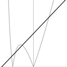
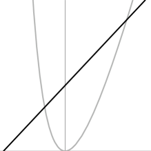
(a)	(b)

Figure 3: (a) $\psi$ and $\xi$ plotted as a function of $y$ for a classical black hole solution. The two horizons are at the zeroes of $\xi$ and the curvature singularity is where $\psi$ goes to zero. (b) In the extremal limit $\xi$ has a double zero at $y=0$ and the two horizons coincide.

In the extremal limit we have $\psi_{+}=\psi_{-}=M/2$ and the above solution reduces to

$$\psi(y) = \frac{M}{2}+\alpha y,$$ (26)

$$\xi(y) = \frac{8y^{2}}{M+2\alpha y}.$$ (27)

In this case there is a double horizon at $y=0$ and a curvature singularity at $y=-M/2\alpha$. The electric field at the double horizon of an extremal black hole is $f_{H}=\sqrt{8}$ for all values of $M$. The extremal solution is shown in Figure 3(b).

In the limit of neutral black hole we instead have $\psi_{+}=M$, $\psi_{-}=0$ and the classical solution takes the following simple form,

$$\psi(y)=M+\alpha y,\quad\xi(y)=\frac{4}{\alpha}|y|.$$ (28)

In this case there is only one horizon and the curvature singularity at $y=-M/\alpha$ is spacelike.

So far, we have only considered static classical solutions. In order to study charged black hole formation one would couple the dilaton gravity and gauge field to some form of charged matter and look for solutions of the classical equations of motion (2)–(4) with incoming matter energy and current. As far as we know, no closed form dynamical solutions to these equations exist. This is perhaps not surprising given that the system is known to exhibit intricate dynamical behavior, including a two-dimensional version of mass inflation Balbinot and Brady (1994); Chan and Mann (1994); Droz (1994). In the following section we couple the theory to charged matter but we do not pursue the problem of classical gravitational collapse. Instead we go on to include quantum effects in the form of pair-production of charged particles and then study the resulting semiclassical equations.

III Coupling to charged matter

In order to study the effect of Schwinger pair-production we add matter in the form of a 1+1-dimensional Dirac fermion $\Psi=\left(\begin{array}[]{c}\psi_{L}\\ \psi_{R}\end{array}\right)$ to the theory,

$$S_{m}=\int d^{2}x\sqrt{-g}\left[i\bar{\Psi}\gamma^{\mu}({\cal D}_{\mu}+ieA_{\mu})\Psi-m\bar{\Psi}\Psi\right]$$ (29)

where $e$ and $m$ are the charge and mass of our ‘electrons’, and ${\cal D}_{\mu}=\partial_{\mu}+\frac{i}{2}J_{ab}\omega^{ab}_{\phantom{ab}\mu}$ denotes a covariant derivative acting on 1+1-dimensional spinors. With this matter sector, our model can be viewed as a generalization to include gravitational effects in the ‘linear dilaton electrodynamics’ developed in Susskind and Thorlacius (1992); Peet et al. (1992); Alford and Strominger (1992). The current and energy-momentum carried by the fermions are given by

$$j^{\mu} = e\bar{\Psi}\gamma^{\mu}\Psi$$ (30)

$$T_{\mu\nu} = \frac{i}{4}\bar{\Psi}(\gamma_{\mu}{\cal D}_{\nu}+\gamma_{\nu}{\cal D}_{\mu})\Psi$$ (31)

$$- \frac{1}{2}g_{\mu\nu}(i\bar{\Psi}\gamma^{\lambda}({\cal D}_{\lambda}+ieA_{\lambda})\Psi-m\bar{\Psi}\Psi)$$

We could in principle look for dynamical solutions of the combined fermion and dilaton gravity system that describe classical black hole formation by an incoming flux of fermions. Our main interest is, however, in semiclassical geometries, with the back-reaction due to Schwinger pair-creation taken into account and this requires a different approach.

The key to including pair-creation is provided by the quantum equivalence between fermions and bosons in 1+1 dimensions. The massive Schwinger model, i.e. quantum electrodynamics of a massive Dirac particle in 1+1 dimensions, is equivalent to a bosonic theory with a Sine-Gordon interaction Coleman et al. (1975); Coleman (1976). In flat spacetime the identification between the fermion field and composite operators of a real boson field $Z$ is well known Coleman et al. (1975); Coleman (1976). This identification carries over to curved spacetime, with appropriate replacement of derivatives by covariant derivatives, as long as the gravitational field is slowly varying on the microscopic length scale of the matter system. The description in terms of bosons will break down in regions where the curvature gets large on microscopic length scales, i.e. near curvature singularities, but in such regions any classical or semiclassical description will be inadequate anyway.

In terms of the bosonic field the matter current is given by

$$j^{\mu}=\frac{e}{\sqrt{\pi}}\varepsilon^{\mu\nu}\nabla_{\nu}Z,$$ (32)

and the covariant effective action for the boson is

$$S_{b}=\int d^{2}x\sqrt{-g}\left[-\frac{1}{2}(\nabla Z)^{2}-V(Z)-\frac{e}{\sqrt{4\pi}}\varepsilon^{\mu\nu}F_{\mu\nu}Z\right],$$ (33)

where $V(Z)=c\,e\,m(1-\cos(\sqrt{4\pi}Z))$, with $c$ a numerical constant whose precise value does not affect our considerations. In order to model real electrons our fermions should have a large charge-to-mass ratio. In this case the fermion system is highly quantum mechanical but, since the fermion-boson equivalence in 1+1 dimensions is an example of a strong/weak coupling duality, the boson system is classical precisely when $m\ll e$. For simplicity, we set $m=0$ in most of what follows, but our numerical results below include runs with $m>0$.

IV Semiclassical equations

We obtain the semiclassical geometry of a two-dimensional black hole by solving the equations of motion of the combined boson and dilaton gravity system, (1) and (33). We consider both dynamical collapse solutions and static solutions that describe eternal black holes. For the dynamical solutions it is convenient to work in conformal gauge with null coordinates $ds^{2}=-e^{2\rho}d\sigma^{+}d\sigma^{-}$. Writing $F^{\mu\nu}=f\varepsilon^{\mu\nu}$ as before, the Maxwell equation (4), including the bosonized matter current (32), becomes

$$\partial_{\pm}(e^{-2\phi}f+\frac{e}{\sqrt{\pi}}Z)=0.$$ (34)

Once again the gauge field can be eliminated,

$$f=\frac{1}{\psi}\left(-\frac{e}{\sqrt{\pi}}Z+q\right).$$ (35)

By comparing to the classical result (18) we see that the value of the bosonic field $Z$ at a given spatial location determines the amount of electric charge to the left of that location, or ‘inside’ it from the 3+1-dimensional point of view. There is also an integration constant $q$ that represents a background charge located at the strong coupling end of the one-dimensional space. In the following we will set $q=0$. This is natural when we consider gravitational collapse of charged matter into an initial vacuum configuration. Furthermore, if we assume that the background charge $q$ is an integer multiple of the fundamental charge $e$ carried by our fermions, then it can be set to zero by a symmetry of the semiclassical equations under a discrete shift of $Z$ by $\sqrt{\pi}$ times an integer. For $m=0$ the shift symmetry becomes continuous and in that case an arbitrary background charge, and not just integer multiples of $e$, can be absorbed by a shift of $Z$. For convenience we adopt units in which $e=1$ in the remainder of this paper.

We now insert expression (35) for the gauge field, with $q=0$ and $e=1$, into the remaining semiclassical equations. They are somewhat simplified if we introduce $\theta=2(\rho-\phi)$ and work with the area function $\psi$ instead of the dilaton field itself. The resulting system of equations is

$$-4\partial_{+}\partial_{-}\psi = \left(4-\frac{Z^{2}}{2\pi\psi^{2}}\right)e^{\theta}-\frac{V(Z)e^{\theta}}{\psi},$$ (36)

$$-4\partial_{+}\partial_{-}\theta = \frac{Z^{2}e^{\theta}}{\pi\psi^{3}}+\frac{V(Z)e^{\theta}}{\psi^{2}},$$ (37)

$$-4\partial_{+}\partial_{-}Z = \frac{Ze^{\theta}}{\pi\psi^{2}}+\frac{V^{\prime}(Z)e^{\theta}}{\psi},$$ (38)

along with two constraints

$$\partial_{\pm}^{2}\psi-\partial_{\pm}\theta\partial_{\pm}\psi=-\frac{1}{2}(\partial_{\pm}Z)^{2}.$$ (39)

Equations (36)–(39) can be solved numerically with initial data that describes charged matter undergoing gravitational collapse. In section VI we employ a finite difference algorithm to study this process but let us first consider the simpler problem of static solutions of the semiclassical equations that describe eternal black holes.

V Static black holes

For static configurations of the semiclassical equations (36)–(39) we require the fields to depend only on the spatial variable $\sigma=\frac{1}{2}(\sigma^{+}-\sigma^{-})$. To study such solutions we proceed as in the classical theory, writing $\xi=e^{\theta}$ and defining a new spatial coordinate via $dy=\xi d\sigma$. Outside the event horizon the semiclassical equations (36)–(37) reduce to

$$\xi\ddot{\psi}+\dot{\xi}\dot{\psi} = 4-\frac{Z^{2}}{2\pi\psi^{2}}-\frac{V(Z)}{\psi},$$ (40)

$$\ddot{\xi} = \frac{Z^{2}}{\pi\psi^{3}}+\frac{V(Z)}{\psi^{2}},$$ (41)

$$\xi\ddot{Z}+\dot{\xi}\dot{Z} = \frac{Z}{\pi\psi^{2}}+\frac{V^{\prime}(Z)}{\psi},$$ (42)

where the dots once again denote derivatives with respect to $y$. The constraints (39) become

$$\ddot{\psi}+\frac{1}{2}(\dot{Z})^{2}=0.$$ (43)

At first sight, it appears that we have four equations for only three fields, but the equations are not independent. Inserting (43) into (40) gives

$$-\frac{1}{2}\xi\dot{Z}^{2}+\dot{\xi}\dot{\psi}=4-\frac{Z^{2}}{2\pi\psi^{2}}-\frac{V(Z)}{\psi},$$ (44)

which is easily seen to be a first integral of equations (41)–(43).

Inside the event horizon $y$ becomes timelike which means that the derivative terms in equations (40)–(42) change sign in that region.

$$-\xi\ddot{\psi}-\dot{\xi}\dot{\psi} = 4-\frac{Z^{2}}{2\pi\psi^{2}}-\frac{V(Z)}{\psi},$$ (45)

$$-\ddot{\xi} = \frac{Z^{2}}{\pi\psi^{3}}+\frac{V(Z)}{\psi^{2}},$$ (46)

$$-\xi\ddot{Z}-\dot{\xi}\dot{Z} = \frac{Z}{\pi\psi^{2}}+\frac{V^{\prime}(Z)}{\psi},$$ (47)

The semiclassical equations are more complicated than the classical ones and explicit analytic solutions are not available. They can, however, be integrated numerically to obtain information about the semiclassical geometry of charged black holes.

V.1 Numerical black hole solutions

In order to find a numerical black hole solution which is well behaved at the event horizon we start our integration at $y=0$ and set $\xi(0)=0$. Different black holes are parametrised by the initial values $Z(0)$ and $\psi(0)$. Second order equations also require initial values for first derivatives of the fields. The choice of $\dot{\xi}(0)$ does not affect the geometry but instead sets the scale of the spatial coordinate $y$. The remaining two initial values are provided by the equations themselves when we impose the condition that the solution be regular at the event horizon Birnir et al. (1992). By setting $\xi(0)=0$ in equations (40) and (42) for the exterior solution (equations (45) and (47) for the interior solution) while requiring that $\ddot{\psi}$ and $\ddot{Z}$ are finite at $y=0$, we obtain

$$\dot{\psi}(0) = \frac{1}{|\dot{\xi}(0)|}\left(4-\frac{Z(0)^{2}}{2\pi\psi(0)^{2}}-\frac{V(Z(0))}{\psi(0)}\right),$$ (48)

$$\dot{Z}(0) = \frac{1}{|\dot{\xi}(0)|}\left(\frac{Z(0)}{\pi\psi(0)^{2}}+\frac{V^{\prime}(Z(0))}{\psi(0)}\right).$$ (49)

The exterior solution is found by starting with these initial values at the black hole horizon at $y=0$ for some $\dot{\xi}(0)>0$ and integrating equations (40)-(42) numerically towards $y>0$. For the integration into the black hole we instead use equations (45)-(47) and change the sign of $\dot{\xi}(0)$.

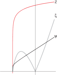
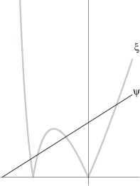
(a)	(b)

Figure 4: (a) $\psi$, $\xi$, and $Z$ plotted as a function of $y$ for a semiclassical black hole. The inner horizon of the classical solution is replaced by a singularity where $\psi$, $\xi$, and $Z$ all approach zero. (b) A corresponding plot for a classical black hole solution, repeated from Figure 3 for comparison.

Typical numerical results for massless matter are shown in Figure 4a. We have also numerically integrated the equations with a non-vanishing fermion mass $m$ and find the same qualitative behavior for small $m$. For large values of $m$ the bosonic theory is strongly coupled and our semiclassical equations can no longer be trusted.

The scalar fields $\psi$ and $Z$ extend smoothly through the horizon at $y=0$, while $\xi$ goes to zero there and $\dot{\xi}$ changes sign, as in the classical theory. Away from the horizon we see important departures from the classical solution. We will discuss the exterior region below but let us first consider the interior of the black hole where the semiclassical solution is dramatically different from the classical geometry.

V.2 Black hole region

In the classical black hole solution (24)–(25) the area function $\psi$ goes linearly to zero with negative $y$ inside the event horizon. The falloff of $\psi$ is more rapid in the corresponding semiclassical solution. This can be traced to pair-creation of charged fermions in the black hole interior, which causes the amplitude of the bosonized matter field to decrease as we go deeper into the black hole. From the constraint equation (43) we see that $\psi$ is a concave function and any variation in $Z$ serves to focus it towards zero. The conformal factor of the metric is contained in the $\xi$ field. Inside the event horizon at $y<0$ the left hand side of (41) changes sign and as a result the $\xi$ field is also concave in this region. Initially, $\xi$ grows away from zero at the horizon as we go towards negative $y$ but eventually it turns over and approaches zero again at a finite negative value $y=-y_{0}$.

This second zero of $\xi$ does not correspond to a smooth inner horizon, as can be seen from the following argument. Finiteness of $\ddot{\psi}$ and $\ddot{Z}$ at $y=-y_{0}$ would require

$$\dot{\psi}(-y_{0}) = -\frac{1}{\dot{\xi}(-y_{0})}\left(4-\frac{Z(-y_{0})^{2}}{2\pi\psi(-y_{0})^{2}}\right),$$ (50)

$$\dot{Z}(-y_{0}) = -\frac{1}{\dot{\xi}(-y_{0})}\left(\frac{Z(-y_{0})}{\pi\psi(-y_{0})^{2}}\right),$$ (51)

where we have set the fermion mass $m$ to zero for simplicity. Since $\dot{\xi}(-y_{0})>0$ as $y\rightarrow-y_{0}$ it follows from equation (51) that

$$\frac{d}{dy}\log|Z|<0,\qquad\textrm{as}\qquad y\rightarrow-y_{0},$$ (52)

while the same quantity is positive at $y=0$. This sign change can occur in one of two ways, shown in Figure 5.

\psfrag{y}{$y$}\psfrag{y0}{$-y_{0}$}\psfrag{Z}{$Z$}\includegraphics[width=108.12054pt]{figs/signZa}	\psfrag{y}{$y$}\psfrag{y0}{$-y_{0}$}\psfrag{Z}{$Z$}\includegraphics[width=108.12054pt]{figs/signZb}
(a)	(b)

Figure 5: Two cases in which the sign change of equation (52) occurs. (a) The field $Z$ has a local minimum at some $y$ in the interval $-y_{0}<y<0$, or (b) the field $Z$ goes through zero at some $y$ in the same interval.

Assuming $Z(0)>0$ (a parallel argument can be given for $Z(0)<0$) we either have a local minimum of $Z$ at some $y$ in the interval $-y_{0}<y<0$, as in Figure 5a, or $Z$ goes through zero at some $y$ in the same interval, as in Figure 5b. A local minimum for $Z$ is easily ruled out. Inserting $\dot{Z}=0$ into equation (47) with $Z>0$ we find that $\ddot{Z}<0$, which corresponds to a local maximum rather than a minimum. The other possibility, i.e. $Z$ going through zero, can be eliminated on physical grounds, because it would correspond to the charge inside a given location changing sign. Screening due to pair production will reduce the charge as one goes deeper into the black hole but cannot change its sign. We cannot rule out that non-linear effects in a strong coupling region close to a curvature singularity could reverse the sign of $Z$, but the above argument does rule out the possibility of having an inner horizon with macroscopic area.

We conclude from this that the solution will not be smooth as $\xi\rightarrow 0$ inside the black hole and this is borne out by our numerical calculations. We find that all the fields $\xi$, $\psi$ and $Z$ are simultaneously driven to zero while their derivatives become large. The Ricci scalar

$$R=-\xi\ddot{\psi}-\dot{\xi}\dot{\psi}+\ddot{\xi}\psi+\frac{\xi\dot{\psi}^{2}}{\psi^{2}},$$ (53)

evaluated for the numerical solution, increases rapidly as we approach the singular point. This indicates that the classical inner horizon is replaced by a curvature singularity at the semiclassical level. The numerical solution breaks down before an actual singularity is reached, but as far as the numerical evidence goes, it indicates that the singularity is spacelike. In section VI we will present numerical evidence that the singularity formed in dynamical gravitational collapse in this model is also spacelike.

We have found a two-parameter family of singular scaling solutions, which is a candidate for the final approach to the singularity,

$$\psi(y) = A(y+y_{0})[-\log(y+y_{0})]^{a},$$ (54)

$$\xi(y) = \frac{4}{\pi A^{2}}[-\log(y+y_{0})]^{-2a},$$ (55)

$$Z(y) = \pm\sqrt{8aA}(y+y_{0})^{1/2}[-\log(y+y_{0})]^{(a-1)/2},$$ (56)

Here $y=-y_{0}$ is the coordinate location of the singularity, which depends on the global coordinate scale set by $\dot{\xi}(0)$ in equations (48) and (49). We emphasize that this singular solution is at best asymptotic to the true solutions near the singularity, since it only equates the most singular terms in the semiclassical equations, leaving behind terms that are sub-leading but nevertheless divergent. The neglected sub-leading terms are only logarithmically suppressed compared to the leading terms and this means that we are unable to match our numerical solution onto the proposed scaling solution. A successful match would either involve following the numerical solution extremely close to the singularity, far beyond presently attainable numerical precision, or working out several subleading orders in the scaling solution, which is beyond our analytic perseverance. In the absence of successful matching we can only tentatively claim that our scaling solution correctly describes the geometry near the singularity, but let us nevertheless investigate some of its properties.

The Ricci scalar (53) is easily seen to diverge as $y\to-y_{0}$ in the scaling solution (54)–(56) so the singular point represents a true curvature singularity. The singularity is in fact strong, in the sense that not only does the curvature itself blow up there but also its integral along a timelike geodesic approaching $y=-y_{0}$. This indicates that both the tidal force acting on an extended observer and the integrated tidal force will diverge as the singularity is approached.

The conformal factor of the metric, which is given by the ratio $\xi/\psi$, diverges as $y\to-y_{0}$. A singularity described by equations (54)–(56) is therefore spacelike rather than null. The area function $\psi$ goes to zero as the singularity is approached in both the numerical solution and our proposed scaling solution. This means that the gravitational sector becomes infinitely strongly coupled at the curvature singularity.

V.3 Exterior region

The spacelike singularity encountered in the black hole interior is the most important feature of our semiclassical solutions but it is useful to consider also the region far away from the black hole. Understanding the asymptotic behavior of the solutions provides a check on our formalism. In this region the coupling strength $e^{\phi}$ goes to zero and the gravitational fields $\psi$ and $\xi$ should approach classical behavior. Both $\psi$ and $\xi$ grow linearly with $y$ in the classical solution (24)–(25). The corresponding semiclassical fields also grow linearly at large $y$ but have additional logarithmic terms. The static equations (40)–(43) are solved to leading order at large $y$ by

$$Z(y) = Z_{0}\log(\alpha y)+\cdots$$ (57)

$$\psi(y) = \alpha y+\frac{Z_{0}^{2}}{2}\log(\alpha y)+\cdots$$ (58)

$$\xi(y) = \frac{4}{\alpha}y+\xi_{0}\log(\alpha y)+\cdots$$ (59)

where the $\cdots$ denote terms that are constant or vanish in the limit.

As a result of the logarithmic growth of $Z$ there is a non-vanishing energy density in matter in the asymptotic region and, via equation (32), a finite electric charge density also. The ADM total mass and total charge of these black hole geometries are therefore infinite. At first sight, one might expect that an infinite amount of matter energy will collapse the geometry, but the gravitational coupling goes to zero in the asymptotic region so the matter in fact decouples from the gravitational sector. In two spacetime dimensions we can interpret a non-vanishing asymptotic energy density of massless matter in a static solution in terms of balanced incoming and outgoing energy fluxes carried by particles in the limit of zero momentum Peet et al. (1993). In our case, the elementary fermions carry electric charge so there is also a balance between outgoing and incoming electric flux.

The outgoing flux is due to pair-production in the electric field outside the event horizon of the black hole. Particles carrying charge of opposite sign to that of the black hole are electrically attracted to the hole while same sign charges are repelled. This leads to a net flow of charge and energy away from the black hole but since we are considering static solutions this flow is balanced by an equal influx from an external source at infinity. This is reminiscent of the so-called quantum black hole solutions of Birnir et al. (1992) and the interpretation is similar, except in that case the outgoing energy flux at infinity is in the form of Hawking radiation rather than charged particles formed by pair-production.

The asymptotic matter energy density, measured with respect to an asymptotically Minkowskian coordinate frame, is given by

$$\varepsilon=\lim_{y\rightarrow\infty}\frac{1}{2}\psi\xi\left(\frac{dZ}{dy}\right)^{2},$$ (60)

which reduces to $\varepsilon=2Z_{0}^{2}$ for the semiclassical fields in equations (57)–(59). The value of $\varepsilon$ for a given semiclassical black hole is easily obtained from the numerical solution and the results are plotted in Figure 6. The data clearly show that the energy density depends on the electric field at the black hole horizon but is independent of the overall size of the black hole for a fixed electric field. We are using equation (35) to define the electric field strength at the horizon as 

$$f(0)=\frac{Z(0)}{\sqrt{\pi}\psi(0)}.$$ (61)

\psfrag{eps}{$\varepsilon$}\psfrag{f}{$f(0)/\sqrt{8}$}\psfrag{psi}{$\psi(0)$}\includegraphics[width=173.44865pt]{figs/energydensity}

(a)
\psfrag{eps}{$\varepsilon$}\psfrag{f}{$f(0)/\sqrt{8}$}\psfrag{psi}{$\psi(0)$}\includegraphics[width=173.44865pt]{figs/energydensity2}               (b)

Figure 6: (a) The asymptotic energy density $\varepsilon$ as a function of the electric field at the horizon $f(0)$. (b) The asymptotic energy density $\varepsilon$ as a function of $\psi(0)$ for four values of $f(0)/\sqrt{8}=0.2,0.4,0.6,0.8$.

For massless fermions the exponential suppression of Schwinger pair-production is absent and the pair production rate per proper volume depends on the electric field strength as a power law. In two spacetime dimensions this dependence is linear but this is only part of the story. Particles are created at every distance from the black hole, although most of them come from near the horizon where the electric field is strongest, and those particles that carry the same sign charge as the black hole are then accelerated out to infinity by the electric field. These particles, along with a corresponding influx of energetic particles to maintain the static nature of the solution, make up the asymptotic matter energy density $\varepsilon$. The dots in Figure 6(a) are results from numerical integrations while the solid line is given by a curve $\varepsilon\sim f(0)^{2}$. The close fit shows that the energy density at infinity goes like the electric field strength at the horizon squared.

V.4 Maximally charged black holes

At the classical level the extremal black hole of mass $M$ carries the maximum possible charge for a black hole of that mass. Adding more charge, keeping the mass fixed, results in a naked singularity instead of a black hole. The geometry of an extremal black hole is qualitatively different from that of a non-extremal black hole in the classical theory. The two horizons have merged into a double horizon which is located at infinite proper distance from fiducial observers outside the black hole. This picture is modified in the semiclassical theory with $m=0$ where we find that there is again a maximum charge that can by carried by a black hole of a given mass but the corresponding geometry is not extremal.

The absence of extremal black holes is explained by the screening effect of charged pairs produced in the electric field outside the black hole. Recall from equation (43) that $\psi$ is a concave function of $y$ and in order for the spacetime to be asymptotically flat $\psi$ must remain a growing function of $y$ in the asymptotic region $y\to\infty$. If the charge-to-mass ratio of the semiclassical black hole becomes too large the solution collapses to $\psi=0$ at a finite distance outside the horizon and the geometry is no longer that of a black hole. This is most conveniently analyzed in terms of the electric field at the black hole horizon, $f(0)$, which is bounded from above in the classical limit by the field of an extremal black hole, $f(0)\leq\sqrt{8}$. A close look at our numerical solutions reveals that $\psi$ will collapse far away from the black hole unless the electric field at the horizon satisfies

$$\frac{f(0)}{\sqrt{8}}<1-\frac{1}{8\pi\psi(0)}+{\cal O}\left(\frac{1}{\psi(0)^{2}}\right),$$ (62)

which is lower than the classical maximum. By looking at equation (48) for $m=0$ (and therefore $V(Z)=0$) we see that $\dot{\psi}(0)>0$ for all $f(0)<\sqrt{8}$ but if the electric field at the horizon is in the range

$$1-\frac{1}{8\pi\psi(0)}+{\cal O}\left(\frac{1}{\psi(0)^{2}}\right)<\frac{f(0)}{\sqrt{8}}<1$$ (63)

for large $\psi(0)$, then $\dot{\psi}$ changes sign at some $y>0$ and the solution collapses to $\psi=0$.

The interior geometry of any semiclassical black hole, for which the electric field at the horizon is below the maximal value in equation (62), looks like the typical solution in Figure 3(b). In particular there is no sign of the double horizon of the classical extremal black hole in Figure 4(b). We conclude that the energy density of pair-created particles outside a two-dimensional charged black hole will collapse the geometry before the extremal limit is reached.

VI Dynamical collapse

In this section, we study the problem of dynamical collapse of a charged matter distribution by solving the semiclassical equations (36)–(39) numerically. It is the internal structure of the resulting black hole that is of prime interest to us. We must therefore choose our coordinate system carefully (it should penetrate horizons) and select a numerical method which avoids propagating information faster than true characteristic speed of the equations. We employ a grid based on double-null coordinates $(u,v)$ and discretize the second-order equations of motion (36)–(38) using a variation of a leapfrog algorithm.

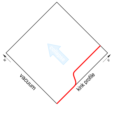
Figure 7: Initial data for dynamical collapse.

The initial data for the null Cauchy problem is specified by providing the values of the functions $\psi$, $\theta$, and $Z$ on a double-null wedge, as shown in Figure 7. Only one of the three functions is physical and we have chosen this to be the bosonized matter field $Z$. The area function $\psi$ can be fixed by a choice of null coordinate parametrization on the initial wedge and then the remaining function $\theta$ is determined by solving the constraint equation (39).

The physical initial condition is the initial incoming charge distribution $Z$, which we take to be a smooth kink profile

$$Z(0,v)=\frac{Q}{2}\left[\tanh\left(w\tan\pi\big{(}{\textstyle\frac{v-v_{1}}{v_{2}-v_{1}}-\frac{1}{2}}\big{)}\right)+1\right]$$ (64)

collapsing into a previously empty spacetime with $Z(u,0)=0$, as illustrated by Figure 7. The kink in the profile is localized between $v_{1}$ and $v_{2}$. It carries a total charge $Q$ and an energy density determined by its gradient squared, so the total mass scales roughly as $Q^{2}w$.

The null coordinate choice is effectively given by a choice of $\psi$ profile on the initial wedge. As the vacuum solution takes a particularly simple form in a gauge

$$\psi(u,v)=-(u-u_{0})(v-v_{0}),\hskip 10.00002pt\theta(u,v)=0,$$ (65)

one is tempted to take $\psi(u,0)$ and $\psi(0,v)$ as linear functions of $u$ and $v$ respectively. However, in order to cover the entire spacetime by a finite grid, we compactify the $v$ coordinate by taking, for example, $\psi(0,v)=\psi_{0}+\alpha\tan kv$. Here $v$ runs over the range $[0,1]$ and the parameter $k<\pi/2$ provides a regulator for $\psi$ as $v\rightarrow 1$. On the other hand, we leave $\psi(u,0)$ linear in $u$. With incoming matter we expect a curvature singularity to form at $\psi=0$ and since $\psi(u,0)$ has a zero at a finite advanced time $u=u_{0}$ there is no need to compactify the $u$ coordinate.

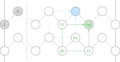
Figure 8: The numerical evolution scheme is a a staggered grid leapfrog.

The remaining function $\theta$ is determined by fourth order fixed step Runge-Kutta integration of the constraint equation (39) on the initial slice $u=0$. We also integrate $\partial_{u}$ and $\partial_{uu}$ derivatives, which are then used to jump-start the two-dimensional evolution.

The numerical evolution scheme is a leapfrog algorithm on a staggered grid, which is illustrated by Figure 8. The values of functions at a given $u$ are stored in an array, and are propagated to the next time step $u+\epsilon$ using the equations of motion, except for the leftmost values, which are filled in using the vacuum initial conditions at $v=0$. The differential operators on the left hand sides of equations (36)–(38) are discretized as

$$-\partial_{u}\partial_{v}X=\frac{1}{\epsilon^{2}}(X_{\text{lt}}+X_{\text{rt}}-X_{\text{dn}}-X_{\text{up}}),$$ (66)

which gives a second order accurate expression in the center of the cell formed by $X_{\text{lt}}$, $X_{\text{up}}$, $X_{\text{dn}}$, and $X_{\text{rt}}$. This is why the staggered grid was chosen – it provides the values of the fields at the correct location for evaluation of the right hand sides. One can think of the staggered grid as a square grid rotated by forty five degrees. Then the discretization (66) is readily recognized as the usual leapfrog discretization of the wave operator $-\partial_{t}^{2}+\partial_{x}^{2}$.

(a) $Z(u,v)$, $m=0$	(b) $Z(u,v)$, $m=0.05$
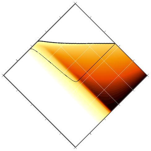
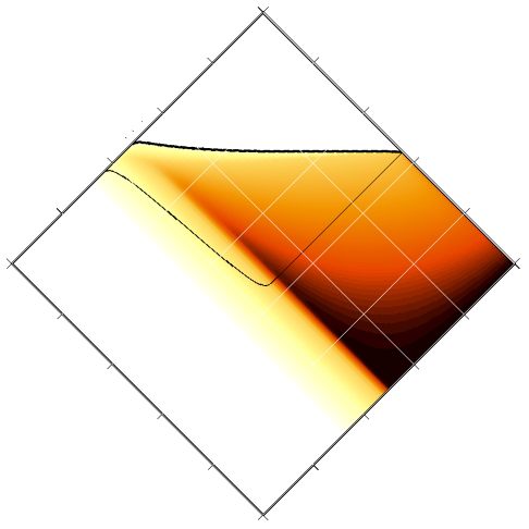
(c) $\psi(u,v)$, $m=0$	(d) $R(u,v)$, $m=0$

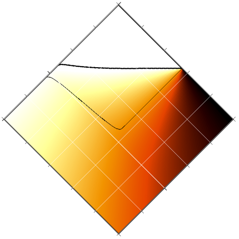
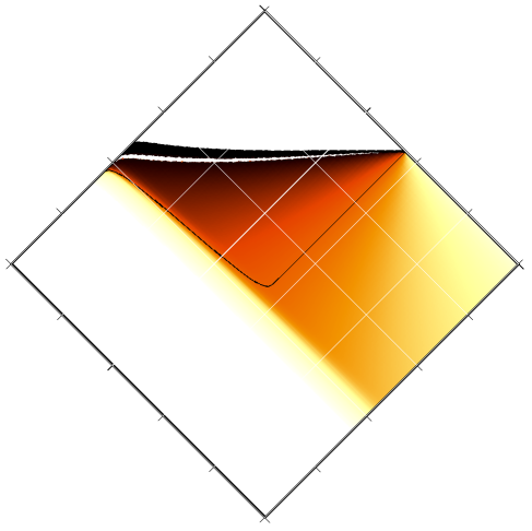
Figure 9: Density plots of the charge distribution $Z(u,v)$ for the collapse of massless (a) and massive (b) fermions. The density plots of (c) dilaton $\psi(u,v)$ and (d) scalar curvature $R(u,v)$ are for collapse of massless fermions. The corresponding plots for collapse of massive fermions are not substantially different, and are not provided here. The singularity is shown by a thick black line, while the thin line indicates the apparent horizon. The white stripe just below the singularity in (d) is region of negative curvature.

VI.1 Numerical results

We now present results obtained from numerical evolution using the above algorithm and initial data of the type shown in Figure 7. The results are exhibited as density plots of the various fields with shading intensity giving the value of the field in question. To facilitate the interpretation of the numerical data we indicate curvature singularities in the plots by thick black curves and apparent horizons by thin black curves. The local condition for a future trapped event is that the area function be decreasing along both future null directions,

$$\partial_{\pm}\psi<0.$$ (67)

The apparent horizon is located at the boundary of such a region, i.e. where $\partial_{+}\psi=0$ or $\partial_{-}\psi=0$ Russo et al. (1992).

Figure 9(a) shows the charge distribution $Z(u,v)$ in a spacetime where matter in the form of massless fermions undergoes gravitational collapse. Observe how $Z\rightarrow 0$ deep inside the black hole, which can be attributed to charge screening due to fermion pair production. One can also see the (slow) discharge of a black hole by pair production at the horizon. The shading scheme is exaggerated to show this more clearly. For comparison, Figure 9(b) shows the collapse resulting from the same initial conditions, but for massive fermions. In this case, the charge penetrates deeper into the black hole before pair production can screen it efficiently. The geometry of the spacetime is not substantially different for the massless and massive cases and is only shown for the former. Figure 9(c) depicts the dilaton field $\psi(u,v)$, while Figure 9(d) shows the scalar curvature $R(u,v)$ with compressed shading to span a huge range. From these plots one clearly sees the formation of a spacelike curvature singularity in the black hole interior and there is no indication of a null singularity or a Cauchy horizon.

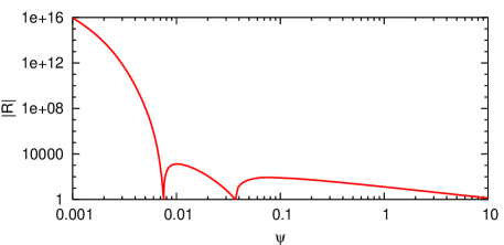
Figure 10: Spacetime curvature along a constant $v$ profile that runs into the black hole singularity.

The white stripe preceding the singularity in the curvature plot in Figure 9(d) is a region of negative curvature, which the plot program treats as missing data. This oscillation in the spacetime curvature is also seen in Figure 10 which shows the curvature along a profile at fixed retarded time, $v=$constant. The figure is a log-log plot of $|R|$ against $\psi$ along the profile and the middle hump is in the region of negative curvature.

VI.2 Scaling behavior

Rather remarkable critical behavior occurs at the onset of black hole formation in gravitational collapse in classical Einstein gravity coupled to a massless scalar field Choptuik (1993). A sufficiently weak ingoing s-wave pulse reflects from the origin without creating a black hole but above a certain critical threshold, as the amplitude of the pulse is increased, a black hole will form. Near this threshold the black hole mass obeys a scaling law,

$$\log M=\gamma\log\delta+O(\delta^{0}),$$ (68)

where $\delta$ parametrizes the distance from the threshold in the initial data and $\gamma\approx 0.37$ is a scaling exponent obtained from numerical data Choptuik (1993).

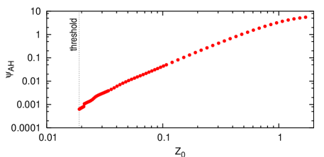
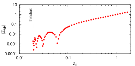
Figure 11: Scaling behavior of the area of the apparent horizon.

Figure 12: The absolute value of $Z_{\text{AH}}$, the bosonized matter field at the apparent horizon, in the scaling regime. The sign of $Z_{\text{AH}}$ changes between adjacent humps in the graph.

We have looked for analogous scaling behavior in the formation of charged black holes in our semiclassical model. Figure 12 shows the area of the apparent horizon that forms in gravitational collapse of charged matter as a function of the amplitude of the incoming kink profile. A close look at the numerical data indicates that there is indeed a threshold for black hole formation, which we find by bisection. The data also suggest that black hole formation turns on at finite size, which is reminiscent of the Type I critical behaviour found in gravitational collapse of a Yang-Mills field in Einstein gravity Choptuik et al. (1999). For a super-critical collapse, the size of the black hole can be fitted by a power law

$$\psi_{\text{AH}}\propto(Z_{0}-Z_{*})^{\gamma_{Z}}\,,$$ (69)

where $Z_{0}$ is the amplitude of the initial kink, and the scaling exponent is

$$\gamma_{Z}=1.85\pm 0.01\,.$$ (70)

We have also considered a family of initial data where the width parameter $w$ of the kink profile in equation (64) is varied rather than its height. We again find scaling behavior,

$$\psi_{\text{AH}}\propto(w-w_{*})^{\gamma_{w}}\,,$$ (71)

but with a different scaling exponent

$$\gamma_{w}=0.71\pm 0.03\,,$$ (72)

so it appears that the scaling exponent is not universal. We should note that the best-fitting offset values $Z_{*}$ and $w_{*}$ are substantially less than the actual threshold values.

By equation (35) the bosonized matter field $Z$ determines the amount of charge to the left of, or inside, a given location. It is therefore straightforward to consider the initial black hole charge, which we define as the charge inside the apparent horizon when the black hole forms, for initial data in the scaling regime. The results, presented in Figure 12, show more complicated behavior than that of the black hole area. The black hole charge appears to show an overall power-law scaling, but the sign of the charge starts oscillating and the power-law exponent steepens as the threshold is approached. It would be interesting to understand this behavior better.

VII Discussion

We have studied the geometry of charged black holes in the context of a 1+1-dimensional model of dilaton gravity with charged matter in the form of bosonized fermions. At the classical level, the model has static black hole solutions with a global causal structure identical to the four-dimensional Reissner-Nordström solution. When the quantum effect of pair-production of charged particles is taken into account the classical inner horizon is replaced by a spacelike singularity and the global structure of the spacetime geometry is that of an electrically neutral black hole.

This result is based on a combination of numerical and analytic analysis of semiclassical equations of motion, both static and dynamical. The static solutions are being constantly fed by an external source to balance quantum mechanical black hole evaporation and discharge. The dynamical solutions, on the other hand, describe the collapse of charged matter into vacuum.

The strong form of the cosmic censor conjecture Penrose (1979) forbids naked singularities to be visible to any physical observers, including ones who travel inside charged black holes. Our semiclassical results clearly support strong cosmic censorship, while its validity for charged black holes in classical gravity is a delicate issue Ori (1991); Dafermos (2003).

We believe our two-dimensional model captures some of the essential physics of this problem while leaving out many of the complications of the full higher-dimensional quantum gravity problem. The model is certainly not without fault, it has no propagating gravitons or photons and the electric field of a black hole only depends on the charge to mass ratio of the black hole, but as far as we know there exists no systematic treatment of quantum effects, including pair-production of charged particles, for higher-dimensional black holes.

Our results can be improved on in a number of ways. For example, we have not included gravitational quantum effects in our two-dimensional model in this paper. There exists an extensive literature on semiclassical two-dimensional dilaton gravity, including the Hawking effect and its back-reaction on the geometry of neutral black holes. For reviews see Giddings (1994); Strominger (1994); Thorlacius (1995); Grumiller et al. (2002); Fabbri and Navarro-Salas (2005). We expect that gravitational back-reaction to Hawking radiation will not change our main conclusion that the singularity formed in the gravitational collapse of charged matter is spacelike. Subtleties involving boundary conditions in the strong coupling region complicate the problem but a preliminary numerical study of charged black hole formation, with the combined effect of pair-production and electrically neutral Hawking emission included, confirms this expectation Kristjansson (2005). Quantum effects due to electrically neutral matter in a charged black hole spacetime have been considered by a number of authors, see for example Trivedi (1993); Frolov et al. (1996); Diba and Lowe (2002); Zaslavskii (2004). However, pair-production is not considered in these papers.

One might also worry about the phenomenological relevance of charged black holes in general. It is after all very unlikely that black holes carrying macroscopic electric charge are found in Nature. Solutions that describe such objects do, however, exist in the theories we use to describe Nature and they provide an important testbed for theoretical ideas. Furthermore, issues of Cauchy horizons and non-trivial global topology of spacetime also arise in the context of rotating black holes, which presumably are the generic black holes of astrophysics.