A Fermi Surface Model for Large Supersymmetric AdS₅ Black Holes

Abstract:

We identify a large family of 1/16 BPS operators in $\mathcal{N}=4$ SYM that qualitatively reproduce the relations between charge, angular momentum and entropy in regular supersymmetric AdS₅ black holes when the main contribution to their masses is given by their angular momentum.

1 Introduction

One of the successes of string theory is the statistical mechanics derivation of the entropy of supersymmetric black holes [1]. In particular, within the context of the AdS/CFT correspondence [2, 3, 4, 5], one can carry out detailed computations of black hole properties and compare them to results from the dual conformal field theory.

One of the most heavily studied cases of the AdS/CFT is the duality between type IIB string on $AdS_{5}\times S^{5}$ to $\mathcal{N}=4$ SYM. In this case, however, black hole entropy counting has turned out to be tricky. For large non-supersymmetric black holes $S=cN^{2}T^{3}$ [6]. The power of $T$ is determined by dimensional analysis, $N^{2}$ is the free theory scaling of degrees of freedom, but the coefficient, $c$, can not be computed reliably [7, 8]. In the arena of supersymmetric R-charged configurations, there are no honest black holes in the $1/2$ to $1/{8}$-BPS sector states, i.e, there is less than $N^{2}$ worth of entropy, and so their horizons are Planck scale.

In the current paper we take some first steps towards understanding the AdS/CFT correspondence in cases with $1/16$ SUSY. With this amount of supersymmetry, there is a rich spectrum of genuine black holes with smooth horizons and non vanishing angular momentum [9, 10, 11, 12]. Our goal is to, first, find their field theory duals (forcing us to understand the addition of angular momentum), and second, to count them. In this paper we explain some structures which are key to the construction of the $1/16$ operators in the CFT. Our construction is based on the filling of fermi surfaces, and it is similar in spirit to the construction in terms of free fermions for the $1/2$ - $1/8$ BPS states [13, 14, 15, 16]. Using this structure we reproduce the scalings between angular momentum, charge and entropy of $1/16$ SUSY black holes, up to coefficients of order 1. Furthermore, since the fermi surface is multi-dimensional, it posses a complicated morphology. This suggests that additional types of black holes might be constructed, with an equally complicated bulk morphology.

Asymptotically supersymmetric AdS₅ black holes were originally constructed in [9, 10] and later generalized in [11, 12]. These black holes carry both angular momenta $\{J,\,\bar{J}\}$ under $\operatorname{SU}(2)_{L}\times\operatorname{SU}(2)_{R}$ and $\operatorname{SO}(6)$ R-charges $\{Q_{1},\,Q_{2},\,Q_{3}\}$. Their mass is given by the BPS equation:

$$M=\frac{2J}{l}+Q_{1}+Q_{2}+Q_{3}\,.$$ (1)

The $Q_{i}$’s are taken to be of dimension 1, and $l$ is the AdS₅ radius.

There are two natural scaling regimes to consider according to whether the R-charge or the angular momenta is large. In this note, we study the regime in which the black hole mass is dominated by the angular momenta. For simplicity, we focus on black holes having three equal $\operatorname{SO}(6)$ R-charges $Q_{1}=Q_{2}=Q_{3}=\frac{Q}{2\sqrt{3}}$. Black holes in this regime exhibit different angular momentum-charge relations depending on their right handed angular momentum, $\bar{J}$ (which does not appear in the BPS formula). The two scaling behaviors that we will be interested in

$$J/N^{2}\sim (Q/N^{2})^{3/2}, \text{if}\qquad\bar{J}\simeq 0\hskip 10.00002pt,\hskip 10.00002ptQ>>N^{2}\,,$$ (2)

$$J/N^{2}\sim (Q/N^{2})^{2}, \text{if}\qquad\bar{J}\simeq J\hskip 10.00002pt,\hskip 10.00002ptQ>>N^{2}\,.$$ (3)

We identify the correct short representations of the superconformal group, and construct highest weight chiral operators in these representations whose quantum numbers not only satisfy the BPS bound (1), but satisfy the scaling relations (3).

Our models rely on shells of fermions, forming a fermi sea. It is easy to motivate the need for such a fermi sea when describing operators satisfying (3). Consider bringing together two such black holes in AdS. For simplicity we focus on the case $J=\bar{J}$. Each black hole has charge $Q_{i}$ , $i=1,2$ , and angular momentum $J_{i}=\bar{J}_{i}\propto\frac{Q_{i}^{2}}{N^{2}}$. Suppose that we place the black holes with no relative angular momentum. In this case they cannot merge to form a new black hole with $Q=Q_{1}+Q_{2}$ since there is not enough angular momentum for the latter. The black holes have to remain distinct from each other, suggesting a sort of fermi exclusion principle. To have the black holes fuse we need to provide more angular momentum to the system.

In the field theory the interpretation is the following. Let us consider the OPE of two $1/{16}$-BPS operators that correspond to one of the microstates of these black holes. Focusing on the $1/{16}$-BPS operator in the expansion with total charge $Q_{1}+Q_{2}$, and denoting

$$\delta J=J(Q_{1}+Q_{2})-J(Q_{1})-J(Q_{2})\propto\frac{Q_{1}Q_{2}}{N^{2}}$$ (4)

then the $Q_{1}+Q_{2}$ $1/{16}$-BPS operator appears in the OPE as a regular term with a power $x^{2\delta J}$ in front. The $Q_{1}$ and $Q_{2}$ operators therefore cannot be at the same point in space-time. This is reminiscent of two fermions OPE, $\psi(0)\psi(x)\sim x(\psi(0)\partial\psi(0))$ and its N-species generalization

$$\left(\prod_{i=1}^{N}\psi_{i}(0)\right)\left(\prod_{j=1}^{N}\psi_{j}(x)\right)\sim x^{N}\left(\prod_{i=1}^{N}\psi_{i}(0)\partial\psi_{i}(0)\right)$$ (5)

The rest of the paper explains what are the relevant fermions and their precise structure.

It is important for us to work in the interacting theory. Indeed in [17], the spectrum of $1/{16}$-BPS in the free theory was computed, and was found not to satisfy relations of the type (3). However if one imposes this relation, although there are too many operators the entropy is larger only by a numerical coefficient. We will work in the interacting theory and establish the origin of (3), but again up to a numerical coefficient.

The fact that we did not obtain the correct numerical coefficient in $J(Q)$ is not surprising since, as will be seen, we have focused only on a subset of possible fundamental fields and fermi surface configurations. Clearly, it will be important to generalize the operators in both avenues in order to enumerate all the possibilities.

The paper is organized as follows. In section 2 we discuss the two scaling of large black holes that we will be interested in and which give (3). In section 3 we set up some field theory aspects that are needed for our model. In section 4 we discuss the heuristic model of fermi surfaces and reproduce qualitative aspects of $J(Q)$ and entropy, we also construct a class of BPS operators. Section 5 contains elaborations of the basic construction of section 4. Section 6 contains some conclusions and directions for future research.

2 Large Supersymmetric AdS₅ Black Holes

Explicit constructions of supersymmetric black holes in global AdS₅$\times S^{5}$ with regular finite horizons were found in [9, 10, 11, 12]. These spacetime configurations were obtained either by solving the corresponding gauged supergravity equations of motion and supersymmetry constraints, or by studying the BPS limits of non-extremal rotating R-charged AdS₅ black holes.

As a result of this analysis, one learns that these black holes can carry all possible charges $\{J,\,\bar{J},\,Q_{1},\,Q_{2},\,Q_{3}\}$ appearing in the maximal compact subgroup of $\operatorname{SO}(2,4)\times\operatorname{SO}(6)$, and that they preserve $1/16$ of the total supersymmetry. $J$ and $\bar{J}$ stands for the angular momentum on the $S^{3}$ in AdS₅. The set $\{Q_{i},\,i=1,2,3\}$ stands for the angular momenta on the transverse $S^{5}$ and spans the $\operatorname{SO}(2)\times\operatorname{SO}(2)\times\operatorname{SO}(2)$ Cartan subalgebra of $\operatorname{SO}(6)$.

In this work, we focus on supersymmetric AdS₅ black holes with equal R-charges $\mathcal{Q}=Ql/\sqrt{3}$, and two independent angular momenta [11] :

$$J+\bar{J}= J_{1}=N^{2}\frac{(a+b)(2a+b+ab)}{4(1-a)^{2}(1-b)}\,,$$ (6a)

$$J-\bar{J}= J_{2}=N^{2}\frac{(a+b)(a+2b+ab)}{4(1-a)(1-b)^{2}}\,,$$ (6b)

$$\mathcal{Q}= Ql/\sqrt{3}=N^{2}\frac{a+b}{(1-a)(1-b)}\,,$$ (6c)

$$Ml= 2|J|+\frac{3}{2}\mathcal{Q}\,.$$ (6d)

The last equation is a manifestation of the supersymmetry of the system since it corresponds to a standard BPS equation relating the mass of the state with its charges. More precisely the exact formula is given in (20) and it differs from (6d) by a factor which is invisible in the supergravity approximation.

Since all these black holes have a finite horizon area, we can associate a non-vanishing entropy to them through the Bekenstein-Hawking relation :

$$S_{BH}=\pi N^{2}\frac{(a+b)\sqrt{a+b+ab}}{(1-a)(1-b)}=\pi\,\mathcal{Q}\,\sqrt{a+b+ab}\,.$$ (7)

Thus, the gravitational description of these black holes is characterized by three independent parameters $\{N,\,a,\,b\}$. As usual, $N$ fixes the flux of the RR five form.

There are three different scaling limits to consider depending on whether the main contribution to the mass is given by the angular momentum sector ($|J|\gg\mathcal{Q}$), the R-charge sector ($\mathcal{Q}\gg|J|$) or both ($|J|\sim\mathcal{Q}$). In the following, we shall concentrate in the limit

$$\frac{|J|}{N^{2}}\gg\frac{\mathcal{Q}}{N^{2}}\gg 1\,,\qquad Ml\approx 2|J|\,.$$ (8)

As already emphasized in the introduction, this is a limit in which we expect to learn something fundamentally new about the physics of the system since it focuses on the angular momentum sector of the black hole. If we were to consider the first limit, it would be natural to adopt a description in terms of fluctuations on top of giant gravitons, as in [17].

There are two inequivalent ways of achieving the limit (8). These are obtained by scaling either both parameters $\{a,\,b\}$ to their extremal values $(a,\,b\to 1)$, or just one of them :

• Scaling I : $J\to\infty,\ {\bar{J}}/J\to\gamma<1$ This corresponds to studying the scaling

  $$a=1-\alpha\epsilon\,,\qquad b=1-\beta\epsilon\,,\qquad\epsilon\to 0^{+}\,\qquad(\alpha,\beta>0).$$

  The angular momentum of the black hole and entropy are given by

  $$J\to\frac{N^{2}\sqrt{2}}{\sqrt{1-\gamma^{2}}}\left(\frac{\mathcal{Q}}{N^{2}}\right)^{3/2}$$ (9a)

  $$S_{BH}\to\sqrt{3}\,\pi\,\mathcal{Q}\,,$$ (9b)

  where $\gamma=(1-\alpha/\beta)/(1+\alpha/\beta)$ and it is smaller than one by construction. We mainly focus on the $\gamma=0$ $(\alpha=\beta)$ case where the solution is $\operatorname{SU}(2)_{R}$ invariant.

• Scaling II : $J\to\infty,\ {\bar{J}}/J\to 1$. This corresponds to scaling only one parameter

  $$a=1-\epsilon\,,\qquad b~{}~{}\text{fixed}~{}(<1~{})\,,\qquad\epsilon\to 0^{+}\,.$$

  The angular momentum and entropy of the system behave as

  $$J=\bar{J}\to\frac{N^{2}}{4}\,(1-b)\left(\frac{\mathcal{Q}}{N^{2}}\right)^{2}$$ (10a)

  $$S_{BH}\to\pi\,\sqrt{1+2b}\,\mathcal{Q}\,.$$ (10b)

  It is important to keep in mind that even though $\bar{J}\to J$, their difference is non-vanishing

  $$J-\bar{J}\to\frac{1}{4}\,\frac{1+3b}{1-b}\,\mathcal{Q}\quad\left(\ll J\,,\,\bar{J}\right)\,.$$ (11)

Relations (9a) and (10a) are particular examples of the general statement non-linear constraints among the global charges of the black hole. They come from the resolution of the supergravity equations of motion and supersymmetry constraints. They are not implied by the superconformal symmetry of the theory, as we shall review below. One of our goals is to provide an explanation for these scaling relations in the dual $\mathcal{N}=4$ SYM.

3 Field Theory Aspects

In this section, we identify the superconformal representations associated with these black holes. We also describe the main building blocks of the chiral operators we construct later on.

Let us first introduce some notation. We are using the conventions for $\mathcal{N}=4$ SYM from [20]. The component fields of the $\mathcal{N}=4$ super-multiplet are denoted by :

• $F_{\alpha\beta}$ and $\bar{F}_{\dot{\alpha}\dot{\beta}}$ for the gauge fields

• $\lambda_{\alpha i}$ and $\bar{\lambda}^{i}_{\dot{\alpha}}$ for the gauginos

• $M_{ij}$ for the scalars

Undotted ($\alpha$), dotted ($\dot{\alpha}$) greek indices and latin ($i$) indices stand for $\operatorname{SU}(2)_{L}\times\operatorname{SU}(2)_{R}\times\operatorname{SU}(4)$ symmetry indices, respectively. Left-handed fermions transform in the anti-fundamental representation of the $\operatorname{SU}(4)$ R-symmetry group whereas right-handed fermions transforms as a fundamental. Scalars transform in the anti-symmetric 2-tensor representation of $\operatorname{SU}(4)$ and obey the reality condition:

$$(M_{ij})^{\dagger}=\bar{M}^{ij}=\frac{1}{2}\epsilon^{ijkl}M_{kl}.$$

The $\mathcal{N}=4$ supersymmetry transformations are:

$$\delta\,M_{jk} =\zeta_{j}\lambda_{k}-\zeta_{k}\lambda_{j}+\epsilon_{jklm}\bar{\zeta}^{l}\bar{\lambda}^{m}\,,$$ (12)

$$\delta\,\lambda_{j} =F\cdot\zeta_{j}+2iDM_{jk}\cdot\bar{\zeta}^{k}-2i[M_{jk},\bar{M}^{kl}]\zeta_{l}\,,$$ (13)

$$\delta\,F =-i\zeta_{j}\cdot D\bar{\lambda}^{j}+iD\lambda_{j}\cdot\bar{\zeta}^{j}\,,$$ (14)

where $D$ is the gauge covariant derivative and we ignored all $\operatorname{SU}(2)_{L}\times\operatorname{SU}(2)_{R}$ and $\operatorname{SU}(N)$ indices to simplify the presentation. The notation we are using has $g_{YM}$ hidden in the definition of the gauge potential. Thus, the free-field limit $(g_{YM}=0)$ is equivalent to removing all commutation relations.

Our notations seem to ”jump” at $g_{YM}^{2}=0$. However, the counting of states with given R-charge and angular momentum was carried out in [17] for $g_{YM}^{2}=0$ with the result that the free theory has too many of them. We expect that the number of operators will change between $g_{YM}^{2}=0$ and $g_{YM}^{2}\not=0$ and hence it is natural to work in notations adapted to the latter.

A detailed analysis of short and semi-short $\operatorname{SU}(2,2|4)$ superconformal representations is presented in [21]. Here, we follow their notations. Highest weights representations of this type are classified by six quantum numbers. One of them, the conformal dimension $\Delta$, is always determined by the shortening of the representation. The information regarding the other five is given by

$$[k,\,p,\,q]_{J,\,\bar{J}}$$

where $[k,\,p,\,q]$ stands for the Dynkin labels of the $\operatorname{SU}(4)$ R-charges. The relations between the highest weights vector in these representations and the charges given before (as reviewed in appendix A) are:

$$Q_{1}=\frac{k+2p+q}{2l}\,,\qquad Q_{2}=\frac{k+q}{2l}\,,\qquad Q_{3}=\frac{k-q}{2l}\,.$$ (15)

There are two families of $1/{16}$-BPS states $\{c^{1/4},\,\bar{c}^{1/4}\}$ which are conjugate to each other [21]. Highest weight states $|k,\,p,\,q;\,J,\,\bar{J}>$ belonging to the $c^{1/4}$ representation satisfy the BPS condition:

$$|k,\,p,\,q;\,J,\,\bar{J}>\,\in\,c^{1/4}\,\,\Leftrightarrow\,\,\left(Q^{1}_{2}-\frac{1}{2J+1}\,J_{-}\,Q^{1}_{1}\right)\,|k,\,p,\,q;\,J,\,\bar{J}>=0\,,$$ (16)

where $J_{-}$ stands for the lowering operator in $\operatorname{SU}(2)_{L}$ and $Q^{i}_{\alpha}$ are supercharge generators. The supercharges $Q^{1}_{\alpha}$ transform in the representation:

$$Q^{1}_{\alpha}\sim[1,\,0,\,0]_{\pm 1/2,0}\,.$$

An equivalent characterization of these representations can be given in terms of null states:

$$c^{1/4}:\quad[k,p,q]_{(J,\bar{J})}\xrightarrow{~{}Q~{}}[k+1,p,q]_{(J-\frac{1}{2},\bar{J})}\quad\text{null}$$ (17)

$$\bar{c}^{1/4}:\quad[k,p,q]_{(J,\bar{J})}\xrightarrow{~{}\bar{Q}~{}}[k,p,q+1]_{(J,\bar{J}-\frac{1}{2})}\quad\text{null},$$ (18)

For the $[k,0,0]$ representation, which we are interested in, the expression is:

$$\epsilon^{\alpha\beta_{1}}\left[Q^{(i_{0}}_{\alpha},\mathcal{O}^{i_{1},\ldots i_{k})}_{(\beta_{1},\ldots\beta_{2J})(\dot{\beta}_{1},\ldots\dot{\beta}_{2\bar{J}})}\right\}=0.$$ (19)

here $\mathcal{O}$ stands for the primary operator in the $c^{1/4}$ multiplet, i.e $\mathcal{O}$ is annihilated by all superconformal supercharges. The symmetrization of the indices $(i_{0},\,i_{1},\,\dots i_{k})$ in (19) ensures that we pick the highest weight state with R-charge k+1, whereas the anti-symmetrization in $\epsilon^{\alpha\beta_{1}}$ picks the state with $\operatorname{SU}(2)_{L}$ angular momentum $J-1/2$. Finally, the conformal dimension $\Delta$ of the primary operators in the multiplet is given by the BPS formula:

$$\Delta[c^{1/4}]=2+2J+\frac{3}{2}k+p+\frac{1}{2}q\,,$$ (20)

$$\Delta[\bar{c}^{1/4}]=2+2\bar{J}+\frac{1}{2}k+p+\frac{3}{2}q\,.$$ (21)

Notice that the above differ by $2$ with the conformal dimension $(Ml)$ derived from supergravity. As mentioned before, this constant factor is unobservable in the gravity regime where all charges are generically taken to be large to ensure a reliable classical spacetime description.

The Young tableau corresponding to the $Q_{1}=Q_{2}=Q_{3}$ operators ($p=q=0$) is:

$$\underbrace{\vbox{\vbox{\offinterlineskip\vbox{\hrule height=0.3pt\hbox{\vrule height=9.12003pt,width=0.3pt,depth=2.27995pt\hbox to11.4pt{\hfil}\vrule height=9.12003pt,width=0.3pt,depth=2.27995pt\hbox to11.4pt{\hfil}\vrule height=9.12003pt,width=0.3pt,depth=2.27995pt\hbox to11.4pt{\hfil}\vrule height=9.12003pt,width=0.3pt,depth=2.27995pt\hbox to11.4pt{\hfil}\vrule height=9.12003pt,width=0.3pt,depth=2.27995pt} \hrule height=0.3pt}\vspace{-\y@linethick} \vbox{\hrule height=0.3pt\hbox{\vrule height=9.12003pt,width=0.3pt,depth=2.27995pt\hbox to11.4pt{\hfil}\vrule height=9.12003pt,width=0.3pt,depth=2.27995pt\hbox to11.4pt{\hfil}\vrule height=9.12003pt,width=0.3pt,depth=2.27995pt\hbox to11.4pt{\hfil}\vrule height=9.12003pt,width=0.3pt,depth=2.27995pt\hbox to11.4pt{\hfil}\vrule height=9.12003pt,width=0.3pt,depth=2.27995pt} \hrule height=0.3pt}\vspace{-\y@linethick} \vbox{\hrule height=0.3pt\hbox{\vrule height=9.12003pt,width=0.3pt,depth=2.27995pt\hbox to11.4pt{\hfil}\vrule height=9.12003pt,width=0.3pt,depth=2.27995pt\hbox to11.4pt{\hfil}\vrule height=9.12003pt,width=0.3pt,depth=2.27995pt\hbox to11.4pt{\hfil}\vrule height=9.12003pt,width=0.3pt,depth=2.27995pt\hbox to11.4pt{\hfil}\vrule height=9.12003pt,width=0.3pt,depth=2.27995pt} \hrule height=0.3pt}\vspace{-\y@linethick} }}\quad.\quad.\quad.\quad\vbox{\vbox{\offinterlineskip\vbox{\hrule height=0.3pt\hbox{\vrule height=9.12003pt,width=0.3pt,depth=2.27995pt\hbox to11.4pt{\hfil}\vrule height=9.12003pt,width=0.3pt,depth=2.27995pt} \hrule height=0.3pt}\vspace{-\y@linethick} \vbox{\hrule height=0.3pt\hbox{\vrule height=9.12003pt,width=0.3pt,depth=2.27995pt\hbox to11.4pt{\hfil}\vrule height=9.12003pt,width=0.3pt,depth=2.27995pt} \hrule height=0.3pt}\vspace{-\y@linethick} \vbox{\hrule height=0.3pt\hbox{\vrule height=9.12003pt,width=0.3pt,depth=2.27995pt\hbox to11.4pt{\hfil}\vrule height=9.12003pt,width=0.3pt,depth=2.27995pt} \hrule height=0.3pt}\vspace{-\y@linethick} }}}_{k}$$

It should now be apparent that the non-linear constraints (9a) and (10a) derived in supergravity are rather non-trivial. As far as the superconformal algebra is concerned all values of $J$, $\bar{J}$ and $k$ are allowed. Our goal is to explain the details of $J(Q)$ dependence based on the details of $\mathcal{N}=4$ SYM.

The global charges carried by the fundamental degrees of freedom in the $\mathcal{N}=4$ super-multiplet, in the conventions introduced above, are summarized in table-1. $\Delta_{exc}$ stands for the excess dimension compared to the global part of the BPS formula (without the offset ’2’):

$$\Delta_{exc}=\Delta-2J-\frac{3}{2}k-p-\frac{1}{2}q$$ (22)

	$(J,\,\bar{J})$	$~{}~{}~{}(k,\,p,\,q)~{}~{}~{}$	$\Delta$	$~{}~{}\Delta_{exc}$
$M_{12},\,M_{13},\,M_{14}$	$(0\,,\,0)$	$(0,\,-1,\,0),\,(-1\,1,\,-1),\,(-1,\,0,\,1)$	$1$	$2$
$\bar{M}^{12},\,\bar{M}^{13},\,\bar{M}^{14}$	$(0\,,\,0)$	$(0,\,1,\,0),\,(1,\,-1,\,1),\,(1,\,0,\,-1)$	$1$	$0$
$\bar{\lambda}^{1}$	$(0,\,1/2)$	$(1,\,0,\,0)$	$3/2$	$0$
$\bar{\lambda}^{2},\,\bar{\lambda}^{3},\,\bar{\lambda}^{4}$	$(0,\,1/2)$	$(-1,\,1,\,0),\,(0,\,-1,\,1),\,(0,\,0,\,-1)$	$3/2$	$2$
$\lambda_{1}$	$(1/2,\,0)$	$(-1,\,0,\,0)$	$3/2$	$2$
$\lambda_{2},\,\lambda_{3},\,\lambda_{4}$	$(1/2,\,0)$	$(1,\,-1,\,0),\,(0,\,1,\,-1),\,(0,\,0,\,1)$	$3/2$	$0$
$F_{\alpha\beta}$	(1, 0)	$(0,\,0,\,0)$	$2$	$0$
$\bar{F}_{\dot{\alpha}\dot{\beta}}$	$(0,\,1)$	$(0,\,0,\,0)$	$2$	$2$
$D_{\alpha\dot{\alpha}}$	$(1/2,\,1/2)$	$(0,\,0,\,0)$	$1$	$0$

Table 1: Fundamental Fields. $D_{\alpha\dot{\alpha}}$ is the covariant derivative

We will be interested in the following building blocks (all the $\operatorname{SU}(2)_{L}\times\operatorname{SU}(2)_{R}$ indices are symmetrized):

$$A^{(I)\,i}_{(\beta_{1},\ldots\beta_{I})(\dot{\beta}_{1},\ldots\dot{\beta}_{I+1})} \equiv D_{\beta_{1}\dot{\beta}_{1}}\cdots D_{\beta_{I}\dot{\beta}_{I}}\bar{\lambda}^{i}_{\dot{\beta}_{I+1}}$$ (23a)

$$B^{(I)\,ij}_{(\beta_{1},\ldots\beta_{I})(\dot{\beta}_{1},\ldots\dot{\beta}_{I+1})} \equiv D_{\beta_{1}\dot{\beta}_{1}}\cdots D_{\beta_{I}\dot{\beta}_{I}}\bar{M}^{ij}$$ (23b)

$$C^{(I)}_{(\beta_{1},\ldots\beta_{I})(\dot{\beta}_{1},\ldots\dot{\beta}_{I+2})} \equiv D_{\beta_{1}\dot{\beta}_{1}}\cdots D_{\beta_{I}\dot{\beta}_{I}}\bar{F}_{\dot{\beta}_{I+1}\dot{\beta}_{I+2}},$$ (23c)

$$E^{(I+1)}_{(\beta_{1},\ldots\beta_{I+1})(\dot{\beta}_{1},\ldots\dot{\beta}_{I})i} \equiv D_{\beta_{1}\dot{\beta}_{1}}\cdots D_{\beta_{I}\dot{\beta}_{I}}\lambda_{\beta_{I+1}i}$$ (23d)

$$G^{(I+2)}_{(\beta_{1},\ldots\beta_{I+2})(\dot{\beta}_{1},\ldots\dot{\beta}_{I})i} \equiv D_{\beta_{1}\dot{\beta}_{1}}\cdots D_{\beta_{I}\dot{\beta}_{I}}F_{\beta_{I+1}\beta_{I+2}}$$ (23e)

The global charges of these building blocks are summarized in table-2, where the $[k,p,q]$ are the Dynkin labels of the representations and the excess dimension is calculated for the highest weight. The transformation properties of these operators under the action of left-handed supercharges $Q^{i}$ are as follows:

$$\left\{Q^{i},A^{(I)j}\right\}= -2\sum_{m=1}^{I}\binom{I}{m}\epsilon\left\{A^{(m-1)i},A^{(I-m)j}\right\}+$$ (24a)

$$-2i\sum_{m=1}^{I}\binom{I}{m}\epsilon\left[C^{(m-1)},B^{(I-m)ij}\right]-2iB^{(I+1)ij}$$ (24b)

$$\left[Q^{i},B^{(I)jk}\right]= -2\sum_{m=1}^{I}\binom{I}{m}\epsilon\left[A^{(m-1)i},B^{(I-m)jk}\right]+$$ (24c)

$$+\varepsilon^{ijkl}\left(\frac{1}{2}\varepsilon_{i^{\prime}j^{\prime}k^{\prime}l^{\prime}}\sum_{m=1}^{I}\binom{I}{m}\epsilon\left[A^{(m-1)k^{\prime}},B^{(I-m)i^{\prime}j^{\prime}}\right]+E^{(I+1)}_{l}\right)$$ (24d)

$$\left[Q^{i},C^{(I)}\right]= -2\sum_{m=1}^{I}\binom{I}{m}\epsilon\left[A^{(m-1)i},C^{(I-m)}\right]-2iA^{(I+1)i}$$ (24e)

$$\left\{Q^{i},E^{(I+1)}_{j}\right\}= -2\sum_{m=1}^{I+1}\binom{I+1}{m}\left\{A^{(m-1)i},E^{(I+1-m)}_{j}\right\}+$$ (24f)

$$-i\varepsilon_{jkln}\sum_{m=1}^{I+1}\binom{I+1}{m}\left[B^{(m-1)ln},B^{(I+1-m)ki}\right]+\delta^{i}_{j}G^{(I+2)}$$ (24g)

$$\left[Q^{i},G^{(I+2)}\right]= -2\sum_{m=1}^{I+2}\binom{I+2}{m}\left[A^{(m-1)i},G^{(I+2-m)}\right]+$$ (24h)

$$-2i\sum_{m=1}^{I+2}\binom{I+2}{m}\left[E^{(m-1)}_{j},B^{(I+2-m)ji}\right]$$ (24i)

	$(J,\,\bar{J})$	$~{}~{}~{}[k,\,p,\,q]~{}~{}~{}$	$\Delta$	$~{}~{}\Delta_{exc}$
$A^{(I)\,,i}$	$(I/2\,,\,I/2+1/2)$	$[1,\,0,\,0]$	$I+3/2$	$0$
$B^{(I)\,ij}$	$(I/2\,,\,I/2)$	$[0,\,1,\,0]$	$I+1$	$0$
$C^{(I)}$	$(I/2\,,\,I/2+1)$	$[0,0,0]$	$I+2$	$2$
$E^{(I+1)}_{i}$	$(I/2+1/2\,,\,I/2)$	$[0,\,0,\,1]$	$I+3/2$	$2$
$G^{(I+2)}$	$(I/2+1\,,\,I/2)$	$[0,0,0]$	$I+2$	$0$

Table 2: Building Blocks

In the above expressions, $\operatorname{SU}(2)_{L}\times\operatorname{SU}(2)_{R}$ indices are hidden ($\epsilon$ are $\epsilon_{\alpha\beta}$’s), for example (24e) reads,

$$\left[Q^{i}_{\alpha_{I+1}},C^{(I)}_{(\alpha_{1},\ldots\alpha_{I})(\dot{\alpha}_{1},\ldots\dot{\alpha}_{I+2})}\right]=-2iA^{(I+1)i}_{(\alpha_{1},\ldots\alpha_{I+1})(\dot{\alpha}_{1},\ldots\dot{\alpha}_{I+2})}+4i\sum_{m=1}^{I}\sum_{\begin{subarray}{c}\{i\}\in\sigma^{I+1}\\ \{j\}\in\sigma^{I+2}\end{subarray}}\binom{I}{m}\cdot\\ \cdot\left[A^{(m-1)i}_{\alpha_{i_{1}},\ldots\alpha_{i_{m-1}},\dot{\alpha}_{j_{1}},\ldots\dot{\alpha}_{j_{m}}},C^{(I-m)}_{\alpha_{i_{m+1}},\ldots\alpha_{i_{I}},\dot{\alpha}_{j_{m+1}},\ldots\dot{\alpha}_{j_{I+2}}}\right]\epsilon_{\alpha_{i_{m}}\alpha_{i_{I+1}}}$$ (25)

The $\sigma^{n}$ are all permutations of the integers $1,2,\ldots n$. Recall that indices of $A$, $B$, $C$, $E$ and $G$ operators are complectly symmetrized.

A key role in the next section is played by the first term in each rhs. This term comes from the commutator

$$\Bigl{[}Q^{i}_{\alpha}\,,\,D_{\beta\dot{\beta}}\Bigr{]}\cdot\mathcal{O}=-2\epsilon_{\alpha\beta}\Bigl{[}\bar{\lambda}_{\dot{\beta}}^{i}\,,\,\mathcal{O}\Bigr{]}$$ (26)

where $\mathcal{O}$ is in the adjoint representation of $\operatorname{SU}(N)$.

4 Fermi Surface Model of the Black Hole

The model we propose for the operators corresponding to $1/{16}$-BPS AdS₅ black hole microstates in the limit (8) is based upon a fermi sea. Each fermion carries a fixed $SU(4)$ index and an increasing angular momentum. In particular, the difference between the two functional relations in (10a) and (9a) comes about by the different ways of filling the fermi-surface : either by using $SU(2)_{R}$ singlets or highest weight vectors.

Our fermi sea is constructed out of operators of the type $A^{(I)\,1}$, as defined in equation (23a). To motivate this, consider a black hole with $J={\bar{J}}$ (approximately), satisfying $J>>\mathcal{Q}$. We would like to construct operators out of the basic fields in table-1, having a large angular momentum to R-charge ratio. The following restrictions apply:

• We may use as many derivatives $D_{\alpha\dot{\alpha}}$ as needed.

• The BPS formula prevents us from using $\bar{F}_{\dot{\alpha}\dot{\beta}}$.

• The $M_{ij}$’s do not carry angular momentum and can be neglected at this stage of the construction.

• Fermionic operators $\lambda_{\alpha i}$ and $\bar{\lambda}_{\dot{\alpha}}^{i}$ carry both angular momentum and R-charge. The BPS formula does not allow contractions of the $\operatorname{SU}(4)$ indices, thus the operators contribute only a linear relation between angular momentum and R-charge.

• $F_{\alpha\beta}$ carries no $\bar{J}$ and can be neglected when constructing an operator with $\bar{J}=J$.

This implies that the operator is made out of mainly gauge covariant derivatives $D$ that increase the angular momentum ($J$) of a set (order $\mathcal{Q}$) of fields carrying the R-charge. Equation (26) tells us that acting with the supercharges $Q^{i}$ on any operator built out of many $D$’s, necessarily yields a non-zero operator. A way to overcome this conclusion is to realize that the ”universal” part of the rhs side in (26) is a fermion - i.e, $\bar{\lambda}^{i}$. Thus, if this fermion already appears in the operator, the Pauli exclusion principle ensures that the descendant under $Q$ vanishes.

Two important properties of the $Q^{1}$ supercharges are :

$$\Bigl{[}Q^{1},\underbrace{DD\cdots D}_{\text{$I$ times}}\cdot\mathcal{O}\Bigr{\}}= -2\sum_{m=1}^{I}\binom{I}{m}\Bigl{[}A^{(m-1)1},\underbrace{D\cdots D}_{\text{$(I-m)$ times}}\cdot\mathcal{O}\Bigr{\}}+\underbrace{DD\cdots D}_{\text{$I$ times}}\cdot\Bigl{[}Q^{i},\mathcal{O}\Bigr{\}}\,,$$ (27a)

$$\Bigr{\{}Q^{1},A^{(I)1}\Bigl{\}}= -2\sum_{m=1}^{I}\binom{I}{m}\Bigl{\{}A^{(m-1)1},A^{(I-m)1}\Bigr{\}}\,.$$ (27b)

Notice that all fermions appearing in the variation of the $D$’s are always of type $A^{(I)\,1}$. Furthermore, the latter operators are closed under the action of $Q^{1}$. We conclude that the simplest way to make all the rhs supersymmetry variations of the $D$’s to vanish is to use the fermions $A^{(I)\,1}$ as the basis for the fermionic shells. The levels of these shells will be naturally labeled by the left-handed angular momentum of the $A^{(I)\,1}$’s.

This simple assumption on the structure of the operators allows us to reproduce the scalings (9a) and (10a) between R-charge and angular momentum up to coefficients of order 1. Define the $\operatorname{SU}(2)_{L}\times\operatorname{SU}(2)_{R}$ highest weight operator:

$$A^{(I)1}_{hw}\equiv A^{(I)1}_{\underbrace{{}_{111\ldots 1}}_{I\text{ times}},\underbrace{{}_{\dot{1}\dot{1}\dot{1}\ldots\dot{1}}}_{I+1\text{ times}}}$$ (28)

We focus on two cases : ${\bar{J}}=0$ and ${\bar{J}}=J$.

The case $\bar{J}=0$ :

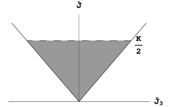
The $\operatorname{SU}(2)_{R}$ invariant $1/{16}$-BPS operators are built out of a ’closed fermi-surface’ model (see figure-2) described by the operator

$$\mathcal{J}{\kern-2.70004ptd}^{(K)}_{\text{closed}}\equiv\prod_{I=0}^{K}\prod_{m=0}^{I+1}\mathrm{Jdet}\left[(\bar{J}_{-})^{m}A^{(I)\,1}_{hw}\right]$$ (29)

where ’$\mathrm{Jdet}$’ stands for the anti-symmetrized multiplication of the entire $\operatorname{SU}(N)$ adjoint multiplet:

$$\mathrm{Jdet}\left[X\right]=\varepsilon_{a_{1}a_{2}\ldots a_{g}}X^{a_{1}}X^{a_{2}}\ldots X^{a_{g}}\hskip 10.00002pt,\hskip 10.00002ptX=\sum_{a=1}^{g}X^{a}T^{a}\quad\left(g=\dim G\right)\,,$$ (30)

for a fermionic X.

In a covariant form of (29) the left-handed angular momentum indices are totally symmetrized, whereas the action of $\bar{J}_{-}$ generates the multiplication of the entire $\operatorname{SU}(2)_{R}$ multiplet. This causes $\bar{J}$ to vanish. Thus, $\mathcal{J}{\kern-2.70004ptd}^{(K)}_{\text{closed}}$ belongs to the representation $[k,0,0]_{(J,0)}$ and carries two charges $(J,\,\mathcal{Q})$ which for large K and N equal:

$$J= (N^{2}-1)\sum_{I=0}^{K}\sum_{m=0}^{I+1}\frac{I}{2}=N^{2}\frac{K^{3}}{6}+O(K^{2},N)\,,$$ (31)

$$\mathcal{Q}=k= (N^{2}-1)\sum_{I=0}^{K}\sum_{m=0}^{I+1}1=N^{2}\frac{K^{2}}{2}+O(K,N)\,.$$ (32)

Solving for $K$, the scaling $J\sim\mathcal{Q}^{3/2}/N$ emerges, matching (9a).

The operator $\mathcal{J}{\kern-2.70004ptd}^{(K)}_{\text{closed}}$ is invariant under the chiral supercharge

$$[k,0,0]_{(J,0)}\xrightarrow{~{}Q~{}}[k+1,0,0]_{(J\pm\frac{1}{2},0)}\\ \Longleftrightarrow\quad\left[Q^{(i}_{\alpha},\mathcal{J}{\kern-2.70004ptd}^{(K)i_{1},\ldots i_{k})}_{\text{closed}}\right\}=0.$$ (33)

This originates from the Pauli exclusion principle as follows. The action of the supercharge ’splits’ each $A$ factor in $\mathcal{J}{\kern-2.70004ptd}^{(K)}_{\text{closed}}$ into two $A$ factors of smaller angular momentum (see (27b)). However, each of these factors already appears in $\mathcal{J}{\kern-2.70004ptd}^{(K)}_{\text{closed}}$. Thus $\big{[}Q^{1}_{\alpha},\mathcal{J}{\kern-2.70004ptd}^{(K)}_{\text{closed}}\big{\}}$ vanishes due to its fermionic nature. Using the highest-weight of $\operatorname{SU}(2)_{L}$ and $\operatorname{SU}(4)$ the construction can be viewed as a fermionic shell model, whose ’level’ is the left-handed angular momentum and the degeneracy is the $\operatorname{SU}(2)_{R}$ and $\operatorname{SU}(N)$ multiplet. In this picture, each $A$ factor is a creation operator of a fermionic state, and consequently, the $\mathcal{J}{\kern-2.70004ptd}^{(K)}_{\text{closed}}$ corresponds to filling all the shell up to level K. In terms of figure 2, for each level $\bar{J}$ (equally $J$) we fill all the $\operatorname{SU}(2)_{R}$ multiplet $\bar{J}^{3}=-\bar{J},\ldots\bar{J}$. The action of the chiral supercharge tries to split a fermion into two fermions belonging to lower levels, which is forbidden due to Pauli exclusion.

The case $\bar{J}=J$ :

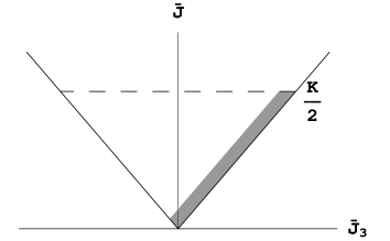
The equal left and right angular momenta $1/{16}$-BPS operators are built out of an ’open fermi-surface’ model (see figure-2) described by the operator

$$\mathcal{J}{\kern-2.70004ptd}^{(K)}_{\text{open}}\equiv\prod_{I=0}^{K}\mathrm{Jdet}\left[A^{(I)\,1}_{hw}\right]$$ (34)

The absence of $\bar{J}_{-}$ (compared to the closed shell model) in a covariant form causes all Lorentz indices (left and right handed) to be fully symmetrized. In terms of figure 2 at each level $\bar{J}$ (equally $J$) we occupy a single fermion with maximal $\bar{J}^{3}=\bar{J}$ . Calculating the charges in the large K and large N regime:

$$J=\bar{J}= (N^{2}-1)\sum_{I=0}^{K}\frac{I}{2}=N^{2}\frac{K^{2}}{4}+O(K^{2},N)\,,$$ (35)

$$\mathcal{Q}=k= (N^{2}-1)\sum_{I=0}^{K}1=N^{2}K+O(K,N)\,.$$ (36)

Once again, solving for $K$, the scaling $J=\bar{J}\sim\mathcal{Q}^{2}/N^{2}$ emerges, matching (10a).

Figure 1: The fermi sea picture of the close-shell operator

Figure 2: The fermi sea picture of the open-shell operator

The operators introduced for the fermi-surface models are manifestly descendants, as seen from the ”extra” supercharge in (33) and the failure to satisfy the BPS formula:

$$\Delta_{BPS}[k,0,0]_{(J,0)}=2+2J+\frac{3}{2}k\qquad\Delta[\mathcal{J}{\kern-2.70004ptd}^{(K)}]=2J+\frac{3}{2}k$$ (37)

In the rest of the section we show how to construct genuine $1/{16}$-BPS primaries by combining the fermi sea with bosonic operators. It is the addition of these bosonic excitations that yields a macroscopic entropy, i.e large enough degeneracy of operators, to generate a macroscopic black hole entropy in Planck units. There is also a large degeneracy of fermi surfaces as we will see in section 5.

4.1 Building $c^{1/4}$ Primaries

We are interested in modifying the shell construction to achieve several goals : saturation of the BPS bound, introduction of degeneracies (entropy) and having the operator be a primary. All these properties are satisfied by the addition of the adequate bosonic structures. In particular, we consider the following large family of $c^{1/4}$ operators :

$$\mathcal{O}^{(K,\vec{J})}\equiv\mathcal{J}{\kern-2.70004ptd}^{(K)}\left(C^{(K+1)}\mathcal{B}^{(\vec{J})}\right)_{GI}\qquad 2J_{i}\leq K$$ (38)

$\mathcal{J}{\kern-2.70004ptd}^{(K)}$ stands for either (29) or (34) and the subscript ’GI’ stands for a gauge invariant combination. $\vec{J}$ is a length $3L$ vector of angular momenta and

$$\mathcal{B}^{(\vec{J})}\equiv\prod_{i=1}^{L}B^{(2J_{i})\;12}B^{(2J_{L+i})\;13}B^{(2J_{2L+i})\;14}\,.$$ (39)

Notice that we are forced to add the bosons $B^{(I)1i}$ in triplets to have vanishing R-charges $p$ and $q$. The operator $C^{(K+1)}$ is the only building block in $\mathcal{O}^{(K,\vec{J})}$ satisfying $\Delta_{exc}=\Delta-2J-\frac{3}{2}k=2$ (all the rest has $\Delta_{exc}=0$). This suggests including a single excitation of type $C$ in each $c^{1/4}$ operator to saturate the BPS bound. As we explain below, the insertion of $C$ also plays a crucial role in allowing the full operator (38) to be a primary.

For the closed shells models the right-handed angular momentum coming from the $C^{(K+1)}$ and $\mathcal{B}^{(\vec{J})}$ is arbitrary. For the open shells model we need to symmetrize over all doted indices coming from the fermion and bosons resulting in $\bar{J}\simeq J$. Actually for the open shells one needs to work a little harder to create a primary. The total $\bar{J}$ is larger than $J$ due to the extra doted index of the Weyl spinors $\bar{\lambda}^{1}_{\dot{\alpha}}$, with the consequence that we are really describing a descendant operator. In section 5.2 we show how to fix this problem.

Acting with the chiral-supercharge (33) on the bosons $B^{(I)1i}$ and $C^{(K+1)}$ splits any boson into a sum of pairs consisting of a fermion and a boson in lower levels. All the fermions are of the type $A^{(I)1}$. Our operators are constructed in such a way that all $A^{(I)1}$ operators generated from the splitting of $B$ or $C$ are occupied. Hence $Q^{1}$ acting on $B$ or $C$ vanishes on the fermi surface (this is the origin of the constraints on the maximal $J_{i}$’s in (39)). The only exception is the supercharge acting on the $C^{(K+1)}$ which contains a term transforming it to a fermion in a higher level. Thus we are left with:

$$\left[Q^{(i}_{\alpha},\mathcal{O}^{(K,\bar{J})i_{1},\ldots i_{k})}\right\}=\mathcal{J}{\kern-2.70004ptd}^{(K)}\left(A^{(K+2)1}\mathcal{B}^{(\vec{J})}\right).$$ (40)

In term of charges

$$[k,0,0]_{(J,\bar{J})}\xrightarrow{~{}Q^{1}~{}}[k+1,0,0]_{(J+\frac{1}{2},\bar{J})}$$

The above argument proves that $\mathcal{O}^{(K,\bar{J})}$ obeys the semi-shortening condition of a super-multiplet with $[k+1,0,0]_{(J-\frac{1}{2},\bar{J})}$ removed. We are still left with the task of finding out when the operator $\mathcal{O}^{(K,\bar{J})}$ is a primary.

For the $\vec{J}=0$ case, we would like to suggest the following criteria for the bosonic part of the operator (although a full proof remains to be carried out). The constraint for $\mathcal{O}^{(K,\bar{0})}$ to be a primary is that its bosonic part (i.e, its $B$’s + a single $C$) is an $\mathcal{N}=4$ $1/{8}$-BPS operator, with the only difference being that a single $C^{(K+1)}$ is plugged into one of the traces.

The arguments for this claim are the following. The composite $\mathcal{O}^{(K,\vec{0})}$ is made out of three components:

1. The $B$’s part is a genuine $1/{8}$-BPS operator, annihilated only by $Q^{1}_{\alpha}$, and cannot be written as a $Q$, $\bar{Q}$ or a derivative of anything.

2. The $C^{(K+1)}$ part, which can be written as (no summation of repeated indices):

   $$C^{(K+1)}=\left(\{Q^{1},\bar{Q}_{1}\}\right)^{K+1}\cdot\{\bar{Q}_{i},[\bar{Q}_{j}\bar{M}^{ij}]\}$$

3. The closed shells operator $\mathcal{J}{\kern-2.70004ptd}^{(K)}$

We argue that any attempt to write $\mathcal{O}^{(K,\vec{0})}$ as a $Q$ or a $\bar{Q}$ of another operator, just by ”pulling out” a single supercharge fails. Our arguments are not complete, but we analyse the simplest ways to write $\mathcal{O}^{(K,\vec{J})}$ as a $Q$ or $\bar{Q}$ of another operator.

First we try ”pulling out” a supercharge from one of the components. We cannot pull out anything from the $B$’s part, so we try to write:

$$\mathcal{O}^{(K,\vec{0})}=Q\cdot\left(\mathcal{J}{\kern-2.70004ptd}^{(K)}Y\mathcal{B}^{(\vec{0})}\right)\qquad\text{or}\qquad\mathcal{O}^{(K,\vec{0})}=Q\cdot\left(XC^{(K+1)}\mathcal{B}^{(\vec{0})}\right)$$ (41)

For the above to ”work” we need $Q$ to annihilate $\mathcal{B}^{(\vec{0})}$, the only possible supercharges are $Q^{1}_{\alpha}$. Considering the supersymmetry transformation, we see that $X$ and $Y$ in (41) are:

$$C^{(K+1)}= \,Q^{1}_{+1/2}\cdot A^{(K)1} \Rightarrow Y= \,A^{(K)1}$$

$$\mathcal{J}{\kern-2.70004ptd}^{(K)}= \,Q^{1}_{-1/2}\cdot\frac{\partial^{2}\mathcal{J}{\kern-2.70004ptd}^{(K)}}{\partial A^{(I)1}A^{(I^{\prime})1}}A^{(I+I^{\prime}+1)1} \Rightarrow X= \,\frac{\partial^{2}\mathcal{J}{\kern-2.70004ptd}^{(K)}}{\partial A^{(I)1}A^{(I^{\prime})1}}A^{(I+I^{\prime}+1)1}.$$

In the above expression, a derivative of a composite with respect to fermionic operators should be understood as removing a single copy of the operator from the composite.

The first option fails, due to Pauli exclusion - the operator Y is annihilated on the fermi sea. The second option inserts holes in the fermi sea at $A^{(I)1}$ and $A^{(I^{\prime})1}$. This means that the variation has extra terms coming from the variation of $C^{(K+1)}$ which fills one of these holes. Hence, we do not obtain equation (41) in this way. It does not seem possible to cancel these extra terms (for example, by taking sums over different $I$ and $I^{\prime}$), although a full proof remains to be formulated.

The next possibility we attempt to falsify is ”pulling out” a supercharge from the combination of the fermi-sea and bosons $\mathcal{B}^{(\vec{0})}$, i.e splitting a boson into a pair of a fermion and a boson:

$$\mathcal{O}^{(K,\vec{0})}=Q\cdot\left(\frac{\partial\mathcal{J}{\kern-2.70004ptd}^{(K)}}{\partial A^{(I)1}}C^{(K+1)}\frac{\partial\mathcal{B}^{(\vec{0})}}{\partial B^{(0)1i}}B^{(I+1){i^{\prime}j^{\prime}}}\right)$$

Checking the supersymmetry transformations, we see that the only possibility is having $i^{\prime}j^{\prime}=1i$ and $Q=Q^{1}_{-1/2}$. Now we can repeat the argument that the hole in the fermi-sea allows for non-vanishing transformation of the $C^{(K+1)}$ and fails to achieve the above equality.

Trying to ”pull out” a supercharge form the combination of the $C^{(K+1)}$ and $\mathcal{B}^{(\vec{0})}$, fails from similar reasonings. We are left to check that we cannot ”pull out” a supercharge from the combination of the fermi-sea and the $C^{(K+1)}$. To examine this option, consider the supersymmetry transformation:

$$Q^{1}_{-\frac{1}{2}}\cdot\left(\frac{\partial\mathcal{J}{\kern-2.70004ptd}^{(K)}}{\partial A^{(I)1}}C^{(J+I+1)}\mathcal{B}^{\vec{(}0)}\right)=\\ =\mathcal{J}{\kern-2.70004ptd}^{(K)}\,C^{(J)}\mathcal{B}^{(\vec{0})}+\sum_{r=K+2}^{J+I+1}\frac{\partial\mathcal{J}{\kern-2.70004ptd}^{(K)}}{\partial A^{(I)1}}A^{(r-1)1}C^{(J+I+1-r)}\mathcal{B}^{(\vec{0})}$$ (42)

We would like to know for what values of $J$, the sum in the rhs will be non-zero for any value of I ($I\leq K$). In addition for $\mathcal{J}{\kern-2.70004ptd}^{(K)}\,C^{(J)}\mathcal{B}^{(\vec{0})}$ to be BPS we must have  $J<K+2$. The conditions that $J<K+2$ and that $J+I+1\geq K+2$ for all $0\leq I\leq K$ have a unique solution of $J=K+1$, which is the operator that we presented before.

From the above discussion we also learn the existence of a general rule: in order to construct a primary from a fermionic shell model, we must have a $C$ factor in an empty shell adjacent to the last filled shell.

4.2 Charges

$\mathcal{O}^{(K,\bar{J})}_{\text{closed}}$ and $\mathcal{O}^{(K,\bar{J})}_{\text{open}}$ are constructed so that the $\operatorname{SU}(2)_{L}$ and $\operatorname{SU}(4)$ charges are additive. The contributions of each composite to the global charges carried by the operator are summarized in table-3.

	$J$	$~{}~{}~{}(k,p,q)~{}~{}~{}$	$\Delta$	$~{}~{}\Delta-2J-\frac{3}{2}k$
$A^{(I),1}$	$I/2$	$(1,0,0)$	$I+3/2$	$0$
$B^{(I)12}$	$I/2$	$(0,1,0)$	$I+1$	$1$
$B^{(I)13}$	$I/2$	$(1,-1,1)$	$I+1$	$-1/2$
$B^{(I)14}$	$I/2$	$(1,0,-1)$	$I+1$	$-1/2$
$C^{(I)}$	$I/2$	$(0,0,0)$	$I+2$	$2$

Table 3: Charges of $\mathcal{J}{\kern-2.70004ptd}^{(K,\vec{J})}$ building blocks.

Remembering that the $B$’s come in triplets $B^{12}B^{13}B^{14}$, we immediately see the emergence of the BPS formula:

$$\Delta=2+2J+\frac{3}{2}k\,.$$ (43)

We calculate the charges of the closed shell model with $B$’s, postponing the open shell model discussion to section 5.2. For the closed shells model, the total charges are computed by summing the contributions over the different ingredients:

$$J= (N^{2}-1)\sum_{I=0}^{K}\sum_{m=0}^{I+1}\frac{I}{2}+\frac{K+1}{2}+\sum_{i=1}^{3L}J_{i}$$ (44a)

$$\mathcal{Q}=k= (N^{2}-1)\sum_{I=0}^{K}\sum_{m=0}^{I+1}1+2L$$ (44b)

The right handed angular momentum is bounded from above by $\sum_{i=1}^{3L}J_{i}$, but could be taken to $0$ by suitable contractions.

Taking the large R-charge and large angular momentum limit is equivalent to taking $K\gg 1$. Simplifying the charges in this case and taking $N\gg 1$:

$$J\approx N^{2}\frac{K^{3}}{6}+\sum_{i=1}^{3L}J_{i}\leq N^{2}\frac{K^{3}}{6}+\frac{3}{2}LK\,,$$ (45a)

$$\mathcal{Q}\approx N^{2}\frac{K^{2}}{2}+2L\,,$$ (45b)

where the bound in (45a) originates from (38). The maximal value for $J$ in this family of operators is obtained as follows. First, we solve (45b) for L and substitute it back into (45a)

$$J\leq\frac{3\mathcal{Q}}{4}K-\frac{5}{24}N^{2}K^{3}\,.$$ (46)

If we view the rhs as a function of K, the latter is bounded from above. This generates an upper bound for $J$ for all $\mathcal{Q}$ given by

$$\frac{J_{max}}{N^{2}}=\frac{\sqrt{3}}{\sqrt{20}}{\sqrt{2}}\left(\frac{\mathcal{Q}}{N^{2}}\right)^{3/2}\approx 0.39\,{\sqrt{2}}\left(\frac{\mathcal{Q}}{N^{2}}\right)^{3/2}$$ (47)

If we compare this result to the supergravity scaling (9a) (with $\gamma=0$), we realize that our fermi-sea operators reproduce the same scaling relation, but differ in an order one number in its coefficient. In particular, the angular momentum is approximately $0.39$ times smaller than the supergravity charge. If we had neglected the bosons, we would have found :

$$\frac{J}{N^{2}}=\frac{\sqrt{2}}{3}\left(\frac{\mathcal{Q}}{N^{2}}\right)^{3/2}$$

Thus, the addition of the bosons improves the order 1 coefficient but not enough to match the supergravity result.

One can also wonder about lower values of $J$. Naively one can add many bosons in low angular momentum levels. Such operators have angular momentum linear in the charge (or less). For example, adding bosons up to level $K^{\prime}$ which is fixed as $K$ scales to infinity, pulls down the angular momentum to charge scaling down to $J\sim\mathcal{Q}^{\beta}$ ($0\leq\beta<3/2$). However, the degeneracy of such configuration is of the same order as the degeneracy of standard $1/{8}$-BPS operators which scales as $N\log N$ [17]. As we discuss in the following section, the entropy of our operators, with large angular momentum ($J\sim\mathcal{Q}^{3/2}/N$), scales as $\mathcal{Q}$ (which is much greater than $\gg N^{2}$). Thus operators with scaling $\beta<3/2$ are subdominant and should not affect the macroscopical features of the ensemble.

The shell structure that we discussed, and its completion to primary operators, reproduces the scaling relation $J(\mathcal{Q})$ up to numerical coefficient. We now present a simple computation that reproduces the correct scaling of the entropy as well, up to order 1 coefficient. We carry out the computation both for the open and closed shells. In both cases, the entropy will be proportional to $\mathcal{Q}$, which is the correct result, but we will see that it comes about in different ways for the two cases.

4.2.1 Entropy of the Closed Shell Model

In this section we estimate the degeneracy of the bosonic part under the following assumptions :

• Ignoring the constraints for the operator to be primary.

• Ignoring any finite $N$ dependence.

The statistical model we use is a Fock space of free bosons. The single particle bosonic states contribution to the degeneracy are: $B^{(I)12}$, $B^{(I)13}$ and $B^{(I)14}$, with I taking values from $0$ to $K$. We introduce a chemical potential for the right-handed angular momentum ($J$) and for the R-charges ($k$, $p$ and $q$) allowing for $\bar{J}$ to be determined by the ensemble average. The partition function takes the familiar form (see [19]) of summation over all multi-particle states:

$$\log Z=\sum_{r=1}^{\infty}\frac{1}{r}f_{sp}(r\gamma_{1}\,,\,r\gamma_{2}\,,\,r\gamma_{3}\,,\,r\mu)\hskip 10.00002pt,\hskip 10.00002pt$$ (48)

with the single particle partition function:

$$f_{sp}(\gamma_{1}\,,\,\gamma_{2}\,,\,\gamma_{3}\,,\,\mu)=\sum_{I=0}^{K}\sum_{a=1}^{N^{2}-1}\sum_{m=0}^{I}\left(e^{\gamma_{1}-\gamma_{3}}+e^{\gamma_{1}-\gamma_{2}+\gamma_{3}}+e^{\gamma_{2}}\right)e^{\frac{\mu I}{2}}$$ (49)

The chemical potentials are defined such that the boson contribution to the charges is :

$$\hat{k}=\frac{\partial\log Z}{\partial\gamma_{1}}\,,\qquad\hat{p}=\frac{\partial\log Z}{\partial\gamma_{2}}\,,\qquad\hat{q}=\frac{\partial\log Z}{\partial\gamma_{3}}\,,\qquad\hat{J}=\frac{\partial\log Z}{\partial\mu}\,.$$ (50)

We are interested in $p=q=0$, which determines :

$$\gamma_{1}=3\gamma_{3}=\frac{3}{2}\gamma_{2}\equiv\gamma$$ (51)

Evaluating the partition function (in the large $N$ and $K$ limit):

$$\log Z(\mu,\gamma)= -3N^{2}\sum_{I=0}^{K}(I+1)\log\left[1-\exp\left(\frac{2}{3}\gamma+\frac{\mu}{2}I\right)\right]=$$ (52)

$$\approx -3N^{2}K^{2}\int_{0}^{1}dy\,y\log\left[1-\exp\left(\frac{2}{3}\gamma+\frac{\mu}{2}yK\right)\right]=$$ (53)

$$= \frac{12K^{2}N^{2}}{(K\mu)^{2}}\left(Pl\left[3,\,e^{\frac{2}{3}\gamma}\right]-Pl\left[3,\,e^{\frac{2}{3}\gamma+\frac{K\mu}{2}}\right]+\frac{K\mu}{2}Pl\left[2,\,e^{\frac{2}{3}\gamma+\frac{K\mu}{2}}\right]\right)$$ (54)

where $Pl\left[n,\,z\right]$ is the PolyLog function. The form of the partition function suggests using the variables:

$$x=\frac{K\mu}{2}\hskip 10.00002pt,\hskip 10.00002pt\xi=e^{\frac{2}{3}\gamma}$$

We wish to set the chemical potentials to fix the charges (remembering the contribution of the fermions):

$$J= \frac{N^{2}K^{3}}{6}+\hat{J}=\frac{N^{2}K^{3}}{6}+\frac{K}{2}\frac{\partial\log Z}{\partial x}=N^{2}K^{3}\,a(x,\xi)$$ (56)

$$\mathcal{Q}= \frac{N^{2}K^{2}}{2}+\hat{k}=\frac{N^{2}K^{2}}{2}+\frac{2}{3}\frac{\partial\log Z}{\partial\log\xi}=N^{2}K^{2}\,b(x,\xi)$$ (57)

with,

$$a(x,\xi)\equiv \,\frac{1}{6}-\frac{3}{2x}\log\left(1-\xi e^{x}\right)-\frac{3}{x^{3}}\left(Pl\left[3,\,\xi\right]-Pl\left[3,\,\xi e^{x}\right]+xPl\left[2,\,\xi e^{x}\right]\right)$$ (58)

$$b(x,\xi)\equiv \,\frac{1}{2}-\frac{2}{x}\log\left(1-\xi e^{x}\right)+\frac{2}{x^{2}}\left(Pl\left[2,\,\xi\right]-Pl\left[3,\,\xi e^{x}\right]\right)$$ (59)

There are two conditions that we would like to force on the ensemble:

$$\frac{J}{N^{2}}={\alpha}{\sqrt{2}}\left(\frac{\mathcal{Q}}{N^{2}}\right)^{3/2}\hskip 10.00002pt,\hskip 10.00002ptJ\gg\mathcal{Q}$$ (60)

The first is the supergravity scaling (from the previous discussion we expect $\alpha$ to be of order 1). The second is the condition for the energy to be dominated by the angular momentum. Applying (56) to (60) we conclude:

$$a\sim b^{3/2}\hskip 10.00002pt,\hskip 10.00002ptK\gg\frac{b}{a}\sim b^{-1/2}$$

The interesting regime is $K$ large, $a$,$b$ fixed ($x$, $\xi$ fixed). In this regime the scaling of the entropy becomes :

$$S(J,\mathcal{Q})= \,\log Z-\frac{2}{3}\gamma\cdot\hat{k}-\frac{\mu}{2}\cdot\hat{J}=K^{2}N^{2}f(x,\xi)$$ (61)

$$\sim \,K^{2}N^{2}\sim\,\mathcal{Q}$$ (62)

Since the variable $x$ and $\xi$ depend on $\mathcal{Q}$ and $J$ in such a manner that they do not scale with $K$ or $N$, therefore the function $f(x,\xi)$ does not scale with $K$ or $N$.

This result matches qualitatively the supergravity relation (9b) and confirms our claim that the $1/{16}$-BPS operators constructed from the closed shell models indeed carry macroscopical large entropy ($S\sim N^{2}K^{2}$) unlike the $1/{8}$-BPS operators with no angular momentum ($S\sim N\log N$).

In the above calculation we used a slightly different scheme than in the rest of the paper. We fixed $J$ and $\mathcal{Q}$ and let $\bar{J}$ be determined by the ensemble (instead of fixing $\bar{J}$ and $\mathcal{Q}$). This was done for convenience and it should not affect the validity of our conclusion.

4.2.2 Entropy of the Open Shells Models

The calculation for the open shells is done in a similar spirit to the closed shells one with the summation over the $\operatorname{SU}(2)_{R}$ multiplet removed.

$$\log Z=\sum_{r=1}^{\infty}\frac{1}{r}f_{sp}(r\gamma\,,\,r\mu)\hskip 10.00002pt,\hskip 10.00002ptf_{sp}(\gamma\,,\,\mu)=\sum_{I=0}^{K}\sum_{a=1}^{N^{2}-1}3e^{\frac{2}{3}\gamma+\frac{\mu I}{2}}$$ (63)

Repeating the steps of the previous subsection, we obtain :

$$J= \frac{N^{2}K^{2}}{4}+\hat{J}=N^{2}K^{2}\,a(x,\xi)$$ (64)

$$\mathcal{Q}= N^{2}K+\hat{k}=N^{2}K\,b(x,\xi)$$ (65)

with,

$$a(x,\xi)\equiv \,\frac{1}{4}-\frac{3}{2x}\log\left(1-\xi e^{x}\right)-\frac{3}{2x^{2}}\left(Pl\left[2,\,\xi e^{x}\right]-xPl\left[2,\,\xi\right]\right)$$ (66)

$$b(x,\xi)\equiv \,1-\frac{2}{x}\left(\log\left(1-\xi e^{x}\right)-\log\left(1-\xi\right)\right)$$ (67)

The two conditions that we force on the ensemble are :

$$\frac{J}{N^{2}}=\alpha\left(\frac{\mathcal{Q}}{N^{2}}\right)^{2}\hskip 10.00002pt,\hskip 10.00002ptJ\gg\mathcal{Q}\hskip 10.00002pt\Rightarrow\hskip 10.00002pta\sim b^{2}\hskip 10.00002pt,\hskip 10.00002ptK\gg b^{-1}$$ (68)

We find that $a(x,\xi)$ and $b(x,\xi)$, cannot scale with $K$ or $N$. In general, solving (64) for $x$ and $\xi$, we conclude that all the dependence on $\mathcal{Q}$ and $J$ is such that they are order 1 numbers (not scaling with $K$ or $N$). Thus, the entropy of the ensemble is given by :

$$S(J,\mathcal{Q})= \,\log Z-\frac{2}{3}\gamma\cdot\hat{k}-\frac{\mu}{2}\cdot\hat{J}=K^{2}Nf(x,\xi)$$ (69)

$$\sim \,K^{2}N\sim\,\mathcal{Q}$$ (70)

The result matches qualitatively the supergravity relation (10b) and matches our expectations that the $1/{16}$-BPS operators constructed from the open shell models indeed carry macroscopical large entropy ($S\sim N^{2}K$).

5 Generalizations

In this section, we take some steps towards generalizing the structures studied before. Even though one can potentially achieve this by adding more fields to the operators in question, we focus here on a more interesting possibility which is the deformation of the fermi sea structure. We will not describe the bosonic part of the operator nor discuss whether these new operators are primary or not.

First of all, we provide the basic rules that any shell has to satisfy. A fermion in the fermi-sea is characterized by its quantum numbers under $\operatorname{SU}(2)_{L}\times SU(2)_{R}$, i.e.  $A_{\left|J,\,m=J\right\rangle\left|\bar{J}=J+1/2,\,\bar{m}\right\rangle}$. Under the action of the supercharge (16), the fermion splits according to :

$$A_{\left|J,J\right\rangle\left|J+\frac{1}{2},\,\bar{m}\right\rangle}\xrightarrow{Q^{1}_{-1/2}}\sum_{\begin{subarray}{c}J_{1},J_{2}\\ \bar{m}_{1},\bar{m}_{2}\end{subarray}}A_{\left|J_{1},J_{1}\right\rangle\left|J_{1}+\frac{1}{2},\,\bar{m}_{1}\right\rangle}\otimes A_{\left|J_{2},J_{2}\right\rangle\left|J_{2}+\frac{1}{2},\,\bar{m}_{2}\right\rangle}$$ (71)

$$\text{with,}\qquad J=J_{1}+J_{2}+1/2\hskip 10.00002pt,\hskip 10.00002pt\bar{m}=\bar{m}_{1}+\bar{m}_{2}$$ (72)

Denoting the set of occupied fermions by ${\mathcal{M}}$, the conditions for invariance under (16) are that  $A_{\left|J_{1},J_{1}\right\rangle\left|J_{1}+\frac{1}{2},\,\bar{m}_{1}\right\rangle}\in\mathcal{M}$ or, $A_{\left|J_{2},J_{2}\right\rangle\left|J_{2}+\frac{1}{2},\,\bar{m}_{2}\right\rangle}\in\mathcal{M}$ for each possible combination in the sum (72).

Figures 4 and 4 exhibit two methods of finding a set ${\mathcal{M}}$ satisfying these constraints (there are also ways of combining the two methods). In section 5.1 we discuss the method corresponding to 4, and in section 5.2 we discuss the generalization corresponding to 4.

Figure 3: A band of closed-shells

Figure 4: A general fermi sea picture

5.1 Fermionic Bands

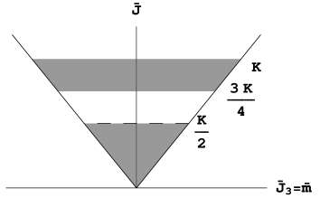
The first generalization that we describe is to add fermions in a level higher than $K$. Any fermionic operator $A^{(I)\,1}$ with level up to $2K$ splits under the supercharge $Q^{1}$ action into two fermions, such that at least one of them is below level $K$. Hence, such action is annihilated on the closed shell. We can continue this construction by adding closed shells near level $2K$ (we call this a band) allowing to have fermions with level up to $3K$.

Iterating this procedure, we can build multiple fermionic bands. Leaving the details to appendix-B, we search for the best configuration of fermions in $n$ bands. The upper bound on the angular momentum to charge ratio is found for the single-band case drawn in figure-4, with:

$$J=\alpha{N^{2}}{\sqrt{2}}\left(\frac{\mathcal{Q}}{N^{2}}\right)^{3/2}\hskip 20.00003pt,\hskip 20.00003pt\alpha\leq\frac{3}{2\sqrt{11}}\approx 0.45.$$ (73)

The bound is saturated when the contribution of the bosons is completely negligible.

5.2 General Fermionic Shells

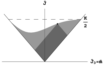
As with any fermi surface, we can deform it. For our surface in the ${\bar{J}}-{\bar{m}}$ plane, this can be done as follows. Regarding $(\bar{J},\bar{m})$ as a 2-vector, we see that the splitting of a fermion in (72) by the supercharges results in a 2-vector summation:

$$(\bar{J},\bar{m})=(\bar{J}_{1},\bar{m}_{1})+(\bar{J}_{2},\bar{m}_{2})\hskip 20.00003pt,\hskip 20.00003pt\bar{J}_{i}\geq\left|\bar{m}_{i}\right|\quad(i=1,2)\,,$$

where the last inequality is the condition that the vector represents true $\operatorname{SU}(2)_{R}$ quantum numbers. Therefore a fermion can only split into parts that are confined to a rectangular whose opposite corners are the original vector and the origin (described in figure 4 by the darker part of the fermi-sea).

Hence, the description of the fermi-sea is given by the contour of the last (highest angular momentum) occupied fermions $\bar{J}_{max}(\bar{m})$. The condition for invariance under the supercharge is simply:

$$\left|\frac{d\bar{J}_{max}}{dm}\right|\leq 1$$

Even though the calculation of charges of the surface is somewhat complicated, the value of $\mathcal{Q}$ , $J$ and $\bar{J}^{3}$ are just integrals (in the large $K$ limit) over the fermi-sea:

$$\frac{J}{N^{2}}= \iint_{sea}d\bar{J}d\bar{m}\,\bar{J}$$ (74a)

$$\frac{\mathcal{Q}}{N^{2}}= \iint_{sea}d\bar{J}d\bar{m}\,1$$ (74b)

$$\frac{\bar{J}^{3}}{N^{2}}= \iint_{sea}d\bar{J}d\bar{m}\,\bar{m}$$ (74c)

For (74a) recall that we have chosen a highest weight with respect to $\operatorname{SU}(2)_{L}$ (see eq. 28). A state constructed this way has a well defined $\bar{J}^{3}$ eigenvalue, but one still needs to project to states with specific $\bar{J}$.

In the following paragraph we describe in detail an example for a class of fermi surfaces where we have a good control over all charges. The operators in this class have the nice feature that they have scalings matching the black holes with arbitrary $J$ and $\bar{J}$.

5.2.1 Generalized open-shells

The fermi sea we will describe is a generalization of the open-shell model, where a constant number of fermions at each level is kept. The corresponding fermi-sea is drawn in figure-5.

Figure 5: Fermi sea of generalized open-shells

In order to construct these operators, we need to be more explicit with the $\operatorname{SU}(2)_{R}$ symmetry. First, rewrite the closed shell operator in a manifestly covariant form:

$$\mathcal{J}{\kern-2.70004ptd}^{(K)}_{\text{closed}}\equiv\prod_{I=0}^{K}\prod_{m=0}^{I+1}\mathrm{Jdet}\left[(\bar{J}_{-})^{m}A^{(I)1}\right]=\prod_{I=0}^{K}\mathrm{Jdet}\left[\mathcal{A}{\kern-1.79993ptd}^{(I,I+1)}\right]$$ (75)

where,

$$\mathcal{A}{\kern-1.79993ptd}^{(I,I+1)}=\prod_{m=0}^{I+1}(\bar{J}_{-})^{m}A^{(I)1}\equiv ~{}\left(A^{(I)1}_{(\alpha_{1}\cdots\alpha_{I})(\dot{\alpha}_{1}\cdots\dot{\alpha}_{I+1})}\right)\cdot\left(A^{(I)1}_{(\beta_{1}\cdots\beta_{I})(\dot{\beta}_{1}\cdots\dot{\beta}_{I+1})}\epsilon^{\dot{\beta}_{I+1}\dot{\alpha}_{I+1}}\right)\cdot$$ (76)

$$\quad\cdots\left(A^{(I)1}_{(\omega_{1}\cdots\omega_{I})(\dot{\omega}_{1}\cdots\dot{\omega}_{I+1})}\epsilon^{\dot{\omega}_{I+1}\dot{\alpha}_{1}}\epsilon^{\dot{\omega}_{I}\dot{\beta}_{1}}\epsilon^{\dot{\omega}_{I-1}\dot{\gamma}_{1}}\cdots\right)$$ (77)

with all undoted indices symmetrized.

The above operator can be generalized by stopping the multiplication before all $\operatorname{SU}(2)_{R}$ indices are exhausted:

$$\mathcal{A}{\kern-1.79993ptd}^{(I,\bar{I})}=\prod_{m=0}^{\bar{I}}(\bar{J}_{-})^{m}A^{(I)1} \equiv~{}\left(A^{(I)1}_{(\alpha_{1}\cdots\alpha_{I})(\dot{\alpha}_{1}\cdots\dot{\alpha}_{I+1})}\right)\cdot\left(A^{(I)1}_{(\beta_{1}\cdots\beta_{I})(\dot{\beta}_{1}\cdots\dot{\beta}_{I+1})}\epsilon^{\dot{\beta}_{I+1}\dot{\alpha}_{I+1}}\right)\cdot$$ (78)

$$\cdots\left(A^{(I)1}_{(\chi_{1}\cdots\chi_{I})(\dot{\chi}_{1}\cdots\dot{\chi}_{I+1})}\epsilon^{\dot{\chi}_{I+1}\dot{\alpha}_{I+2-\bar{I}}}\epsilon^{\dot{\chi}_{I}\dot{\beta}_{I+2-\bar{I}}}\epsilon^{\dot{\chi}_{I-1}\dot{\gamma}_{I+2-\bar{I}}}\cdots\right)$$ (79)

with all uncontracted indices of the same type (doted and undoted) symmetrized. The operator has exactly $(1+\bar{I})$ fermions, independently of the level I.

We define the generalized open shells as :

$$\prod_{I=0}^{K^{\prime}-1}\mathrm{Jdet}\left[\mathcal{A}{\kern-1.79993ptd}^{(I,I+1)}\right]\prod_{I=K^{\prime}}^{K}\mathrm{Jdet}\left[\mathcal{A}{\kern-1.79993ptd}^{(I,K^{\prime})}\right]\left(C^{(K+1)}\mathcal{B}^{(\vec{J})}\right)_{GI}$$ (80)

This operator will be BPS if the contractions of the $\operatorname{SU}(2)_{R}$ indices of the $B$’s are limited in a similar fashion to the fermions (i.e, $\bar{J}-\bar{J}^{3}$ of each $B$ smaller than $K^{\prime}/2$). Taking $K^{\prime}=\beta K$, the charges of the operator (for simplicity ignoring the contribution from the bosons) are:

$$\frac{2J}{N^{2}}\approx\sum_{I=0}^{\beta K-1}I^{2}+\sum_{I=\beta K}^{K}I(\beta K+1)\approx\frac{\beta}{2}\left(1-\frac{\beta^{2}}{3}\right)K^{3}$$ (81)

$$\frac{2\bar{J}}{N^{2}}\approx\sum_{I=\beta K}^{K}(I+1-\beta K)(\beta K+1)\approx\frac{\beta}{2}(1-\beta)^{2}K^{3}$$ (82)

$$\frac{\mathcal{Q}}{N^{2}}\approx\sum_{I=0}^{\beta K-1}I+\sum_{I=\beta K}^{K}(\beta K+1)\approx\beta\left(1-\frac{\beta}{2}\right)K^{2}$$ (83)

Solving for K, we find,

$$J=\frac{1}{\gamma(\beta)}\bar{J}=\alpha(\beta)\frac{N^{2}\sqrt{2}}{\sqrt{1-\gamma(\beta)^{2}}}\left(\frac{\mathcal{Q}}{N^{2}}\right)^{3/2}\,,$$ (84)

with,

$$\gamma(\beta)=\frac{(1-\beta)^{2}}{1-\frac{\beta^{2}}{3}}\,,$$ (85)

$$\alpha(\beta)=\frac{\sqrt{\left(1-\frac{2}{3}\beta\right)\left(1-\beta+\frac{\beta^{2}}{3}\right)}}{(2-\beta)^{3/2}}\,.$$ (86)

In the allowed range $\beta\in[0,1]$, the ratio $\alpha(\beta)$ is bounded by $\frac{1}{2\sqrt{2}}$, which again is smaller than the supergravity result (9a).

The shell construction has an interesting scaling property if we take a small $K^{\prime}=M$ not scaling with K, i.e all shells are almost empty. The charges of the operator (for simplicity ignoring contribution form the B’s) are:

$$\frac{2J}{N^{2}}\approx\sum_{I=0}^{M-1}I^{2}+\sum_{I=M}^{K}(M+1)I\approx(M+1)\frac{K^{2}}{2}$$ (87a)

$$\frac{2\bar{J}}{N^{2}}\approx\sum_{I=M}^{K}(I+1-M)(M+1)\approx(M+1)\frac{K^{2}}{2}-K(M^{2}-1)$$ (87b)

$$\frac{\mathcal{Q}}{N^{2}}\approx\sum_{I=0}^{M-1}I+\sum_{I=M}^{K}(M+1)\approx(M+1)K$$ (87c)

And the ratios are:

$$J=\frac{2}{5-b}\,\frac{N^{2}(1-b)}{4}\left(\frac{\mathcal{Q}}{N^{2}}\right)^{2}\hskip 20.00003pt,\hskip 20.00003ptJ-\bar{J}=\frac{1+3b}{4(1-b)}\mathcal{Q}$$ (88)

with $b=\frac{2M-3}{2M+1}$  defined so that the $J-\bar{J}$ equation matches the supergravity result (11). This result has the asymptotic behavior of the black holes with $J=\bar{J}$, missing the supergravity ratio (10a) by a factor $~{}\frac{2}{(5-b)}\leq\frac{1}{2}$. The open fermi surface described in section-4, is the $M=0$ case.

6 Summary and Outlook

In this paper, we used the $\mathcal{N}=4$ field theory at weak non-zero coupling to reproduce the relations $J(Q)$ in $1/{16}$-BPS black holes in $AdS_{5}\times S^{5}$ in the regimes (9a) and (10a). The main ingredient in our construction is the filling of fermi surfaces which is used to cancel the supersymmetry variation of the operator $(D_{\alpha\dot{\alpha}})^{n}$. We expect the fermi sea to play an important role in the microscopic description of any $1/{16}$-BPS AdS₅ black holes in the limit of large $J$ and ${\bar{J}}$ (since the CFT operators will contain many covariant derivatives). It would be interesting to study the 3-charge generalization of our discussion, and in particular, to understand how the complicated angular momentum and R-charges relations in supergravity appear from the field theory dual for this cases.

We have used only a subset of the allowed fields and shell configurations. It is therefore not very surprising that we did not find the exact $J(Q)$ or $S(Q)$ of the operators as computed in [9]. We expect that the latter also uses the fermionic shell structure that we discussed here. If our operators are indeed primary, as we conjecture, our results suggest the existence of new $1/{16}$-BPS black objects in $AdS_{5}\times S^{5}$.

There are two lines of generalizations that one can consider. In this work, we have mostly focused on two specific filling of shells - one in which the full ${\bar{J}}$ multiplet is filled, and one in which only states with near to maximal ${\bar{J}}_{3}$ are filled. We briefly mentioned other possibilities. Clearly there is a rich variety of allowed fillings and the classification of all possible $J(Q)$ relations will be carried elsewhere [23].

For example, consider a fermi sea constructed from two regions as depicted in figure 6. Region A in which full ${\bar{J}}$ multiplets are filled up to some ${\bar{J}}_{0}=K^{\prime}/2$ (i.e., up to $\sim K^{\prime}$ derivatives). In region B, from angular momentum $\frac{K^{\prime}+1}{2}$ up to some ${\bar{J}}_{1}=K/2$ where we fill states with ${\bar{m}}={\bar{J}}$ and ${\bar{m}}=-{\bar{J}}$. This state can be projected to a ${\bar{J}}=0$ state. This configuration interpolates between the relation $J/N^{2}\propto(\mathcal{Q}/N^{2})^{3/2}$ for ${\bar{J}}_{1}-{\bar{J}}_{0}\ll{\bar{J}}_{0}$ (no region B) and $J/N^{2}\propto(\mathcal{Q}/N^{2})^{2}$ for ${\bar{J}}_{0}\ll{\bar{J}}_{1}$ (no region A). Of course, since we have not exhibited a full supersymmetric completion of this specific mixture of shell filling, we do not know for sure that such an operator exists, but we find it very plausible.

Figure 6: Fermi sea of 2 two regions model.

The interpretation of this state in $AdS_{5}$ is also unclear. The two regions $B$, if continued all the way down to ${\bar{J}}=0$ correspond to two black holes with ${\bar{J}}=J$ but with opposite ${\bar{J}}_{3}$. Region A, if taken by itself, might correspond to a single black hole with ${\bar{J}}=0$. What does the full configuration correspond to ? Does it correspond to highly deformed black holes, in which the angular momenta ${\bar{J}}_{3}$ is distributed non-uniformly in space ? We believe this to be the case, although more work is needed to verify this picture [23], but it is clear that we have not exhausted the full range of possible $J(Q)$ and $S(Q)$ scalings, nor space-time morphologies of the black holes.

The second possible generalization involves adding more types of fields. A set of attractive candidates are the field strength operators $F_{\alpha\beta}$ and theirs derivatives ($G^{(I+2)}$’s). These operators carry no R-charges. Thus they are excellent candidates to improve the angular momentum to R-charge ratio reported in this paper. A BPS combination probably involves the addition of chiral fermions $\lambda_{\alpha i}$ needed to cancel the $F_{\alpha\beta}$’s supersymmetry transformations. More precisely, acting with $Q^{1}$ on $D.....DF$ generates $A$’s from variations of the covariant derivatives, for which we need shells as we discussed so far, and $D....D[\lambda_{i\alpha},M^{1i}]$. Including the latter in the operator from the start means that the SUSY variation of $D....DF$ will be zero within this operator (the $Q^{1}$ variation of $[\lambda_{i\alpha},M^{1i}]$ is zero). It is interesting to point out the existence of supersymmetric $AdS_{5}\times S^{5}$ configurations having angular momentum but no R-charge [24]. The existence of this type of operators, which is left to future work, could provide evidence for the existence of these spacetimes in string theory, since the existence of a naked singularity of the latter render their interpretation unclear.

7 Acknowledgments

We would like to thank O. Aharony, Y. Antebi, D.Kutasov, F. Larsen and S.Minwalla for useful discussions and comments. JS would like to thank the Weizmann Institute of Science for hospitality during different periods in the completion of this work. The work of MB is supported by the Israel Science Foundation, by the Braun-Roger-Siegl foundation, by EU-HPRN-CT-2000-00122, by GIF, by Minerva, by the Einstein Center and by the Blumenstein foundation. JS is supported in part by the DOE under grant DE-FG02-95ER40893, by the NSF under grant PHY-0331728 and by an NSF Focused Research Grant DMS0139799.

Appendix A A Note on $\operatorname{SO}(6)$ Representations

In the supergravity literature, the standard choice of simple roots and fundamental weight of the $\operatorname{SO}(6)$ algebra is

$$\tilde{\alpha}^{1}=\frac{1}{\sqrt{2}}\left(0,1,1\right) \tilde{\mu}^{1}=\frac{1}{\sqrt{8}}\left(1,1,1\right)~{}=~{}{\vbox{\vbox{\offinterlineskip\vbox{\hrule height=0.3pt\hbox{\vrule height=4.32pt,width=0.3pt,depth=1.07997pt\hbox to5.4pt{\hfil}\vrule height=4.32pt,width=0.3pt,depth=1.07997pt} \hrule height=0.3pt}\vspace{-\y@linethick} }}}$$ (89)

$$\tilde{\alpha}^{2}=\frac{1}{\sqrt{2}}\left(1,-1,0\right) \tilde{\mu}^{2}=\frac{1}{\sqrt{8}}\left(2,0,0\right)~{}=~{}{\vbox{\vbox{\offinterlineskip\vbox{\hrule height=0.3pt\hbox{\vrule height=4.32pt,width=0.3pt,depth=1.07997pt\hbox to5.4pt{\hfil}\vrule height=4.32pt,width=0.3pt,depth=1.07997pt} \hrule height=0.3pt}\vspace{-\y@linethick} \vbox{\hrule height=0.3pt\hbox{\vrule height=4.32pt,width=0.3pt,depth=1.07997pt\hbox to5.4pt{\hfil}\vrule height=4.32pt,width=0.3pt,depth=1.07997pt} \hrule height=0.3pt}\vspace{-\y@linethick} }}}$$ (90)

$$\tilde{\alpha}^{3}=\frac{1}{\sqrt{2}}\left(0,1,-1\right) \tilde{\mu}^{3}=\frac{1}{\sqrt{8}}\left(1,1,-1\right)~{}=~{}{\vbox{\vbox{\offinterlineskip\vbox{\hrule height=0.3pt\hbox{\vrule height=4.32pt,width=0.3pt,depth=1.07997pt\hbox to5.4pt{\hfil}\vrule height=4.32pt,width=0.3pt,depth=1.07997pt} \hrule height=0.3pt}\vspace{-\y@linethick} \vbox{\hrule height=0.3pt\hbox{\vrule height=4.32pt,width=0.3pt,depth=1.07997pt\hbox to5.4pt{\hfil}\vrule height=4.32pt,width=0.3pt,depth=1.07997pt} \hrule height=0.3pt}\vspace{-\y@linethick} \vbox{\hrule height=0.3pt\hbox{\vrule height=4.32pt,width=0.3pt,depth=1.07997pt\hbox to5.4pt{\hfil}\vrule height=4.32pt,width=0.3pt,depth=1.07997pt} \hrule height=0.3pt}\vspace{-\y@linethick} }}}$$ (91)

A representation can be expressed using a Young tablea with $k,p,q$ columns of heights $1,2,3$ respectively. The highest weight of the representation is

$$\tilde{\mu}=\frac{1}{\sqrt{8}}\left(k+2p+q~{},~{}k+q~{},~{}k-q\right)$$

When we discuss the $\mathcal{N}=4$ SYM, we follow the notation of [21] using the Dynkin labels of $\operatorname{SO}(6)\cong\operatorname{SU}(4)$. The related choice of simple roots and fundamental weights:

$$\hat{\alpha}^{1}=\left(2,-1,0\right) \hat{\mu}^{1}=\left(1,0,0\right)~{}=~{}{\vbox{\vbox{\offinterlineskip\vbox{\hrule height=0.3pt\hbox{\vrule height=4.32pt,width=0.3pt,depth=1.07997pt\hbox to5.4pt{\hfil}\vrule height=4.32pt,width=0.3pt,depth=1.07997pt} \hrule height=0.3pt}\vspace{-\y@linethick} }}}$$ (92)

$$\hat{\alpha}^{2}=\left(-1,2,-1\right) \hat{\mu}^{2}=\left(0,1,0\right)~{}=~{}{\vbox{\vbox{\offinterlineskip\vbox{\hrule height=0.3pt\hbox{\vrule height=4.32pt,width=0.3pt,depth=1.07997pt\hbox to5.4pt{\hfil}\vrule height=4.32pt,width=0.3pt,depth=1.07997pt} \hrule height=0.3pt}\vspace{-\y@linethick} \vbox{\hrule height=0.3pt\hbox{\vrule height=4.32pt,width=0.3pt,depth=1.07997pt\hbox to5.4pt{\hfil}\vrule height=4.32pt,width=0.3pt,depth=1.07997pt} \hrule height=0.3pt}\vspace{-\y@linethick} }}}$$ (93)

$$\hat{\alpha}^{3}=\left(0,-1,2\right) \hat{\mu}^{3}=\left(0,0,1\right)~{}=~{}{\vbox{\vbox{\offinterlineskip\vbox{\hrule height=0.3pt\hbox{\vrule height=4.32pt,width=0.3pt,depth=1.07997pt\hbox to5.4pt{\hfil}\vrule height=4.32pt,width=0.3pt,depth=1.07997pt} \hrule height=0.3pt}\vspace{-\y@linethick} \vbox{\hrule height=0.3pt\hbox{\vrule height=4.32pt,width=0.3pt,depth=1.07997pt\hbox to5.4pt{\hfil}\vrule height=4.32pt,width=0.3pt,depth=1.07997pt} \hrule height=0.3pt}\vspace{-\y@linethick} \vbox{\hrule height=0.3pt\hbox{\vrule height=4.32pt,width=0.3pt,depth=1.07997pt\hbox to5.4pt{\hfil}\vrule height=4.32pt,width=0.3pt,depth=1.07997pt} \hrule height=0.3pt}\vspace{-\y@linethick} }}}$$ (94)

In the Dynkin labels the highest weights of a representations are identical to the number of columns of each height ($k,p,q$).

Comparing the above, the translation between the supergravity notations ($Q_{i}$) and the $\mathcal{N}=4$ notations ($k,p,q$) is:

$$Q_{1}=\frac{k+2p+q}{2l}\qquad Q_{2}=\frac{k+q}{2l}\qquad Q_{3}=\frac{k-q}{2l}$$ (95)

The overall factor is set by matching the $\mathcal{N}=4$ and supergravity BPS formula’s.

Appendix B Charges in The Fermionic Bands Model

We start with the single fermionic band model described by the operator:

$$\prod_{I\in R}\prod_{m=0}^{I+1}\mathrm{Jdet}\left[(\bar{J}_{-})^{m}A^{(I)}\right]\left(C^{(K+1)}\mathcal{B}^{(\vec{J})}\right)_{GI}$$ (96)

with $J_{i}\leq K+1$ and where the set R is defined by :

$$R=\left\{r\in\mathbb{Z}\bigm{|}0\leq r\leq K~{}\cup~{}Ks\leq r\leq 2K\right\}\quad s\in[1,2]$$ (97)

The quantum numbers of this operator in the large angular momentum and R-charge limit are:

$$\frac{J}{N^{2}}\leq\frac{K^{3}}{6}+\frac{(2K)^{3}-(Ks)^{3}}{6}+\frac{3KL}{2N^{2}}\,,$$ (98)

$$\frac{\mathcal{Q}}{N^{2}}=\frac{K^{2}}{2}+\frac{(2K)^{2}-(Ks)^{2}}{2}+\frac{2L}{N^{2}}\,.$$ (99)

Using the second equation to eliminate $L$, we find the relation:

$$\frac{J}{N^{2}}\leq\alpha(y,s){\sqrt{2}}\left(\frac{\mathcal{Q}}{N^{2}}\right)^{3/2}$$ (100)

with, $y\equiv K\Bigm{/}\sqrt{\frac{\mathcal{Q}}{N^{2}}}$  and

$$\alpha(y,s)\equiv\frac{3}{4\sqrt{2}}y\left[1-\frac{1}{2}y^{2}+\frac{1}{2}y^{2}\left(s^{2}-\frac{4}{9}s^{3}\right)\right]\,.$$ (101)

Maximizing $\alpha$ over $\{y,\,s\}$, keeping in mind that $L\geq 0$, the solution is found on the boundary of the allowed range with $L=0$ (i.e only fermions):

$$\alpha_{max}=\alpha(y,s)\bigm{|}_{y=\frac{5}{2\sqrt{11}},s=\frac{9}{5}}=\frac{3}{2\sqrt{11}}\approx 0.45.$$ (102)

The above example demonstrates a property common to operators with fermionic bands : the best ratio (maximal $\alpha$) is found when all the angular momentum comes from the fermions ($L=0$).

Having this experience, we look for the best configuration of fermions in $n$ bands. We start by occupying all fermions up to level $(n+1)K$, then removing fermions in the level’s range $\left(mK,(\frac{3}{2}-s)mK\right)$, with $m$ an integer smaller than $(n+1)$ and $s$ a real number in the range $\left[\frac{n-2}{2n},\frac{1}{2}\right]$. The maximal and minimal values come from the condition that there are some fermions in the upper band:

$$nK<(\frac{3}{2}-s)nK<(n+1)K\,.$$ (103)

The charges in the large angular momentum and R-charge limit are :

$$\frac{J}{N^{2}}= \frac{K^{3}}{6}\sum_{m=0}^{n}\left[(m+1)^{3}-\left(\frac{3}{2}-s\right)^{3}m^{3}\right]+\frac{3KL}{2N^{2}}\,,$$ (104)

$$\frac{\mathcal{Q}}{N^{2}}= \frac{K^{2}}{2}\sum_{m=0}^{n}\left[(m+1)^{2}-\left(\frac{3}{2}-s\right)^{2}m^{2}\right]+\frac{2L}{N^{2}}\,.$$ (105)

Repeating the same procedure as above, we find:

$$\frac{J}{N^{2}}=\alpha(y,s;n){\sqrt{2}}\left(\frac{\mathcal{Q}}{N^{2}}\right)^{3/2}\,.$$ (106)

Once again, the maximal value for $\alpha$ is found when $L=0$:

$$\alpha_{max}(n)=\frac{\sqrt{3}}{2}\sqrt{\frac{(n+1)^{2}-1}{4(n+1)^{2}-5}}\,.$$ (107)

$\alpha_{max}(n)$ is a monotonically decreasing function, and we conclude that the upper bound is for $n=1$, lower than the supergravity constraint by a factor of $\approx 0.45$.

References

- [1] A. Strominger and C. Vafa, “Microscopic Origin of the Bekenstein-Hawking Entropy,” Phys. Lett. B 379, 99 (1996) [arXiv:hep-th/9601029].
- [2] J. M. Maldacena, “The large N limit of superconformal field theories and supergravity,” Adv. Theor. Math. Phys. 2, 231 (1998) [Int. J. Theor. Phys. 38, 1113 (1999)] [arXiv:hep-th/9711200].
- [3] E. Witten, “Anti-de Sitter space and holography,” Adv. Theor. Math. Phys. 2 (1998) 253 [arXiv:hep-th/9802150].
- [4] S. S. Gubser, I. R. Klebanov and A. M. Polyakov, “Gauge theory correlators from non-critical string theory,” Phys. Lett. B 428 (1998) 105 [arXiv:hep-th/9802109].
- [5] O. Aharony, S. S. Gubser, J. M. Maldacena, H. Ooguri and Y. Oz, “Large N field theories, string theory and gravity,” Phys. Rept. 323 (2000) 183 [arXiv:hep-th/9905111].
- [6] E. Witten, “Anti-de Sitter space, thermal phase transition, and confinement in gauge theories,” Adv. Theor. Math. Phys. 2 (1998) 505 [arXiv:hep-th/9803131].
- [7] S. S. Gubser, I. R. Klebanov and A. W. Peet, “Entropy and Temperature of Black 3-Branes,” Phys. Rev. D 54 (1996) 3915 [arXiv:hep-th/9602135].
- [8] V. Balasubramanian, V. Jejjala and J. Simon, “The library of Babel,” Int. J. Mod. Phys. D 14, 2181 (2005) [arXiv:hep-th/0505123]. V. Balasubramanian, J. de Boer, V. Jejjala and J. Simon, “The library of Babel: On the origin of gravitational thermodynamics,” JHEP 0512, 006 (2005) [arXiv:hep-th/0508023].
- [9] J. B. Gutowski and H. S. Reall, “Supersymmetric AdS(5) black holes,” JHEP 0402, 006 (2004) [arXiv:hep-th/0401042].
- [10] J. B. Gutowski and H. S. Reall, “General supersymmetric AdS(5) black holes,” JHEP 0404, 048 (2004) [arXiv:hep-th/0401129].
- [11] Z. W. Chong, M. Cvetic, H. Lu and C. N. Pope, “Five-dimensional gauged supergravity black holes with independent rotation parameters,” Phys. Rev. D 72, 041901 (2005) [arXiv:hep-th/0505112].
- [12] H. K. Kunduri, J. Lucietti and H. S. Reall, “Supersymmetric multi-charge AdS(5) black holes,” arXiv:hep-th/0601156.
- [13] S. Corley, A. Jevicki and S. Ramgoolam, “Exact correlators of giant gravitons from dual N = 4 SYM theory,” Adv. Theor. Math. Phys. 5 (2002) 809 [arXiv:hep-th/0111222].
- [14] D. Berenstein, “A toy model for the AdS/CFT correspondence,” JHEP 0407, 018 (2004) [arXiv:hep-th/0403110].
- [15] H. Lin, O. Lunin and J. Maldacena, “Bubbling AdS space and 1/2 BPS geometries,” JHEP 0410, 025 (2004) [arXiv:hep-th/0409174].
- [16] D. Berenstein, “Large N BPS states and emergent quantum gravity,” JHEP 0601, 125 (2006) [arXiv:hep-th/0507203].
- [17] J. Kinney, J. Maldacena, S. Minwalla and S. Raju, “An index for 4 dimensional super conformal theories,” arXiv:hep-th/0510251.
- [18] B. Sundborg, “The Hagedorn transition, deconfinement and N = 4 SYM theory,” Nucl. Phys. B 573 (2000) 349 [arXiv:hep-th/9908001].
- [19] O. Aharony, J. Marsano, S. Minwalla, K. Papadodimas and M. Van Raamsdonk, “The Hagedorn / deconfinement phase transition in weakly coupled large N gauge theories,” Adv. Theor. Math. Phys. 8, 603 (2004) [arXiv:hep-th/0310285].
- [20] A. V. Ryzhov, “Quarter BPS operators in N = 4 SYM,” JHEP 0111, 046 (2001) [arXiv:hep-th/0109064].
- [21] F. A. Dolan and H. Osborn, “On short and semi-short representations for four dimensional superconformal symmetry,” Annals Phys. 307 (2003) 41 [arXiv:hep-th/0209056].
- [22] V. K. Dobrev and V. B. Petkova, “All Positive Energy Unitary Irreducible Representations Of Extended Conformal Supersymmetry,” Phys. Lett. B 162, 127 (1985).
- [23] M. Berkooz, D.Reichmann and J. Simón, work in progess
- [24] M. Cvetic, P. Gao and J. Simon, “Supersymmetric Kerr-anti-de Sitter solutions,” Phys. Rev. D 72, 021701 (2005) [arXiv:hep-th/0504136].