On the Inequivalence
of Renormalization and Self-Adjoint Extensions
for Quantum Singular Interactions

Abstract

A unified S-matrix framework of quantum singular interactions is presented for the comparison of self-adjoint extensions and physical renormalization. For the long-range conformal interaction the two methods are not equivalent, with renormalization acting as selector of a preferred extension and regulator of the unbounded Hamiltonian.

I Introduction

Singular quantum-mechanical systems involve interactions whose strongly divergent behavior at a given point governs the leading physics spector_RMP . This entails a hierarchy in which the usual preponderance of “kinetic terms” (the Laplacian and concomitant centrifugal potentials) is suppressed by the near-singularity dominance of the interaction. In turn, the singular behavior implies an indeterminacy in the boundary condition at the singularity spector_RMP ; landau:77 . Consequently, the standard technology of regular quantum mechanics is supplemented by a mandatory regularization toolbox: either Von Neumann’s method of self-adjoint extensions Von-Neumann:29 ; self-adjoint_intro ; reed-simon ; albeverio , which addresses the boundary-value problem, or field-theory renormalization jackiw-beg:91 ; huang:92 ; tarrach_gupta ; camblong:isp_letter-dtI&II ; renormalization_CQM ; EFT_singular , which deals with the underlying ultraviolet cause of such indeterminacy.

A crucial question in the theory of singular potentials is whether these two apparently distinct methods are equivalent or not. In Ref. jackiw-beg:91 , their equivalence was shown for the delta-function conformal interaction. However, the more complex issue of their equivalence for the long-range conformal interaction has not been exhaustively studied. Moreover, in the absence of a systematic comparison, it is usually conjectured that both methods have comparable efficacy and ultimately yield solutions in one-to-one correspondence.

In this paper we show that the above “equivalence conjecture” is incorrect, within the scope of traditional physical regularizations, for which the singularity emerges from a $(0+1)$-dimensional effective field theory EFT . Specifically, the generalization of Ref. jackiw-beg:91 breaks down due to the spectral properties of long-range singular interactions. We analyze these issues within a comparative S-matrix framework of self-adjoint-extensions and renormalization. Furthermore, for the conformal interaction, we show that: (i) physical regularization selects a preferred self-adjoint extension for “medium-weak coupling;” (ii) the unbounded nature of the Hamiltonian for “strong coupling” can only be fixed by physical renormalization—otherwise, a spectrum not bounded from below would yield an unstable system.

II S-matrix framework for singular quantum mechanics

For the complete characterization of the physics of a singular system, it proves useful to introduce a unified S-matrix framework. In addition to generating its built-in scattering observables, the S-matrix permits a comprehensive analysis of the spectrum of singular potentials, with the bound-state sector displayed through its poles. Specifically, for the family of long-range singular interactions $V({\bf r})=-\lambda\,r^{-\gamma}$ (with $\gamma\geq 2$), the multidimensional wave function $\Psi({\bf r})=Y_{lm}({\bf\Omega})u(r)/r^{(d-1)/2}$ in $d=2(\nu+1)$ spatial dimensions leads to

$$\left[\frac{d^{2}}{dr^{2}}\,+k^{2}+\frac{\lambda}{r^{\gamma}}-\frac{\left(l+\nu\right)^{2}-1/4}{r^{2}}\right]u(r)=0\;$$ (1)

(in natural units camblong:isp_letter-dtI&II ). The observables are encoded in the S-matrix through the asymptotics of two independent solutions $u_{1,2}(r)$ of Eq. (1), with

$$u(r)\propto\hat{S}\,u_{1}(r)+u_{2}(r)\;,$$ (2)

where we will adopt the convention

$$u_{1,2}(r)\stackrel{{\scriptstyle(r\rightarrow\infty)}}{{\propto}}\frac{1}{\sqrt{k}}\,e^{\pm ikr}e^{\mp i\pi/4}$$ (3)

(up to a real numerical factor) leading to the factorization

$$S=e^{i\pi\left(l+\nu\right)}\,\hat{S}\;$$ (4)

for the usual definition of S-matrix.

In addition, two convenient solutions $u_{\pm}(r)$ of Eq. (1) can be introduced as “singularity probes,” to fully capture the characteristic behavior of the theory as $r\sim 0$. They can be defined in terms of the leading WKB behavior near the origin landau:77 , which is “asymptotically exact” semiclassical_BH . Correspondingly,

$$u(r)\propto\Omega\,u_{+}(r)+u_{-}(r)\;,$$ (5)

where $\Omega$ is a “singularity parameter.” At the practical level, Eqs. (2) and (5) represent two different resolutions of the wave function esposito , which can be compared, provided that the basis expansions

$$u_{j}(r)=\alpha_{j}^{\sigma}\,u_{\sigma}(r)$$ (6)

(where the summation convention is adopted, with $j=1,2$, and $\sigma=\pm$) are established. Thus, the relation between the “components” $\hat{S}$ in Eq. (2) and $\Omega$ in Eq. (5) follows by inversion of the transfer matrix $\left[\alpha_{j}^{\sigma}\right]$. In particular, the reduced S-matrix $\hat{S}=\hat{S}(\Omega)$ is given by the fractional linear transformation

$$\hat{S}=\frac{\alpha_{2}^{-}\,\Omega-\alpha_{2}^{+}}{-\alpha_{1}^{-}\,\Omega+\alpha_{1}^{+}}\;,$$ (7)

which will play a crucial role for the remainder of the paper.

III Self-adjoint extensions: Conformal S-matrix

The main goal of our paper is to highlight the failure of the “equivalence conjecture” for long-range singular interactions. As we will see, this in part due to the fact that the extensions do not describe a unique physical system but an ensemble of systems labeled by extension parameters. Thus, the selection of the relevant solution involves identifying the appropriate physical system within the ensemble; in short, as stated in Ref. reed-simon , this is not a mathematical “technicality” but is to be constrained by the physics.

Let us start by stating a singular potential problem spector_RMP within the method of self-adjoint extensions self-adjoint_intro . For the case of central symmetry, this reduces to Eq. (1), whose solutions may involve an ensemble of Hamiltonians rather than a single-system Hamiltonian, thereby leading to the physical indeterminacy described above. In this section, we will demonstrate the nature of this problem by solving the Schrödinger Eq. (1) for $\gamma=2$, i.e., for the long-range conformal interaction $V({\bf r})=-\lambda/r^{2}$. In our approach we will subsume the results of Ref. narnhofer:74 within an effective-field theory interpretation and we will give further support to our conclusions using established physical applications. Incidentally, with an appropriate interpretation, the quantum-mechanical conformal analysis transcends nonrelativistic quantum mechanics in an effective reduced form that includes applications to the near-horizon physics and thermodynamics of black holes with generalized Schwarzschild metrics near_horizon ; BH_thermo_CQM ; semiclassical_BH ; padmanabhan , and also in gauge theories gusynin1 ; renormalization_CQM .

In our analysis, we will make use of two distinctive features of the conformal interaction: (i) the existence of a critical coupling; (ii) its SO(2,1) conformal symmetry alfaro_fubini_furlan:76 ; renormalization_CQM ; jackiw-ISP:72 . The critical coupling $\lambda^{(*)}=(l+\nu)^{2}$, which separates two distinct coupling regimes camblong:isp_letter-dtI&II , is associated with a qualitative change of the solutions of Eq. (1) and its multidimensional counterpart for $\gamma=2$. In effect, the radial wave functions $u(r)=r^{1/2}\,Z_{s}(k\,r)$ involve a Bessel function $Z_{s}(z)$ of order $s$, whose nature changes abruptly when the parameter

$$s^{2}=\lambda^{(*)}-\lambda$$ (8)

goes through zero. In this paper we show that there are no additional physical regimes under reasonable conditions supported by a large class of realizations. However, as we will see next, this simple description is altered by the method of self-adjoint extensions, which generically gives rise to an additional transitional coupling regime. Specifically, the physical indeterminacy of Von Neumann’s method takes central stage for the conformal Hamiltonian with $0<s<1$, which admits a one-parameter family of self-adjoint extensions narnhofer:74 , with

$$\lambda^{(*)}-1<\lambda<\lambda^{(*)}\;$$ (9)

defining a subcritical medium-weak coupling. The existence of this additional regime for self-adjoint extensions can be easily seen by applying the standard technique Von-Neumann:29 ; self-adjoint_intro ; reed-simon , according to which the extensions are given through the eigenfunctions $u_{\pm}^{({\rm SA})}(r)$, with eigenvalues $\pm\mu^{2}i$, where $\mu$ is an arbitrary scale floating_point_scale . The corresponding deficiency subspaces, with dimensionalities $d_{\pm}$, extend the operator domain to guarantee self-adjointness, when $d_{+}=d_{-}$.

In what follows, and for subsequent comparison with the renormalized solutions, we will use the superscript notation in $u_{\pm}^{({\rm SA})}(r)$ (and similar expressions for other quantities) to refer to entities computed by means of self-adjoint extensions. For the conformal medium-weak coupling (9), the asymptotics (for $r\sim\infty$) yields the formal solutions

$$u_{\pm}^{({\rm SA})}(r)=\sqrt{r}H^{(1,2)}_{s}(e^{\pm i\pi/4}\mu r)\;,$$ (10)

in terms of Hankel functions, each with multiplicity one, so that $d_{+}=d_{-}=1$. Therefore, for each $z\in[0,2\pi)$, the extension

$$u^{({\rm SA})}(r)=u_{+}^{({\rm SA})}(r)+e^{iz}u_{-}^{({\rm SA})}(r)\;$$ (11)

defines a specific boundary condition by comparison with the conformal building blocks $u_{\pm}(r)$ near the singularity, through Eq. (5). In this section, the appropriate singularity parameter will be denoted by $\Omega^{({\rm SA})}(z)$. Explicitly, this comparison entails

$$u(r)\propto\Omega^{({\rm SA})}(z)\,u_{+}(r)+u_{-}(r)\stackrel{{\scriptstyle(r\rightarrow 0)}}{{\propto}}u^{({\rm SA})}(r)\;,$$ (12)

where $u_{\pm}(r)\propto\sqrt{r}\,J_{\pm s}(kr)$ are given in terms of the ordinary Bessel functions. The identification in Eq. (12) is made to leading order as the singularity is approached; specifically, from the small-argument expansions of Bessel and Hankel functions,

$$u^{({\rm SA})}(r)\stackrel{{\scriptstyle(r\rightarrow 0)}}{{\propto}}\frac{2\,e^{iz/2}}{\sin\left(\pi s\right)}\,\sqrt{r}\left[F_{+}^{({\rm SA})}(z)\,\left(\frac{\mu}{k}\right)^{s}\,J_{s}(kr)-F_{-}^{({\rm SA})}(z)\,\left(\frac{\mu}{k}\right)^{-s}\,J_{-s}(kr)\right]\;,$$ (13)

where

$$F_{\pm}^{({\rm SA})}(z)=\sin\left(\frac{z}{2}+\phi_{\pm}(s)\right)\;$$ (14)

and $\phi_{\pm}(s)=\pi s/2\pm\pi s/4$. Comparison with Eq. (12) shows that

$$\Omega^{({\rm SA})}(z)=-\varrho^{({\rm SA})}(z)\,\left(\frac{k}{\mu}\right)^{-2s}\;,$$ (15)

where

$$\varrho^{({\rm SA})}(z)\!=\!\frac{F_{+}^{({\rm SA})}(z)}{F_{-}^{({\rm SA})}(z)}\;.$$ (16)

Furthermore, the observables can be retrieved from the S-matrix, whose form can be derived through the solutions $u_{1,2}(r)$, Eq. (2). With the normalization (3), the corresponding conformal building blocks are

$$u_{1,2}(r)=e^{\pm is\pi/2}\,\sqrt{\frac{\pi\,r}{2}}\,H^{(1,2)}_{s}(kr)\;.$$ (17)

In a similar manner, the conformal singularity probes

$$u_{\pm}(r)=\sqrt{\frac{i\pi r}{\sin\left(\pi s\right)}}\,J_{\pm s}(kr)\;,$$ (18)

needed in Eq. (5), provide the transformation coefficients for Eq. (6),

$$\alpha_{1}^{\pm}=\alpha_{2}^{\mp}=\pm\sqrt{\frac{i}{2\sin(\pi s)}}\,e^{\mp i\pi s/2}\;.$$ (19)

Due to conformal invariance, Eqs. (18) and (19) are obviously defined up to normalization factors, as will be discussed elsewhere. Then, the S-matrix—derived from Eqs. (7) and (19)—takes the generic conformal expression

$$\tilde{S}\equiv\hat{S}\,e^{i\pi s}=\frac{e^{i\pi s}+\Omega}{e^{-i\pi s}+\Omega}\;,$$ (20)

which will also be used in the next section. Moreover, in Eq. (20), the required singularity parameter $\Omega\equiv\Omega^{({\rm SA})}(z)$ is given in Eq. (15). As a result, the self-adjoint conformal S-matrix becomes

$$\tilde{S}^{({\rm SA})}\equiv\hat{S}^{({\rm SA})}\,e^{i\pi s}=\frac{e^{i\pi s}\,\left(k/\mu\right)^{2s}-\varrho^{({\rm SA})}(z)}{e^{-i\pi s}\,\left(k/\mu\right)^{2s}-\varrho^{({\rm SA})}(z)}\;.$$ (21)

Furthermore, in addition to the familiar arbitrariness in $\mu$ floating_point_scale , Eq. (21) displays the free parameter $z$, which poses a physical indeterminacy.

In a similar manner, for the bound-state sector, the normalizable function $u(r)\!\propto\!\sqrt{r}K_{s}(\kappa r)$ is a possible candidate for a “medium-weak bound state,” with energy

$$E_{0}=-\mu^{2}\left[{\varrho}^{({\rm SA})}(z)\right]^{1/s}=-\mu^{2}\left[\frac{\sin\left(z/2+3\pi s/4\right)}{\sin\left(z/2+\pi s/4\right)}\right]^{1/s}\;,$$ (22)

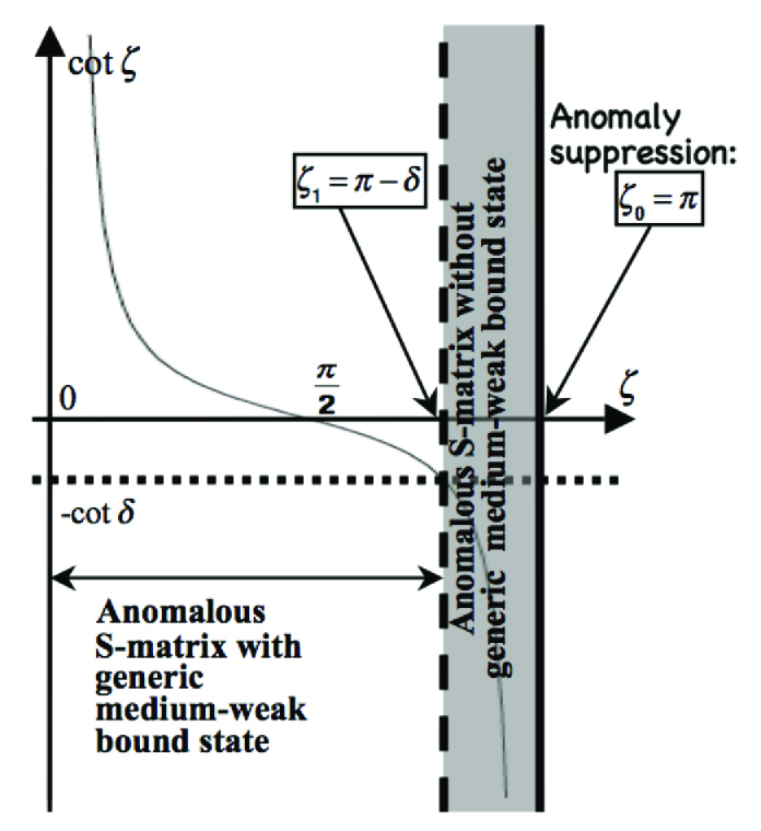
Figure 1: Self-adjoint extensions in the medium-weak coupling regime. The parameters $\delta\equiv\pi s/2$ (with $0<\delta<\pi/2$) and $\zeta\equiv\left(z+\delta\right)/2\pmod{2\pi}$ are defined. The region “without generic medium-weak bound state” corresponds to $\varrho^{({\rm SA})}(z)=F_{+}^{({\rm SA})}(z)/F_{-}^{({\rm SA})}(z)<0$ [see Eqs. (14) and (16)]; strictly speaking, for some rational values of $s$, this region may admit a bound state as well. The value $z=z_{0}$ effectively suppresses the medium-weak anomaly.

which can be obtained by comparison with the extensions (11) near the singularity. These states, as shown in Fig. 1, exist for $z\in{\mathcal{S}}\equiv[0,z_{1})\cup(z_{0},2\pi)$, independently of the value of $0<s<1$, where $z_{1}=2\pi\!-\!3\pi\,s/2$ and $z_{0}=2\pi\!-\!\pi\,s/2$ are the formal limits of $\kappa=0$ and $\kappa=\infty$ respectively. Curiously, their existence is maintained even in the cases when the potential is repulsive.

A more careful analysis of the S-matrix (21) reveals additional properties of the self-adjoint-extended Hamiltonians. The poles of Eq. (21) in the complex $k$ plane are located at the points

$$k_{n}=i\mu\left[{\varrho}^{({\rm SA})}(z)\right]^{1/2s}\,e^{n\pi i/s}\;,$$ (23)

where $n$ is an integer, and the sign of ${\varrho}^{({\rm SA})}(z)$ in $k_{0}=i\mu\left[{\varrho}^{({\rm SA})}(z)\right]^{1/2s}$ shows again the separation of the interval $z\in[0,2\pi)$ in two parts: $\mathcal{S}$, where it is positive, and its complement ${\mathcal{T}}\equiv(z_{1},z_{0})$, where it is negative. The first region, $\mathcal{S}$, is seen to reproduce the bound state energy (22) from $E_{0}=k_{0}^{2}$, with $n=0$ in Eq. (23). However, the multiplicity factor $e^{2in\delta}$ in Eq. (23), with $\delta=\pi s/2$, typically generates additional poles; these are located symmetrically at points of the same modulus with a phase increment $2\delta$. Whenever $2\delta$ is a rational number times $2\pi$, which occurs for rational values of $s$, these form a finite set; however, for irrational values of $s$, they consist of an infinite set of distinct poles. The second region, $\mathcal{T}$, involves a principal value $k_{0}=i\mu\left|{\varrho}^{({\rm SA})}(z)\right|^{1/2s}\,e^{i\delta}$, which typically lies in the complex plane and away from the positive imaginary axis; in addition, the multiplicity factor $e^{2in\delta}$ unfolds a similar pole structure as for $\mathcal{S}$, but rotated through a phase $\delta$. Most of these poles, for $z$ values both in $\mathcal{S}$ and in $\mathcal{T}$, do not have a simple interpretation; however, some of them may be interpreted as resonances, while occasionally, for specific rational values of $s$, some may generate a virtual state or even a single bound state in $\mathcal{T}$ [with the latter occurring for $s=(2p-1)/4q$, when $p$ and $q$ are positive integers, such that $s<1$]. It should be noticed that this polology of the self-adjoint extensions exists for all values of $z$ except for $z_{0}$ and $z_{1}$.

IV Effective-field-theory approach: Conformal S-matrix

In this section we will address the main theme of our paper: the resolution of the physical indeterminacy of self-adjoint extensions via physical regularization and renormalization. In simple terms, while the self-adjoint method deals with the symptoms of the “quantum illness” at the level of the boundary conditions, only the effective field approach tackles the underlying cause of the singular behavior.

Furthermore, the S-matrix framework of Sec. II serves as the analytical basis for a comprehensive study of singular potentials and will be central to our proof of the inequivalence of the two methods for the long-range conformal interaction. The basic procedure was carried out in the previous section using self-adjoint extensions. In this section, following a similar methodology, we will derive the more stringent conditions arising from a regularization and renormalization of the conformal potential.

IV.1 Regularized conformal S-matrix and coupling regimes

As anticipated in Sec. I, the presence of a singularity requires an effective treatment. In this renormalization context, singular quantum mechanics calls for the use of a cutoff $a$ and an ultraviolet regularizing core $V^{(<)}({\bf r})$ for $r\lesssim a$. As a result, the functions $u_{\pm}(r)$ can be used to provide the required matching through the dimensionless logarithmic derivative renormalization_CQM

$${\mathcal{L}}\equiv\left.r\,\frac{d\ln\left[u(r)/r^{\gamma/4}\right]}{dr}\right|_{r=a}\;.$$ (24)

In essence, Eq. (24) effects the regularization, as shown below for conformal quantum mechanics and other singular interactions. It should be noticed that the unconventional normalization of Eq. (24) is specifically tailored to the computations for the conformal and other singular interactions.

In this paper we show that there are no additional physical regimes, other than the weak and strong, under reasonable conditions supported by a large class of realizations. In effect, from the regularization procedure, the coefficient $\Omega$ can be computed as a function of $a$,

$$\Omega(a)=-\rho\,\left(\frac{ka}{2}\right)^{-2s}\;,$$ (25)

with

$$\rho=\frac{F_{+}}{F_{-}}\;$$ (26)

given in terms of

$$F_{\pm}=\Gamma(1\pm s)\;\left(\frac{{\mathcal{L}}}{s}\pm 1\right)\;.$$ (27)

From the generic Eq. (20), the singularity parameter (25) yields the regularized S-matrix

$$\tilde{S}\equiv\hat{S}\,e^{i\pi s}=\frac{e^{i\pi s}\,\left(ka/2\right)^{2s}-\rho}{e^{-i\pi s}\,\left(ka/2\right)^{2s}-\rho}\;.$$ (28)

Notice the formal similarity between Eqs. (21) and (28), Eqs. (15) and (25), and between Eqs. (16) and (26). However, with the physical regulator $a$, the functional form of Eq. (28) shows the existence of a critical condition at the index value $s=0$, in the transition from positive real $s$ to an imaginary value, according to Eq. (8). Consequently, when $a\rightarrow 0$, two and only two distinct regimes emerge:
(i) Weak or subcritical ($s$ real), with a “quasi-free S-matrix”

$$\left.\tilde{S}\right|_{\rm quasi\;free}=\hat{S}e^{i\pi s}=1\;,$$ (29)

for which the limit is well defined. By comparison with the original generic solution, it is observed that the more divergent power, $u_{-}(r)$, in Eq. (5) is rejected and no outstanding indeterminacy remains.
(ii) Strong or supercritical ($s=i\Theta$ pure imaginary), for which the regularized S-matrix (28) has an ill-defined limit. In contradistinction to the subcritical case, it is observed that the boundary-condition indeterminacy cannot be resolved by the ordinary techniques of regular quantum mechanics.

IV.2 Effective-field-theory resolution of the physical indeterminacy of self-adjoint extensions

The main conclusion of Sec. III is the indeterminacy of the self-adjoint extension method, with the appearance of an unusual bound state for medium-weak coupling. We will now show that this non-uniqueness can be physically resolved by adopting the effective approach outlined above.

The selection of a physically preferred self-adjoint extension can be established by comparing the coefficients in the expansions of the exterior solutions $u_{1,2}(r)$ for the self-adjoint extensions with the effective regularized solutions. This can be done step by step, verifying self-consistency, or more simply by direct comparison of the S-matrices for both approaches. The latter procedure involves identifying Eq. (21) with Eq. (28) in the medium-weak coupling regime, with the effective S-matrix collapsing to the quasi-free form (29). Consequently, in Eq. (21) the choice

$$\left.\tilde{S}\right|_{\rm quasi\;free}=1\Rightarrow{\varrho}^{({\rm SA})}(z)=\infty\Rightarrow z_{0}=2\pi\!-\!\pi\,s/2\;,$$ (30)

is enforced, and a unique correct extension is selected by the effective renormalization interpretation. The same conclusion is reached by direct comparison of Eqs. (15) and (25). In a simpler framework, this amounts to a straightforward regularization meetz:64 via the steps leading to Eq. (28). Moreover, Eq. (13) shows that this is equivalent to the rejection of the more singular solution. Thus, this procedure lifts the indeterminacy in the boundary condition; in short, the extension with $z=z_{0}$ is selected by the physical regularization procedure. At a purely formal level, in terms of the bound-state sector, Eq. (30) corresponds to the bound-state scale $\kappa\rightarrow\infty$; no such bound state exists, but this procedure gives the correct asymptotics, $\Omega=-e^{-i\pi s}$ for a formal bound state [with $S=\infty$ in Eq. (20)]—such that $a\rightarrow 0$ and $\kappa\rightarrow\infty$ simultaneously in $\Omega\propto\left(\kappa a/2\right)^{-2s}$.

Incidentally, the SO(2,1) symmetry seems to play a selective role in this problem as well. In effect, the self-adjoint-extended S-matrix (21) breaks the conformal symmetry for all self-adjoint extensions except $z=z_{0}$ and $z=z_{1}$, as can be seen by inspection of its explicit dependence with respect to the scale $k$. The corresponding symmetry-breaking solutions can only be regarded unphysical when this occurs in the presence of the symmetry-preserving extensions. Moreover, the extension $z=z_{1}$ can be further excluded as it does not reproduce the correct S-matrix for the free particle in three dimensions. This line of argumentation again shows that the correct physical self-adjoint extension is provided by $z=z_{0}$.

In conclusion, the choice $z=z_{0}$ circumvents the apparent quantum anomaly of the S-matrix (21), including the removal of a medium-weak bound state Friedrichs . The symmetry breaking can be traced to extraneous delta-function potentials zorbas:80 , which are ordinarily not warranted by the long-range conformal interaction. In this medium-weak anomaly suppression, when the phenomenology does not support extra interactions, the leading physics is governed by symmetry and regularization. By contrast, we will see that an anomaly cannot be circumvented for strong coupling.

IV.3 The Nontrivial Physics of the Conformal Strong Coupling

We will now examine the physics of the effective renormalization procedure for strong coupling. As it turns out, their deceptively similar spectra hide profound physical differences, which are related to the precise origin of the quantum anomaly.

Our comparative analysis is again displayed by the S-matrix. In the supercritical case, with $s=i\Theta$, the function $\rho$ of the renormalization approach in Eq. (26) turns into a pure phase because $F_{+}^{*}=-F_{-}$, as shown by Eq. (27). Thus, Eq. (28) gets replaced by

$$\tilde{S}\equiv\hat{S}\,e^{-\pi\Theta}=\frac{e^{-\pi\Theta}\,\left(k/\mu\right)^{2i\Theta}+e^{-2i\left(\Theta\,\gamma_{\Theta}+\chi\right)}\,\left(2/\mu a\right)^{2i\Theta}}{e^{\pi\Theta}\,\left(k/\mu\right)^{2i\Theta}+e^{-2i\left(\Theta\,\gamma_{\Theta}+\chi\right)}\,\left(2/\mu a\right)^{2i\Theta}}\;,$$ (31)

where $\mu$ is an arbitrary scale, $\gamma_{\Theta}=-\left\{{\rm phase}\left[\Gamma(1+i\Theta)\right]\right\}/\Theta$, and $\chi=\pi\,f_{0}={\rm phase}\left(1+i{\mathcal{L}}/\Theta\right)$. Then, Eq. (31) can be physically interpreted by applying the well-known limit-cycle behavior that arises from the renormalization of the conformal potential with a regularizing core beane:01 ; braaten:04 ; hammer:06 as $a\rightarrow 0$. This limit cycle is easily seen from the oscillatory nature of the imaginary powers in Eq. (31), with the core renormalization encoded in $\chi$ through the logarithmic derivative ${\mathcal{L}}$, Eq. (24). In this novel approach, it is easy to see the emergence of nontrivial bound states through the poles of the S-matrix, with a reference level $E_{0}=-\mu^{2}$ defined in terms of the renormalization scale $\mu$. Consequently, Eq. (31) turns into the renormalized S-matrix

$$\tilde{S}\equiv\hat{S}\,e^{-\pi\Theta}=\frac{e^{-\pi\Theta}\,\left(k/\sqrt{|E_{0}|}\right)^{2i\Theta}-1}{e^{\pi\Theta}\,\left(k/\sqrt{|E_{0}|}\right)^{2i\Theta}-1}\;,$$ (32)

where $E_{0}=-(2e^{-\gamma_{\Theta}}/a)^{2}e^{-2\pi f_{0}/\Theta}$. In particular, from its poles, the S-matrix yields the bound state spectrum by considering the multiplicity arising from the imaginary nature of the exponent $i\Theta$ in Eq. (32). The ensuing energy levels are

$$E_{n}=E_{0}\,\exp\left(-\frac{2\pi n}{\Theta}\right)\;,$$ (33)

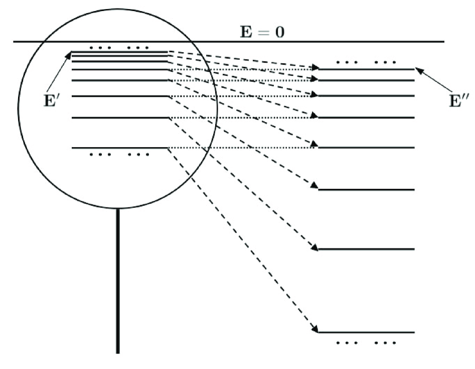
Figure 2: The strong-coupling conformal spectrum displays a residual discrete scale invariance, under magnifications $E^{\prime\prime}/E^{\prime}$. This is limited by infrared and ultraviolet cutoffs.

whose most important property is geometric scaling, which is uniquely determined by discrete scale symmetry: Given two bound-state energies $E^{\prime}$ and $E^{\prime\prime}$, the spectrum is invariant under the magnification $E^{\prime\prime}/E^{\prime}$ (see Fig. 2). Moreover, from Eq. (2), the corresponding bound states can be found by enforcing the condition $\hat{S}=\infty$, which leads to the familiar states $u(r)\propto\sqrt{|E_{n}|\,r}\;K_{i\Theta}(\sqrt{|E_{n}|}\,r)$, in terms of the Macdonald function macdonald_function , as shown in Refs. renormalization_CQM ; EFT_singular . In essence, a properly physical quantum anomaly is realized for strong coupling, where binding occurs [as in Eq. (33)] and the S-matrix (32) is manifestly scale dependent. Nevertheless, an important restriction is in order: Eqs. (32) and (33) are limited in energy by the effective renormalization procedure, thus guaranteeing the physical boundedness from below of the effective Hamiltonian.

The above prediction of the effective renormalization method can be compared with its counterpart for the self-adjoint extensions. The latter can be obtained in the strong-coupling regime through a generalization of Eq. (21) for $s=i\Theta$; by inspection of the near-singularity behavior in Eq. (12), it follows that Eq. (14) still applies, with the modified functions $\phi_{\pm}(s=i\Theta)=\pm i\pi\Theta/4$. As expected, the S-matrix (21) retains a $z$-parameter ambiguity but is otherwise similar to Eq. (32) in its analytic structure. Not surprisingly, the determination of its poles again involves the complex root required by inversion of the exponent $i\Theta$. The ensuing symmetry-breaking strong-coupling energies are structured with an infinite multiplicity factor $e^{-2\pi n/\Theta}$, which is the analogue of the phase factor in Eq. (23), but for an imaginary index. Therefore, the energy spectrum of the self-adjoint extensions is formally identical to that of Eq. (33), where the real nature of the energies is guaranteed by the fact that ${\varrho}^{({\rm SA})}(z)$ is a pure phase in this coupling regime. Thus, at first sight in Fig. 2, both methods appear to give the geometric conformal tower. However, a critical difference should be highlighted: while an effective renormalization approach has a lower bound or base energy value by construction (as dictated by the ultraviolet physics), the self-adjoint extensions generate a “conformal tower” devoid of lower bound. Thus, with reference to Fig. 2, the complete tower extending to minus infinite energy corresponds to the self-adjoint extensions, while the renormalized spectrum further breaks the symmetry by terminating the sequence from below. In short, from the conformal SO(2,1) symmetry viewpoint: (i) the full-fledged residual discrete symmetry is realized in the self-adjoint extensions; (ii) in the physical spectrum with energies (33), the residual discrete symmetry is terminated from below, within an effective-field theory interpretation.

In short, while a spectrum not bounded from below is mathematically harmless, such solution is physically untenable as it signals an unavoidable instability of the quantum system. This property ultimately persists because the self-adjoint extensions maintain the unadulterated form of the singularity—this is seen to be one aspect of the behavior known as “the fall to the center” landau:77 . By contrast, the effective renormalization discussed above restores the physically mandatory boundedness, in another example of a phenomenon called “quantum mechanical resuscitation” stevenson:84 .

V Conclusions and outlook

In this paper we have shown that the often-assumed equivalence between self-adjoint extensions and renormalization for singular potentials fails to be valid for long-range interactions. Our conclusions broadly show that a physically-based analysis of singular potentials resolves the physical indeterminacy of self-adjoint extensions within the modern effective renormalization paradigm.

For the long-range conformal interaction, we have found major differences between the two methods. First, in the medium-weak coupling regime, the self-adjoint extensions typically include a bound state. By contrast, a physical regularization performs a medium-weak anomaly suppression compatible with the conformal symmetry, fully resolving the physical indeterminacy of self-adjoint extensions. Second, in the strong-coupling regime, despite the formal similarity of the respective conformal towers of bound states, the self-adjoint-extended Hamiltonians fail to be bounded from below, unlike their renormalized counterparts.

The physical consequences of our analysis are noteworthy even from the phenomenological viewpoint. First, a hypothetical realization of the medium-weak bound state would effectively imply the loss of the critical nature of $\lambda^{(*)}$. Thus, the observed sharp criticality, revealed by the absence of the medium-weak state, is a confirmation of the predicted anomaly suppression: (i) dipole-bound anions molecular_dipole_anomaly have an experimentally verified critical dipole moment $p^{(*)}\neq 0$; (ii) in QED₃ with $N_{f}$ Dirac-fermion flavors gusynin1 , the critical fermion number $N^{(*)}=128/(3\pi^{2})$ is given by conformal quantum mechanics and also expected from alternative theoretical frameworks—moreover, this is a feature of dynamical chiral symmetry breaking in gauge theories, including applications in extra dimensions gusynin2 . Second, in the strong-coupling sector, the bounded tower of conformal states (33) with a sharp critical coupling $\lambda^{(*)}$ is the essence of the Efimov effect for three-body contact interactions efimov_effect ; Macek:06 and of the realizations discussed above. Third, the medium-weak bound state has been invoked in black hole thermodynamics near_horizon through the static limit leading to a critical coupling for the near-horizon physics; however, given the physical indeterminacy of the self-adjoint extension method, one should not ascribe any fundamental meaning to these calculations—as it turns out, the effective near-horizon quantum-mechanical equations BH_thermo_CQM ; semiclassical_BH involve the strong-coupling sector. Finally, the medium-weak regime may be relevant for the question of cosmic censorship and the geometric singularity of black holes, due to the universal conformal behavior $\sim 1/x^{2}$ of the near-singularity field equations with respect to the tortoise coordinate Papdopoulos ; however, our paper suggests that caution must be exercised in the use of self-adjoint extensions for the near-singularity physics.

Incidentally, many of the ideas of the previous sections—using a physical regularization with an ultraviolet core—admit a straightforward generalization to long-range strictly singular interactions $V({\bf r})=-\lambda\,r^{-\gamma}$, with $\gamma>2$ and $\lambda>0$ in Eq. (1). However, this generalized model is not scale invariant and the dimensions of $\lambda$ play a central role; with the standard arguments, considering this as a $(0+1)$-dimensional effective field theory EFT , one expects that some of the advantages of the renormalizable conformal interaction may be lost when $\gamma>2$. Thus, the competition between the kinetic and potential terms manifests in a different manner: as the physics is ultimately modified in the presence of an ultraviolet scale $L_{UV}$ or cutoff $a$, a comparison of the competing terms yields the condition $\lambda^{1/(\gamma-2)}\gg L_{UV}\sim a$. In addition, the semiclassical approximation is asymptotically exact with respect to the near-singularity behavior semiclassical_BH ; consequently, the solutions follow from the usual WKB outgoing/ingoing near-singularity waves $u_{\pm}(r)$, combined with a matching procedure with a regularizing core for the removal of divergences—this is known to involve a limit-cycle behavior beane:01 . Then, $\Omega\propto\exp\!\left[-4\,i\,\lambda^{1/\gamma}\,\left(k^{1-2/\gamma}-\mu^{1-2/\gamma}\right)/\left(\gamma-2\right)\right]$, with $E_{0}=-\mu^{2}$ being an energy scale; in turn, the S-matrix (7) reproduces the relevant physics, with its poles corresponding to the leading-order renormalized energies $E_{n}/E_{0}=\left[1-\left(\gamma-2\right)\,\pi n/\left(2\,\lambda^{1/\gamma}\left|E_{0}\right|^{(\gamma-2)/2\gamma}\right)\right]^{2\gamma/\left(\gamma-2\right)}$ and reduces to the conformal counterparts in the limit $\gamma\rightarrow 2$, with $\sqrt{\lambda}\rightarrow\Theta$ (the Langer replacement semiclassical_BH ). Therefore, for the strictly singular long-range interactions, one concludes that: (i) the critical coupling is zero; (ii) there is no analog of the medium-weak coupling; (iii) the strong-coupling regime is similar to the conformal one, but without scale symmetry, with an ultraviolet cutoff suppressing the unphysical behavior of a spectrum originally not bounded from below. Relevant examples in molecular systems vogt_wannier ($\gamma=4$) and for the nucleon-nucleon interaction beane:01 ($\gamma=3$) are well known. The case with $\gamma=4$ can also be found in extremal black holes and D-brane dynamics park_D-brane_IQP and will be discussed elsewhere.

- (1) W. M. Frank, D. J. Land, and R. M. Spector, Rev. Mod. Phys. 43 (1971) 36; and references therein.
- (2) L. D. Landau and E. M. Lifshitz, Quantum Mechanics, third ed., Pergamon Press, Oxford, 1977, pp. 114–117.
- (3) J. von Neumann, Math. Ann. 102 (1929) 49131.
- (4) N. I. Akhiezer and I. M. Glazman, Theory of Linear Operators in Hilbert Space, Frederick Ungar Publishing Co., New York, 1961, Volume 2; M. A. Naimark, Linear Differential Operators, Frederik Ungar Publishing Co., New York, 1968, Part II, Chapter IV.
- (5) M. Reed and B. Simon, Methods of Modern Mathematical Physics, Academic Press, New York, 1972, Volume 2, p. 135.
- (6) S. Albeverio, F. Gesztesy, R. Høegh-Kron, and H. Holden, Solvable Models in Quantum Mechanics, Springer-Verlag, New York, 1988.
- (7) R. Jackiw, in: M. A. B. Bég Memorial Volume, A. Ali and P. Hoodbhoy (Eds.), World Scientific, Singapore, 1991.
- (8) K. Huang, Quarks, Leptons, and Gauge Fields, second ed., World Scientific, Singapore, 1992, Sections 10.7 and 10.8.
- (9) C. Manuel and R. Tarrach, Phys. Lett. B 268 (1991) 222; C. Manuel and R. Tarrach, 301 (1993) 72; K. S. Gupta and S. G. Rajeev, Phys. Rev. D 48 (1993) 5940.
- (10) H. E. Camblong, L. N. Epele, H. Fanchiotti, and C. A. García Canal, Phys. Rev. Lett. 85 (2000) 1590; H. E. Camblong, L. N. Epele, H. Fanchiotti, and C. A. García Canal, Ann. Phys. (N.Y.) 287 (2001) 14; H. E. Camblong, L. N. Epele, H. Fanchiotti, and C. A. García Canal, Ann. Phys. (N.Y.) 287 (2001) 57.
- (11) H. E. Camblong and C. R. Ordóñez, Phys. Rev. D 68 (2003) 125013; H. E. Camblong and C. R. Ordóñez, Phys. Lett. A 345 (2005) 22.
- (12) H. E. Camblong, L. N. Epele, H. Fanchiotti, C. A. García Canal, and C. R. Ordóñez, Phy. Rev. A 72 (2005) 032107.
- (13) K. G. Wilson, Rev. Mod. Phys. 47 (1975) 773; J. Polchinski, Nucl. Phys. B 231 (1984) 269; J. Polchinski, hep-th/9210046.
- (14) H. E. Camblong and C. R. Ordóñez, Phys. Rev. D 71 (2005) 124040.
- (15) G. Esposito, J. Phys. A: Math. Gen. 31 (1998) 9493.
- (16) H. Narnhofer, Acta Phys. Austr. 40 (1974) 306.
- (17) D. Birmingham, K. S. Gupta, and S. Sen, Phys. Lett. B 505 (2001) 191; K. S. Gupta and S. Sen, Phys. Lett. B 526 (2002) 121.
- (18) H. E. Camblong and C. R. Ordóñez, Phys. Rev. D 71 (2005) 104029.
- (19) K. Srinivasan and T. Padmanabhan, Phys. Rev. D 60 (1999) 024007; T. Padmanabhan, Phys. Rept. 406 (2005) 49; and references therein.
- (20) V. P. Gusynin, A. H. Hams, and M. Reenders, Phys. Rev. D 53 (1996) 2227.
- (21) R. Jackiw, Phys. Today 25 (1) (1972) 23.
- (22) V. de Alfaro, S. Fubini, and G. Furlan, Nuovo Cimento A 34 (1976) 569.
- (23) This is the analogue of the floating-point renormalization scale: S. Weinberg, The Quantum Theory of Fields, Cambridge University Press, Cambridge, UK, 1995.
- (24) K. Meetz, Nuovo Cimento 34 (1964) 690.
- (25) This is the Friedrichs extension; see B. Simon, Quantum Mechanics for Hamiltonians Defined as Quadratic Forms, Princeton University Press, Princeton, 1971.
- (26) J. Zorbas, J. Math. Phys. 21 (1980) 840.
- (27) S. R. Beane, P. F. Bedaque, L. Childress, A. Kryjevski, J. McGuire, and U. van Kolck, Phys. Rev. A 64 (2001) 042103; and references therein.
- (28) E. Braaten and D. Phillips, Phys. Rev. A 70 (2004) 052111.
- (29) H.-W. Hammer and B. G. Swingle, Ann. Phys. (N.Y.) 321 (2006) 306.
- (30) A. Erdélyi and the Staff of the Bateman Manuscript Project (Eds.), Higher Transcendental Functions, McGraw-Hill, New York, 1953, Volume II, Chapter VII.
- (31) P. M. Stevenson, Phys. Rev. D 30 (1984) 1712.
- (32) H. E. Camblong, L. N. Epele, H. Fanchiotti, and C. A. García Canal, Phys. Rev. Lett. 87 (2001) 220402.
- (33) V. Gusynin, M. Hashimoto, M. Tanabashi, and K. Yamawaki, Phys. Rev. D 65 (2002) 116008.
- (34) V. Efimov, Phys. Lett. B 33 (1970) 563; V. Efimov, Sov. J. Nucl. Phys. 12 (1971) 589; V. Efimov, Comments Nucl. Part. Phys. 19 (1990) 271.
- (35) The Efimov effect, with the full-fledged physics of conformal quantum mechanics, has been recently extended to the three-body contact interaction of spin 1/2 fermions with nonzero angular momentum: J. H. Macek and J. Sternberg, Phys. Rev. Lett. 97 (2006) 023201.
- (36) G. Papadopoulos, Class. Quant. Grav. 21 (2004) 5097; M. Blau, D. Frank, and S. Weiss, hep-th/0602207.
- (37) E. Vogt and G. H. Wannier, Phys. Rev. 95 (1954) 1190.
- (38) D. K. Park, S. N. Tamaryan, H. J. W. Müller-Kirsten, and J.-z. Zhang, Nucl. Phys. B 594 (2001) 243.