LG (Landau-Ginzburg) in GL (Gregory-Laflamme)

Abstract:

This paper continues the study of the Gregory-Laflamme instability of black strings, or more precisely of the order of the transition, being either first or second order, and the critical dimension which separates the two cases. First, we describe a novel method based on the Landau-Ginzburg perspective for the thermodynamics that somewhat improves the existing techniques. Second, we generalize the computation from a circle compactification to an arbitrary torus compactifications. We explain that the critical dimension cannot be lowered in this way, and moreover in all cases studied the transition order depends only on the number of extended dimensions. We discuss the richer phase structure that appears in the torus case.

1 Introduction and summary

In the presence of a compact dimension Gregory and Laflamme (GL) discovered that uniform black strings are perturbatively unstable below a certain critical dimensionless mass density [1]. The order of the transition can be computed by following perturbatively the branch of non-uniform solutions which emanates from the critical GL string, as first shown by Gubser in the case of a five-dimensional spacetime [2] where the transition is first order. That calculation was generalized by one of us (ES) to arbitrary spacetime dimensions with the surprising result that the transition is first order only for $D<D^{*}=``13.5"$ while it is second order for higher dimensions [3]. Here first order means a transition between two distinct configurations, while a second order transition is smooth – the uniform string changes smoothly into a slightly non-uniform string. Kudoh and Miyamoto [4] repeated the calculation in the economical Harmark-Obers coordinates [5], confirmed previous results and observed that in the canonical ensemble the critical dimension actually changes from $D^{*}=``13.5"$ to $D^{*}_{can}=``12.5"$. All this data constitutes an important piece in the construction of the phase diagram for this system (see [6] and [7] for a review).

The present paper includes two main results. First, we show how to somewhat improve the existing method of calculating the transition order by employing a Landau-Ginzburg perspective (the basic idea was described already in Appendix A of [8]). Secondly, we generalize from the usual $\mathbb{S}^{1}\equiv{\bf T}^{1}$ compactification to an arbitrary torus compactification ${\bf T}^{p}$.

Landau-Ginzburg improvement to the method. In Section 2 we review our set-up and how the description of phase transitions is achieved by the Landau-Ginzburg (LG) theory, where one expands the free energy of the system around the critical point in powers of order parameters. In particular, it is known that as long as the coefficient of a certain cubic term in the free energy is non-vanishing then the transition is first order. If the cubic term vanishes, for instance due to a parity symmetry such as in our case, then it is the sign of the coefficient of a certain quartic term, which we denote by ${\cal C}$, that determines whether the transition is first order or higher (of course if this term vanishes one has to go to higher terms). A simpler and more intuitive form of this criterion, which is, alas, less general and does not apply in our case (as expanded in the text), is that the transition is second order iff the critical solution is a (local) minimum of the free energy.

Before we can compare the Landau-Ginzburg method with Gubser’s method, we should recall the features of the latter. There one computes order by order the metric of the static non-uniform string branch emanating from the critical GL string. The first order is nothing but the GL mode. At the second order one computes the back-reaction. Finally the third order is computed, or more precisely only the first harmonic along the compact dimension, from which one can finally compute the leading coefficients of the changes in mass and entropy, $\eta_{1},~{}\sigma_{2}$ of the new branch. The sign of these two quantities is correlated and determines the order of the transition.

At first sight the two methods look quite different. However, we show that in the LG method one also needs to precisely compute the second order back-reaction to the metric. The third order however is not required in LG (thereby avoiding the solution of a set of linear differential equations with sources). Rather one needs only to expand the action to an appropriate quartic order, to substitute in the results from the first and second orders and perform certain integrals that add up to the constant whose sign determines the order.

A way to understand the simplification is the following: in Gubser’s method one computes the third order, but it turns out that all that is really needed is the projection of the third order onto the GL mode. That is precisely the reason why the first harmonic sufficed (as the GL mode is in the first harmonic). Our substitution into the quartic order of the free-energy achieves exactly that, without the need to compute other properties of the third order.

In Section 3 we perform the “Landau-Ginzburg” calculation for an $\mathbb{S}^{1}$ compactification in various dimensions and verify that we get the same bottom-line coefficients $\eta_{1},~{}\sigma_{2}$ as in the previous method, see table 3.

Torus compactification. It is interesting to generalize the compactifying manifold, and the simplest option beyond the circle $\mathbb{S}^{1}\equiv{\bf T}^{1}$, is a product of circles, or more generally a $p$-torus ${\bf T}^{p}$. The number of extended spacetime dimensions is denoted by $d$ and the total spacetime dimension is $D=d+p$. The critical GL density for such a torus compactification is easily found to be given in terms of the shortest vector in the reciprocal lattice [9].

We proceed to analyze the transition order in Section 4. First, we motivate restricting ourselves to square torii. Basically, we view the space of torii as having two boundaries – on the one hand highly asymmetrical torii, where one (or more) dimensions are much larger than the rest, and on the other hand highly symmetrical torii such as the square torus. Since the limit of a highly asymmetrical torus reduces to the case of a lower dimensional torus (mostly the well-understood case of $\mathbb{S}^{1}$ compactification), we argue that by studying the opposite limit of a highly symmetrical torus, we achieve an understanding of both limits and thereby also some understanding of the intermediate region of general torii.

For a square ${\bf T}^{p}$ torus compactification, $p$ modes turn marginally tachyonic at the same (GL) point. We find that the constant ${\cal C}$ is replaced by a $p\times p$ quadratic form ${\cal C}^{ij}$, in order to allow for the various possible directions in the (marginally) “tachyon space”, and that the transition is second order iff ${\cal C}^{ij}$ is positive for all directions. Namely, it is enough that there is a single direction in tachyon space which sees a first order transition for the transition to be one. Taking into account the ${\bf T}^{1}$ results we may immediately deduce that the critical dimension cannot be lower than in the ${\bf T}^{1}$ case with the same number of extended dimensions, $d$. This shows that the indicators of [9] for second order transition at lower dimensions, which were part of the motivation for this work, were misleading, as further discussed in the text.

Due to the high degree of symmetry of the square torii ${\cal C}^{ij}$ consists only of two independent entries: all the diagonal entries are the same, denoted by ${\cal C}^{=}$, and all the off-diagonal entries are the same, denoted by ${\cal C}^{\neq}$. Since the diagonal term is precisely the one computed in the ${\bf T}^{1}$ compactification, we set to compute the off-diagonal term. Due to the symmetry ${\cal C}^{\neq}$ is the same for all $p$ and for that purpose it suffices to consider $p=2$, namely we consider the square ${\bf T}^{2}$ torus. The only parameter remaining is the number of extended dimensions.

In practice we do not compute ${\cal C}^{\neq}$ directly, but rather the effective ${\cal C}$ for a diagonal direction in tachyon space, which we denote by $\bar{\cal C}$. Then we solve for ${\cal C}^{\neq}$ which is a linear combination of ${\cal C}^{=},\,\bar{\cal C}|_{p=2}$.

In Section 5 we proceed to the actual calculation for ${\bf T}^{2}$. Once we have chosen the diagonal direction in tachyon space we are not bothered any longer by the presence of several (marginally) tachyonic modes. However, the number of metric components involved in the calculation (back reaction and quartic coefficient) is larger than in the ${\bf T}^{1}$ case. Certain discrete symmetries are found to be helpful in simplifying the calculation. The calculations and results are described in detail, thereby applying our improved method to achieve new results.

In Section 6 we analyze the results and their implications. We find that for all the studied values of $d$ where the ${\bf T}^{1}$ transition is second order, the ${\bf T}^{p}$ transition is also second order for all $p$. Combining this result with observation mentioned above we conclude that the transition order for square torii shows some robustness in that it depends only on $d$, the number of extended dimensions, and not on $p$.

In addition we discuss some subtler implications, including the finding that for almost all $d$ the diagonal direction in tachyon space is disfavored relative to turning on a tachyon in a single compact dimension, and in this sense we have spontaneous symmetry breaking.

The appendices A, B contain the details of the full equations, of the numerical technique and summarize various numerical parameters.

2 Set-up and Landau-Ginzburg theory of phase transitions

2.1 Set-up

The Gregory-Laflamme instability and associated phase transition physics appear in the presence of compact dimensions, namely for backgrounds of the form $\mathbb{R}^{d-1,1}\times Y^{p}$ where $Y^{p}$ is any $p$-dimensional compact Ricci-flat manifold, $d\geq 4$ is the number of extended spacetime dimensions, and the total spacetime dimension is $D=d+p$.

The simplest compactifying manifold is a single compact dimension $Y=\mathbb{S}^{1}$. We shall first demonstrate the Landau-Ginzburg method in that context and then turn to $Y={\bf T}^{p}$, a square $p$-dimensional torus. We denote the torus size by $L$ and work with Euclidean time of period $\beta$ (corresponding to a canonical ensemble). Such backgrounds are characterized by a single dimensionless constant

$$\mu_{\beta}\propto{\beta\over L}~{},$$ (1)

where henceforth we shall omit the subscript $\beta$.

The non-rotating black objects in which we are interested are static and spherically symmetric (in the extended dimensions). After suppressing the time and the angular coordinates the remaining essential coordinates are $r$, the radial coordinate in the extended spatial directions, and $z^{i},~{}1\leq i\leq p$ the periodic coordinates $z^{i}\sim z^{i}+L$ which parameterize ${\bf T}^{p}$. Thus, the essential geometry has $p+1$ dimensions and we employ “cylindrical coordinates” $(r,z^{i})$.

The uniform black $p$-brane, the background around which we perturb (see figure 1) is given by

$$ds^{2}=ds^{2}_{\mbox{Schw}}+ds^{2}_{Y}$$ (2)

where $ds^{2}_{Y}$ is the metric on $Y^{p}$, which for our square torus is

$$ds^{2}_{Y}=\sum_{i=1}^{p}dz^{i}\,dz^{i}~{},$$ (3)

and $ds^{2}_{\mbox{Schw}}$ is the $d$-dimensional Schwarzschild black hole,

$$ds^{2}_{\mbox{Schw}}=-f(r)\,dt^{2}+\frac{1}{f(r)}\,dr^{2}+r^{2}\,d\Omega_{d-2}^{2},$$ (4)

where

$$f(r)=1-\left(\frac{r_{0}}{r}\right)^{d-3}~{},$$ (5)

and $d\Omega_{d-2}^{2}$ is the metric on the unit sphere. $r_{0}$ is related to the black hole mass, $M$, via [10]

$$r_{0}^{d-3}=\frac{16\,\pi\,G_{d}\,M}{(d-2)\,\Omega_{d-2}}~{},$$ (6)

where $G_{d}$ is the $d$-dimensional Newton constant, and $\Omega_{d-1}=d{\pi^{d/2}\over(d/2)!}=\frac{2\,\pi^{\frac{d}{2}}}{\Gamma(\frac{d}{2})}$ is the area of a unit sphere $S^{d-1}$. In Euclidean signature the space-time ends at the horizon. As usual, requiring the absence of a conical singularity there fixes $\beta$, the asymptotic size of the Euclidean time direction, and it is given by

$$\beta={2\,\pi\over\kappa}={4\,\pi\over f^{\prime}(r_{0})}={4\,\pi\,r_{0}\over d-3}~{}.$$ (7)

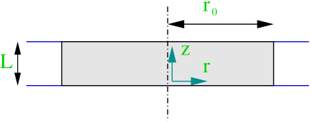
Figure 1: The uniform black string together with the definition of the cylindrical coordinates $(r,z)$. $r_{0}$ is the Schwarzschild radius.

Gregory and Laflamme discovered that the uniform black string solution (4) develops a $z$-dependent metric-instability below a certain critical (dimensionless) mass [1]. Equivalently, for a fixed $r_{0}$ there is a critical wavenumber

$$k\equiv 2\pi/L$$ (8)

for instability. At $k=k_{GL}$ the GL mode is marginally tachyonic, namely a zero-mode. In [1, 3] the critical GL lengths were obtained for Schwarzschild black holes in various dimensions (see table 1). From these the high $d$ asymptotic form was extracted and later proven analytically in [9] to be

$$k_{GL}\simeq\sqrt{d}\,{1\over r_{0}}~{}.$$ (9)

This means that for large $d$ the black string becomes unstable when $r_{0}/L\simeq\sqrt{d}$, namely when it is quite “fat” and this indicates that such a string would not decay into a black hole which would not “fit” inside the extra dimension.

d	4	5	6	7	8	9	10	11
$k_{GL}$	.876	1.27	1.58	1.85	2.09	2.30	2.50	2.69
d	12	13	14	15	19	29	49	99
$k_{GL}$	2.87	3.03	3.19	3.34	3.89	5.06	6.72	9.75

Table 1: The marginally static mode wavenumbers $k_{GL}$ in units of $r_{0}^{-1}$ as a function of $d$ [3, 9].

Having an unstable mode brings us to the issue of the order of the transition and the existence of additional phases. Rather than review the state of the art in this respect, we proceed in the next subsection to describe a somewhat novel method, which in section 3 will be shown to reproduce the known results and then will be used in section 5 to obtain new results.

2.2 Landau-Ginzburg: review and application

The central insight of the Landau-Ginzburg (LG) theory of phase transitions (see for example [11]) is that the nature of a phase transition can be deduced from the local behavior of the free energy around the critical solution. This local analysis is achieved by focusing on the low energy modes and zooming, namely carrying a Taylor expansion up to a specified order. For pedagogical reasons we divide the discussion into three steps: first we discuss a one-dimensional configuration space which is the simplest example, then the general configuration space and finally we utilize the translation symmetry in $z$ of our background to arrive at the final form of our formulae.

One-dimensional configuration space. The main idea can be demonstrated by a system with a configuration space consisting of a single variable $\tilde{\lambda}$ and by a control parameter $\mu$. The thermodynamics is encoded by the free energy function $F=F(\tilde{\lambda};\,\mu)$. Generically the free energy does not have a definite parity in $\tilde{\lambda}$, however sometimes additional symmetries of the system make the free energy even in $\tilde{\lambda}$, namely $F(-\tilde{\lambda};\,\mu)=F(\tilde{\lambda};\,\mu)$, which will be seen to hold in our case. This reflection symmetry implies that $\tilde{\lambda}=0$ is an extremum of the free energy (namely that the linear term in the Taylor expansion of $F$ in $\tilde{\lambda}$ around $\tilde{\lambda}=0$ vanishes). Assuming the existence of a critical solution with a marginally stable mode means that for some critical value of $\mu$ denoted by $\mu_{c}$ the quadratic term vanishes. Thus $F(\tilde{\lambda};\,\mu)=F_{0}(\mu)+{\cal A}\,(\mu-\mu_{c})\,\tilde{\lambda}^{2}+\dots$ where ${\cal A}$ is some constant, which we take to be positive without loss of generality (if ${\cal A}$ were negative we could redefine $\mu\to-\mu$). In order to determine the order of the transition it is sufficient to expand $F$ further as follows

$$F(\tilde{\lambda};\,\mu)=F_{0}(\mu)+{\cal A}\,\delta\mu\,\tilde{\lambda}^{2}+{\cal C}\,\tilde{\lambda}^{4}+\dots$$ (10)

where we defined

$$\delta\mu\equiv\mu-\mu_{c}$$ (11)

and ${\cal C}$ is another constant. Actually the whole function $F_{0}(\mu)$, is not required for the LG theory, only its expansion around $\mu\simeq\mu_{c}$, but we shall not be concerned with this expansion.

Once the constants ${\cal A},\,{\cal C}$ are determined the local thermodynamics may be deduced by following the form of the free energy and its extrema as $\mu$ is adjusted in the vicinity of $\mu_{c}$. Seeking additional extrema of (10) through ${\partial}F/{\partial}\tilde{\lambda}=0$ results in a new branch of extrema in addition to $\tilde{\lambda}=0$ namely,

$$\tilde{\lambda}^{2}_{b}=-{{\cal A}\,(\mu-\mu_{c})\over 2\,{\cal C}}~{},$$ (12)

where $\tilde{\lambda}_{b}=\tilde{\lambda}_{b}(\mu)$ describes the new branch. Note that since $\tilde{\lambda}^{2}\geq 0$ the new branch exists only for $\rm{sgn}(\mu-\mu_{c})=-sgn({\cal C})$ (locally). Depending on the sign of ${\cal C}$ we now get two possibilities which are depicted in figures 2, 3. For negative ${\cal C}$ the new branch exists only for $\mu>\mu_{c}$ and thus cannot serve as the end-state of the decay for $\mu<\mu_{c}$ (moreover it is unstable), and therefore a first order transition will occur into a phase at finite distance in configuration space. For positive ${\cal C}$ the new branch can and does serve as the end-point of the decay. The transition is smooth as one lowers $\mu$ below $\mu_{c}$. The difference in free-energies between the two phases is given by

$$F_{b}(\mu)-F_{0}(\mu)=F(\tilde{\lambda}_{b}(\mu);\mu)-F_{0}(\mu)=-{{\cal A}^{2}\,\,(\mu-\mu_{c})^{2}\over 4\,{\cal C}}=-{\cal C}\,\tilde{\lambda}_{b}^{4}~{}.$$ (13)

In particular there is a jump in the second derivative of $F_{b}-F_{0}$ with respect to $\mu$ at $\mu=\mu_{c}$. Hence by definition this transition is second order.

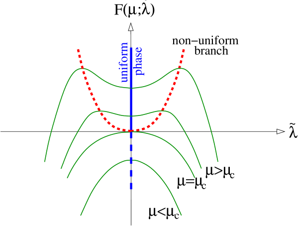
Figure 2: An illustration of a first order phase transition. A condensed plot showing two kinds of graphs. The thin solid lines show the free energy as a function of $\tilde{\lambda}$ for a sequence of $\mu$ values, while for the thick lines the vertical axis becomes $\mu$ (the horizontal remains $\tilde{\lambda}$) and they designate the various phases corresponding to the extremum of the free energy. The free energy has a minimum for $\mu>\mu_{c}$ that corresponds to the stable symmetric phase (thick solid line) which becomes unstable below $\mu_{c}$ (thick dashed line). It follows that the asymmetric phase branch emergent from the critical point (thick dotted line) is unstable since the free energy has a negative direction for $\mu\geq\mu_{c}$ at $\tilde{\lambda}=\tilde{\lambda}_{b}$. Note that the free energy in this phase is higher relative to that of the critical state.

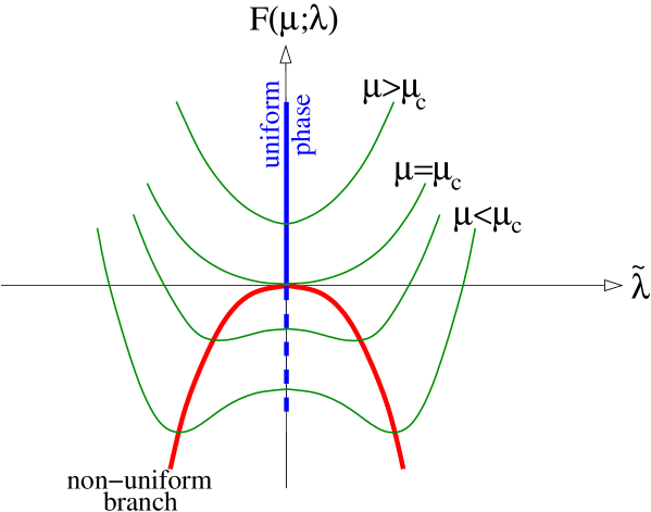
Figure 3: An illustration of a second order transition from a symmetric to an asymmetric phase, with the same condensed conventions as in figure 2. The free energy (designated by the thin solid line) has a minimum for $\mu>\mu_{c}$ corresponding to the stable symmetric phase (thick solid line) which becomes unstable below $\mu_{c}$ (thick dashed line). The free energy is at minimum also for $\mu=\mu_{c}$ and the minimum continuously moves away from $\tilde{\lambda}=0$, indicating that the emergent asymmetric phase is stable and has the asymmetry developing smoothly.

Given ${\cal A},\,{\cal C}$ and hence the form of $F=F(\mu)$ , which is the fundamental thermodynamic potential (in the canonical ensemble) we may find the rest of the thermodynamic quantities through the usual thermodynamic relations, as we now describe.

We particularize to the black branes in which case the temperature is $T\equiv\hbar/\beta$, and so the dimensionless temperature is $\theta=\mu^{-1}$ (1). Rephrasing (12) we obtain the leading behavior for the dimensionless temperature of the emergent branch

$${\delta\theta\over\theta}=-{\delta\mu\over\mu}={2\,{\cal C}\over{\cal A}\,\mu_{GL}}\tilde{\lambda}_{b}^{2}\equiv\theta_{1}\tilde{\lambda}_{b}^{2}.$$ (14)

The entropy and the mass of the solutions are $S=\mu^{2}{\partial}_{\mu}F$ and $M={\partial}_{\mu}(\mu\,F)$. We can find the coefficients of the second order variations of these quantities relative to the critical phase

$$s_{1}\equiv\left({\cal O}(\lambda^{2})~{}~{}{\rm of}~{}~{}\mu^{2}{\partial}_{\mu}{F(\mu)-F_{0}(\mu)\over F(\mu)}\right)={\mu_{GL}\,{\cal A}\over d-3},$$ (15)

$$m_{1}\equiv\left({\cal O}(\lambda^{2})~{}~{}{\rm of}~{}~{}-{\partial}_{\mu}{\mu\left[F(\mu)-F_{0}(\mu)\right]\over F(\mu)}\right)={\mu_{GL}\,{\cal A}\over d-2}.$$ (16)

The variation of the dimensionless mass,

$$\eta\equiv G_{d}M/L^{d-3}=G_{d}M\mu^{d-3}/\beta^{d-3}$$ (17)

in a canonical ensemble for given $\beta$ is comprised of two terms arising from variation of $M$ and $\mu$

$$\eta_{1} \equiv \left({\cal O}(\lambda^{2})~{}~{}{\rm of}~{}~{}{\delta\eta\over\eta}\right)=-(d-3)\theta_{1}+m_{1}=$$ (18)

$$= -2\,(d-3)\,{{\cal C}\over\mu_{GL}\,{\cal A}}+{1\over d-2}\,\mu_{GL}{\cal A}~{}.$$

Finally, we can also determine the entropy difference between non-uniform and the uniform phases with the same mass [2, 3]

$${S_{\rm non-uniform}\over S_{\rm uniform}} = 1+\sigma_{1}\lambda_{b}^{2}+\sigma_{2}\lambda_{b}^{4}+\dots,$$

$$\sigma_{1}=m_{1}-{d-3\over d-2}{s_{1}} \sigma_{2}=-{d-2\over 2\,(d-3)^{2}}\,m_{1}\,\eta_{1}.$$ , (19)

Note that vanishing of $\sigma_{1}$ is guaranteed by the first law.

Higher dimensional configuration space. While the discussion above reveals the essential point, it considers the free energy to be a function of a single configuration variable, while in our case it should be considered a function over the space of all metrics with fixed boundary conditions, which is an infinite dimensional space. More explicitly

$$-\beta\,F[g_{\mu\nu}]=I_{GH}[g_{\mu\nu}]\equiv{1\over 16\pi G_{N}}\left(\int_{\cal M}R+2\int_{{\partial}{\cal M}}[K-K^{0}]\right)~{},$$ (20)

where the first integral is the bulk contribution of the Ricci scalar and the second is a boundary contribution where $K$ is the trace of the second fundamental form on the boundary, and $K_{0}$ is the same quantity for a reference geometry. The space of metrics considered is that of all metrics which asymptote to the reference geometry, which in our case is flat $\mathbb{R}^{d-1}\times\mathbb{S}^{1}_{\beta}\times{\bf T}^{p}_{L}$ characterized by dimensions $d$ and $p$ and the asymptotic constants $\beta,\,L$.

We denote by $z^{i}$ the coordinates along the compact dimensions, and by $r$ the radial coordinate. The most general metric which is static and spherically symmetric (in the extended dimensions)

$$ds^{2}=e^{2\,A}\,dt^{2}+ds^{2}_{(r,z^{i})}+e^{2\,C}d\Omega^{2}_{d-3}~{},$$ (21)

where $A$ and $C$ are functions of $(r,z^{i})$, $ds^{2}_{(r,z^{i})}$ is an arbitrary metric on the $(r,z^{i})$ space and since the metrics are static we might as well work with Euclidean signature.

We denote the metric fields collectively by $x$. We are interested in a background which is the critical GL string, denoted by $x^{(0)}$, and we decompose the metric fields into the background, $x^{(0)}$, and fluctuations, denoted by $X$

$$x=x^{(0)}+X~{}.$$ (22)

Since we wish to follow the new branch emanating from the zeroth order solution, $x^{(0)}$, we expand in a perturbative parameter $\lambda$

$$X=\sum_{i=1}^{\infty}\lambda^{i}X^{(i)}=\lambda\,X^{(1)}+\lambda^{2}\,X^{(2)}+\cdots$$ (23)

The first order contribution must be a zero mode, namely the GL mode $X_{GL}$

$$X^{(1)}=X_{GL}~{},$$ (24)

and it will be sometimes convenient to denote the second order term by $X_{BR}$, the back-reaction

$$X^{(2)}=X_{BR}~{}.$$ (25)

We need to expand the free energy $F$ to fourth order in $\lambda$. To that purpose we first expand $F$ in $X$

$$F(X)=F_{0} + F_{2}(X,X)+F_{3}(X,X,X)+F_{4}(X,X,X,X)+\dots$$ (26)

$$+ \delta\mu\,{{\partial}F\over{\partial}\mu}+\dots~{},$$

where $F_{i}$ are multi-linear expressions. The linear term vanishes since by assumption $X=0$ is a solution.

Next, we decompose the fluctuations $X$ into the marginal GL mode $\tilde{\lambda}$, and all the rest, $\widetilde{X}$

$$X = (\tilde{\lambda},\widetilde{X})$$

$$X = \tilde{\lambda}\,X_{GL}+\widetilde{X}$$ (27)

In terms of the perturbations series (23) we have

$$\tilde{\lambda} = \lambda$$

$$\widetilde{X} = \lambda^{2}\,X_{BR}+\dots~{}.$$ (28)

So $\lambda$ and $\tilde{\lambda}$ are equal along the perturbation path, and the separate notation is intended to distinguish between the direction in the space of metric fluctuations, $\tilde{\lambda}$, and the perturbation parameter, $\lambda$.

We now substitute the decomposition of $X$ (27) into the $X$-expansion of $F$ (26) keeping only terms which will end-up being up to fourth order in $\lambda$. Noting that $\widetilde{X}$ receives its first contribution at the second order, and taking account of the parity symmetry for $\tilde{\lambda}$ (which will be justified for our case shortly) we find

$$\rm{\framebox{$~{}~{}~{}F(\tilde{\lambda},\widetilde{X};\mu)=F_{0}(\mu)+{\cal A}\,\delta\mu\,\tilde{\lambda}^{2}+F_{2}(\widetilde{X},\widetilde{X})+\tilde{\lambda}^{2}\,G(\widetilde{X})+F_{4GL}\,\tilde{\lambda}^{4}~{}~{}~{}$}}~{}.$$ (29)

This is the expression with which the LG analysis is carried out, and we now proceed to describe its various ingredients. ${\cal A}$ is a constant that can be read from ${\partial}F/{\partial}\mu$. $F_{2}$ is the same bi-linear functional as in (26), $F_{4GL}$ is a constant given by

$$F_{4GL} := F_{4}(X_{GL},X_{GL},X_{GL},X_{GL})=$$ (30)

$$= \left({\cal O}(\lambda^{4})~{}\rm{of}~{}F(\lambda\,X_{GL})\right)~{},$$

where by ${\cal O}(\lambda^{4})$ we mean the coefficient of ${\cal O}(\lambda^{4})$. Finally, $G$ is a linear functional given by

$$G(\widetilde{X}) := 3\,F_{3}(X_{GL},X_{GL},\widetilde{X})=$$ (31)

$$= \left({\cal O}(\lambda^{4})~{}\rm{of}~{}F_{3}(X,X,X)|_{X=\lambda\,X_{GL}+\lambda^{2}\,\widetilde{X}}\right)~{}.$$

Substituting the perturbations series (23), or more explicitly (28), into the expansion of the free energy (29) we may solve for the back-reaction $X_{BR}$ by varying the free energy. Equivalently, in practice we expand the Einstein equations to second order and obtain a source quadratic in $X_{GL}$. The equations of motion for the back-reaction, may be symbolically written as $0=\delta F/\delta X=2\,F_{2}X_{BR}+G$ and its solution can be written symbolically as $X_{BR}=-(1/2)F_{2}^{~{}-1}G$.

Substituting back the fields into the free energy (29) one obtains the quartic coefficient ${\cal C}$ as defined above in (10) to be

$$\rm{\framebox{$~{}~{}~{}{\cal C}=F_{4GL}-F_{2}(BR)~{}~{}~{}$}}~{},$$ (32)

where $F_{4GL}$ was defined in (30) and $F_{2}(BR)$ is the quadratic action for the back-reaction defined by

$$F_{2}(BR) := F_{2}(X_{BR},X_{BR})=$$ (33)

$$= \left({\cal O}(\lambda^{4})~{}\rm{of}~{}F(\lambda^{2}\,X_{BR})\right)~{}.$$

Note that the negative sign in front of $F_{2}(BR)$ comes from the equation $G=-2\,F_{2}\,X_{BR}$.

Here we would like to note another more intuitive but less general interpretation of the criterion for transition order (12,32). In cases where the original phase, before criticality, was stable, namely it was a local minimum of the free energy, the criterion for a second order transition is that the critical solution itself is also a minimum of the action (despite the presence of the zero mode), since clearly if it is not a minimum then another lower minimum already exists for a first order transition to occur. In such a case we may view the equation for the back-reaction as an attempt to find the direction of “steepest decent” and ${\cal C}$ would be the ${\cal O}(\lambda^{4})$ coefficient of that decent. However, since we work in the canonical ensemble for which the (fat) uniform string has a negative Gross-Perry-Yaffe (GPY) mode [12], the gravitational action is unbounded from below and the considerations above do not apply (or apply “modulo this negative mode”).

Incorporating invariance under $z$-translations. The black brane is invariant under the $U(1)^{p}$ isometry group, originating from torus translations. As a result we can Fourier decompose all fields $X$. We can account for this decomposition in the computation of ${\cal C}$ thereby making (32) more explicit. Here we discuss the case $p=1$ (higher $p$ will be discussed in section 4).

The $U(1)$ isometry allows us to perform a Fourier decomposition of all fields as follows

$$X(r,z)=\sum_{n}X_{n}(r)\,\exp(i\,n\,k_{GL}z)~{},$$ (34)

where the index $n$ is the harmonic, and in particular $X_{0}$ is the $z$-independent mode, $X_{1}$ is the GL mode etc.

The coefficient of the first order mode, $\lambda$, is properly considered to be complex, as follows

$$\lambda\,X^{(1)}=\lambda\,e^{i\,k_{GL}\,z}\,X_{GPY}$$ (35)

where we used $X_{GL}=\exp(i\,k_{GL}\,z)\,X_{GPY}$ [13]. It is seen that the phase of $\lambda$ yields $z$-translations. By translation symmetry all possible phases of $\lambda$ are equivalent. A natural way to fix the phase is to require $\lambda$ to be real. Choosing real $\lambda$ represents the spontaneous breaking of $z$-translations by the mode, but $\lambda\to-\lambda$ is a residual symmetry corresponding to translation by a half period and this is the origin of the parity symmetry for $\tilde{\lambda}$ which is crucial for the expansion of the free energy as discussed above.

The free energy is real, therefore $U(1)$ invariance implies the following simplification

$$F_{2}(\widetilde{X},\widetilde{X}) \to F_{2}(\widetilde{X}_{0},\widetilde{X}_{0})+F_{2}(\widetilde{X}_{2},\widetilde{X}_{2})+\dots$$

$$\tilde{\lambda}^{2}\,G(\widetilde{X}) \to |\tilde{\lambda}|^{2}\,G(\widetilde{X}_{0})+\left[\tilde{\lambda}^{2}\,G(\widetilde{X}_{-2})+c.c.\right]~{},$$ (36)

where the indices of $\widetilde{X}$ denotes the harmonic, and the first equation is a result of the orthogonality with respect to $F_{2}$ between different harmonics. Altogether the resulting free energy is

$$F(\tilde{\lambda},\widetilde{X};\mu) = F_{0}(\mu)+{\cal A}\,\delta\mu\,|\tilde{\lambda}|^{2}+F_{2}(\widetilde{X}_{0},\widetilde{X}_{0})+F_{2}(\widetilde{X}_{2},\widetilde{X}_{2})+$$ (37)

$$+ |\tilde{\lambda}|^{2}\,G(\widetilde{X}_{0})+\left[\tilde{\lambda}^{2}\,G(\widetilde{X}_{-2})+c.c.\right]+F_{4GL}\,|\tilde{\lambda}|^{4}~{},$$

where “c.c.” stands for “complex conjugate”. This form adds detail to (29).

Since first order GL mode is (by definition) in the first harmonic, its square which sources the back-reaction has harmonics 0 and 2, and therefore the back-reaction decomposes into 0 and 2 harmonics. Symbolically

$$BR=(BR_{0},BR_{2})~{}.$$ (38)

Finally

$${\cal C}=F_{4GL}-F_{2}(BR_{0})-F_{2}(BR_{2})~{},$$ (39)

is a more detailed version of (32), where we made use of the orthogonality of different harmonics.

3 A single compact dimension, ${\bf T}^{1}$

In this section we consider backgrounds with single compact dimension, $p=1$ and $D=d+1$. The most general metric in this case can be written as

$$ds^{2}=e^{2A}f(r)dt^{2}+e^{2B}f(r)^{-1}dr^{2}+2Kdrdz+e^{2H}dz^{2}+e^{2C}r^{2}d\Omega_{d-2}^{2},$$ (40)

where the functions $A,B,K,H$ and $C$ depend only on $r$ and $z$. If they vanish and $f(r)=1-({r_{0}/r})^{d-3}$ then the uniform black string solution is reproduced, where $r_{0}$ designates the horizon location. (Below we set $r_{0}=1$).

We are interested in constructing static perturbations about the uniform black string, hence the above metric functions will be considered as small corrections to the background metric.

We must eliminate first the unphysical degrees of freedom by fixing a gauge. In our case, there are two degrees of freedom (related to diffeomorphisms of the $(r,z)$ plane) that can be used to eliminate two of the five metric functions in (40). It is not clear what is the “optimal” gauge choice and naturally we attempt here to simplify the equations as much as possible. We choose the gauge partially by requiring $K=0$. The motivations and fixing of the remaining freedom is described shortly.

3.1 First order – marginally tachyonic mode

The small parameter of the perturbation theory, $\lambda$, is the amplitude of the negative mode. To simplify the derivation of the equations of motions and expansion of the free energy in this section we use real $\lambda$. This together with the $U(1)$ symmetry along $z$ suggests that the linear order perturbations are of the form

$$X^{(1)}(r,z)=\lambda\,x_{1}(r)\cos(kz),$$ (41)

for $X=A,B,C$ and $H$ (see also (35) ). After plugging these expressions into the Einstein equations, $R_{\mu\nu}=0$, we obtain a set of ordinary linear differential equations (ODEs) for $a_{1}(r),b_{1}(r),c_{1}(r)$ and $h_{1}(r)$. These equations will determine the first order perturbations and the critical wavelength $k_{GL}$.

At this stage we fix the gauge and our objective is to get the simplest equations (desirably uncoupled and without singular points between the horizon and infinity.)

Examining the $R_{rz}=0$ constraint,

$$2(d-2)fc_{1}+rf^{\prime}a_{1}-\left(2(d-2)f+rf^{\prime}\right)b_{1}+r\left(a_{1}^{\prime}+(d-2)c_{1}^{\prime}\right)=0,$$ (42)

we are led to choose

$$B={2(d-2)fC+rf^{\prime}A\over 2(d-2)f+rf^{\prime}}.$$ (43)

In particular, this is our choice at the linear order. From (42) we get then $a_{1}^{\prime}=-(d-2)\,c_{1}^{\prime}$ and hence

$$c_{1}=-a_{1}/(d-2),$$ (44)

as an integration constant, which could in principle arise, vanishes by boundary conditions at infinity. Consequently, the linear order equations are

$$f\,a_{1}^{\prime\prime}+\frac{(d-2)\,f+r\,f^{\prime}}{r}\,a_{1}^{\prime}+\left[-k^{2}+\frac{2\,(d-1)(d-3)\,f^{\prime 2}}{{\left[2\,\left(d-2\right)\,f+r\,f^{\prime}\right]}^{2}}\right]a_{1}=0,$$ (45)

$${1\over r^{d-2}}\left(r^{d-2}fh_{1}^{\prime}\right)^{\prime}+\frac{2\,f-r\,f^{\prime}}{2\,\left(d-2\right)\,f+r\,f^{\prime}}\,k^{2}\,a_{1}=0.$$ (46)

Besides, there is the constraint

$$h_{1}^{\prime}+{2\,f-r\,f^{\prime}\over 2\,\left(d-2\right)\,f+r\,f^{\prime}}\,a_{1}^{\prime}-\frac{2\,(d-1)(d-3)\,f^{\prime}}{{\left[2\,\left(d-2\right)\,f+r\,f^{\prime}\right]}^{2}}\,a_{1}=0.$$ (47)

We do not solve it but we check that it is indeed satisfied by the solution of (45,46).

The equations are subject to boundary conditions: regularity at the horizon, that gives

$${a_{1}^{\prime}\over a_{1}}=\frac{k^{2}}{d-3}-2\,(d-2),~{}~{}~{}~{}~{}h_{1}^{\prime}=\frac{k^{2}}{d-3}\,a_{1}~{}~{}~{}\textrm{at}~{}~{}r=r_{0},$$ (48)

and regularity at infinity, $r\rightarrow\infty$, which eliminates any growing solutions.

We begin by solving (45). Because of linearity and homogeneity of (45) the value $a_{1}(1)$ can be chosen freely. A particular value of $a_{1}(1)$ defines the normalization of the negative mode. We adopt

$$a_{1}(1)=-(d-2).$$ (49)

Then (44) gives $c_{1}(1)=1$, the normalization used in earlier works [2, 3, 4].

Having fixed $a_{1}(1)$ we are left with a one-parameter shooting problem: only for a particular value of the parameter $k_{GL}$ – the critical GL wavelength – an integration outward the horizon converges. Adjustment of $k$ and integration are iterated until $k$ is found with desired accuracy. Our current implementation reproduces exactly the $k_{GL}$-values cited in the literature, see table 1.

Next we solve for $h_{1}$ by integrating (46) from the horizon outwards. A finite solution that asymptotes to a constant at large $r$’s exists for any choice of $h_{1}(1)$. Picking some $h_{1}(1)$ we integrate, find the asymptotic value of $h_{1}$, take minus this value for $h_{1}(1)$ and reintegrate the equation to have $h_{1}$ vanishing at infinity. Namely, the shooting procedure for $h_{1}$ reduces to what we dub “second shot hits”. Clearly, the described procedure succeeds because (46) contains only derivatives of $h_{1}$ so shifting the solution by a constant is still a solution of (46). This completes the first order computation.

In closing we wish to stress the advantage of the gauge choice (43) by comparing our master equation (45) for the negative mode with those considered in the literature. For example, in Gubser’s gauge [2, 3], which eliminates $b_{1}$ from (42), two coupled equations for $a_{1}$ and $c_{1}$ must be solved simultaneously in order to find $k_{c}$ (the equations in an arbitrary dimension are listed in Appendix of [9]). Alternatively, in the GPY approach where one considers perturbations of the d-dimensional Schwarzschild solution in the transverse-traceless gauge, (which is exactly equivalent to setting $H=0$) one obtains a single master equation for the negative mode [12, 14, 15, 9]. The equation, however, has an additional singular point apart from the horizon and infinity, whose presence complicates the shooting(see [9] for an analytical solution of this equation in a large $d$ limit.) Recently, the Harmark-Obers gauge [5] was considered in [4] which obtained a single equation free of additional singular points. This is similar to what we got here.

Having a single regular (aside from the boundaries) equation (45) we may arrive at the canonical form $-d^{2}\psi/d\rho^{2}+V\,\psi=-k^{2}\psi$ by changing he coordinate to $\rho$, related to $r$ by $d\rho/dr=f^{-1/2}$, and redefining $a_{1}$ to get rid of the first derivative. The equation mimics a Schrodinger-like problem of a particle with energy $-k^{2}$ moving in the influence of potential $V$. Figure 4 depicts the potential and the wave-function of the negative mode in the case $d=5$.

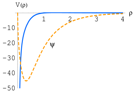
Figure 4: The potential (solid line) and the wave-function (dashed line) for the negative mode, obeying the equation $-d^{2}\psi/d\rho^{2}+V\,\psi=-k^{2}\psi$, for $d=5$.

3.2 Back-reaction

The back-reaction is comprised of the zero modes and of the second harmonic modes which we denote as

$$X^{(2)}(r,z)=\lambda^{2}\,x_{0}(r)+\lambda^{2}\,x_{2}(r)\cos(2\,k\,z),$$ (50)

where $X=A,B,C$ and $H$ (see also (38) ).

As usual, in the presence of compact space the modes having dependence along the internal dimensions decay exponentially with $r$ and they are massive in the Kaluza-Klein sense. The modes without $z$-dependence decay as inverse powers of $r$ and they are massless.

At any given order the gauge is given by (43). However, the gauge choice in higher orders can be modified by adding terms from the lower orders with the aim of simplifying the source terms.

Massless modes

Our method to simplify the equations is to choose the gauge such that the constraint $R_{rz}=0$ allows algebraic elimination of one of the fields. For the massless modes this constraint is trivially satisfied since these modes do not depend on $z$ (actually $R_{rz}$ is proportional to $k$ times the LHS of (42) after replacing the subscripts $1\to 0$). In this case for simplicity we adopt the same gauge as in (43)

$$b_{0}={2\,(d-2)\,f\,c_{0}+r\,f^{\prime}\,a_{0}\over 2\,(d-2)\,f+r\,f^{\prime}}.$$ (51)

Note that the variation of temperature at the horizon, which is proportional to $\exp(A-B)$, vanishes automatically in this gauge.

The equations governing the massless mode can be written schematically as

$$r^{-(d-2)}\left(r^{d-2}fh_{0}^{\prime}\right)^{\prime} = Src(a_{1},a_{1}^{\prime},h_{1},h_{1}^{\prime})$$

$${\cal E}_{a}(a_{0}^{\prime\prime},a_{0}^{\prime},c_{0}^{\prime},a_{0},c_{0}) = Src(a_{1},a_{1}^{\prime},h_{1},h_{1}^{\prime};h_{0},h_{0}^{\prime})$$

$${\cal E}_{c}(c_{0}^{\prime\prime},a_{0}^{\prime},c_{0}^{\prime},a_{0},c_{0}) = Src(a_{1},a_{1}^{\prime},h_{1},h_{1}^{\prime};h_{0},h_{0}^{\prime})$$

$${\cal Q}(a_{0}^{\prime},c_{0}^{\prime},a_{0},c_{0}) = Src(a_{1},a_{1}^{\prime},h_{1},h_{1}^{\prime};h_{0},h_{0}^{\prime}),$$ (52)

where the sources contain squared first order perturbations, the exact form of the operators ${\cal E}_{a},{\cal E}_{c},{\cal Q}$ and of the sources is found in Appendix A. The last equation is a constraint – it is not solved but we verify that it is satisfied by the solution of other equations in (3.2).

The equations (3.2) are subject to regularity boundary conditions at the horizon (A). These conditions determine the derivatives of the functions in terms of $a_{0}(1),c_{0}(1)$ and $h_{0}(1)$ which are 3 free parameters. At infinity we demand the length of the compact circle and the period of the Euclidean time to reach their unperturbed values, namely we demand that $A=H=0$ as $r\rightarrow\infty$. Besides, an obvious requirement is that $C$ approaches a constant at large $r$. However, it turns out that any choice of that constant yields regular solution to (3.2). In addition, the constraint is satisfied for any asymptotic value of $C$ and it does not contain any additional information beyond that already known from the second order equations. Therefore, we end up with $5$ out of $6$ conditions/parameters which are necessary to specify a unique solution to the three second order ODEs in (3.2).

The situation is puzzling only until one realizes that the choice (51) does not fix the gauge completely. By analyzing the residual gauge we find that fixing the residual reparameterization of $r$ is equivalent to choosing the asymptotic of $c_{0}$. To examine the effect consider a shift

$$r\rightarrow r+\xi(r),$$ (53)

that induces the variation in the metric functions:

$$\delta a_{0}={f^{\prime}\over 2\,f}\,\xi,~{}~{}~{}~{}~{}\delta c_{0}={\xi\over r},~{}~{}~{}~{}~{}\delta b_{0}=-{f^{\prime}\over 2\,f}\,\xi+\xi^{\prime},~{}~{}~{}~{}~{}\delta h_{0}=0.$$ (54)

Substituting this into (51), and demanding invariance of the gauge one gets a first order ODE for $\xi$. The equation has a solution such that $\xi(1)=0$ and that asymptotically $\xi=\xi_{\infty}\,r$, with some constant $\xi_{\infty}$. It follows from (54) that $\xi_{\infty}$ is the asymptotic value of $c_{0}$. Altogether we fix this remaining freedom by requiring $C=0$ at infinity.

To solve (3.2) we first treat $h_{0}$, which is decoupled from other metric functions. The solution is achieved in the “second shot hits” fashion since the equation contains only derivatives of $h_{0}$, similarly to what occurred at the first order. Then we solve two coupled equations for $a_{0}$ and $c_{0}$ where $h_{0}$ as well as squared first order perturbations act as sources. This is a two-parameter shooting problem: the values $c_{0}(1)$ and $a_{0}(1)$ are adjusted and the equations are integrated from the horizon outwards iteratively until a solution with asymptotically vanishing $a_{0}$ and $c_{0}$ is found. This completes the massless-modes computation.

Massive modes

The equations for these modes are similar to those we had at the linear order (45-47) but this time there are sources. To see if we need to modify the gauge (43) by adding some lower order terms squared we examine again the $R_{rz}=0$ equation:

$$2\,(d-2)\,f\,c_{2}+r\,f^{\prime}\,a_{2}+2\left(a_{2}^{\prime}+(d-2)c_{2}^{\prime}\right)+$$

$$+{d-1\over 2\,(d-2)}r\,f\,a_{1}\,a_{1}^{\prime}-\left(2\,(d-2)\,f+rf^{\prime}\right)b_{2}=0.$$ (55)

From here the obvious choice is

$$b_{2}={2\,(d-2)\,fc_{2}+rf^{\prime}a_{2}\over 2\,(d-2)\,f+r\,f^{\prime}}+{d-1\over 2\,(d-2)}{r\,f\,a_{1}\,a_{1}^{\prime}\over 2\,(d-2)\,f+r\,f^{\prime}},$$ (56)

since it allows algebraically to eliminate one of the fields, in precisely the same manner as at the linear order. Consequently, $c_{2}=-a_{2}/(d-2)$ and so we are left with only two second order ODEs to be solved.

Schematically, the equations read

$${\cal E}_{a}(a_{2}^{\prime\prime},a_{2}^{\prime},a_{2}) = Src(a_{1}^{\prime},a_{1},h_{1}^{\prime},h_{1}),$$

$${\cal E}_{h}(h_{2}^{\prime\prime},h_{2}^{\prime}) = Src(a_{1}^{\prime},a_{1},h_{1}^{\prime},h_{1};a_{2})$$ (57)

and their exact form is listed in (A). These equations are subject to regularity boundary conditions: both at the horizon, (A), and at infinity.

The $a_{2}$ equation is independent of $h_{2}$ and it is solved first. To this end we shoot with $a_{2}(1)$ as the shooting parameter. It is adjusted until the regular (decaying at large $r$) solution is found. The equation for $h_{2}$ contains $a_{2}$ as a source, see (3.2) or (A), and once $a_{2}$ is known $h_{2}$ is found by the “second shot hits” method. Finally, we verify that the constraint (A) is indeed satisfied by the solution.

3.3 Free energy and comparison with previous results

As soon as the negative mode and the resulting back-reaction are found we are ready to compute the coefficients of the free energy expansion about the critical point up to the fourth order in $\lambda$.

The quadratic term in the expansion (29), $F_{2}(X,X)$, is obtained by expanding the York-Gibbons-Hawking [16, 17] action integral (20) in our gauge. We find

$$I^{(2)} = -{\beta\,\Omega_{d-2}\over 16\pi G_{D}}\int_{0}^{L}dz\int_{r_{0}}^{\infty}dr\,r^{d-2}\,{d-1\over(d-2)}\cdot$$ (58)

$$\cdot\left[f\,\left({\partial}_{r}a(r,z)\right)^{2}+\left({\partial}_{z}a(r,z)\right)^{2}-{2(d-1)(d-3)\,f^{\prime 2}\over\left(2(d-2)f+r\,f^{\prime}\right)^{2}}\,a(r,z)^{2}\right]~{}.$$

Note that $h(r,z)$ does not appear here. To get $I^{(2)}$ in terms of harmonics $a_{n}(r)$, such as (41, 38) one needs only to substitute in the harmonic decomposition $a(r,z)=\sum_{n=0}^{\infty}a_{n}(r)\,\cos(n\,k\,z)$.

The quadratic part of the action (58) allows us to compute ${\cal A}$ (29). By definition the integrand vanishes for $k=k_{GL}$ and $a_{1}(r)$ being GL mode (found in subsection 3.1); the leading term appearing as one moves away from $k_{GL}$, reads

$$I^{(2)}=-{\beta\,\Omega_{d-2}\over 16\pi G_{D}}\int_{0}^{L}dz\int_{r_{0}}^{\infty}\left[2k_{GL}\delta k{d-1\over 2\,(d-2)}r^{d-2}a_{1}(r)^{2}\right]dr\lambda^{2},$$ (59)

Using the relations (1,7) and (8) we connect the dimensionless wavenumber with $\mu$ as $\delta k=2/(d-3)\delta\mu$. It follows then

$${\cal A}\equiv F^{(2)}/\lambda^{2}\propto{4\,\pi\,(d-1)\over(d-2)(d-3)}\int_{1}^{\infty}a_{1}^{2}\,r^{d-2}dr\ .$$ (60)

The factor of proportionality, $\Omega_{d-2}/(16\pi G_{D})$, appears in all action integrals such as (59). So in concrete calculations we shall get rid of it simply by suitably redefining the coefficients of the free energy expansion.

The quartic contribution to $F$ is (39). We omit the explicit expressions for the integrand of $F_{4GL}$ since it is far more cumbersome then (58,60), though it is straightforward to obtain. We note that in our gauge (43) $F_{4GL}$ includes pieces which originated in the metric function $B$ before the gauge was fixed.

The numerical values of ${\cal A}$ and of the specific terms forming ${\cal C}$ are listed in table 2. It is evident from this table that a critical dimension, $D^{*}_{can}=12.5$, for the canonical ensemble appears, above which ${\cal C}$ changes sign marking a change in the phase transition’s order.

d	4	5	6	7	8	9	10	11	12	13	14
${\mathbf{{\cal A}}}$	0.465	2.05	5.11	9.98	16.9	26.2	37.5	51.7	68.7	88.6	112
${\mathbf{{\cal C}}}$	-0.403	-1.39	-2.99	-5.03	-7.07	-8.47	-8.30	-5.27	1.97	15.0	35.7
$F_{4GL}$	.0976	.7883	3.035	8.417	19.27	38.85	71.42	122.48	198.8	308.8	462.2
$F_{2}(BR_{0})$	.3918	1.287	2.239	1.932	-2.112	-13.82	-38.86	-85.06	-162.4	-283.4	-463.3
$F_{2}(BR_{2})$	.1076	.8912	3.791	11.52	28.46	61.14	118.6	212.8	359.2	577.2	889.9

Table 2: Coefficients of the free energy expansions. We notice that ${\cal C}$ changes sign between $d=11$ and $12$. This indicates that in the canonical ensemble a second order phase transition occurs in dimensions $d\geq 12$.

There is a subtlety involved in the calculation of ${\cal C}$. According to (32) it is defined as a difference between two numbers, $F_{4GL}$ and $F_{2}(BR)$. As the dimension increases these numbers grow and they become comparable around $D^{*}_{can}$, see table 2. Hence, it is imperative to compute each term in (32) accurately enough in order to obtain reliable ${\cal C}$.

Having computed the coefficients in the free energy expansion we may obtain the micro-canonical thermodynamic coefficients $\eta_{1}$ and $\sigma_{2}$. These are defined in (14,18,2.2) and their numerical values are summarized in table 3. We include for comparison the same quantities computed in [3] (see also [4]) in Gubser’s method. We do not know which method is more accurate, but obviously both yield comparable results (with less than $5\%$ discrepancy.)

Landau-Ginzburg method, derived from ${\cal A},~{}{\cal C}$
d 4 5 6 7 8 9 10 11 12 13 14 $\eta_{1}$ 1.40 3.00 4.68 6.21 7.36 7.93 7.68 6.29 3.56 -0.695 -6.76 $\sigma_{2}$ -0.569 -0.976 -1.40 -1.79 -2.08 -2.21 -2.09 -1.70 -0.969 0.197 1.85

Previous method, direct computation
d 4 5 6 7 8 9 10 11 12 13 14 $\eta_{1}$ 1.45 3.03 4.69 6.21 7.34 7.89 7.66 6.25 3.57 -0.724 -6.84 $\sigma_{2}$ -0.595 -0.989 -1.42 -1.80 -2.02 -2.14 -2.08 -1.66 -0.966 0.198 1.82

Table 3: Coefficients of the dimensionless mass and of the entropy variation as defined in (18,2.2) computed in both the LG method and the previous method. The match is within $5\%$. The sign change (in both quantities) between $d=12$ and $d=13$ indicates a change in the order of the transition in the micro-canonical ensemble.

Notice that for each dimension both methods produce exactly two numbers that encode the entire thermodynamics at leading order: $\eta_{1}$ and $\sigma_{2}$ in the micro-canonical ensemble or ${\cal A}$ and ${\cal C}$ in the canonical ensemble, and we have demonstrated the relation between the two pairs of quantities. We note also that while in the canonical ensemble $\sigma_{1}=0$ automatically, in the micro-canonical ensemble this is a derived result. In fact, in that case the smallness of $\sigma_{1}$ can be used as an estimator of numerical error [2].

4 Several compact dimensions

After having demonstrated the LG-inspired method, we would like to apply it to the computation of the order of the transition in the presence of a more general compactification – by a torus.

Square torii. We choose to restrict our study to square torii, namely $z^{i}\sim z^{i}+L$ with the same $L$ for all $z^{i}$ and with right angles between the axes. We motivate this restriction by the following. We view the space of torii as having two boundaries – on the one hand highly asymmetrical torii, where one (or more) dimensions are much larger than the rest, and on the other hand highly symmetrical torii such as the square torus.

For example, for $p=2$ the space of torii is the well known modular domain parameterized by $\tau$. The highly asymmetrical 2-torus boundary is to be found at $\tau\to i\infty$. The most symmetrical torii, the square and hexagonal ones are to be found on the boundary at $\tau=i,\exp(i\,\pi/3)$ respectively. The boundary of the modular domain also includes other, less symmetrical torii. Actually, we could have chosen to study the hexagonal torus – it also enjoys a large symmetry that would simplify the calculations, and our choice is simply one of convenience.

The limit of highly asymmetrical torii is easy to understand. Suppose one of the edges of the torus is much longer than the rest (or equivalently, one of the vectors in the reciprocal torus is much shorter than others). In this case as the mass of the brane is reduced the first GL instability to occur will be associated with this long direction. Since this mode is invariant under translations in all other directions, and as long as that symmetry is not spontaneously broken (actually it may very well break to some extent during the collapse when the highest curvatures develop) then we find that we can completely ignore all directions except for the largest one. So effectively that case is reduced to that of a ${\bf T}^{1}$ compactification. A similar reduction applies if there are several directions which are much larger than the rest – in such a case we may reduce the problem to one with a smaller $p$.

Therefore by studying the limit of the symmetrical, square torus, we hope to achieve an understanding of both limits and thereby also some understanding of the intermediate region of general torii.

GL instability. In a ${\bf T}^{p}$ compactification (this discussion appeared already in [9]) we have a GL instability for each vector in the reciprocal lattice. This replaces the single instability and its harmonics in the ${\bf T}^{1}$ case. Therefore as the mass of the black brane is reduced these instabilities appear in order of smallness of the vectors in the reciprocal lattice. Of course, once the smallest one is encountered the system will start collapsing and we will not have a chance to observe the other instabilities separately.

For symmetrical torii, including the square, a non-generic phenomenon happens: as the first instability is reached (say by lowering the mass) several modes turn marginally tachyonic simultaneously. More precisely, for ${\bf T}^{p}$ there are $p$ such modes. One may be concerned that this degeneracy occurs only for exactly square torii, but we would like to argue that this degeneracy is relevant also for torii which are nearly square. Indeed, if the torus is not a precise square one of the GL instability modes will be triggered first. However, as the other “would be” tachyons have a very shallow potential at this moment, once the instability starts “rolling” and energy becomes available there is nothing to stop these modes from getting spontaneously excited, thereby allowing motion of the system in all the $p$ “tachyonic” directions just as for an exactly square torus.

Generalizing the perturbation method. We would now want to generalize the perturbation method and find a generalization for the coefficient ${\cal C}$ (32) which determines the order of the transition. The first order perturbation is an arbitrary linear combination of the $p$ GL modes, with coefficients denoted by $\lambda_{i}$, namely the generalization from $p=1$ to arbitrary $p$ is given by

$$X^{(1)}=\lambda\,X_{GL}\to X^{(1)}=\lambda_{i}\,X_{GL}^{i}~{},$$ (61)

where indices $i,j$ are to be summed in the range $1\leq i,j\leq p$ and $X_{GL}^{i}$ is the GL mode associated with $z^{i}$ (more explicitly, the mode computed in subsection 3.1 after substituting $z\to z^{i}$).

Proceeding to the second order the sources have the following schematic form $Src\sim\lambda_{i}\,\lambda_{j}\,X_{GL}^{i}\,X_{GL}^{j}$. Accordingly the back-reaction becomes

$$X_{BR}=\lambda_{i}\,\lambda_{j}\,X_{BR}^{ij}~{}.$$ (62)

To see the implications of the symmetries of the square on $X_{BR}^{ij}$, let us consider an arbitrary abstract tensor $T^{ij}$. Since the symmetries of the square allow us to exchange $z_{i}\leftrightarrow z_{j}$ for any $i$ and $j$ it is clear that there are only two independent components to $T^{ij}$ depending on whether $i=j$ or $i\neq j$, which we denote as $T^{=}$ and $T^{\neq}$ respectively. In summary

$$T^{ij}=\left\{\begin{array}[]{cc}T^{=}&~{}~{}~{}i=j\\ T^{\neq}&~{}~{}~{}i\neq j\end{array}\right.~{}.$$ (63)

We shall also make use of another definition, “T-average”

$$\bar{T}:={p\,T^{=}+p\,(p-1)\,T^{\neq}\over p^{2}}={T^{=}+(p-1)\,T^{\neq}\over p}$$ (64)

Thus there are two kinds of back-reaction. $BR^{=}$ is the one that was computed already for $p=1$, while $BR^{\neq}$ is novel and will be determined in the next section.

Now we must substitute the perturbation series

$$X=\lambda_{i}X_{GL}^{i}+\lambda_{i}\,\lambda_{j}\,X_{BR}^{ij}$$ (65)

into the action and compute the term of ${\cal O}(\lambda^{4})$. Concentrating on the quartic contribution of the GL modes we find the following generalization

$$F_{4GL}\,|\lambda|^{4}\to F_{4GL}^{ij}\,|\lambda_{i}|^{2}\,|\lambda_{j}|^{2}$$ (66)

($U(1)^{p}$ invariance requires the terms to have equal amounts of $\lambda^{i}$ and $\bar{\lambda}^{i}$). Similarly, the other factor in the ${\cal C}$ formula (32), $F_{2}(BR)$ gets generalized as

$$F_{2}(BR)\,|\lambda|^{4}\to F_{2}(BR^{ii},BR^{jj})\,|\lambda^{i}|^{2}\,|\lambda^{j}|^{2}+F_{2}(BR^{ij},BR^{ij})\,|\lambda^{i}|^{2}\,|\lambda^{j}|^{2}$$ (67)

(note that due to orthogonality of harmonics only the 0-harmonic contributes to $F_{2}(BR^{ii},BR^{jj})$ with $i\neq j$).

Altogether we find that ${\cal C}$ is replaced by a tensor

$${\cal C} \to {\cal C}(\lambda^{i})={\cal C}^{ij}\,|\lambda_{i}|^{2}\,|\lambda_{j}|^{2}$$

$${\cal C}^{ij} = \left\{\begin{array}[]{cc}{\cal C}^{=}&~{}~{}~{}i=j\\ {\cal C}^{\neq}&~{}~{}~{}i\neq j\end{array}\right.~{}.$$ (70)

Determination of the order. Consider ${\cal C}(\lambda^{i})$ as it varies over all possible directions in tachyon space $\lambda^{i}$. It is enough to consider unit vectors $\sum|\lambda_{i}|^{2}=1$, and thus the vector $|\lambda_{i}|^{2}$ varies over the simplex given by this normalization condition together the inequalities $0\leq|\lambda_{i}|^{2}$ (and $\leq 1$). We shall now show that the range of ${\cal C}(\lambda^{i})$ is precisely

$${\cal C}(\lambda^{i}) \in [{\cal C}^{=},\bar{\cal C}(p)]\subseteq[{\cal C}^{=},{\cal C}^{\neq}]$$ (71)

$$\bar{\cal C}(p) := {{\cal C}^{=}+(p-1)\,{\cal C}^{\neq}\over p}$$ (72)

where $[a,b]$ denotes here the interval between $a$ and $b$ irrespective of which one of $a,\,b$ is bigger. To see that we compute

$${\cal C}(\lambda^{i}) = {\cal C}^{ij}\,|\lambda_{i}|^{2}\,|\lambda_{j}|^{2}=$$ (73)

$$= {\cal C}^{=}\,\sum|\lambda_{i}|^{4}+{\cal C}^{\neq}\,\left(\left(\sum|\lambda_{i}|^{2}\right)^{2}-\sum|\lambda_{i}|^{4}\right)=$$

$$= {\cal C}^{\neq}+\left({\cal C}^{=}-{\cal C}^{\neq}\right)\sum|\lambda_{i}|^{4}~{}.$$

Since $\sum|\lambda_{i}|^{4}$ ranges precisely over $[1/p,1]$ (71) follows.

The transition is second order if and only if ${\cal C}(\lambda^{i})$ is positive for all directions in tachyon space $\lambda^{i}$, for otherwise, if there exists a vector $\lambda^{i}$ such that ${\cal C}(\lambda^{i})<0$ the system will spontaneously settle on that direction and a first order transition will ensue. We conclude that the transition is second order if and only if both

$${\cal C}^{=},\,\bar{\cal C}(p)\geq 0.$$ (74)

$p$-dependence from $p=2$. From their definition it is evident that ${\cal C}^{=},\,{\cal C}^{\neq}$ are $p$-independent. Actually ${\cal C}^{=}$ is already known from $p=1$

$${\cal C}^{=}={\cal C}$$ (75)

Moreover, it suffices to compute ${\cal C}^{\neq}$ for $p=2$ where the mixed $ij$ terms appear – the computation does not change for higher $p$.

Thus it remains to determine ${\cal C}^{\neq}$. Rather than determine it directly we take a somewhat more physical approach and pick the diagonal direction in $\lambda$ space, namely

$$\overline{\lambda_{i}}={1\over\sqrt{p}}\,\lambda$$ (76)

independently of $i$. ${\cal C}(\overline{\lambda_{i}})$ computed along this direction is precisely $\bar{\cal C}$ defined in (72). Therefore by computing $\bar{\cal C}|_{p=2}$ we obtain

$${\cal C}^{\neq}=2\,\bar{\cal C}|_{p=2}-{\cal C}^{=}~{}.$$ (77)

The ${\cal A}$ term in the free energy may be easily generalized as follows

$${\cal A}\,\delta\mu\,|\lambda|^{2}\to{\cal A}\,\delta\mu\,\lambda^{i}\,\bar{\lambda}^{i}~{},$$ (78)

and on the diagonal direction (76) $\bar{{\cal A}}={\cal A}$.

The actual computation (at $p=2$), which is fully described in the next section, requires obtaining the mixed term $F_{4GL}^{\neq}\,|\lambda_{1}|^{2}\,|\lambda_{2}|^{2}$ from substitution into the action, a new mixed term in $F_{2}(BR_{0})$, computing the mixed back-reaction term $BR^{\neq}\equiv BR_{11}$, which is in the $(\pm 1,\pm 1)$ harmonics, and finally substituting it into the quadratic action to obtain $F_{2}(BR_{11})$. All the other ingredients were essentially computed already for the $p=1$ case.

Micro-canonical ensemble. Having obtained the “diagonal” coefficients $\bar{{\cal C}}$ and $\bar{{\cal A}}$ we can compute the variation in dimensionless mass $\bar{\eta}$ (17) along this direction by using (18)

$$\bar{\eta}_{1}:=-2\,(d-3)\,{\bar{\cal C}\over\mu_{GL}\,{\cal A}}+{1\over d-2}\,\mu_{GL}{\cal A}$$ (79)

In fact, we can define a tensor of mass variation $\eta_{1}$, as in (64). Then, in analogy with what we had for the tensor ${\cal C}$, we have $\eta_{1}^{=}\equiv\eta_{1}|_{p=1}$, and recalling (77), $\eta_{1}^{\neq}=2\,\bar{\eta}_{1}|_{p=2}-\eta_{1}^{=}$. By analogy with (74) the transition will be second order in the canonical ensemble for a given $p$ exactly when both

$$\eta_{1}^{=},\bar{\eta}_{1}(p)<0~{},$$ (80)

where as before (72) we define $\bar{\eta}_{1}(p):=\eta_{1}^{=}/p+(p-1)\,\eta_{1}^{\neq}/p$.

5 Computation for ${\bf T}^{2}$

In this section we perform the computation for the square two-torus, so $D=d+p$ with $p=2$.

The most general metric consistent with the $U(1)_{t}\times SO(d-1)_{\Omega}$ isometries is

$$ds^{2}=f(r)\,e^{2\,A}dt^{2}+f(r)^{-1}\,e^{2\,B}dr^{2}+K_{i}\,dz^{i}\,dr+H_{i}\,dz^{i}dz^{i}+W\,dz^{1}dz^{2}+r^{2}\,e^{2\,C}d\Omega_{d-2}^{2}$$ (81)

where $i=1,2$. The metric in the $(r,\vec{z})$ space has $3$ gauge degrees of freedom. We fix $2$ of them by choosing $K_{i}=0$. The remaining degree of freedom will be fixed by considerations similar to the ${\bf T}^{1}$ case.

The square torus has also the following three discrete isometries, which will also be preserved by our perturbation

$$z_{1} \leftrightarrow z_{2}$$

$$z_{1} \to -z_{1}$$

$$z_{2} \to -z_{2}$$ (82)

First order – marginally tachyonic modes

In the square torus background two GL modes turn marginally tachyonic simultaneously, resulting in a two-dimensional “tachyon space”. In this section we focus on the diagonal direction in the “tachyon space”, given schematically by $\overline{\lambda_{i}}\,X_{GL}^{i}$ where

$$\overline{\lambda_{i}}=\lambda$$ (83)

Here it is convenient for us to use this normalization to compute the back-reaction and turn to the normalization (76), which differs by a $\sqrt{2}$ factor, later when we substitute into the free energy (which amounts to dividing the quadratic and the quartic coefficients of the free energy by $p=2$ and by $p^{2}=4$, respectively).

As in ${\bf T}^{1}$ case we use real $\lambda$. The diagonal instability is given explicitly in terms of the functions $a_{1}(r),\,b_{1}(r),\,c_{1}(r),\,h_{1}(r)$ and the critical constant $k\equiv k_{GL}$ which were found in subsection 3.1 as follows

$$X(r,z)=\lambda\,x_{1}(r)\,\sum_{i=1}^{2}\cos(k\,z_{i}),$$ (84)

for $X=A,B,C$ and

$$H_{i}(r,\vec{z}) = \lambda\,h_{1}(r)\cos(k\,z_{i}),$$

$$W = 0.$$ (85)

Clearly, because of the symmetry between the tachyons along the torus edges only a single function $h_{1}(r)$ is used for both $i$’s, and actually the relation $z_{1}\leftrightarrow z_{2}\Rightarrow H_{1}\leftrightarrow H_{2}$ will hold throughout the perturbation, so essentially the $H$’s reduce to a single function. Note that the discrete square symmetries (82) are indeed preserved by the perturbation.

As expected, after plugging the expansions into the Einstein equations, the equations for different $i$’s completely decouple. Besides, the gauge conditions and the equations are identical for every $i$ and they coincide with those derived in the ${\bf T}^{1}$ case, see (45-47). The upshot is that the first order computation in the ${\bf T}^{2}$ (${\bf T}^{p}$ in fact) case is essentially identical with ${\bf T}^{1}$.

Back-reaction

The form of the back-reaction sources can be roughly obtained by squaring the linear order expansions (84) and (5). In addition, a mixed $W$ term, which was absent in the ${\bf T}^{1}$ case, becomes possible.

Massless zero modes

The expansion here is essentially the same as for ${\bf T}^{1}$.

$$X(r,\vec{z}) = 2\,\lambda^{2}\,x_{0}(r)~{},$$

$$H_{1}=H_{2} = \lambda^{2}\,h_{0}(r)~{},$$

$$W = 0~{},$$ (86)

where $X=A,B,C$ and the $p=2$ factor comes from summing over the back-reaction zero-modes for all $i$. The vanishing of $W$ is dictated by the square symmetries (82).

To confirm this form we proceed as follows. We use the gauge (51). The ODEs obtained after substituting the above expansion into the Einstein equations are given by (A,A). The equations differ from the ${\bf T}^{1}$ case only by the appearance of the factor $p=2$ that multiplies the sources in (A). As a result, $h_{0}(r)$ is unchanged while $a_{0}$ and $c_{0}$ are modified – multiplied by $p=2$ relative to ${\bf T}^{1}$ solutions. Indeed, that was the reason that we introduced the factor of $2$ in (5).

Massive second harmonic modes

The treatment of these modes replicates the one we had for $p=1$. The obvious expansions

$$X(r,\vec{z})=\lambda^{2}\,x_{2}(r)\,\sum_{i=1}^{2}\cos(2k\,z_{i}),$$ (87)

for $X=A,B,C$ and

$$H_{i}(r,\vec{z}) = \lambda^{2}\,h_{2}(r)\cos(2\,k\,z_{i}),$$

$$W = 0,$$ (88)

yield exactly the same equations as for the one-torus (A). So nothing new needs to be solved.

Massive mixed modes

This is the longest section here, for these modes are the only new ones that were not discussed in the ${\bf T}^{1}$ section.

The only mixed modes expansions allowed by the symmetries (82) are

$$X(r,\vec{z})=\lambda^{2}\,x_{11}(r)\,\cos(k\,z_{1})\cos(k\,z_{2}),$$ (89)

for $X=A,B,C,H$ and

$$W(r,\vec{z})=\lambda^{2}\,w_{11}(r)\,\sin(k\,z_{1})\sin(k\,z_{2}).$$ (90)

Plugging this into the Einstein equations we examine the constraints $R_{rz_{i}}=0$ which take the form

$$b_{11} - \frac{2\,\left(d-2\right)\,c_{11}\,f+r\,a_{11}\,f^{\prime}}{2\,\left(d-2\right)\,f+r\,f^{\prime}}-\frac{2\,\left(d-1\right)}{d-2}\,\frac{r\,f\,a_{1}\,a_{1}^{\prime}}{\left[2\,\left(d-2\right)\,f+r\,f^{\prime}\right]}-$$ (91)

$$- \frac{2\,r\,f\,\left(2\,f-r\,f^{\prime}\right)\,a_{1}\,h_{1}^{\prime}}{{\left[2\,\left(d-2\right)\,f+r\,f^{\prime}\right]}^{2}}-\frac{f\,r\,\left[2\,h_{11}^{\prime}+w_{11}^{\prime}+2\,a_{11}^{\prime}+2\,(d-2)\,c_{11}^{\prime}\right]}{2\,\left(d-2\right)\,f+r\,f^{\prime}}=0.$$

As usual, this equation instructs us how to choose the gauge and we take

$$b_{11} = \frac{2\,\left(d-2\right)\,c_{11}\,f+r\,a_{11}\,f^{\prime}}{2\,\left(d-2\right)\,f+r\,f^{\prime}}+$$ (92)

$$+ \frac{2\,\left(d-1\right)\,r\,f\,a_{1}\,a_{1}^{\prime}}{\left(d-2\right)\,\left[2\,\left(d-2\right)\,f+r\,f^{\prime}\right]}+\frac{2\,r\,f\,\left(2\,f-r\,f^{\prime}\right)\,a_{1}\,h_{1}^{\prime}}{{\left[2\,\left(d-2\right)\,f+r\,f^{\prime}\right]}^{2}}.$$

This gauge is consistent with our basic choice (43) which at this order only gets modified by adding sources from lower orders.

Now (91) reduces to $2\,h_{11}^{\prime}+w_{11}^{\prime}+2\,a_{11}^{\prime}+2\,(d-2)\,c_{11}^{\prime}=0$ which we solve for $h_{11}$

$$h_{11}=-{1\over 2}\left[w_{11}+2\,a_{11}+2\,(d-2)\,c_{11}\right],$$ (93)

where the asymptotic boundary conditions are used to eliminate the integration constant.

The rest of the equations are given by (A). Their schematic form is

$${\cal E}_{a}(a_{11}^{\prime\prime},a_{11}^{\prime},c_{11}^{\prime},a_{11},c_{11}) = Src(a_{1},a_{1}^{\prime},h_{1},h_{1}^{\prime})$$

$${\cal E}_{c}(c_{11}^{\prime\prime},c_{11}^{\prime},a_{11}^{\prime},c_{11},a_{11}) = Src(a_{1},a_{1}^{\prime},h_{1},h_{1}^{\prime})$$

$$r^{-(d-2)}\left(r^{d-2}fw_{11}^{\prime}\right)^{\prime} = Src(a_{1},a_{1}^{\prime},h_{1}^{\prime};a_{11},c_{11}),$$ (94)

These equations are only partially coupled and can be further separated. The first two do not involve $w_{11}$ and moreover one gets a decoupled equation for $a_{11}-c_{11}$. Having solved it, we proceed to solve first for $a_{11}+c_{11}$ and then for $w_{11}$ where at each step earlier solutions appear as sources.

The equations are subject to the horizon boundary conditions (A) and asymptotically they must vanish. We shoot to solve the equations, and the values of the shooting parameters are given in table 7. Finally, the constraint (A) is verified to be satisfied.

Free energy and thermodynamics

In the rest of this section we change the normalization from (83) to (76).

The quadratic term in the free energy expansion remains unchanged relative to the ${\bf T}^{1}$ case: ${\cal A}_{p=2}=\bar{{\cal A}}={\cal A}_{p=1}$.

We turn to the quartic term

$$\bar{{\cal C}}=F_{4GL}-\left[F_{2}(BR_{0})+F_{2}(BR_{2})+F_{2}(BR_{11})\right]~{}.$$ (95)

We can figure out which additional terms appear in the zero mode contribution for ${\bf T}^{2}$ relative to ${\bf T}^{1}$

$$F_{2}(BR_{0})|_{p=2}=F_{2}(BR_{0})|_{p=1}-{1\over 2}\int_{1}^{\infty}r^{d-2}\,{h_{0}^{\prime}}^{2}dr.$$ (96)

The second harmonic contribution requires only a $p$-dependent factor (division by $p=2$)

$$F_{2}(BR_{2})|_{p=2}={1\over 2}F_{2}(BR_{2})|_{p=1}.$$ (97)

The mixed modes term, $F_{2}(BR_{11})$, is new, and likewise there is a new contribution to $F_{4GL}$. It is straightforward to substitute the expansions (89,90) into the action integral (remembering to divide by 4 due to change of normalization). The resulting expressions are cumbersome and not particularly illuminating; we omit their explicit form.

The numerical values of the various terms in (95) are recorded in table 4.

d	4	5	6	7	8	9	10	11	12	13	14
$\mathbf{\bar{{\cal C}}}$	-.441	-1.27	-2.28	-3.24	-3.76	-3.30	-1.23	3.17	10.9	23.2	40.6
$F_{4GL}$	.2869	2.403	9.864	28.97	69.59	145.9	277.5	489.4	813.9	1290	1967
$F_{2}(BR_{0})$	.2775	.8456	1.130	-0.2807	-5.992	-19.99	-48.14	-98.35	-180.7	-307.8	- 495.4
$F_{2}(BR_{11})$	.4023	2.377	9.121	26.76	65.24	30.57	59.29	478.2	804.0	1287	1977

Table 4: The non-trivial coefficients of the free energy expansions for ${\bf T}^{2}$. The rest of the coefficients are found using the fact that ${\cal A}$ is unchanged relative to ${\bf T}^{1}$ case, equation (97) and table 2.

d	4	5	6	7	8	9	10	11	12	13	14
$\bar{{\cal C}}_{p=2}$	-.441	-1.27	-2.28	-3.24	-3.76	-3.30	-1.23	3.17	10.9	23.2	40.6
${\cal C}^{=}$	-0.403	-1.39	-2.99	-5.03	-7.07	-8.47	-8.30	-5.27	1.97	15.0	35.7
${\cal C}^{\neq}$	-.481	-1.14	-1.57	-1.44	-.453	1.87	5.83	11.6	19.9	31.3	45.5

Table 5: Components of the tensor ${\cal C}$ (70), that determines the order of the phase transition in the canonical ensemble.

d	4	5	6	7	8	9	10	11	12	13	14
$\bar{\eta}_{1,p=2}$	1.49	2.81	3.89	4.65	5.02	4.84	3.99	2.40	-0.125	-3.73	-8.42
$\eta_{1}^{=}$	1.40	3.00	4.68	6.21	7.36	7.93	7.68	6.29	3.56	-0.695	-6.76
$\eta_{1}^{\neq}$	1.58	2.62	3.09	3.10	2.68	1.76	0.299	-1.48	-3.81	-6.77	-10.1

Table 6: Components of the tensor $\eta_{1}$ (17), that defines the dimensionless mass variation (see definition at the end of section 4) which determines the order of the phase transition in the micro-canonical ensemble.

$p$-dependence

Table 5 summarizes our results for the ${\cal C}$ tensor. For the various values of $d$, the number of extended dimensions, we give ${\cal C}\equiv{\cal C}^{=}$ which is the $p=1$ value, together with $\bar{{\cal C}}|_{p=2}$. From these we determine ${\cal C}^{\neq}$ using (77). ${\cal C}^{\neq}$ allows to extend the results to any $p$ by computing $\bar{\cal C}(p)$ from (72), which in turn determines the order of the transition in the canonical ensemble through (74).

For the micro-canonical ensemble ${\cal C}$ is replaced by the $\eta_{1}$ tensor, and table 6 summarizes the results, which were obtained through the use of (18,79). The condition for a second order transition is given in (80).

6 Discussion of implications

We demonstrated that the Landau-Ginzburg inspired method to compute the order is somewhat simpler than the previous one, and gives the same results (tables 2-3). In addition we analyzed the order of the Gregory-Laflamme transition for (square) torii compactifications. The main results are summarized in tables 4-6 and we now proceed to discuss their implications.

Transition order is independent of $p$. A necessary condition for a second order phase transition is $0<{\cal C}^{=}\equiv{\cal C}$ (74). Therefore, for all $D<D^{*}_{can}\equiv 12.5$, where the transition is first order for $p=1$ (namely ${\cal C}<0$) it is first order for all $p$.

From table 5 we find that the converse it true as well. For $d>D^{*}_{can}-1=11.5$ where ${\cal C}>0$ then also ${\cal C}^{\neq}>0$ and therefore from (72) also $\bar{\cal C}(p)>0$ for all $p$, and hence the transition is second order in this range of $d$ for all $p$.

Altogether we conclude that the transition order depends only on $d$, the number of extended dimensions, and not on $p$, the dimension of ${\bf T}^{p}$. It would be interesting to know whether this property holds for a general compactification manifold, $Y^{p}$.

Failure of the “equal-entropy for the equal-mass estimators”. Our original motivation for exploring the phase transition order in torus compactification arose after observing in [9] that the “equal entropy for equal mass” estimator indicates lower critical dimension for some higher-dimensional torii (lower then the $p=1$ value of $D^{*}=``13.5"$). In fact, this argument gave an encouraging value of “10” for ${\bf T}^{p}$ with $3\leq p\leq 6$. However, as just noted the critical dimension cannot be lowered, and here we explain why the estimator failed.

We shall now show that the estimator is strongly sensitive to the approximation error which is inherently built into it. In fact an approximation error in the percent and sub-percent level will even cancel the prediction of a critical dimension altogether. In other words, it turns out that the estimates of [9] carry unusually large error bars, which resolve the puzzle.

The estimator is constructed by comparing entropies of a uniform black-brane and of a localized black-hole with the same mass. The idea is that if entropy equality is achieved below the critical mass this may indicate that the phase transition between these objects is second order since a new non-uniform branch emerging from the GL point is likely to exist and to connect between the branches. The dimension (not necessarily integer) for which the “equal-entropy mass” coincides with the instability mass estimates the critical dimension. This is only an estimate because the entropy of a localized solution is approximated in this approach by a naive Schwarzschild value. This reasoning worked remarkably well in the ${\bf T}^{1}$ compactification [3], producing a fairly precise estimate of $D^{*}$.

However, the Schwarzschild formula is only an approximation to the localized black hole entropy, hence we use $S_{bh}(\eta)=S_{Schw}(\eta)(1+\epsilon)$, to model the modified expression. Perturbation theory [20, 21] and numerical results [22, 23] indicate that the entropy of a localized black hole is higher than that of a Schwarzschild black hole and hence we must take $\epsilon>0$.

Solving for $\eta$ we get

$$\eta_{S}(\epsilon)={1\over 16\,\pi}\left[{\Omega_{d-2}^{~{}D-3}\over\Omega_{D-2}^{~{}d-3}}{(d-2)^{(D-3)(d-2)}\over(D-2)^{(D-2)(d-3)}}\right]^{1/p}\,(1+\epsilon)^{(D-3)(d-3)/p}$$ (98)

To find the estimate for the critical dimension, $\tilde{D}^{*}$ we compare this with the critical mass, which is well approximated by the formula [3], $\eta_{c}(D,p)=\eta_{c}(D-p)=0.47\cdot 0.686^{D-p+1}$. Exploring the resulting dependence of this estimate on $\epsilon$ shows that $\tilde{D}^{*}$ increases fast as it grows. For example, in a $p=1$ case, while for $\epsilon=0$ one has $\tilde{D}^{*}\simeq 12.5$, taking $\epsilon=0.002$ results in $\tilde{D}^{*}\simeq 16$, and $\epsilon>0.003$ does not have a critical dimension at all. The situation is similar for other $p$’s and for $p=6$, $\epsilon\simeq 0.08$ sufficies to send $\tilde{D}^{*}\rightarrow\infty$.

In conclusion, there is no contradiction between our present results and the estimate due to the sensitivity of the latter to the actual value of the entropy of the localized phase.

Subtle spontaneous symmetry breaking. Examination of table 5 reveals that for all $d>4$ $\bar{\cal C}|_{p=2}>{\cal C}$ therefore the diagonal direction in tachyon space is disfavored relative to turning on a “single tachyon” namely a tachyon which depends only on a single $z^{i}$. We interpret that to mean that the discrete symmetries of the torus are spontaneously broken: for a first order decay the time evolution will proceed (at least initially) through a single tachyon, while for a second order transition the system will re-settle into a slightly non-uniform string where mostly a single tachyon is turned on. This makes sense if we recall that the square torus is a special torus, and for all nearly square torii the degeneracy of the GL modes is removed anyway (see section 4).

Micro-canonical ensemble. From table 6 we find that the behavior in the micro-canonical ensemble is similar to the case of the canonical ensemble (except for the known change in the critical dimension). Since $\eta_{1}^{\neq}<\eta_{1}^{=}$ for all $d>4$ in our table, then $\eta_{1}^{=}$ alone determines the order of the phase transition, and the order is independent of $p$ (for all $d$). Moreover, as discussed in the previous paragraph we conclude that a single tachyon is preferred over the diagonal direction through spontaneous symmetry breaking (for all $d>4$).

Acknowledgements

This research is supported in part by The Israel Science Foundation (grants no 228/02, 607/05) and by the Binational Science Foundation BSF-2002160, BSF-2004117. ES is supported in part by the Canadian Institute for Advanced Research Cosmology and Gravity Program and by the Natural Sciences and Engineering Research Council of Canada.

The authors are grateful to the KITP in Santa-Barbara where some final stages of this work took place. This research was supported in part by the National Science Foundation under Grant No. PHY99-07949.

Appendix A Second order perturbation equations

Here we give the full back-reaction equations for each harmonic, including the full expressions for the sources.

Zero-modes

First we solve the equation for $h_{0}$

$${1\over r^{d-2}}\left(r^{d-2}fh_{0}^{\prime}\right)^{\prime}=\left(\frac{k^{2}\,h_{1}}{2\,f}+\frac{2\,\left(d-1\right)\,\left(d-3\right)\,f^{\prime}\,a_{1}^{\prime}}{{\left[2\,\left(d-2\right)\,f+r\,f^{\prime}\right]}^{2}}\right)\frac{2\,f-r\,f^{\prime}}{2\,\left(d-2\right)\,f+r\,f^{\prime}}\,a_{1}-$$

$$\frac{4(d-1)^{2}(d-3)^{2}\,f^{\prime}}{{\left[2\,\left(d-2\right)\,f+r\,f^{\prime}\right]}^{4}}\,a_{1}^{2}-\frac{k^{2}\left[4(d-2)\,f\,\left[(d^{2}-3d+1)\,f+d\,r\,f^{\prime}\right]+r^{2}f^{\prime 2}\right]}{2\,(d-2)\,f{\left[2\,\left(d-2\right)\,f+r\,f^{\prime}\right]}^{2}}\,a_{1}^{2}.$$ (99)

Then the equations for $a_{0}$ and $c_{0}$ are solved

$$a_{0}^{\prime\prime}+\frac{2\,{\left(d-2\right)}^{2}\,f^{2}+4\,\left(d-2\right)\,r\,f\,f^{\prime}+r^{2}\,f^{\prime 2}}{r\,f\,\left[2\,\left(d-2\right)\,f+r\,f^{\prime}\right]}\,a_{0}^{\prime}+$$

$$\frac{\left(d-2\right)\,f^{\prime}\,\left[2\,\left(d-3\right)\,f+r\,f^{\prime}\right]}{2\,f\,\left[2\,\left(d-2\right)\,f+r\,f^{\prime}\right]}\,c_{0}^{\prime}+\frac{\left(d-2\right)\,\left(d-3\right)\,f^{\prime 2}}{f\,{\left[2\,\left(d-2\right)\,f+r\,f^{\prime}\right]}^{2}}\,(a_{0}-c_{0})=Src_{a_{0}},$$

$$c_{0}^{\prime\prime}+\frac{2\,(d-2)(2\,d-5)\,f^{2}+4\,(d-2)\,r\,f\,f^{\prime}+r^{2}\,f^{\prime 2}}{r\,f\,\left[2\,\left(d-2\right)\,f+r\,f^{\prime}\right]}\,c_{0}^{\prime}+\frac{2\,(d-2)}{r\,\left[2\,\left(d-2\right)\,f+r\,f^{\prime}\right]}\,a_{0}^{\prime}-$$

$$\frac{2\,\,f^{\prime}\,\left[(d-2)(d-3)\,{f}^{2}+\left(2\,d-5\right)\,r\,f\,f^{\prime}+r^{2}\,{f^{\prime}}^{2}\right]}{r\,f\,{\left[2\,\left(d-2\right)\,f+r\,f^{\prime}\right]}^{2}}(a_{0}-c_{0})=Src_{c_{0}},$$ (100)

where the sources are given by

$$Src_{a_{0}} = \frac{k^{2}\,\left(r\,f^{\prime}-2\,f\right)\,a_{1}^{2}}{2\,f\,\left[2\,\left(d-2\right)\,f+r\,f^{\prime}\right]}-\left[\frac{k^{2}\,h1}{2\,f}+\frac{2\,\left(d-1\right)\,\left(d-3\right)\,f^{\prime}\,{a_{1}}^{\prime}}{{\left[2\,\left(d-2\right)\,f+r\,f^{\prime}\right]}^{2}}\right]a_{1}-\frac{f^{\prime}\,h_{0}^{\prime}}{2\,f},$$ (101)

$$Src_{c_{0}} = \left[\frac{k^{2}\,h_{1}}{2\,(d-2)\,f}+\frac{2\,(d-1)\,(d-3)\,f^{\prime}\,{a_{1}}^{\prime}}{\left(d-2\right)\,{\left[2\,\left(d-2\right)\,f+r\,f^{\prime}\right]}^{2}}\right]a_{1}-\frac{h_{0}^{\prime}}{r}+$$ (102)

$$\frac{2\,(d-1)^{2}\,(d-3)\,f^{\prime 2}+(d-2)\,(2\,f-r\,f^{\prime})\,\left[2\,\left(d-2\right)\,f+r\,f^{\prime}\right]\,k^{2}}{2\,{\left(d-2\right)}^{2}\,f\,{\left[2\,\left(d-2\right)\,f+r\,f^{\prime}\right]}^{2}}\,a_{1}^{2}$$

The above equations are subject to regularity boundary conditions at the horizon

$$h_{0}^{\prime} = -{k^{2}\,a_{1}\,(a_{1}+(d-2)\,h_{1})\over 2\,(d-2)\,(d-3)},$$

$$a_{0}^{\prime} = -2\,(d-2)\,(a_{0}-c_{0})+{3\,k^{2}\,a_{1}\,(a_{1}-h_{1})\over 4\,(d-3)}-{(d-1)^{2}\,a_{1}^{2}+(d-2)\,h_{0}^{\prime}\over 2\,(d-2)},$$

$$c_{0}^{\prime} = 2\,(a_{0}-c_{0})-{k^{2}\,a_{1}\,(a_{1}-h_{1})\over 2\,(d-2)\,(d-3)}+{(d-1)^{2}\,a_{1}^{2}\over(d-2)^{2}},$$ (103)

where both the functions and their derivatives are evaluated at $r=r_{0}$. In addition, there is a constraint

$$2\,\left(d-2\right)\,f\,{a_{0}}^{\prime}+\left(d-2\right)\,{c_{0}}^{\prime}\,\left[2\,\left(d-3\right)\,f+r\,f^{\prime}\right]-$$

$$-\frac{2\,\left(d-3\right)\,\left(d-2\right)\,\left({a_{0}}-{c_{0}}\right)\,f^{\prime}}{2\,\left(d-2\right)\,f+r\,f^{\prime}}+\left(2\,\left(d-2\right)\,f+r\,f^{\prime}\right)\,{h_{0}}^{\prime}+$$

$$+\left(\frac{\left(d-1\right)\,k^{2}\,r}{2\,\left(d-2\right)}-\frac{\left(d-3\right)\,{\left(d-1\right)}^{2}\,r\,{f^{\prime}}^{2}}{\left(d-2\right)\,{\left(2\,\left(d-2\right)\,f+r\,f^{\prime}\right)}^{2}}\right){{a_{1}}}^{2}-\frac{\left(d-1\right)\,r\,f{a_{1}^{\prime}}^{2}}{2\,\left(d-2\right)}=0.$$ (104)

Second harmonic

The relevant equations are

$$f\,a_{2}^{\prime\prime}+\frac{(d-2)\,f+r\,f^{\prime}}{r}\,a_{2}^{\prime}+\left[-4\,k^{2}+\frac{2\,(d-1)(d-3)\,f^{\prime 2}}{{\left[2\,\left(d-2\right)\,f+r\,f^{\prime}\right]}^{2}}\right]a_{2}=Src_{a_{2}},$$

$${1\over r^{d-2}}\left(r^{d-2}fh_{2}^{\prime}\right)^{\prime}=Src_{h_{2}}.$$ (105)

The sources read

$$Src_{a_{2}} = -3\,\left[\frac{(d-1)(d-3)ff^{\prime}\,a_{1}^{\prime}}{\left[2\,\left(d-2\right)\,f+r\,f^{\prime}\right]^{2}}+{1\over 2}\,h_{1}\,k^{2}\right]\,a_{1}-$$

$$- \left[\frac{(d-1)^{2}\,(d-3)\,r\,f^{\prime 3}}{(d-2)\left[2\,\left(d-2\right)\,f+r\,f^{\prime}\right]^{3}}+\frac{3\,k^{2}\,(2\,f-r\,f^{\prime})}{2\,\left[2\,\left(d-2\right)\,f+r\,f^{\prime}\right]}\right]\,a_{1}^{2},$$

$$Src_{h_{2}} = \frac{2\,(d-1)\,(d-3)\,f\,f^{\prime}(2\,f-r\,f^{\prime})\,a_{1}^{\prime}\,a_{1}}{\left[2\,\left(d-2\right)\,f+r\,f^{\prime}\right]^{3}}-3\,(d-2)\,k^{2}\,h_{1}\,a_{1}+$$ (106)

$$+ \frac{4\,k^{2}\,(d-1)\,r\,f\,a_{1}^{\prime}}{\left[2\,\left(d-2\right)\,f+r\,f^{\prime}\right]}\,a_{1}+\frac{4\,(d-3)^{2}(d-1)^{2}f\,f^{\prime 2}}{\left[2\,\left(d-2\right)\,f+r\,f^{\prime}\right]^{4}}\,a_{1}^{2}+$$

$$- \left[\frac{k^{2}\left(4(d-2)f\left[(d^{2}-3\,d+5)\,f+(d-4)\,r\,f^{\prime}\right]+(4\,d-7)r^{2}f^{\prime 2}\right)}{\left[2\,\left(d-2\right)\,f+r\,f^{\prime}\right]^{2}}\right]\,a_{1}^{2}+$$

$$+ 4\,k^{2}\,\frac{2\,f-r\,f^{\prime}}{2\,\left(d-2\right)\,f+r\,f^{\prime}}\,a_{2}$$

These equations are subject to regularity boundary conditions at the horizon

$$a_{2}^{\prime} = -2\,\left(d-1-{2\,k^{2}\over d-3}\right)a_{2}+\left[{(d-1)^{2}\over d-2}-{3\,k^{2}\over 2\,(d-3)}\right]\,a_{1}^{2}+{3\,k^{2}\,a_{1}\,h_{1}\over 2\,(d-3)},$$

$$h_{2}^{\prime} = {8\,(d-2)\,a_{2}+a_{1}\,\left[(4\,d-7)a_{1}-3\,(d-2)\,h_{1}\right]\over 2\,(d-2)\,(d-3)}\,k^{2},$$ (107)

where both the functions and their derivatives are computed at $r=r_{0}$.

The constraint is

$$h_{2}^{\prime}+\frac{a_{2}^{\prime}\,\left(2\,f-r\,f^{\prime}\right)}{2\,\left(d-2\right)\,f+r\,f^{\prime}}+\frac{2\,\left(d-3\right)\,\left(d-1\right)\,f^{\prime}\,{a_{2}}}{{\left(2\,\left(d-2\right)\,f+r\,f^{\prime}\right)}^{2}}+$$

$$-\frac{\left(d-1\right)\,\left(d-3\right)\,f\,a_{1}\,a_{1}^{\prime}}{{\left(2\,\left(d-2\right)\,f+r\,f^{\prime}\right)}^{2}}-\frac{\left(d-1\right)\,r\,f\,{a_{1}^{\prime}}^{2}}{2\,\left(d-2\right)\,\left(2\,\left(d-2\right)\,f+r\,f^{\prime}\right)}-$$

$$-\left[\frac{\left(d-3\right)\,{\left(d-1\right)}^{2}\,r\,f^{\prime 2}}{\left(d-2\right)\,{\left(2\,\left(d-2\right)\,f+r\,f^{\prime}\right)}^{3}}+\frac{\left(d-1\right)\,k^{2}\,r}{2\,\left(d-2\right)\,\left(2\,\left(d-2\right)\,f+r\,f^{\prime}\right)}\right]\,a_{1}^{2}=0.$$ (108)

Mixed modes

The mixed modes back-reaction appears in the $\mathbf{T}^{p}$ calculation starting from $p=2$. The perturbations are governed by the equations

$$f\,a_{11}^{\prime\prime} + {(d-2)f+r\,f^{\prime}\over r}a_{11}^{\prime}-2\,k^{2}\,a_{11}+{2(d-2)(d-3)f^{\prime 2}\over\left[2\,(d-2)\,f+r\,f^{\prime}\right]^{2}}\,(a_{11}-c_{11})+Src_{a_{11}}=0,$$

$$f\,c_{11}^{\prime\prime} + {(d-2)f+r\,f^{\prime}\over r}c_{11}^{\prime}-2\,k^{2}\,c_{11}-{2(d-3)f^{\prime 2}\over\left[2\,(d-2)\,f+r\,f^{\prime}\right]^{2}}\,(a_{11}-c_{11})+Src_{c_{11}}=0,$$

$$f\,w_{11}^{\prime\prime} + {(d-2)f+r\,f^{\prime}\over r}w_{11}^{\prime}+Src_{w_{11}}=0.$$ (109)

where

$$Src_{a_{11}} = \frac{4(d-1)^{2}f^{\prime 2}\left(-2(d-3)(d-2)f^{2}-(d-1)rf^{\prime}f+r^{2}f^{\prime 2}\right)}{(d-2)\left(2(d-2)f+rf^{\prime}\right)^{3}}\,a_{1}^{2}+$$

$$+ \frac{k^{2}\left(4(d-2)f\left(8(d-2)^{2}f^{2}-\left(5d^{2}-27d+33\right)rf^{\prime}f-5(d-2)r^{2}f^{\prime 2}\right)\right)}{(d-2)\left(2(d-2)f+rf^{\prime}\right)^{3}}\,a_{1}^{2}-$$

$$- \frac{(4d-7)r^{3}f^{\prime 3}}{(d-2)\left(2(d-2)f+rf^{\prime}\right)^{3}}\,a_{1}^{2}+\frac{4(d-1)ff^{\prime}}{2(d-2)f+rf^{\prime}}\,a_{1}^{\prime}a_{1}+\frac{2f\left(2f-rf^{\prime}\right)}{2(d-2)f+rf^{\prime}}a_{1}^{\prime 2}+$$

$$+ \frac{2f\left(4(d-2)\left(2d^{2}-5d+1\right)f^{2}+\left(5d^{2}-6d-7\right)rf^{\prime}f-(d-3)r^{2}f^{\prime 2}\right)f^{\prime}}{\left(2(d-2)f+rf^{\prime}\right)^{3}}\,h_{1}^{\prime}a_{1}-$$

$$- \frac{rff^{\prime}}{2(d-2)f+rf^{\prime}}\,h_{1}^{\prime 2}+\frac{f\left(3r^{2}f^{\prime 2}+2f\left(4f(d-2)^{2}+(4d-9)rf^{\prime}\right)\right)}{\left(2(d-2)f+rf^{\prime}\right)^{2}}\,a_{1}^{\prime}h_{1}^{\prime},$$

$$Src_{c_{11}} = \frac{4(d-1)^{2}f^{\prime 2}\left(2(d-3)(d-2)f^{2}+(d-1)rf^{\prime}f-r^{2}f^{\prime 2}\right)}{(d-2)^{2}\left(2(d-2)f+rf^{\prime}\right)^{3}}\,a_{1}^{2}+$$

$$+ \frac{2k^{2}\left(2(d-2)r^{3}f^{\prime 3}+(2-d)\left(4(d-2)f^{2}\left(\left(d^{2}+d-7\right)f+(8-d)rf^{\prime}\right)\right)\right)}{(d-2)^{2}\left(2(d-2)f+rf^{\prime}\right)^{3}}\,a_{1}^{2}-$$

$$- \frac{(8d-21)r^{2}ff^{\prime 2}}{(d-2)^{2}\left(2(d-2)f+rf^{\prime}\right)^{3}}\,a_{1}^{2}-\frac{4(d-1)ff^{\prime}}{(d-2)\left(2(d-2)f+rf^{\prime}\right)}\,a_{1}^{\prime}a_{1}-$$

$$- \frac{4f\left((d-2)\left(5d^{2}-14d+5\right)f^{2}+4(d-2)drf^{\prime}f+r^{2}f^{\prime 2}\right)f^{\prime}}{(d-2)\left(2(d-2)f+rf^{\prime}\right)^{3}}\,h_{1}^{\prime}\,a_{1}-$$

$$- \frac{2f^{2}}{2(d-2)f+rf^{\prime}}\,h_{1}^{\prime 2}-\frac{2f\left(r^{2}f^{\prime 2}+(d-2)f\left(2(2d-3)f+3rf^{\prime}\right)\right)}{(d-2)\left(2(d-2)f+rf^{\prime}\right)^{2}}\,a_{1}^{\prime}h_{1}^{\prime}+$$

$$+ \frac{2f\left(rf^{\prime}-2f\right)}{(d-2)\left(2(d-2)f+rf^{\prime}\right)}\,a_{1}^{\prime 2},$$

$$Src_{w_{11}} = 2(d-2){c_{11}}\left(1+\frac{2f}{2(d-2)f+rf^{\prime}}\right)k^{2}+4{a_{11}}\left(1-\frac{(d-2)f}{2(d-2)f+rf^{\prime}}\right)k^{2}+$$ (110)

$$+ \frac{2\left[(2\,d-3)r^{2}\,f^{\prime 2}+4\,(d-2)\,f\left(\left[d^{2}-3\,d+3\right]\,f+(d-2)\,rf^{\prime}\right)\right]k^{2}}{(d-2)\left(2\,(d-2)\,f+rf^{\prime}\right)^{2}}\,a_{1}^{2}+$$

$$+ 4\left[\frac{(d-1)\,r\,f}{(d-2)\left(2\,(d-2)\,f+rf^{\prime}\right)}\,a_{1}^{\prime}\,a_{1}-\frac{r\,f\,\left(r\,f^{\prime}-2\,f\right)}{\left[2\,(d-2)\,f+r\,f^{\prime}\right]^{2}}\,h_{1}^{\prime}\,a_{1}\right]k^{2}.$$

The horizon boundary conditions for these equations are given by

$$a_{11}^{\prime} = \frac{\left[(4d-7)k^{2}-4(d-3)(d-1)^{2}\right]a_{1}^{2}+2(d-2)\left[\left(k^{2}-(d-5)d-6\right)a_{11}\right]}{(d-3)(d-2)}+c_{11},$$

$$c_{11}^{\prime} = \frac{2}{d-3}\,\left(\frac{2\left[(d-3)(d-1)^{2}-(d-2)k^{2}\right]a_{1}^{2}}{(d-2)^{2}}+\left(k^{2}-d+3\right)c_{11}\right)+a_{11},$$

$$w_{11}^{\prime} = -\frac{2\,k^{2}\left[(2\,d-3)\,a_{1}^{2}+(d-2)\,(2\,a_{11}+(d-2)\,c_{11})\right]}{(d-3)(d-2)}.$$ (111)

where the functions and the derivatives are evaluated at $r=r_{0}$.

Finally, the constraint for the mixed modes reads

$$w_{11}^{\prime}+\frac{2\left[(d-2)f+rf^{\prime}\right]a_{11}^{\prime}}{2(d-2)f+rf^{\prime}}+\frac{(d-2)\left[2(d-1)f+rf^{\prime}\right]c_{11}^{\prime}}{2(d-2)f+rf^{\prime}}+\frac{2(d-3)(d-2)f^{\prime}({a_{11}}-{c_{11}})}{\left(2(d-2)f+rf^{\prime}\right)^{2}}+$$

$$\frac{2(d-1)rf{a_{1}^{\prime}}^{2}}{(d-2)\left(2(d-2)f+rf^{\prime}\right)}+\frac{4(d-3)(d-1)fa_{1}a_{1}^{\prime}}{\left(2\,(d-2)f+rf^{\prime}\right)^{2}}-\frac{2rf{h_{1}^{\prime}}^{2}}{2(d-2)f+rf^{\prime}}-$$

$$\frac{4\,(d-2)f\left(-2(d-3)f^{2}+(d-5)rf^{\prime}f+r^{2}f^{\prime 2}\right)a_{1}h_{1}^{\prime}}{\left(2(d-2)f+rf^{\prime}\right)^{3}}+\frac{4(d-3)(d-1)^{2}rf^{\prime 2}a_{1}^{2}}{(d-2)\left(2(d-2)f+rf^{\prime}\right)^{3}}=0.$$ (112)

Appendix B Numerical issues and shooting parameters

In this appendix we give some details regarding our numerical implementation and describe several tests that demonstrate its robustness. In addition, we summarize the numerical values of the shooting parameters in table 7.

The ODEs encountered in this paper must be solved between the horizon and infinity, $r\in[r_{0},\infty)$. However, in practice we solve the equations only for $r\in[r_{0}+\epsilon,r_{max}]$, where $\epsilon\ll r_{0}$ and $r_{max}$ is some finite number. The first boundary is taken slightly outside $r_{0}$ because the equations become singular at the horizon. To get the correct boundary conditions at this point we Taylor-expand our functions to the third order about the horizon and find the expansion coefficients analytically by plugging the expansion into the equations. This enables us to compute the functions and their derivatives at $r_{min}=r_{0}+\epsilon$. We checked that the meaningful numbers cited in this paper are independent of $\epsilon$ (with better then $0.1\%$ precision) provided $\epsilon\leq 10^{-4}$. As for the outer boundary, its location is determined by the “empirical formula”, $r_{max}(d)\simeq 18-d$ in the range $4\leq d\leq 14$. Here too the meaningful numbers undergo less then $0.1\%$ variations when we tried larger $r_{max}$.

In our shooting routines we integrate the equations from $r_{min}$, where one of the boundary conditions (b.c.) is used, toward $r_{max}$ where we attempt to satisfy the asymptotic b.c. For $k\neq 0$ this integration will in general diverge when $r_{max}\rightarrow\infty$ since both the decaying and the growing solutions are present. Only for a specific value of the shooting parameter the growing solution is eliminated, the integration converges and asymptotic b.c. is satisfied. Our method to filter out this growing solution follows that of Gubser [2]: we use the integral of $|x(r)|^{2}$ near the outer boundary, where $x(r)$ is the mode we are solving for, as an indicator for how well the asymptotic b.c. is satisfied (for the true solution this integral must be negligible). The shooting and matching procedure is thus reduces to a minimization of that integral.

The situation is different for the zero modes, as for them a finite solution exists regardless of the value of the shooting parameters. In this case we demand that the solution vanishes asymptotically. This is easily accomplished for $h_{0}$, for whom “the second shot hits”. However, as described in section 3.2, the procedure should be iterated to make $a_{0}$ and $c_{0}$ vanish asymptotically. Moreover, because of the relatively slow power-law decay the location of the outer boundary at $r_{max}$, given by the above empirical formula, is insufficient to ensure this asymptotic vanishing accurately enough. So, in practice, after integrating the equations (A) to $r_{max}$ we set the sources to zero (since they decay exponentially and are already very small) and continue to integrate to some large $r_{asymp}$ (taken to be an order of magnitude larger than $r_{max}$.) In the vicinity of $r_{asymp}$ we fit the solutions by expressions of the form $a_{\infty}+\alpha/r^{d-2}$ and $c_{\infty}+\gamma/r^{d-2}$, which is the correct analytic behavior in the asymptotic region [18]. Then we compute $\Delta=|c_{\infty}|+|a_{\infty}|$, which is an effective measure for how well the boundary conditions are satisfied. To minimize $\Delta$ we iterate until $\Delta$ decreases below a certain tolerance.

The numerical values of all shooting parameters appearing in this paper are listed in table 7.

As soon as the solutions are obtained one must ensure that the constraints (47), (A), (A) and (A) are satisfied by these solutions. In our case we verified that the constraints are satisfied with better then $0.1\%$ precision. This together with other tests described above gives an idea of the numerical accuracy of our method.

d	4	5	6	7	8	9	10	11	12	13	14
$h_{1}(1)$	.434	.496	.532	.560	.576	.595	.604	.613	.620	.627	.631
$h_{0}(1)$	.796	1.01	1.24	1.48	1.73	1.96	2.21	2.46	2.71	2.95	3.21
$a_{0}(1)$	-.232	.015	.506	1.24	2.23	3.46	4.95	6.68	8.68	10.9	13.4
$c_{0}(1)$	-.730	-.921	-1.14	-1.38	-1.62	-1.86	-2.11	-2.36	-2.60	-2.85	-3.10
$a_{2}(1)$	-.40	.690	1.11	1.66	2.37	3.22	4.22	5.43	6.76	8.26	9.93
$h_{2}(1)$	-.812	-1.22	-1.65	-2.09	-2.54	-2.99	-3.46	-3.89	-4.38	-4.84	-5.47
$a_{11}(1)$	5.28	7.74	10.2	12.5	14.8	17.1	19.8	22.2	24.7	27.1	29.6
$c_{11}(1)$	-2.96	-2.92	-2.90	-2.88	-2.86	-2.84	-2.88	-2.89	-2.89	-2.90	-2.90
$w_{11}(1)$	2.96	4.01	5.04	6.04	7.03	8.01	9.08	10.1	11.0	12.1	13.1

Table 7: The shooting parameters in various dimensions. We assume here that the normalization for any $p$ is same as for ${\bf T}^{1}$. The last 3 lines appear only for torii ${\bf T}^{p}$ with $p\geq 2$.

References

- [1] R. Gregory and R. Laflamme, “Black Strings And P-Branes Are Unstable,” Phys. Rev. Lett. 70, 2837 (1993).
- [2] S. S. Gubser, “On non-uniform black branes,”, Class. Quant. Grav. 19, 4825 (2002).
- [3] E. Sorkin, “A critical dimension in the black-string phase transition,” Phys. Rev. Lett. 93, 031601 (2004) [arXiv:hep-th/0402216].
- [4] H. Kudoh and U. Miyamoto, “On non-uniform smeared black branes,” Class. Quant. Grav. 22, 3853 (2005) [arXiv:hep-th/0506019].
- [5] T. Harmark and N. A. Obers, “Black holes on cylinders,” JHEP 0205, 032 (2002).
- [6] B. Kol, “The phase transition between caged black holes and black strings: A review,” Phys. Rept. 422, 119 (2006) [arXiv:hep-th/0411240].
- [7] T. Harmark and N. A. Obers, “Phases of Kaluza-Klein black holes: A brief review,” arXiv:hep-th/0503020.
- [8] B. Kol, “Topology change in general relativity and the black-hole black-string transition,” JHEP 0510, 049 (2005) [arXiv:hep-th/0206220].
- [9] B. Kol and E. Sorkin, “On black-brane instability in an arbitrary dimension,” Class. Quant. Grav. 21, 4793 (2004) [arXiv:gr-qc/0407058].
- [10] R. C. Myers and M. J. Perry, “Black Holes In Higher Dimensional Space-Times,” Annals Phys. 172, 304 (1986).
- [11] L.D. Landau and E.M. Lifshitz , “Statistical Physics” part 1, Pergamon, 1993.
- [12] D. J. Gross, M. J. Perry and L. G. Yaffe, “Instability Of Flat Space At Finite Temperature,” Phys. Rev. D 25, 330 (1982).
- [13] H. S. Reall, “Classical and thermodynamic stability of black branes,” Phys. Rev. D 64, 044005 (2001).
- [14] T. Prestidge, “Dynamic and thermodynamic stability and negative modes in Schwarzschild-anti-de Sitter,” Phys. Rev. D 61, 084002 (2000) [arXiv:hep-th/9907163].
- [15] J. P. Gregory and S. F. Ross, “Stability and the negative mode for Schwarzschild in a finite cavity,” Phys. Rev. D 64, 124006 (2001).
- [16] J. W. York, “Role Of Conformal Three Geometry In The Dynamics Of Gravitation,” Phys. Rev. Lett. 28, 1082 (1972).
- [17] G. W. Gibbons and S. W. Hawking, “Action Integrals And Partition Functions In Quantum Gravity,” Phys. Rev. D 15, 2752 (1977).
- [18] B. Kol, E. Sorkin and T. Piran, “Caged black holes: Black holes in compactified spacetimes. I: Theory,” Phys. Rev. D 69, 064031 (2004) [arXiv:hep-th/0309190].
- [19] T. Harmark and N. A. Obers, “New phase diagram for black holes and strings on cylinders,” Class. Quant. Grav. 21, 1709 (2004) [arXiv:hep-th/0309116].
- [20] T. Harmark, “Small black holes on cylinders,” Phys. Rev. D 69, 104015 (2004) [arXiv:hep-th/0310259].
- [21] D. Gorbonos and B. Kol, “A dialogue of multipoles: Matched asymptotic expansion for caged black holes,” JHEP 0406, 053 (2004) [arXiv:hep-th/0406002].
- [22] E. Sorkin, B. Kol and T. Piran, “Caged black holes: Black holes in compactified spacetimes. II: 5D numerical implementation,” Phys. Rev. D 69, 064032 (2004) [arXiv:hep-th/0310096].
- [23] H. Kudoh and T. Wiseman, “Connecting black holes and black strings,” Phys. Rev. Lett. 94, 161102 (2005) [arXiv:hep-th/0409111].
- [24] D. Gorbonos, private communication.