SU(2) and SU(3) Yang-Mills thermodynamics and some implications

Abstract

We sketch the development of effective theories for SU(2) and SU(3) Yang-Mills thermodynamics. The most important results are quoted and some implications for particle physics and cosmology are discussed.

Received 30 March 2006Revised 24 November 2006

PACS Nos.: 11.15.Ex; 11.15.Tk; 12.40.Ee

1 Introduction

There are well-known reasons why the thermodynamics of Yang-Mills theories should be formulated in a rigorous, nonperturbative, and analytical setting: the nonconvergence of perturbative loop expansions owing (i) to its (at best) asymptotic nature [1] and (ii) to the weak screening of the magnetic sector (infrared instability) [2].

In 1975 Polyakov conjectured that the infrared instability of Yang-Mills theory can be cured by taking into account the spatial correlations provided by the topologically nontrivial sector [3]. Notice that the weight of a nontrivial, (anti)selfdual configuration in the partition function is of the form $\exp\left[-\frac{\mbox{const}}{g^{2}}\right]$ which has an essential singularity at $g=0$: A weak-coupling expansion thus ignores these configurations completely.

The purpose of this paper is to give a brief account of the development and of some implications of the effective theories for thermalized SU(2) and SU(3) Yang-Mills dynamics. The basic idea is to subject the dynamics of topological field configurations to an optimized spatial coarse-graining [4]. In this way the notion of dynamical ground states emerges which break the fundamental gauge symmetry in successive stages as temperature decreases. There are a deconfining, a preconfining, and a confining phase for SU(2) and SU(3) thermodynamics. The loop-expansion of thermodynamical quantities is nontrivial only in the deconfining phase. A two-loop calculation for the pressure seems to indicate a very rapid numerical convergence [5, 6]. Expanding in loops integrates out portions of quantum fluctuations which remain after the spatial coarse-graining. A fixed-order result predicts what should be regarded a quantum fluctuation in the next-order calculation. In the preconfining phase the excitations are free but massive dual gauge modes. A common characteristic of the deconfining and preconfining phases is that their ground-state pressures are negative: The dynamics of the ground state in each of these two phases generates vacuum-energy density which depends on temperature $T$ in a linear way. In the confining phase the ground-state pressure is precisely zero for $T\ll\Lambda$ where $\Lambda$ denotes the Yang-Mills scale. For $T\sim\Lambda$ thermal equilibrium sq down in the confining phase: The density of massive spin-1/2 fermion states (selfintersecting center-vortex loops) is over-exponentially rising with energy. By necessity this destroys the macroscopic homogeneity of the system (vicinity to a Hagedorn transition). We believe (but cannot prove at the present stage of development) that it is the physics taking place at the onsets of local Hagedorn transitions and the fact that the position of an intersection point in a center-vortex loop is a modulus of this soliton effectively lead to quantum mechanical transitions in any Standard-Model vertex involving charged particles.

The above-sketched results seem to resolve a number of problems both theoretical and empirical in nature. On the theoretical side, the infrared instability inherent in perturbative loop expansions is cured by an emerging adjoint Higgs mechanism after a spatial coarse-graining is performed over interacting calorons and anticalorons in the deconfining phase. The vanishing of the ground-state pressure in the confining phase is relevant for an understanding of the role of (naive) zero-point fluctuations in quantum field theories associated with nonabelian gauge symmetries. On the empirical side, there is a number of experimentally testable predictions arising from the postulate SU(2)${}_{\tiny\mbox{CMB}}\stackrel{{\scriptstyle\tiny\mbox{today}}}{{=}}U(1)_{Y}$. In the case of experimental confirmation of the latter the Standard Model’s mechanism for electroweak symmetry breaking is endangered by Big-Bang nucleosynthesis.

2 Deconfining phase

Here we gather the essential steps needed to construct the effective theory in the deconfining phase. Explaining some (and not all) technicalities, we resort to the case SU(2). Necessary generalizations to SU(3) are mentioned in passing.

To apply a spatial-coarse graining to the highly complex dynamics of a nonperturbative ground state at a high temperature $T\gg\Lambda$ one first writes a definition for the phase $\hat{\phi}$ of an adjoint scalar field $\phi$. In contrast to the (spatially homogeneous) modulus $|\phi|$ the phase $\hat{\phi}$ does not carry information on dimensional transmutation: in all admissible gauges it is periodic in the Euclidean time $\tau$. Therefore the derivation of its dynamics must involve exact solutions to the (Euclidean) equations of motion of the underlying theory. One can show that $\hat{\phi}$ is contained in the space of functions defined by the right-hand side of the following equation [4, 8]:

$$\hat{\phi}^{a}\equiv\frac{\phi^{a}}{|\phi|}(\tau)\sim\int d^{3}x\,\int d\rho\,\,\frac{\lambda^{a}}{2} F_{\mu\nu}[A_{\alpha}(\rho,\beta)]\left((\tau,0)\right)\,\left\{(\tau,0),(\tau,\vec{x})\right\}[A_{\alpha}(\rho,\beta)]\times$$

$$F_{\mu\nu}[A_{\alpha}(\rho,\beta)]\left((\tau,\vec{x})\right)\,\left\{(\tau,\vec{x}),(\tau,0)\right\}[A_{\alpha}(\rho,\beta)]\,.$$

In Eq. (2) a sum over trivial-holonomy calorons and anticalorons (in singular gauge) of topological charge modulus one is implicit, and the instanton scale parameter is denoted by $\rho$. The Wilson lines $\{(\tau,0),(\tau,\vec{x})\}=\{(\tau,\vec{x}),(\tau,0)\}^{\dagger}$ are to be performed along straight lines. When evaluating the right-hand side of Eq. (2) the only relevant term in the integrand is

$$2\,\frac{x^{a}}{r}\,\sin(2g(\tau,r))\frac{\partial_{r}^{2}\Pi(\tau,r)}{\beta r^{3}}$$ (2)

where $g\equiv\int_{0}^{1}ds\,\frac{r}{2}\partial_{\tau}\ln\Pi(t,sr)$, $\beta\equiv\frac{1}{T}$, $\Pi$ is the ‘pre’-potential of the (anti)caloron [7], $r\equiv|\vec{x}|$, and $a=1,2,3$. Since only spatial derivatives enter in (2) the nontriviality of $\hat{\phi}$ is associated with the magnetic sector of the theory. When evaluating the integral in Eq. (2) over the term in (2) ambiguities arise. On the one hand, the radial and the integration over $\rho$ diverge. On the other hand, the integration over the azimuthal angle yields a vanishing result. Regularizing all three integrals thus produces an undetermined normalization. The important point is that the angular regularization, which involves a particular direction $\hat{x}$ in space (breaking of rotational symmetry), is not gauge invariant: This would be overly restrictive. Rather, a change $\hat{x}\to\hat{x}^{\prime}$ boils down to a global gauge transformation. Since this does not affect the physics we conclude that the angular regularization employed is admissible. Moreover, one observes that the $\tau$ dependence of the integral in Eq. (2) (a sine subject to a phase shift) saturates very rapidly when increasing the cutoff for the $\rho$-integration to a few times $\beta=1/T$. To summarize, for given directions $\hat{x}_{C},\hat{x}_{A}$ (angular regularizations for caloron and anticaloron contribution) there are four parameters that are undetermined in the integral of Eq. (2): two phase shifts $\tau_{C}$ and $\tau_{A}$ and two normalizations $C_{C}$ and $C_{A}$ for the contributions of the caloron and the anticaloron, respectively [8]. Each set of ambiguities spans the kernel ${\cal K}$ of the linear differential operator ${\cal D}=\partial_{\tau}^{2}+\left(\frac{2\pi}{\beta}\right)^{2}$: The operator ${\cal D}$ thus is uniquely determined.

To find $\hat{\phi}$’s equation of motion one selects only those members of ${\cal K}$ which are BPS saturated, that is, energy- and pressure-free. (A spatial average over a noninteracting pair of energy- and pressure-free caloron and anticaloron (owing to their (anti)selfduality) needs to be energy- and pressure-free.) This is equivalent to $\hat{\phi}$ satisfying the following first-order equation: $\partial_{\tau}\hat{\phi}=\pm\frac{2\pi i}{\beta}{\hat{\lambda}}\,\hat{\phi}\,$ where $\hat{\lambda}$ is a normalized linear combination of the Pauli matrices $\lambda_{a}$. If, for definiteness, we set $\hat{\lambda}=\lambda_{3}$ then the solution to this equation of motion reads $\hat{\phi}=C\,\lambda_{1}\,\exp\left(\mp\frac{2\pi i}{\beta}\lambda_{3}(\tau-\tau_{0})\right)$. (The phase $\hat{\phi}$ winds along a circle on the group manifold $S_{3}$.) Thus the requirement of BPS saturation reduces the number of undetermined parameters from four to two: $C$ and $\tau_{0}$.

The modulus $|\phi|$ emerges because a Yang-Mills scale $\Lambda_{E}$ exists on the quantum level. At the same time, the length scale $|\phi|^{-1}$ determines the size of the volume over which the spatial coarse-graining, involving a caloron and its anticaloron, is performed. Still considering the interaction-free situation, a spatial coarse-graining down to the resolution $|\phi|$ yields an energy- and pressure-free field $\phi$: In the absence of interactions $\phi$ is BPS saturated. Since the right-hand side of $\phi$’s BPS equation defines the ‘square root’ of $\phi^{\prime}s$ potential $V_{E}(\phi)$ and since the spatial coarse-graining did not invoke an explicit $T$-dependence arising from the weight in the truncated partition function (recall, that the classical action of a caloron does not depend on $T$) the entire BPS equation must not exhibit an explicit $T$-dependence. Away from a phase transition, the ‘square root’ of $V_{E}$, in addition, should be an analytic function of $\phi$, and the known $\tau$-dependence of the phase $\hat{\phi}$ must be reproduced. Up to global gauge rotations the only viable possibility for $\phi$’s BPS equation then is:

$$\partial_{\tau}\phi=\pm i\,\Lambda_{E}^{3}\,\lambda_{3}\,\phi^{-1}\,$$ (3)

where $\phi^{-1}\equiv\frac{\phi}{|\phi|^{2}}$. Setting $C=1$ and substituting $\phi=|\phi|\hat{\phi}$ into Eq. (3), one has $|\phi|(\beta,\Lambda_{E})=\sqrt{\frac{\beta\Lambda_{E}^{3}}{2\pi}}$: The modulus $|\phi|$ falls off with the square root of increasing temperature. What is of great importance is that an action for the field $\phi$ follows from its BPS equation of motion and not vice versa. Namely, ‘squaring’ the right-hand side of Eq. (3), one arrives at $V_{E}=\mbox{tr}\frac{\Lambda_{E}^{6}}{\phi^{2}}=4\pi\Lambda_{E}^{3}T$. As a consequence, the usual freedom of shifting the potential, $V_{E}\to V_{E}+\mbox{const}$, allowed by the (second-order) Euler-Lagrange equations, is absent. Another important observation is that at a given temperature $T$ the mass squared $\partial^{2}_{|\phi|}\,V_{E}(|\phi|)$ of possible fluctuations $\delta\phi$ is much larger than the resolution squared $|\phi|^{2}$ and also than $T^{2}$. Thus $\phi$ is an inert background in the effective theory [4]: Quantum and statistical fluctuations $\delta\phi$ are absent! Both the classical and fluctuation inertness of $V_{E}(|\phi|)$ will lead to a uniquely determined energy density of the ground state.

After spatial coarse-graining the topologically trivial sector $\{a_{\mu}\}$ of the theory couples in a minimal way to the field $\phi$. In the effective action the kinetic term for $a_{\mu}$, $\frac{1}{4}\mbox{tr}\,G^{2}$ with $G_{\mu\nu}=\partial_{\mu}a_{\nu}-\partial_{\nu}a_{\mu}+ie[a_{\mu},a_{\nu}]$ and $e=e(T)$ being the effective gauge coupling, is that of the fundamental theory because of the latter’s renormalizability [9]. Namely, when expanded loop by loop in perturbation theory the kinetic term $\frac{1}{4}\mbox{tr}\,G^{2}$ is form invariant, that is, the effects of integrated-out quantum fluctuations solely reside in the momentum dependence of the gauge coupling and of the wave-function renormalization. Notice that the momentum that enters as an argument of the effective gauge coupling is given by the scale $|\phi|=|\phi|(T)$ down to which quantum fluctuations have been integrated out. The appearance of a wave-function renormalization translates into so-called compositeness constraints: if, in a physical gauge and for a given vertex, the momentum transfer is further off the mass-shell than the scale $|\phi|$ then this vertex does not exist in the effective theory. The issue of how strong the allowed interactions are in the effective theory was studied in [5, 6]: Interactions between (quasiparticle) excitations only contribute a fraction $\sim 10^{-3}$ to the total thermodynamical pressure (two-loop correction). We conjecture here that not much happens to the pressure beyond two-loops in the expansion in powers of $\hbar^{-1}$. One the one hand, this is suggestive because the compositeness constraints after the inclusion of the one-loop on-shell conditions become much tighter than on tree-level, probably so tight that at least a large fraction of all naively allowed diagrams does not exist beyond two-loop. On the other hand, there is an anti-weirdness argument. Beyond two-loops so-called pinch singularities take place. That is, one encounters expressions such as $\left(\delta(p^{2}-m^{2})\right)^{2}$ which, mathematically, make no sense at all. At least those diagrams that exhibit pinch singularities should be excluded by the (dressed) compositeness constraints. In a gauge theory the only classical zero-momentum gauge-field configuration is pure gauge, $G_{\mu\nu}=0$. Indeed, such a configuration $a_{\mu}^{bg}=\frac{\pi}{e}\,T\,\delta_{\mu 4}\lambda_{3}$ solves the gauge-field equation of motion

$$D_{\mu}G_{\mu\nu}=ie[\phi,D_{\nu}\phi]$$ (4)

of the effective theory. The configuration $a_{\mu}^{bg}$ represents, in an averaged way, all gluon exchanges of momentum transfer larger than $|\phi|$ in between calorons and anticalorons and radiative corrections thereof. The interesting feature is that $a_{\mu}^{bg}$ shifts the vanishing energy density $\rho^{gs}$ and the pressure $P^{gs}$ due to noninteracting calorons and anticalorons to finite values in the case of interactions: $\rho^{gs}=-P^{gs}=4\pi\Lambda_{E}^{3}T$. This renders the so-far hidden scale $\Lambda_{E}$ (gravitationally) detectable. A microscopic interpretation of this result is available [4, 8] owing to the work in [11, 12, 13, 14, 15].

It is useful to investigate the Polyakov loop ${\cal P}$ in the effective theory since performing a spatial coarse-graining and evaluating ${\cal P}$’s expectation are actions that essentially commute. In the gauge, where the field $\phi$ winds around the group manifold $S_{3}$, one has: ${\cal P}[a_{\mu}^{bg}=\frac{\pi}{e}\,T\delta_{\mu 4}\,\lambda_{3}]=-{\bf 1}$. In unitary gauge, which is reached by an admissible albeit singular gauge transformation [4], one obtains: ${\cal P}[a_{\mu}^{bg}=0]={\bf 1}$. As a consequence, the ground state is degenerate w.r.t. an electric $Z_{2}$ symmetry. This statement remains valid on the level of the total expectation $\left\langle{\cal P}\right\rangle$ because the field $\phi$ breaks the gauge symmetry as SU(2)$\to$U(1) thus saving the masslessness of one color direction. We conclude that the discussed phase is, indeed, deconfining. For SU(3) one obtains an adjoint scalar field $\phi$ which winds in each of the (not entirely independent) SU(2) subalgebras for a third of the time $0\leq\tau\leq\beta$. The Polyakov-loop expectation now is degenerate w.r.t. a $Z_{3}$ electric symmetry, and two directions in color space remain massless. For SU(N) with $N\geq 4$ no unique phase diagram exists with the possible exception of $N=\infty$.

Let us now briefly describe the physics of excitations. By the adjoint Higgs mechanism and in unitary gauge $\phi=\mbox{const},a^{bg}_{\mu}=0$ two (six) out of three (eight) color direction acquire a mass for SU(2) (SU(3)): Gluons become thermal quasiparticle excitations on tree-level by coarse-grained interactions with the ground state. For SU(2) one has $m=2e|\phi|$, for SU(3) $m_{2}=2e|\phi|$ and $m_{4}=e|\phi|$. Massive gauge bosons provide for infrared cutoffs and thus cure the old perturbative instability problem of the magnetic sector. To learn how the effective gauge coupling $e$ depends on the cutoff $|\phi|$ (and thus on temperature $T$) one imposes the requirement that the pressure and energy density are related by one and the same Legendre transformation, regardless of whether one chooses to calculate them in fundamental or effective field variables. On the level of free quasiparticles, which is sufficient for many practical situations, one arrives at the following evolution equation: $\partial_{a}\lambda_{E}=-\frac{24\lambda_{E}^{4}a}{(2\pi)^{6}}\frac{D(2a)}{1+\frac{24\lambda_{E}^{3}a^{2}}{(2\pi)^{6}}}$ where $\lambda_{E}\equiv\frac{2\pi T}{\Lambda_{E}}$, $a\equiv\frac{m}{2T}$, and $D(a)\equiv\int_{0}^{\infty}dx\,\frac{x^{2}}{\sqrt{x^{2}+a^{2}}}\,\frac{1}{\exp(\sqrt{x^{2}+a^{2}})-1}\,$. Notice that $e$, $\lambda$, and $a$ are related as: $a=2\pi\,e\,\lambda_{E}^{-3/2}\,$. As a result of the one-loop evolution, $e$ is essentially constant for $\lambda_{E}$ sufficiently larger than $\lambda_{c,E}$. One has $e=8.89,\,\lambda_{c,E}=13.87$ (SU(2)) and $e=7.26,\,\lambda_{c,E}=9.475$ (SU(3)). For $\lambda_{E}\searrow\lambda_{c,E}$ the coupling diverges in a logarithmic fashion: $e\sim-\log(\lambda_{E}-\lambda_{c,E})$. As a consequence, stable and screened magnetic monopoles, which are isolated objects deep inside the preconfining phase[4, 15], become massless at $\lambda_{c,E}$ and thus condense. The associated phase transition is second-order like [4]. It is worth mentioning that the entire thermodynamics of the deconfining phase is robust against changes of initial conditions set at a sufficiently high temperature: A decoupling of ultraviolet from infrared physics takes place. To set $m=0$ for $T>T_{i}\gg T_{c,E}$, where $m(T_{i})=0$ is the initial condition for the (downward) evolution of the effective coupling $e$, and to still believe in the physical relevance of four-dimensional Yang-Mills gauge-field theory is a contradiction: As we have learned, even at a high temperature this dynamics is only consistent nonperturbatively. We thus conclude that $T_{i}$ must coincide with the temperature where the concept of a four-dimensional, smooth spacetime manifold breaks down. There are good reasons to believe that $T_{i}\sim 1.2\times 10^{19}\,$GeV.

3 Preconfining phase

Let us know discuss what happens at and slightly below $T_{c,E}$. Because of total screening, magnetic monopoles (one species for SU(2), two species for SU(3)) become massless, and thus are extremely abundant: All memory of the existence of the Yang-Mills scale $\Lambda$ is washed away at $T_{c,E}$. The theoretical challenge is to describe the associated, newly emerging ground-state physics in an analytical way. It is clear that due to the highly complex dynamical situation exact results, again, require the process of a spatial coarse-graining.

The situation in the case of SU(2) is the following: The key is to consider the mean magnetic flux $\bar{F}_{\pm,\tiny\mbox{thermal}}$ of a noninteracting monopole-antimonopole pair of vanishing spatial momentum (also for each constituent) through an $S_{2}$ of infinite radius in a thermal environment. (A finite radius would be associated with a mass scale which does not yet exist.) One has

$$\bar{F}_{\pm,\tiny\mbox{thermal}}(\delta) = \,4\pi\,\int d^{3}p\,\delta^{(3)}(\vec{p})\,n_{B}(\beta|E(\vec{p})|)\,\bar{F}_{\pm}$$ (5)

$$= \pm\frac{8\pi\,\delta}{e}\int d^{3}p\,\frac{\delta^{(3)}(\vec{p})}{\exp\left[\beta\sqrt{M_{m+a}^{2}+\vec{p}^{2}}\right]-1}\,$$

where $\bar{F}_{\pm}\equiv\pm\frac{\delta}{2\pi}\frac{4\pi}{e}=\pm\frac{2\delta}{e}$, and $\delta\,,\ \ (0\leq\delta\leq\pi),$ is the angle between the Dirac strings of the monopole and antimonopole. (We work in unitary gauge on the microscopic level.) After setting $\vec{p}=0$ (spatial average) in $\left(\exp\left[\beta\sqrt{M_{a+b}^{2}+\vec{p}^{2}}\right]-1\right)$ and with $M_{a+b}=\frac{8\pi^{2}}{e\beta}$ (after screening [12, 13, 14]), the expansion of this term reads

$$\lim_{\vec{p}\to 0}\left(\exp\left[\beta\sqrt{M_{m+a}^{2}+\vec{p}^{2}}\right]-1\right)=\frac{8\pi^{2}}{e}\left(1+\frac{1}{2}\frac{8\pi^{2}}{e}+\frac{1}{6}\left(\frac{8\pi^{2}}{e}\right)^{2}+\cdots\right)\,.$$ (6)

The limit $e\to\infty$ can safely be performed in Eq. (5), and we have

$$\lim_{e\to\infty}\bar{F}_{\pm,\tiny\mbox{thermal}}(\delta)=\pm\frac{\delta}{\pi}\,,\ \ \ \ \ \ (0\leq\delta\leq\pi)\,.$$ (7)

This is finite and depends on the angular variable $\delta$ continuously. Now $\frac{\delta}{\pi}$ is a (normalized) angular variable just like $\frac{\tau}{\beta}$ is. Thus we may set $\frac{\delta}{\pi}=\frac{\tau}{\beta}$. The macroscopic complex field $\varphi$, describing the monopole condensate in the absence of interactions, is spatially homogeneous and its phase $\hat{\varphi}\equiv\frac{\varphi}{|\varphi|}$ depends on $\frac{\tau}{\beta}$ only and in a periodic way. Moreover, since the physical flux situation for the thermalized monopole-antimonopole pair does not repeat itself for $0\leq\frac{\delta}{\pi}\leq 1$ we conclude that this period is $\pm$ unity:

$$\hat{\varphi}(\tau)=C\exp\left[\pm 2\pi i\frac{\tau-\tau_{0}}{\beta}\right]\,$$ (8)

where $C$ and $\tau_{0}$ are undetermined.

To derive $\varphi$’s modulus, which together with $T$ determines the length scale $|\varphi|^{-1}$ over which the spatial average is performed, we proceed in close analogy to the deconfining phase. That is, we assume the existence of an (at this stage) externally provided mass scale $\Lambda_{M}$. Since the weight for integrating out massless and noninteracting monopole-antimonopole systems in the partition function is $T$ independent and since the cutoff in length for the spatial average defining $|\varphi|$ is $|\varphi|^{-1}$, an explicit $T$ dependence ought not arise in any quantity being derived from such a coarse-graining. That is, in the effective action density any $T$ dependence (still assuming the absence of interactions between massless monopoles and antimonopoles when performing the coarse-graining) must appear through $\varphi$ only. Moreover, integrating massless and momentum-free monopoles and antimonopoles into the field $\varphi$ means that this field is energy- and pressure-free: $\varphi$’s $\tau$ dependence (residing in its phase) must be BPS saturated. On the right-hand side of $\varphi$’s or $\bar{\varphi}$’s ($\varphi$’s complex conjugate) BPS equation the requirement of analyticity (because away from a phase transition the monopole condensate should exhibit a smooth $T$ dependence) and linearity in $\varphi$ or $\bar{\varphi}$ (because the $\tau$ dependence of $\varphi$’s phase, see Eq. (8), needs to honoured) yields the following first-order equation of motion

$$\partial_{\tau}\varphi=\pm i\frac{\Lambda_{M}^{3}\,\varphi}{|\varphi|^{2}}=\pm i\frac{\Lambda_{M}^{3}}{\bar{\varphi}}\,.$$ (9)

Substituting $\varphi=|\varphi|\hat{\varphi}$ into Eq. (9) and appealing to Eq. (8) (setting $C=1$), we derive $|\varphi|=\sqrt{\frac{\Lambda_{M}^{3}\beta}{2\pi}}$. Notice that the ‘square’ of the right-hand side in Eq. (9) uniquely defines $\varphi$’s potential $V_{M}$. (In contrast to a second-order equation of motion, following from an action by means of the variational principle, Eq. (9) does not allow for a shift $V_{M}\to V_{M}+\mbox{const}$.) For the case SU(3) the BPS equation (9) emerges for each of the two independent monopole condensates $\varphi_{1}$ and $\varphi_{2}$.

Again, by comparing the curvature of their potentials with the square of temperature and the squares of their moduli, one concludes that that the field $\varphi$ (SU(2)) and the fields $\varphi_{1}$, $\varphi_{2}$ (SU(3)) neither fluctuate on-shell nor off-shell[4]: Spatial coarse-graining over nonfluctuating, classical configurations generates inert macroscopic fields.

To derive the full effective theory the spatially coarse-grained and topologically trivial (dual) gauge fields $a^{D}_{\mu}$ (SU(2)) and $a^{D}_{\mu,1}$, $a^{D}_{\mu,2}$ (SU(3)) are minimally coupled (with a universal effective magnetic coupling $g$) to the inert fields $\varphi$ (SU(2)) and $\varphi_{1}$, $\varphi_{2}$ (SU(3)). The kinetic terms for $a^{D}_{\mu}$ (SU(2)) and $a^{D}_{\mu,1}$, $a^{D}_{\mu,2}$ (SU(3)) are canonical. Since the effective theory is abelian with (spontaneously broken) gauge group U(1)_D (SU(2)) and U(1)${}^{2}_{D}$ (SU(3)) and since the monopole fields do not fluctuate it follows that thermodynamical quantities are exact on the one-loop level. Before we discuss the spectrum of quasiparticles running in the loop we need to derive the full ground-state dynamics in the effective theory. The classical equations of motion for the dual gauge field $a^{D}_{\mu}$ are

$$\partial_{\mu}G^{D}_{\mu\nu}=ig\left[\overline{{\cal D}_{\nu}\varphi}\varphi-\bar{\varphi}{\cal D}_{\nu}\varphi\right]$$ (10)

where $G^{D}_{\mu\nu}=\partial_{\mu}a^{D}_{\nu}-\partial_{\nu}a^{D}_{\mu}$ and ${\cal D}_{\mu}\equiv\partial_{\mu}+ig\,a^{D}_{\mu}$. (For SU(3) the right-hand sides for the two equations for the dual gauge fields $a^{D}_{\mu,1}$, $a^{D}_{\mu,2}$ can be obtained by the substitutions $\varphi\to\varphi_{1}$ or $\varphi\to\varphi_{2}$ in Eq. 10.) The pure-gauge solution to Eq. (10) with ${\cal D}_{\mu}\varphi\equiv 0$ is given as $a^{D,bg}_{\mu}=\pm\delta_{\mu 4}\frac{2\pi}{g\beta}$. In analogy to the deconfining phase, the coarse-grained manifestation $a^{D,bg}_{\mu}$ of monopole-antimonopole interactions, mediated by dual, off-shell plane-wave modes on the microscopic level, shifts the energy density $\rho^{gs}$ and the pressure $P^{gs}$ of the ground state from zero to finite values: $\rho^{gs}=-P^{gs}=\pi\,\Lambda_{M}^{3}\,T$ (SU(2)) and $\rho^{gs}=-P^{gs}=2\pi\,\Lambda_{M}^{3}\,T$ (SU(3)).

In contrast to the deconfining phase, where $P^{gs}<0$ arises from monopole-antimonopole attraction, the negative ground-state pressure in the preconfining phase originates from collapsing and re-created center-vortex loops [4]. (There are two species of such loops for SU(3) and one species for SU(2)). The core of a given center-vortex loop can be pictured as a stream of the associated monopole species flowing oppositely directed to the stream of their antimonopoles [16]. Since by Stoke’s theorem the magnetic flux carried by the vortex is determined by the dual gauge field $a^{D,\tiny\mbox{tr}}_{\mu}$ transverse to the vortex-tangential and since $a^{D,\tiny\mbox{tr}}_{\mu}$ is – in a covariant gauge – invariant under collective boosts of the streaming monopoles or antimonopoles in the vortex core it follows that the magnetic flux solely depends on the monopole charge and not on the collective state of monopole-antimonopole motion. This, in turn, implies a center-element classification of the magnetic fluxes carried by the vortices justifying the name center-vortex loop. Viewed on the level of large-holonomy calorons an unstable center-vortex loop is created within a region where the mean axis for the dissociation of several calorons represents a net direction for the monopole-antimonopole flow. Notice that each so-generated vortex core must form a closed loop due to the absence of isolated magnetic charges within the monopole condensate. In contrast to the deconfining phase a rotation to (macroscopic) unitary gauge $a^{D,bg}_{\mu}=0,\varphi=|\varphi|$ is facilitated by a smooth, periodic gauge transformation which leaves the value ${\bf 1}$ of the Polyakov loop invariant: The electric $Z_{2}$ degeneracy, observed in the deconfining phase, is lifted in the ground-state. (For SU(3) it is an electric $Z_{3}$ degeneracy that is lifted.) By the dual (abelian) Higgs mechanism the mass of (noninteracting) quasiparticle modes is given as: $m=g|\varphi|$ (SU(2)) and $m_{1}=g|\varphi_{1}|=g|\varphi_{2}|=m_{2}$ (SU(3)).

The evolution of the effective magnetic coupling $g$ is determined (for both SU(2) and SU(3)) by the equation $\partial_{a}\lambda_{M}=-\frac{12\lambda_{M}^{4}a}{(2\pi)^{6}}\frac{D(a)}{1+\frac{12\lambda_{M}^{3}a^{2}}{(2\pi)^{6}}D(a)}$ where $\lambda_{M}\equiv\frac{2\pi T}{\Lambda_{M}}$, $a\equiv\frac{m}{T}$, and $a=2\pi g\lambda_{M}^{-3/2}$. Continuity of the pressure at $T_{c,E}$ relates the scales $\Lambda_{M}$ and $\Lambda_{E}$ as: $\Lambda_{E}\sim(1/4)^{1/3}\Lambda_{M}$ for SU(2) and $\Lambda_{E}\sim(1/2)^{1/3}\Lambda_{M}$ for SU(3). The coupling $g$ rapidly rises from zero at $\lambda_{c,E}$ (corresponding to $\lambda_{M}=8.478$ (SU(2)) and $\lambda_{M}=7.376$ (SU(3))) to infinity at $\lambda_{c,M}=7.075$ (SU(2)) and at $\lambda_{c,M}=6.467$ (SU(3)): $g\sim-\log(\lambda_{M}-\lambda_{c,M})$. We conclude that the preconfining phase occupies only a narrow region in the phase diagram of each theory. At $\lambda_{c,M}$ the core of a center vortex loop exhibits a vanishing diameter, and the pressure outside of the core vanishes: Single center-vortex loops become massless and stable spin-1/2 excitations.

4 Confining phase

Here were are interested in the physics taking place below $T_{c,M}$. At $T_{c,M}$ single center-vortex loops are extremely abundant: They conspire to form a newly emerging ground state subject to complex internal dynamics. To derive the dynamics of a macroscopic, complex field $\Phi$ describing this situation, again, a spatial coarse-graining is needed.

In the absence of interactions between center-vortex loops (only contact interactions are possible due to the decoupling of the dual gauge modes at $T_{c,M}$) the phase of this field is determined by the quantum statistical average flux through an $S_{1}$ of infinite radius, centered at the spatial point $\vec{x}$.

At $T_{c,M}$ the average flux due to a system $S$ of a center-vortex loop and its flux-reversed partner, both at rest, reads

$$\lim_{g\to\infty}\,F_{\tiny\mbox{thermal}} = 4\pi F\,\int d^{3}p\,\,\delta^{(3)}(\vec{p})\,n_{B}(\beta|2\,E_{v}(\vec{p})|)$$ (11)

$$= 0,\pm\frac{8\pi}{\beta|\varphi|}=0,\pm 4\,\lambda^{3/2}_{c,M}\,$$

where $F$ is (the vanishing) flux of the system when not coupled to the heat bath. According to Eq. (11) there are finite, discrete, and dimensionless parameter values for the description of the macroscopic phase

$$\Gamma\frac{\Phi}{|\Phi|}(\vec{x})\equiv\lim_{g\to\infty}\left\langle\exp[i\oint_{C(\vec{x})}dz_{\mu}\,a^{D}_{\mu}]\right\rangle\ \ \ \ \ (\mbox{'t Hooft loop})$$ (12)

associated with the Bose condensate of the system $S$. In Eq. (12) $\Gamma$ is an undetermined and dimensionless complex constant and $C(\vec{x})$ is the contour described by an $S_{1}$ of infinite radius. For convenience we normalize the parameter values arising in $\lim_{g\to\infty}\,F_{\tiny\mbox{thermal}}$ (Eq. (11)) as $\hat{\tau}\equiv 0,\pm 1$.

To investigate the decay of the monopole condensate at $T_{c,M}$ (pre- and reheating) and the subsequently emerging equilibrium situation, we need to find conditions to constrain the potential $V_{C}$ for the macroscopic field $\Phi$ in such a way that the dynamics arising from it is unique. The entire (fermionic) pre- and reheating in the confining phase is described by spatially and temporally discontinuous changes of the modulus (energy loss) and phase (flux creation) of the field $\Phi$. Since the condensation of the system $S$ renders the expectation of the ’t Hooft loop finite (proportional to $\Phi$) the magnetic center symmetry $Z_{2}$ (SU(2)) and $Z_{3}$ (SU(3)) is dynamically broken as a discrete gauge symmetry. Thus, after return to equilibrium, the ground state of the confining phase must exhibit $Z_{2}$ (SU(2)) and $Z_{3}$ (SU(3)) degeneracy. This implies that for SU(2) the two parameter values $\hat{\tau}=\pm 1$ need to be identified while each of the three values $\hat{\tau}=\pm 1,0$ describe a distinct ground state for SU(3).

Let us now discuss how either one of these degenerate ground states is reached. Spin-1/2 particle creation proceeds by single center vortex loops being sucked-in from infinity. (The overall pressure is still negative during the decay of the monopole condensate thus facilitating the in-flow of spin-1/2 particles from spatial infinity.) At a given point $\vec{x}$ an observer detects the in-flow of a massless fermion in terms of the field $\Phi(\vec{x})$ rapidly changing its phase by a forward center jump (center-vortex loop gets pierced by $C(\vec{x})$) which is followed by the associated backward center jump (center-vortex loop lies inside $C(\vec{x})$). Each phase change corresponds to a tunneling transition in between regions of positive curvature in $V_{C}$. If a phase jump has taken place such that the subsequent potential energy for the field $\Phi$ is still positive then $\Phi$’s phase needs to perform additional jumps in order to shake off $\Phi$’s energy completely. This can only happen if no local minimum exists at a finite value of $V_{C}$. If the created single center-vortex loop moves sufficiently fast it can subsequently convert some of its kinetic energy into mass by twisting: massive, selfintersecting center-vortex loops arise. These particles are also spin-1/2 fermions: A $Z_{2}$ or $Z_{3}$ monopole, constituting the intersection point, reverses the center flux [17]. If the SU(2) (or SU(3)) pure gauge theory does not mix with any other preconfining or deconfining gauge theory, whose propagating gauge modes would couple to the $Z_{2}$ (or $Z_{3}$) charges, a soliton generated by $n$-fold twisting is stable in isolation and possesses a mass $n\,\Lambda_{C}$. Here $\Lambda_{C}$ is the mass of the charge-one state (one selfintersection). After a sufficiently large and even number of center jumps has occurred the field $\Phi(\vec{x})$ settles in one of its minima of zero energy density.

Let us summarize the results of our above discussion: (i) the potential $V_{C}$ must be invariant under magnetic center jumps $\Phi\rightarrow\exp[\pi i]\Phi$  (SU(2)) and $\Phi\rightarrow\exp[\pm\frac{2\pi i}{3}]\Phi$  (SU(3)) only. (An invariance under a larger continuous or discontinuous symmetry is excluded.) (ii) spin-1/2 fermions are created by a forward and a backward tunneling corresponding to local center jumps in $\Phi$’s phase. (iii) The minima of $V_{C}$ need to be at zero-energy density and are all related by center transformations, no additional minima exist. (iv) Moreover, we insist on the occurrence of one mass scale $\Lambda_{C}$ only to parameterize the potential $V_{C}$. (As it was the case for the ground-state physics in the de - and preconfining phases.) (v) In addition, it is clear that the potential $V_{C}$ needs to be real.
SU(2) case:
A generic potential $V_{C}$ satisfying (i),(ii), (iii), (iv), and (v) is given by

$$V_{C}=\overline{v_{C}}\,v_{C}\equiv\overline{\left(\frac{\Lambda_{C}^{3}}{\Phi}-\Lambda_{C}\,\Phi\right)}\,\left(\frac{\Lambda_{C}^{3}}{\Phi}-\Lambda_{C}\,\Phi\right)\,.$$ (13)

The zero-energy minima of $V_{C}$ are at $\Phi=\pm\Lambda_{C}$. It is clear that adding or subtracting powers $(\Phi^{-1})^{2l+1}$ or $\Phi^{2k+1}$ in $v_{C}$, where $k,l=1,2,3,\cdots$, generates additional zero-energy minima some of which are not related by center transformations (violation of requirement (iii)). Adding $\Delta V_{C}$, defined as an even power of a Laurent expansion in $\bar{\Phi}\Phi$, to $V_{C}$ (requirements (iii) and (v)), does in general destroy property (iii). A possible exception is

$$\Delta V_{C}=\lambda\left(\Lambda_{C}^{2}-\Lambda_{C}^{-2(n-1)}\left(\bar{\Phi}\Phi\right)^{n}\right)^{2k}$$ (14)

where $\lambda>0;k=1,2,3,\cdots;n\in{\bf Z}$. Such a term, however, is irrelevant for the description of the tunneling processes (requirement (ii)) since the associated euclidean trajectories are essentially along U(1) Goldstone directions for $\Delta V_{C}$ due to the pole in Eq. (13). Thus adding $\Delta V_{C}$ does not cost much additional euclidean action and therefore does not affect the tunneling amplitude in a significant way. As for the curvature of the potential at its minima, adding $\Delta V_{C}$ does not lower the value as obtained for $V_{C}$ alone. One may think of multiplying $V_{C}$ with a positive, dimensionless polynomial in $\Lambda_{C}^{-2}\bar{\Phi}\Phi$ with coefficients of order unity. This, however, does not alter the physics of the pre - and reheating process. It increases the curvature of the potential at its zeros and therefore does not alter the result that quantum fluctuations $\delta\Phi$ are absent after relaxation, see below.
SU(3) case:
A generic potential $V_{C}$ satisfying (i),(ii), (iii), (iv), and (v) is given by

$$V_{C}=\overline{v_{C}}\,v_{C}\equiv\overline{\left(\frac{\Lambda_{C}^{3}}{\Phi}-\Phi^{2}\right)}\,\left(\frac{\Lambda_{C}^{3}}{\Phi}-\Phi^{2}\right)\,.$$ (15)

The zero-energy minima of $V_{C}$ are at $\Phi=\Lambda_{C}\exp\left[\pm\frac{2\pi i}{3}\right]$ and $\Phi=\Lambda_{C}$. Again, adding or subtracting powers $({\Phi}^{-1})^{3l+1}$ or $(\Phi)^{3k-1}$ in $v_{C}$, where $l=1,2,3,\cdots$ and $k=2,3,4,\cdots$, violates requirement (iii). The same discussion for adding $\Delta V_{C}$ to $V_{C}$ and for multiplicatively modifying $V_{C}$ applies as in the SU(2) case.

In Fig. 1 plots of the potentials in Eq. (13) and Eq. (15) are shown.

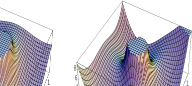
Figure 1: The potential $V_{C}=\overline{v_{C}(\Phi)}v_{C}(\Phi)$ for the center-vortex condensate $\Phi$. Notice the regions of negative tangential curvature in between the minima.

The ridges of negative tangential curvature are classically forbidden: The field $\Phi$ tunnels through these ridges, and a phase change, which is determined by an element of the center $Z_{2}$ (SU(2)) or $Z_{3}$ (SU(3)), occurs locally in space. This is the afore-mentioned generation of one unit of center flux.

To decide about the absence of fluctuations in each of the minima of the potential $V_{C}$ the following consideration applies. First of all, one compares the curvature at the minima with the square of the coarse-graining scale $|\Phi_{\tiny\mbox{min}}|=\Lambda_{C}$. Setting $\Phi=|\Phi|\,\exp(i\frac{\theta}{|\Phi|})$ one has

$$\left.\frac{\partial^{2}_{\theta}V_{C}(\Phi)}{|\Phi|^{2}}\right|_{\Phi_{\tiny\mbox{min}}}=\left.\frac{\partial^{2}_{|\Phi|}V_{C}(\Phi)}{|\Phi|^{2}}\right|_{\Phi_{\tiny\mbox{min}}}=\left\{\begin{array}[]{c}8\,\ \ \ \ \ (\mbox{SU(2)})\\ 18\,\ \ \ \ \ (\mbox{SU(3)})\end{array}\right.\,.$$ (16)

Thus a potential fluctuation $\delta\Phi$ would be harder than the maximal resolution $|\Phi_{\tiny\mbox{min}}|$ corresponding to the effective action that arises after spatial coarse-graining, and therefore $\delta\Phi$ is already contained in the classical configuration $\Phi_{\tiny\mbox{min}}$: $\delta\Phi$ does not exist in the effective theory. Second, we need to investigate whether tunneling events take place that lift the degeneracy of the minima. According to the WKB-method the probability of a tunneling event to another minimum is given by $\exp(-S_{\tiny\mbox{tunn}})$ where the subscript ‘tunn’ refers to a classical, euclidean trajectory connecting the minima. This trajectory must be BPS saturated since the tunneling event itself is spontaneous: no energy is needed (and apriori present) for it to occur. In [18] BPS saturated trajectories subject to the potentials in Eqs. (13) and (15) have been investigated. The only solution to the BPS equation, subject to the initial condition $\Phi=\Phi_{\tiny\mbox{min}}$, is $\Phi\equiv\Phi_{\tiny\mbox{min}}$ for any finite amount of euclidean time $\tau$. Since there are no fluctuations $\delta\Phi$ available that could possibly alter the initial condition $\Phi=\Phi_{\tiny\mbox{min}}$ we conclude that tunneling processes are entirely absent. (Viewed alternatively, one would have to wait infinitely long for a tunneling process to occur.) We conclude that once the field $\Phi$ has relaxed to either one of the minima of the potential $V_{C}$ no quantum fluctuations are around that could possibly shift the vanishing ground-state pressure and energy density of the theory. Needless to say, this result is relevant for an understanding of the smallness of today’s value of the cosmological constant on particle-physics scales.

The density of massive spin-1/2 states, that is generated in the process of relaxation, is over-exponentially increasing. Namely, the multiplicity of massive fermion states, associated with center-vortex loops possessing $n$ selfintersections, is given by twice the number $L_{n}$ of bubble diagrams with $n$ vertices in a scalar $\lambda\phi^{4}$ theory. (In the absence of propagating gauge modes, possibly provided by another Yang-Mills theory, we disregard charge multiplicities.) In [19] the minimal number of such diagrams $L_{n,min}$ was estimated to be

$$L_{n,min}=n!3^{-n}\,.$$ (17)

The mass spectrum is equidistant: The mass $m_{n}$ of a state with $n$ selfintersections of the center-vortex loop is $m_{n}\sim n\,\Lambda_{C}$. If we only ask for an estimate of the density of static fermion states $\rho_{n,0}=\tilde{\rho}(E=n\Lambda_{C})$ of energy $E$ then, by appealing to Eq. (17) and Stirling’s formula, we obtain [4]

$$\rho_{n,0} > \frac{\sqrt{8\pi}}{3\Lambda_{C}}\,\exp[n\log n]\Big{(}\log n+1\Big{)}\,\ \ \ \ \ \mbox{or}$$

$$\tilde{\rho}(E) > \frac{\sqrt{8\pi}}{3\Lambda_{C}}\exp[\frac{E}{\Lambda_{C}}\log\frac{E}{\Lambda_{C}}]\Big{(}\log\frac{E}{\Lambda_{C}}+1\Big{)}\,.$$ (18)

The partition function $Z_{\Phi}$ for the system of static fermions thus is estimated as

$$Z_{\Phi} > \int_{E^{*}}^{\infty}dE\,\tilde{\rho}(E)\,n_{F}(\beta E)$$ (19)

$$> \frac{\sqrt{8\pi}}{3\Lambda_{C}}\,\int_{E^{*}}^{\infty}dE\,\exp\left[\frac{E}{\Lambda_{C}}\right]\,\exp[-\beta E]\,,$$

where $E^{*}\gg\Lambda_{C}$ is the energy where we start to trust our approximations. Thus $Z_{\Phi}$ diverges at some temperature $T_{H}<\Lambda_{C}$. Due to the logarithmic factor in the exponent arising in estimate Eq. (4) for $\tilde{\rho}(E)$ we would naively conclude that $T_{H}=0$. This, however, is an artefact of our assumption that all states with $n$ selfintersections are absolutely stable. Due to the existence of contact interactions between vortex lines and intersection points this assumption is the less reliable the higher the total energy of a given fluctuation. (A fluctuation of large energy has a higher density of intersection points and vortex lines and thus a larger likelihood for the occurrence of contact interactions which mediate the decay or the recombination of a given state with $n$ selfintersections.) At the temperature $T_{H}$ the entropy wins over the Boltzmann suppression in energy, and the partition function diverges. To reach the point $T_{H}$ one would, in a spatially homogeneous way, need to invest an infinite amount of energy into the system which is impossible. By an (externally induced) violation of spatial homogeneity and thus by a sacrifice of thermal equilibrium the system may, however, condense densly packed (massless) vortex intersection points into a new ground state. The latter’s excitations exhibit a power-like density of states and thus are described by a finite partition function. This is the celebrated Hagedorn transition approached from below [20].

5 Thermodynamical quantities throughout the deconfining and preconfining phase

Here we indicate the temperature dependence of the pressure $P$ (Fig. 2), the energy density $\rho$ (Fig. 3), and the entropy density $S$ (Fig. 4).

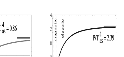
Figure 2: $\frac{P}{T^{4}}$ as a function of temperature for SU(2) (left panel) and SU(3) (right panel). The horizontal lines indicate the respective asymptotic values, the dashed vertical lines are the phase boundaries.

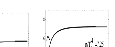
Figure 3: $\frac{\rho}{T^{4}}$ as a function of temperature for SU(2) (left panel) and SU(3) (right panel). The horizontal lines indicate the respective asymptotic values, the dashed vertical lines are the phase boundaries.

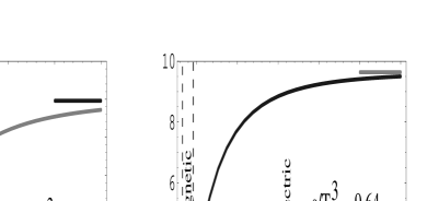
Figure 4: $\frac{S}{T^{3}}$ as a function of temperature for SU(2) (left panel) and SU(3) (right panel). The horizontal lines signal the respective asymptotic values.

Notice the negativity of the pressure at low temperatures. Notice also that all thermodynamical quantities reach their Stefan-Boltzmann limits very rapidly. At $T_{c,M}$ the pressure is discontinuous: It is positive and very large shortly below $T_{c,M}$ (Hagedorn transition). The entropy density vanishes at $T_{c,M}$: At this point the SU(2) or the SU(3) Yang-Mills theory only generates a cosmological constant.

6 Some implications: SU(2)${}_{\tiny\mbox{CMB}}\stackrel{{\scriptstyle\tiny\mbox{today}}}{{=}}$U(1)_Y

We only discuss implications arising from a modification of the gauge group describing photon propagation. Other implications are briefly discussed in [4] and [22].

In [4, 6, 21, 22] we have discussed why the U(1) gauge symmetry of electromagnetism is likely to have an SU(2) instead of an U(1)_Y progenitor. To comply with the observational fact, that the photon is massless and unscreened [23] within the present cosmological epoch, $T_{c,E}$ must coincide with the temperature $T_{\tiny\mbox{CMB}}\sim 2.7\,$K of the cosmic microwave background (CMB). Hence the name SU(2)${}_{\tiny\mbox{CMB}}$.

There emerges a number of unexpected results when subjecting the dynamics of SU(2)${}_{\tiny\mbox{CMB}}$ to a thermodynamical treatment.

First, one deduces that the present ground-state energy density of SU(2)${}_{\tiny\mbox{CMB}}$ is less than 0.4% of the measured value of today’s density in dark energy [22]. Thus there must be an additional mechanism providing for the latter. A serious possibility is that a Planck-scale axion field, coupling to the topological defects of SU(2)${}_{\tiny\mbox{CMB}}$ and thereby acquiring a tiny mass ($m_{\tiny\mbox{axion}}\sim 10^{-36}\,$eV), is caught at the slope of its potential by cosmological friction. This axion field owes its existence to the chiral anomaly [24] taking place due to integrated-out chiral fermions as the temperature of the Universe fell below the Planck mass $M_{P}\sim 1.2\times 10^{19}\,$GeV. These fermions may have emerged because an SU(2) or an SU(3) gauge theory of Yang-Mills scale $\Lambda\sim M_{P}$ went confining. A (to-be-investigated) possibility is that all SU(2) or SU(3) gauge symmetries together with their Yang-Mills scales, describing the matter content of our (four-dimensional) Universe, were set by a dynamical symmetry breakdown: SU($\infty)\to$ gravity + matter. The Planck mass would then be associated with the Yang-Mills scale of SU($\infty$). The Planck-scale axion would trigger CP-violation in particle creation whenever an SU(2) or an SU(3) factor becomes nervous, that is, close to a Hagedorn transition (matter asymmetry [25]).

Second, one derives that due to the present cosmological expansion, mainly driven by the axion field, the photon remains massless only for a period $\Delta t_{m_{\gamma}=0}$ of at most 2 billion years [22]: After the time $\Delta t_{m_{\gamma}=0}$ has elapsed the photon acquires a Meissner mass (transition from deconfining to preconfining phase), and the ground-state of the Universe becomes superconducting. To obtain a tighter upper estimate for $\Delta t_{m_{\gamma}=0}$ one would have to relate the strength of intergalactic magnetic fields to the exact point in the phase diagram of SU(2)${}_{\tiny\mbox{CMB}}$ corresponding to the present supercooled state of the Universe.

Third, if photon propagation is described by SU(2)${}_{\tiny\mbox{CMB}}$ rather than U(1)_Y then a visible modification of black-body spectra is predicted [6, 26] for temperatures not much above $T_{\tiny\mbox{CMB}}$, see Fig, 5.

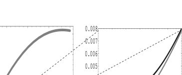
Figure 5: Dimensionless black-body spectral power $\frac{I_{\tiny\mbox{SU(2)}}}{T^{3}}$ as a function of the dimensionless frequency $Y\equiv\frac{\omega}{T}$. The black curve in the magnified region depicts the modification of the spectrum as compared to $\frac{I_{\tiny\mbox{U(1)}}}{T^{3}}$ (grey curve) for $T=10\,$K.

The spectral gap at low frequencies may explain why cold (brightness temperature $T_{B}=5\cdots 10\,$K) and dilute (particle distance $\sim 1\,$cm) clouds in between the spiral arms of the outer galaxy are composed of atomic instead of molecular hydrogen and why such a situation is stable [27, 28, 29]. If SU(2)${}_{\tiny\mbox{CMB}}$ is experimentally supported by the observation of the spectral gap in the black-body spectra at low temperatures then a contradition to the Standard Model’s scenario for Big-Bang nucleosythesis arises. Namely, additional six relativistic degrees of freedom are present at the freeze-out temperature $T_{\tiny\mbox{freeze-out}}\sim 1\,$MeV for proton-to-neutron conversion implying a larger value of the Hubble parameter in comparison to the Standard Model. The proton-to-neutron ratio at freeze-out, which determines $T_{\tiny\mbox{freeze-out}}$, is rather tightly constrained by the relative abundance $Y_{p}$ of primordial ⁴He [30]. One possibility to cure the mismatch in relativistic degrees of freedom would be to prescribe a larger value of the Fermi coupling $G_{F}$ at $T_{\tiny\mbox{freeze-out}}$. If the weak interactions and the emergence of the electron and its neutrino are described by an SU(2) gauge theory of Yang-Mills scale $\Lambda\sim 0.5\,$MeV then an enhancement of $G_{F}$ is, indeed, expected. Notice, however, that at $T_{\tiny\mbox{freeze-out}}\sim 1\,$MeV this theory is close to its Hagedorn transition; thus meaning that the synthesis of light elements would have taken place in a nonthermal environment.

References

-
[1]
F. J. Dyson, Phys. Rev. 85, 631 (1952).
C. A. Hurst, Proc. Camb. Phil. Soc. 48, 625 (1952).
W. Thirring, Helv. Phys. Acta 26, 33 (1953).
A. Peterman, Helv. Phys. Acta 26, 291 (1953).
L. S. Brown and L. G. Yaffe, Phys. Rev. D 45, 398 (1992).
V. I. Zakharov, Nucl. Phys. B 385, 452 (1992).
A. H. Mueller, in QCD: 20 Years later. Aachen, Germany, 1992, ed. P. M. Zerwas and H. A. Kastrup (World Scientific, Singapore, 1993). - [2] A. D. Linde, Phys. Lett. B 96, 289 (1980).
- [3] A. M. Polyakov, Phys. Lett. B 59, 82 (1975).
- [4] R. Hofmann, Int. J. Mod. Phys. A 20, 4123 (2005).
- [5] U. Herbst, R. Hofmann, and J. Rohrer, Acta Phys. Pol. B 36, 881 (2005).
- [6] M. Schwarz, R. Hofmann, and F. Giacosa, hep-th/0603078.
- [7] B. J. Harrington and H. K. Shepard, Phys. Rev. D 17, 105007 (1978).
- [8] U. Herbst and R. Hofmann, hep-th/0411214.
- [9] G. ’t Hooft, Nucl. Phys. B 33 (1971) 173. G. ’t Hooft and M. J. G. Veltman, Nucl. Phys. B 44, 189 (1972). G. ’t Hooft, Int. J. Mod. Phys. A 20 (2005) 1336 [arXiv:hep-th/0405032].
- [10] N. P. Landsman and C. G. van Weert, Phys. Rept. 145, 141 (1987).
- [11] W. Nahm, Lect. Notes in Physics. 201, eds. G. Denaro, e.a. (1984) p. 189.
- [12] T. C. Kraan and P. van Baal, Nucl. Phys. B 533, 627 (1998).
- [13] T. C. Kraan and P. van Baal, Phys. Lett. B 435, 389 (1998).
- [14] K.-M. Lee and C.-H. Lu, Phys. Rev. D 58, 025011 (1998).
- [15] D. Diakonov, N. Gromov, V. Petrov, and S. Slizovskiy, Phys. Rev. D 70, 036003 (2004) [hep-th/0404042].
- [16] L. Del Debbio et al., proc. NATO Adv. Res. Workshop on Theor. Phys., Zakopane (1997) [hep-lat/9708023].
- [17] H. Reinhardt, Nucl. Phys. B 628, 133 (2002).
- [18] R. Hofmann, Phys. Rev. D 62, 065012 (2000).
- [19] C. M. Bender and T. T. Wu, Phys. Rev. 184, 1231 (1969).
- [20] R. Hagedorn, Nuovo Cim. Suppl. 3, 147 (1965).
- [21] R. Hofmann, PoS JHW2005, 021 (2006) [hep-ph/0508176].
- [22] F. Giacosa and R. Hofmann, hep-th/0512184.
- [23] E. R. Williams, J. E. Faller, and H. A. Hill, Phys. Rev. Lett. 26, 721 (1971).
-
[24]
S. L. Adler, Phys. Rev. 177, 2426 (1969).
S. L. Adler and W. A. Bardeen, Phys. Rev. 182, 1517 (1969).
J. S. Bell and R. Jackiw, Nuovo Cim. A 60, 47 (1969).
K. Fujikawa, Phys. Rev. Lett. 42, 1195 (1979). - [25] A. D. Sakharov, Pisma Zh. Eksp. Teor. Fiz. 5, 32 (1967); JETP Lett. 5, 24 (1967); Sov. Phys. Usp. 34, 392 (1991); Usp. Fiz. Nauk 161, 61 (1991).
- [26] M. Schwarz, R. Hofmann, and F. Giacosa, hep-ph/0603174.
- [27] L. B. G. Knee and C. M. Brunt, Nature 412, 308 (2001).
- [28] J. M. Dickey, Nature 412, 282 (2001).
-
[29]
D. W. Kavars et al., Astrophys. J. 626, 887 (2005).
D. W. Kavars and J. M. Dickey et al., Astrophys. J. 598, 1048 (2003).
N. M. McClure-Griffiths et al., astro-ph/0503134. - [30] B. D. Fields and S. Darkar in S. Eidelman et al.: Particle Data Group: Reviews, Tables, and Plots. Phys. Lett. B 592, 202 (2004).