FTPI-MINN-06/11, UMN-TH-2439/06
ITEP-TH-10/06
April 27, 2006
Bulk–Brane Duality in Field Theory
M. Shifmana and A. Yunga,b,c
aWilliam I. Fine Theoretical Physics Institute,
University of Minnesota,
Minneapolis, MN 55455, USA
bPetersburg Nuclear Physics Institute, Gatchina, St. Petersburg
188300, Russia
cInstitute of Theoretical and Experimental Physics, Moscow
117259, Russia
Abstract
We consider (3+1)-dimensional supersymmetric QED with two flavors of fundamental hypermultiplets. This theory supports 1/2-BPS domain walls and flux tubes (strings), as well as their 1/4-BPS junctions. The effective (2+1)-dimensional theory on the domain wall is known to be a U(1) gauge theory. Previously, the wall–string junctions were shown to play the role of massive charges in this theory. However, the field theory of the junctions on the wall (for semi–infinite strings) appears to be inconsistent due to infrared problems. All these problems can be eliminated by compactifying one spatial dimension orthogonal to the wall and considering a wall–antiwall system () on a cylinder. We argue that for certain values of parameters this set-up provides an example of a controllable analog of bulk–brane duality in field theory. Dynamics of the 4D bulk are mapped onto 3D boundary theory: 3D SQED with two matter superfields and a weak–strong coupling constant relation in 4D and 3D, respectively. The cylinder radius is seen as a “real mass” in 3D SQED. We work out (at weak coupling) the quantum version of the world-volume theory on the walls. Integrating out massive matter (strings in the bulk theory) one generates a Chern–Simons term on the wall world volume and an interaction between the wall and antiwall that scales as a power of distance. Vector and scalar (classically) massless excitations on the walls develop a mass gap at the quantum level; the long-range interactions disappear. The above duality implies that the wall and its antiwall partner (at strong coupling in the bulk theory) are stabilized at the opposite sides of the cylinder.
1 Introduction
Duality is one of the most fascinating ideas in theoretical physics. Basically, duality means that one and the same dynamical system can be described using two different theories. Moreover, when one description is in the weak coupling regime, the second is at strong coupling and vice versa. This makes duality extremely hard to prove. Exceptions are theories where one can find exact solutions and continue them from weak to strong coupling. The most well-known example is electromagnetic duality in gauge theories [1, 2]. In other cases duality is conjectured, e.g. AdS/CFT correspondence [3, 4, 5], and then indirectly verified. On the other hand, once duality is confirmed, it becomes a powerful tool to study theories at strong coupling using their weakly coupled duals.
AdS/CFT correspondence provides an example of duality between theories with different dimensions. On the one side is a string theory in the bulk which, in a certain limit, reduces to a classical supergravity model. A gauge theory on the four-dimensional boundary of the five-dimensional bulk is on the other side of AdS/CFT.
In this paper we present a purely field-theoretic example of such “holographic” duality. We consider (3+1)-dimensional gauge theory with domain walls and flux tubes (strings) as our bulk model. One of the spatial dimensions is compactified, so that in fact our four-dimensional bulk is . We show that a system of two parallel walls and strings stretched between these walls has a dual description in terms of (2+1)-dimensional U(1) gauge theory on the world volume of domain walls. In three dimensions the dual model has (four supercharges). Moreover, the weak coupling regime in the bulk theory corresponds to strong coupling in the world-volume theory and vice versa. As it often happens, we cannot rigorously prove duality in this case. However, we are able to provide indirect evidence and to explicitly determine a condition which ensures duality.
Our bulk theory is supersymmetric QED with 2 flavors of charged matter hypermultiplets and the Fayet-Iliopoulos term [6]. In this theory one can construct both, the 1/2 BPS-saturated walls and strings. Moreover, the 1/4 BPS-saturated wall-string junctions exist too [7]. In the domain wall world-volume theory these junctions are seen as “electric charges” of dual QED. However, construction of the world-volume theory, with the electric charges (a.k.a. junctions) included, was hampered by the fact that the string attached to the given junction was assumed to be semi-infinite [7]. Thus, it could not be mapped to any local theory on the domain wall. A way out was suggested by Tong in the inspiring paper [8]. He suggested to consider two parallel domain walls at finite distance from each other, connected by a finite-length string. As will be discussed in the bulk of the paper, the concrete set-up presented in [8] has no mass shell, due to long-range (scalar-field-mediated) interactions which result in an infinite bending of the walls at infinity. Building on Tong’s proposal and our previous results we develop a consistent construction implementing the bulk–brane duality in field theory. To the best of our knowledge, this is the first example of this type. We hasten to warn the reader that the above duality must be understood in a limited sense. Usually the phrases “brane-bulk duality” or “holographic description” apply to AdS/CFT where the the boundary theory sees everything that happens in the bulk. This certainly is not true of the theory on the domain walls we discuss. For example, our 3D theory has no way of knowing about such degrees of freedom in the bulk as particles collisions far from the branes. In this sense, we deal with a “blurred holography.”
We show that infrared problems can be eliminated by compactifying one spatial dimension orthogonal to the wall and considering a wall-antiwall system on a cylinder. If the radius of the cylinder is much larger than the wall thickness, classically, the relative distance between the walls is a modulus. The corresponding excitations are gapless. Supersymmetry then predicts that other states from the same supermultiplet, namely, the photon and its fermion partners, are massless too. If we place classical static sources of the dual electromagnetic field and the scalar field on the wall, the induced interactions do not fall off at infinity. A generic string–brane configuration has infinite energy. A finite energy is obtained on configurations of a very special type — with equal number of string connections on both sides of the cylinder.
We work out the quantum version of the 3D theory on the walls and show that taking account of quantum effects drastically changes the situation. The massive matter (a.k.a. strings in the bulk theory) generates a Chern–Simons term on the wall world volume and produces a quadratically rising interaction potential between the wall and antiwall, with the minimum of the potential energy corresponding to the wall and antiwall located at the opposite sides of the cylinder. The moduli of the classical theory are lifted. There are no long-range forces on the wall.
The paper is organized as follows. In Sect. 2 we introduce our bulk theory and briefly review BPS domain wall and string solutions in this theory. In Sect. 3 we review the 1/4-BPS solution for the string-wall junction and represent this junction as a classical charge in the (2+1)-dimensional low-energy effective theory on the wall. In Sect. 4 we consider wall-antiwall system on a cylinder and suggest a quantum version of the theory on the walls. We also discuss bulk–brane duality. In Sect. 5 we discuss physics of the world-volume theory and show that both the Chern–Simons term and quadratic wall-antiwall interaction potential are generated at the quantum level. Section 6 contains our conclusions while Appendix deals with formulation of (2+1)-dimensional QED and parity anomaly.
2 Domain walls and strings
The bulk theory which we will work with is SQED with 2 flavors. It supports both, the BPS-saturated domain walls and, if the Fayet–Iliopoulos term is added, the BPS-saturated ANO strings. The bosonic part of the action of the bulk theory is 111Here we use Euclidean notation; we switch to Minkowskian notation in Sect. 5 and Appendix.
| (2.1) |
where
| (2.2) |
Here is the coefficient in front of the Fayet-Iliopoulos term, is the U(1) gauge coupling, the index is the flavor index; and the mass parameters are assumed to be real. In addition we will assume
| (2.3) |
Simultaneously, . There are two vacua in this theory: in the first vacuum
| (2.4) |
and in the second one
| (2.5) |
The vacuum expectation value (VEV) of the field vanishes in both vacua. Hereafter we will stick to the ansatz .
A BPS domain wall interpolating between the two vacua of our bulk theory was explicitly constructed in Ref. [7]. Assuming that all fields depend only on the coordinate , it is possible to write the energy in the Bogomol’nyi form [9],
| (2.6) | |||||
Requiring the first two terms above to vanish gives us the BPS equations for the wall. Assuming that we choose the upper sign in (2.6). The tension is given by the total derivative term (the last one in Eq. (2.6)) which can be identified as the central charge of the supersymmetry algebra,
| (2.7) |
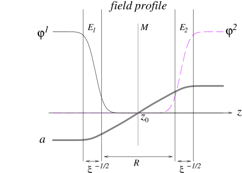
The wall solution has a three-layer structure (see Fig. 1): in the two outer layers (which have width )) the squark fields drop to zero exponentially; in the inner layer the field interpolates between its two vacuum values. The thickness of this inner layer is given by
| (2.8) |
This wall is an BPS solution of the Bogomol’nyi equations. In other words, the soliton breaks four of eight supersymmetry generators of the bulk theory. In fact, as was shown in [7], the four supercharges selected by the conditions
| (2.9) |
act trivially on the wall solution. Here and are eight supertransformation parameters.
The moduli space is described by two bosonic coordinates: one of these coordinates is associated with the wall translation; the other one is a U(1) compact parameter . Its origin is as follows [7]. The bulk theory at has U(1)U(1) flavor symmetry corresponding to two independent rotations of two quark flavors. In both vacua only one quark develops a VEV. Therefore, in both vacua only one of these two U(1)’s is broken. The corresponding phase is eaten by the Higgs mechanism. However, on the wall both quarks have nonvanishing values, breaking both U(1) groups. Only one of corresponding two phases is eaten by the Higgs mechanism. The other one becomes a Goldstone mode living on the wall.
It is possible to promote these moduli to fields depending on the wall coordinates (). Then, deriving a world-volume theory for the moduli fields on the wall is straightforward. The U(1) phase discussed above can be dualized [10] to a U(1) gauge field in (2+1) dimensions. Thus, the world-volume theory is a U(1) gauge theory. The domain wall under consideration can be interpreted as a -brane prototype in field theory [11, 12, 13, 7]. The bosonic part of the world-volume action is
| (2.10) |
where describes the translational mode while
is the coupling constant of the effective U(1) theory on the wall related to the parameters of the bulk theory as
| (2.11) |
The fermion content of the world-volume theory is given by two three-dimensional Majorana spinors, as is required by in three dimensions. The full world-volume theory is a U(1) gauge theory in dimensions, with four supercharges. The Lagrangian and the corresponding superalgebra can be obtained by reducing four-dimensional SQED (with no matter) to three dimensions (see Appendix).
The field in (2.10) is the superpartner of the gauge field . To make it more transparent we make a rescaling, introducing a new field
| (2.12) |
In terms of the action (2.10) takes the form
| (2.13) |
The gauge coupling constant has dimension of mass in three dimensions. A characteristic scale of massive excitations on the world volume theory is of the order of the inverse thickness of the wall , see (2.8). Thus the dimensionless parameter that characterizes the coupling strength in the world-volume theory is ,
| (2.14) |
We interpret this as a feature of the bulk–wall duality: the weak coupling regime in the bulk theory corresponds to strong coupling on the wall and vice versa [7]. Of course, finding explicit domain wall solutions and deriving the effective theory on the wall assumes weak coupling regime in the bulk, . In this limit the world-volume theory is in the strong coupling regime and is not very useful.
Our theory (2.1) is Abelian and as such does not have monopoles. However, we could have compactified U(1), starting from the non-Abelian theory with the gauge group SU(2), broken down to U(1) by condensation of the adjoint scalar field (whose third component is , see (2.4) and (2.5)). This non-Abelian theory would have the ’t Hooft-Polyakov monopoles [14]. In the low-energy limit (2.1) these monopoles become heavy external magnetic charges, with mass of the order of . Once electrically charged fields condense in both vacua (2.4) and (2.5), these monopoles are in the confining phase in both vacua.
In fact, in each of the two vacua of the bulk theory the magnetic charges are confined by the Abrikosov–Nielsen–Olesen (ANO) strings [15]. In the vacuum in which we can use the ansatz and write the following BPS equations:
| (2.15) |
where
Analogous equations can be written for the flux tube in the other vacuum, . These objects are half-critical, much in the same way as the domain walls above.
The magnetic flux of the minimal-winding flux tube is , while its tension is given by the central charge [16],
| (2.16) |
The thickness of the tube is of the order of
| (2.17) |
3 Wall–string junctions
Let us consider a flux tube ending on a domain wall. The flux tube is semi-infinite and aligned perpendicular to the wall. This configuration was studied in gauge theories in Refs. [7, 17, 18, 19] (for a review see [20, 21]) and, earlier, in four-dimensional sigma models [13].
Consider a vortex oriented in the direction ending on a wall oriented in the plane; let the string extend at and let the magnetic flux be oriented in the negative direction. The BPS first-order equations can be written for the composite soliton [7],
| (3.1) |
These equations generalize both the -BPS wall and string equations and were used to determine the general -BPS solution for the string-wall junction, (i.e. a flux tube ending on the wall).
These equations were derived in [7] as follows. The first-order equations for 1/2-BPS string can be obtained by imposing the requirement that four supercharges of the bulk theory selected by the conditions [22]
| (3.2) |
act trivially on the string solution. Then, imposing both wall and string conditions (2.9) and (3.2) to select two supercharges which act trivially on the string-wall junction, we obtain the first-order equations (3.1).
The solution for the string-wall junction at large distance from the string end-point has the form of a wall solution with the collective coordinates and the U(1) phase depending on the world-volume coordinates and . Namely [7], the wall is logarithmically bent due to the fact that the vortex pulls it,
| (3.3) |
Moreover, the magnetic flux from the string penetrates into the wall and, therefore, the string end-point is seen as an electric charge in the world-volume theory, dual QED.222Here the word “dual” is used in the sense of electromagnetic (nonholographic) duality, with the phase dualized à la Polyakov [10] to be traded for the 3D gauge field . The electric field at large distances from the string-wall junction is given by
| (3.4) |
where .
In the world-volume theory per se, the fields (3.3) and (3.4) can be considered as produced by classical point-like charges which interact in a standard way with the electromagnetic field and the scalar field ,
| (3.5) | |||||
where the classical electromagnetic current and the charge density of a static charge is given by
| (3.6) |
for a unit charge located at . To derive (3.5) we used (3.3) and (3.4), as well as the relation (2.12). Thus, the string is seen in the world-volume theory on the wall as a unit static charge.
It is easy to calculate the energy of this static charge. There are two distinct contributions to this energy [23]. The first contribution is due to the gauge field,
| (3.7) | |||||
The integral is logarithmically divergent both in the ultraviolet and infrared. It is clear that the UV divergence is cut off at the transverse size of the string (2.17) and presents no problem. However, the infrared divergence is much more serious. We introduced a large size to regularize it in (3.7).
The second contribution, due to the field, is proportional to too,
| (3.8) | |||||
Both contributions are logarithmically divergent in the infrared. Their occurrence is an obvious feature of charged objects coupled to massless fields in dimensions due to the fact that the fields and do not die off at infinity which means infinite energy.
The above two contributions are equal (with the logarithmic accuracy), even though their physical interpretation is different. The total energy of the string junction is
| (3.9) |
We see that in our attempt to include strings as point-like charges in the world-volume theory (3.5) we encounter problems already at the classical level. The energy of a single charge is IR divergent. (This is on top of the fact that semi-infinite strings in the bulk have masses proportional to their length; once the length is infinite so are their masses. For the time being we will disregard the latter aspect, to be addressed below.)
It is clear that the infrared problems will become even more severe in quantum theory. One might suggest to overcome this problem by adding antistrings in our picture. The antistring carries an opposite magnetic flux to that of the string; therefore, it produces the following (dual) electric field on the wall:
| (3.10) |
while the bending of the wall due to the string stretched at is still given by Eq. (3.3). The fields (3.3), (3.4) of the string and (3.3), (3.10) of the antistring can be described by the world-volume action (3.5) where the currents and are given by
| (3.11) |
Here and are electric and scalar charges associated with the string end with respect to the electromagnetic field and the scalar field , respectively,
The string with incoming flux has the charges while the string with outgoing flux (the antistring) the charges .
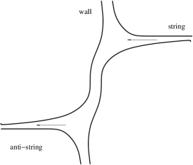
Now we can consider a configuration with equal number of strings and antistrings so that at large distances from their end-points the electric field has a power fall-off and produces no IR divergence, see Fig. 2. This solves only a half of the problem, however. The electric fields produced by the string and antistring cancel each other at large . At the same time, the bending of the wall is doubled, as it is clear from Eq. (3.11) and Fig. 2. Thus, the wall bending energy is still IR divergent.333This aspect was omitted in [8]. For further discussion see Sect. 4.

A way out was suggested in [23]. For the infrared divergences to cancel we should consider strings coming to the wall from the right and from the left. Clearly, the bending of the wall produced by the string coming from the left is given by
| (3.12) |
It has the opposite sign as compared to the bending of the string coming from the right. Thus, we have the following set of the electric (scalar) charges associated with the string end-points:
| (3.13) |
while their scalar charges are
| (3.14) |
Clearly, the bending of the wall produced by two string attached from different sides of the wall tends to zero at large from the string end-points and produces no IR divergence. In fact, it was shown in [23] that the configuration depicted in Fig. 3 is a non-interacting 1/4-BPS configuration. All logarithmic contributions are canceled; the junction energy in this geometry is given by a finite negative contribution
| (3.15) |
In Sect. 4 we will consider a wall configuration in which the attached strings can appear from both sides of the wall. Then we will suggest a quantum version of the theory on the wall.
4 Quantizing strings on the wall
In this section we will work out a quantum version of the world-volume theory (3.5) with charged matter fields which, on the world volume, represent strings of the bulk theory. First we proceed in the spirit of Ref. [8], and then deviate in a bid for a theory free of IR divergences. A novel element is introduction of two types of charged matter, to represent both, strings attached from the left and from the right of the wall.
The mass of the string is equal to its tension (2.16) times its length. If we have a single wall, all strings attached to it have infinite length; therefore, they are infinitely heavy. In the world-volume theory on the wall (3.5) they are seen as classical infinitely heavy point-like charges. In order to quantize these charges one has to make their masses finite. To this end one needs at least two domain walls [8].
Let us describe our set-up in some detail. First, we compactify the direction in our bulk theory (2.1), on a circle of length . Then we consider a pair “wall plus antiwall” oriented in the plane, separated by a distance in the perpendicular direction, see Fig. 4. The wall and antiwall experience attractive forces. Strictly speaking, this is not a BPS configuration — supersymmetry in the world-volume theory is broken. However, the wall-antiwall interaction due to overlap of their profile functions is exponentially suppressed at large separations,
| (4.1) |
where is the wall size (see Eq. (2.8)). In what follows we neglect exponentially suppressed effects. If so, we neglect effects which break supersymmetry in our (2+1)-dimensional world-volume theory. Thus, it continues to have four conserved supercharges (supersymmetry in (2+1) dimensions) as was the case for the isolated single wall.

Although our set-up contains the wall-antiwall pair, in fact, the world-volume theory we will derive is that on the single wall (or single antiwall); the presence of the second component is irrelevant. This is due to our specific choice of relevant parameters. Neither walls nor strings can be excited in the range of parameters we work. This means that whatever happens on the surface the wall, unambiguously fixes what happens on the surface of the antiwall and vice versa. In this sense, our holography is peculiar and is not similar to the situation in string theory. Our holography relates phenomena seen on one wall (or, which is the same, on one antiwall) to the bulk physics of “minimal” (non-excited, “straight”) strings stretched between the wall and antiwall. This is why in fact our world-volume theory has four supercharges, and the particle supermultiplets on the world volume are short.
One can try to formalize the above intuitive arguments as follows. The wall preserves four supercharges determined by the conditions (2.9). The antiwall preserves four other supercharges determined by the same conditions with the opposite sign,
| (4.2) |
Let us consider a new z-dependent SUSY transformation defined on two patches. The wall patch is at
while the antiwall patch is at
where we denote the wall position by and that of the antiwall by , assuming
to be large.
Now, define four new supercharges as selected by the condition (2.9) on the wall patch and by the condition (4.2) on the antiwall patch. This new SUSY transformation acts almost trivially on the wall-antiwall solution (up to exponentially small terms coming from the antiwall tail in the wall patch, and the wall tail in the antiwall patch). As soon as the space is almost empty at two points and , there are no problems of gluing these two patches together (there are some -function contributions in the SUSY algebra, to be taken care of, but these give (almost) zero acting on the wall-antiwall system). These are exactly the four SUSY charges acting in our world-volume theory.
Let us consider this theory in more detail. The kinetic terms for the fields and in the world-volume theory are obvious, (see (2.10))
| (4.3) |
where we use (2.12) to define the fields . The sum of these fields,
with the corresponding superpartners, decouples from other fields forming a free field theory describing dynamics of the center of mass of our construction. This is a trivial part which will not concern us here.
An interesting part is associated with the field
| (4.4) |
The factor ensures that has a canonically normalized kinetic term. By definition, it is related to the relative wall-antiwall separation, namely,
| (4.5) |
Needless to say, has all necessary superpartners. In the bosonic sector we introduce the gauge field
| (4.6) |
with the canonically normalized kinetic term.
Now, let us include the classical string solutions attached to the wall and antiwall. The BPS conditions for the string are given in Eq. (3.2). The string-wall-antiwall junction is a 1/4-BPS object. Two supercharges acting trivially on this junction are defined by (2.9) and (3.2) in the wall patch, and by (4.2) and (3.2) in the antiwall patch. Thus, the string is described by a short chiral multiplet in the world-volume theory.
In quantum theory the strings stretched between the wall and antiwall, on both sides, will be represented by two chiral superfields, and , respectively. We will denote the corresponding bosonic components by and .
In terms of these fields the quantum version of the theory (3.5) is completely determined by the charge assignment (3.13), (3.14) and supersymmetry. The charged matter fields have the opposite electric charges and distinct mass terms, see below. A mass term for one of them is introduced by virtue of a “real mass,” as is explained in Appendix. It is necessary due to the fact that there are two interwall distances, and . The real mass breaks parity. The bosonic part of the action has the form
| (4.7) | |||||
We will present additional comments on the derivation of this expression in Sect. 5. According to our discussion in Sect. 3, the fields and have charges +1 and with respect to the gauge fields and , respectively. Hence,
| (4.8) |
The electric charges of strings with respect to the field are . The last term in (4.7) is the -term dictated by supersymmetry. So far, is a free parameter whose relation to will be determined shortly. Moreover, . The theory (4.7) with the pair of chiral multiplets and is free from IR divergences and global anomalies [24, 25]. On the classical level it is clear from our discussion in the previous section. In Ref. [8] a version of the world volume theory (4.7) with only one supermultiplet was considered.
Now we make a crucial test of our theory (4.7) calculating the masses of charged matter multiplets and . From (4.7) we see that the mass of is given by
| (4.9) |
Substituting here the relation (4.5) we get
| (4.10) |
The mass of the charged matter field is equal to the mass of the string of the bulk theory stretched between the wall and antiwall at separation , see (2.16). Of course, this was expected. Note that this is a nontrivial check of the consistency of our world-volume theory with the bulk theory. Indeed, the charges of strings end-points (3.13) and (3.14) are fixed by the classical solution for the wall-string junction.
Now, imposing the relation between the free mass parameter in (4.7) and the length of the compactified -direction in the form
| (4.11) |
we get the mass of the chiral field to be
| (4.12) |
The mass of the string connecting the wall with the antiwall from the other side of the cylinder equals string tension times , in full accordance with our expectations, see Fig. 4.
To conclude this section let us discuss relations between the parameters of the bulk theory we have to impose to ensure that our world-volume theory (4.7) makes sense. Most importantly, we use the quasiclassical approximation in our bulk theory (2.1) to find the solution for the string-wall junction [7] and derive the wall-antiwall world-volume effective theory (4.7). This assumes weak coupling in the bulk, . According to the duality relation (2.14) this implies strong coupling in the world-volume theory.
We want to continue the world-volume theory (4.7) to the weak coupling regime,
| (4.13) |
which means strong coupling in the bulk theory, . Our general idea is that at we can use the bulk theory (2.1) to describe our wall-antiwall system while at we better use the world-volume theory (4.7). We call this situation the bulk–brane duality. It is quite similar in spirit to the AdS/CFT correspondence.
Besides the condition (4.13) or , we assume the condition (2.3) to be satisfied too. Now, with the given choice of the bulk parameters , and , subject to relations (4.13) and (2.3), let us find out whether or not we have a window of the allowed values of (the size of the compactified direction) such that the theory (4.7) gives a correct description of low-energy world-volume physics.
A lower bound on comes from (4.1). It ensures that the distances between the wall and antiwall from both sides of the cylinder are much larger than the wall thickness. An upper bound on comes as follows. The string states , included in the low-energy action (4.7) should be much lighter then other massive excitations on the wall, with the characteristic mass scale . Thus, we demand
| (4.14) |
where the masses of the string states are given in Eqs. (4.10) and (4.12). This requires, in turn,
| (4.15) |
were we used Eq. (4.1). This is even a more restrictive condition than Eq. (4.13).
In what follows we will assume that this important condition is satisfied. Unfortunately, we cannot guarantee it is true. In fact, classically this would require taking the coupling of the bulk theory to be
Clearly, in this ultra-strong coupling regime in the bulk our classical expression for (2.8) is not valid and we cannot use it to prove (4.15). Below we conjecture that the condition (4.15) can be reached in the strong coupling regime of the bulk theory.
It turns out that we have even a more restrictive condition on the size of the compact direction than the one in Eq. (4.14). Indeed, the stretched strings of the bulk theory are represented in our effective theory on the walls by two chiral superfields, and . This means that the only properties of the bulk strings seen in the world-volume theory are the charges of the string end-points and the string masses. In particular, the walls do not “feel” string excitations. The latter would correspond to an infinite tower of extra states in the world-volume theory with masses , where is integer. Let us call these states “KK modes” because to an observer on the walls they will look similar to Kaluza–Klein modes. Hence, we require
| (4.16) |
which implies
| (4.17) |
The latter inequality is equivalent to
| (4.18) |
We see that, for the choice of parameters of the bulk theory subject to the conditions (2.3) and (4.15), we can assume to lie inside the window (4.1), (4.17) to ensure that our (2+1)-dimensional theory (4.7) correctly describes the low-energy limit of the wall-antiwall world-volume theory, with strings stretched between the walls fully taken into account. Different scales of our theory are shown in Fig. 5.

Summarizing, the scales , and are determined by the string and wall tensions in our bulk theory, see (2.16) and (2.7). In particular, the (2+1)-dimensional coupling is determined by the ratio of the wall tension to the square of the string tension, as follows from Eqs. (2.10) and (2.12). Since the strings and walls in the bulk theory are BPS-saturated, they receive no quantum corrections. Equations (2.16) and (2.7) can be continued to the strong coupling regime in the bulk theory. Therefore, we always can take such values of parameters and that the conditions
| (4.19) |
are satisfied.
To actually prove low energy duality between the bulk and world-volume theories (2.1) and (4.7) we only need to prove the condition (4.15). This will give us the hierarchy of the mass scales shown in Fig. 5. With the given values of parameters and we have another free parameter of the bulk theory to ensure (4.15), namely, the coupling constant . However, as we explained above, the scale (the mass scale of various massive excitations living on the wall) is not protected by supersymmetry and we cannot prove that the regime (4.15) can be reached at strong coupling in the bulk theory. Thus, our bulk–brane duality conjecture is essentially equivalent to the statement that the regime (4.15) is in fact available under a certain choice of parameters.
5 Physics of the world-volume theory
supersymmetric U(1) gauge theory (4.7) was studied in [24, 25]. It can be obtained by dimensional reduction of QED from four to three dimensions (see Appendix). The neutral scalar field comes from the four-dimensional gauge potential upon reduction to three dimensions. Terms containing the parameter in Eq. (4.7) are introduced by virtue of the real mass procedure [24, 25]. To make further consideration more transparent it is instructive to write down here all bilinear fermionic terms,
| (5.1) | |||||
where and () are the fermion superpartners of string scalar fields and . If the parameter in (5.1) vanished, the masses of the fields and would be opposite in sign. In this case the theory would be -invariant (for a definition of -invariance in 3D see Appendix), free of global anomalies and would generate no Chern–Simons term [26, 27, 24]. However, in our set-up cannot vanish. It is related to the size of the compactified dimension of the bulk theory, see Eq. (4.11). Moreover, since both and must be positive, we conclude that and must be positive too. In this case -invariance of the world-volume theory is broken and a Chern–Simons term is generated.
Let us integrate out the string multiplets and and study the effective theory for the U(1) gauge supermultiplet at scales below the string masses . Once the string fields enter the action quadratically (if we do not resolve the algebraic equations for the auxiliary fields) the one-loop approximation is exact.
Integration over the charged matter fields in (4.7) and (5.1) leads to generation of the Chern–Simons term with the coefficient proportional to
| (5.2) |
see Appendix. Another effect related to the one in (5.2) by supersymmetry is generation of a nonvanishing -term,
| (5.3) |
where is the -component of the gauge supermultiplet. As a result we get from (4.7) the following low-energy effective action for the gauge multiplet:
| (5.4) | |||||
where we also take into account here a finite renormalization of the bare coupling constant [28, 29, 25]
| (5.5) |
This is a small effect since is the largest parameter (see Fig. 5), and is stabilized at (see Eq. (5.7)).
Note that the coefficient in front of the Chern–Simons term is integer in Eq. (5.4) in terms of (namely, ; for the definition of the parameter see Appendix). This is because we integrated out two matter multiplets (strings of the bulk theory). If we had only one matter multiplet, the induced coefficient in front of the Chern–Simons term would be equal to , see Appendix. This would spoil the gauge invariance of the theory and, to compensate for this effect, we would need to introduce a bare Chern–Simons term with half-integer coefficient. In fact, this is exactly the situation considered in [8]. In this paper a single chiral matter multiplet is introduced, associated with strings attached to the wall only from the one side. Then the gauge invariance requires introduction of the bare Chern–Simons term with coefficient . After integrating out the matter multiplet, the effective coefficient in front of the Chern–Simons term is
| (5.6) |
No net Chern–Simons term is generated in [8] provided is positive.
In contrast, in the theory we suggest, we have two chiral multiplets on the wall, describing bulk strings, and . Integrating them out produces an integer coefficient in front of the Chern–Simons term in (5.4). No bare Chern–Simons term is required in this case; for a more detailed discussion see the end of this section.
The net -invariance violation associated with the Chern–Simons term in (5.4) can be seen in the bulk theory. Three-dimensional -invariance is defined (see Appendix) as the transformation and , while other coordinates and gauge potentials stay intact. Thus, the direction of the magnetic flux inside the strings reverses under this transformation. The string ending on the wall with the incoming flux goes into the string ending on the wall with the outgoing flux, and vice versa. Clearly, our bulk configuration breaks this symmetry. This breaking corresponds to the generation of the Chern–Simons term in the effective theory on the walls (5.4).
The most dramatic effect in (5.4) is the generation of a potential for the field which corresponds to the separation between the walls. The vacuum of (5.4) is located at
| (5.7) |
There are two extra solutions at and , but they lie outside the limits of applicability of our approach.
We see that wall and antiwall are pulled apart to be located at the opposite sides of the cylinder. Moreover, the potential is quadratically rising with the deviation from the equilibrium point (5.7). As we mentioned in Sect.4, the wall and anti-wall interact with exponentially small potential due the overlap of their profiles. However, these interactions are negligibly small at as compared to the interaction in Eq. (5.4). The interaction potential in (5.4) arises due to virtual pairs of strings which pull walls together. Clearly, our description of strings in the bulk theory was purely classical and we were unable to see this quantum effect. The classical and quantum interaction potential of the wall-antiwall system is schematically shown in Fig. 6. The quantum potential induced by “virtual strings” is much larger than the classical exponentially small attraction at separations . It stabilizes the classically unstable system at the equilibrium position (5.7).

Note, that if the wall-antiwall interactions were mediated by particles they would have exponential fall-off at large separations (there are no massless particles in the bulk). Quadratically rising potential would never be generated. In our case the interactions are due to virtual pairs of extended objects – strings. Strings are produced as rigid objects stretched between walls. We do not take into account string excitations as they are too heavy, see Sect. 4. The fact that the strings come out in our treatment as rigid objects rather than local particle-like states propagating between walls is of paramount importance. This is the reason why the wall-antiwall potential does not fall off at large separations.
Note, that power-law interactions between the domain walls in QCD were recently obtained via a two-loop calculation in the effective world-volume theory [30].
Since the repulsive form of the scalar potential in Eq. (5.4), leading to stabilization at , is a crucial element of our construction, we would like to add an alternative argument demonstrating the proportionality of the effective low-energy term to in the most transparent manner. Indeed, the above term can be determined by calculating and summing two tadpole graphs depicted in Fig. 7.

If , the first graph is proportional to while the second one to . The relative minus sign is due to the fact that the electric charges of and are opposite.
The presence of the potential for the scalar field in Eq. (5.4) makes this field massive, with mass
| (5.8) |
By supersymmetry, the photon is no longer massless too, it should acquire the same mass. This is associated with the Chern–Simons term in (5.4). As it is clear from the parameter relations discussed at length in Sect. 4 (see also Fig. 5),
This shows that integrating out massive string fields in (4.7) to get (5.4) makes sense.
Another effect seen in (5.4) is the renormalization of the coupling constant which results in a non-flat metric of the target space. Of course, this effect is very small in our range of parameters since . Still we see that the virtual string pairs induce additional power interactions between the walls through the nontrivial metric in (5.4).
To conclude this section, let us note that our starting point for the quantum theory on the wall world volume is QED, Eq. (4.7). In principle, we could add a Chern–Simons term with arbitrary integer coefficient to our starting theory. Before excluding the auxiliary field , this amounts to adding
| (5.9) |
to the action (4.7), where is an arbitrary parameter of dimension of mass. Such terms may or may not be present depending on the ultraviolet completion of the theory. They are not required by the low-energy theory.
We derive our theory (4.7) using the quasiclassical approximation in the bulk and, therefore, generally speaking cannot control quantum effects such as the one in (5.9). One might think that this term could be induced in the low-energy theory by some massive modes living on the wall, e.g. wall excitations (with mass ), or KK modes mentioned in Sect. 4. However, physics in ultraviolet is determined by the bulk theory which is -even. Hence, we do not expect a UV-generated Chern–Simons term. Moreover, if we formally take the limit in our world-volume theory (4.7), we expect that the -invariance should be restored. This rules out apriori possible bare Chern–Simons term, so we conclude that
| (5.10) |
6 Discussion and conclusion
In this paper we presented a field-theoretic system which possesses a low energy version of holographic duality. If the bulk 4D world was represented by a cylinder with a wall and antiwall parallel to each other along the axis of the cylinder — just as in the Arkani-Hamed–Dimopoulos–Dvali scenario [31] — and were we wall dwellers [32], we would establish that our 3D world is governed (at low energies) by 3D SQED with the Chern–Simons term. Dynamics of the 4D bulk theory and the bulk set-up on the one hand, and dynamics of the 3D theory (4.7) and (5.1) on the other hand, are in one-to-one correspondence. The charged particles the wall dwellers would discover in their 3D world would reflect two types of strings (and antistrings) stretched between the walls.
The holographic description we found is valid in a “narrow” sense. Namely, the wall dweller armed with the theory (4.7) will learn nothing about other excitations in the bulk. Duality that we established is valid only for the low-energy states. Indeed, e.g. excitations of the string in the bulk would be represented by an infinite tower of superfields on the wall, which are completely ignored. Excitations of the bulk W bosons are ignored either, and so are excitations of the walls themselves. This is justified by our choice of parameters. At the moment we do not know what would happen if we tried to include (perhaps, some of) higher excitations. It may well happen that the duality is extendable to a certain extent, but we do not think it can have the status of the Kramers–Wannier or sine-Gordon–Thirring or AdS/CFT dualities.
Our construction is self-consistent, both, at the classical and quantum levels. We start from a classical consideration. In three dimensions SQED with a single matter superfield, in the Coulomb regime, has no finite-energy states. The theory becomes well defined upon introduction of the second chiral superfield, with the opposite electric charge. Correspondingly, the bulk theory must be defined on the cylinder , with the configuration parallel to the cylinder axis. Then, the strings connecting the wall and antiwall in the bulk, on both sides of the cylinder, are described in the 3D theory (4.7) and (5.1) by the chiral superfields and . Connection on one side of the cylinder is described by while on the other side of the cylinder by . Besides having the opposite electric charges, the fields and have distinct masses which are proportional to the distance between and on both sides of the cylinder. The sum of the mass terms in Eq. (5.1) is proportional to cylinder’s circumference, which appears as a “real mass” in the world-volume theory.
To ensure finiteness of energy at the classical level one must consider equal number of strings from both sides of the cylinder. Quantum effects — virtual string loops — generate a mass gap proportional to . The fact that this mass gap depends linearly on is due to infinite rigidity of strings in the approximation we use. String excitation modes are neglected, which is perfectly justified under the special choice of parameters we made, see Sect. 4.
Technically, the mass gap is due to an induced Chern–Simons term. The origin of this term can be traced back to the cylindrical geometry and the fact that . This term gives mass to the 3D (dual) photon. supersymmetry imposes the same mass on other members of the vector supermultiplet. Thus, at the quantum level, the wall and antiwall start interacting. Their interaction is non-exponential; rather it depends on the interwall distance as the square of the distance. The walls are stabilized on the opposite sides of the cylinder. This is the vacuum state in the world-volume theory.
This feature is absolutely remarkable. Any interaction between the walls generated by exchange of localized states (particles) must die off exponentially in the interwall distance. We would like to explore in more detail whether power-like dependences obtained e.g. in [30] can have a relation to the phenomenon observed in this paper. When our world-volume theory is weakly coupled, if the holographic duality does indeed take place in our set-up, the bulk theory is strongly coupled. The impact of the bulk strings at strong coupling is hard to predict. However, duality does this job for us, leading to a highly nontrivial prediction of the mass gap generation (lifting of moduli). In the bulk language, this amounts to a long-range force between the walls.
It is instructive to discuss how our results compare with those well-known in string theory for a system of a brane and anti- brane, see [39] for a review. The instability of the system at zero separation in string theory is associated with the open string tachyon. The tachyon is the lowest excitation of the fundamental string. The system eventually collapses: the brane and antibrane eventually annihilate each other and decay to other objects.
It is not easy to say what plays the role of the tachyon in our field-theoretic construction, in which string excitations are neglected (this is justified by a judicious choice of parameters) and, therefore, our strings are in essence “classic.” The fields and that represents the ANO strings on the world volume are perfectly stable, with a positive mass squared, see (4.10). Although our analysis refers to large wall-antiwall separations, we do not expect any tachyonic behavior of these fields even at not-so-large values of .
The field of the world-volume theory is indeed tachyonic outside the fiducial domain. Inside the fiducial domain its classical mass squared is slightly negative, with the exponentially small absolute value. In the approximation of exact on the world volume it vanishes, see Fig. 6.
The classical instability of the wall-antiwall system associated with the exponentially small attraction, is due to massive and fields of the bulk theory rather than strings.
The difference between our set-up and string-theory system can be, perhaps, explained as follows. We started from the gauge theory (2.1). Therefore, the gauge fields of this theory, as well as the quark multiplets, are considered as “fundamental” fields. The ANO strings are not fundamental, they are built of the gauge and quark fields. In contrast, in string theory the string itself is the fundamental object. Everything else is seen as string excitations. In particular, interactions mediated by the and quanta of the bulk theory (the reason for the wall-antiwall instability) should be seen in string theory as tachyons in certain string diagrams. Note that in string-theory picture the world-volume gauge fields by themselves are string excitations too, while in our picture this is not the case, our strings play the role of charged matter for these gauge fields.
In conclusion, let us point out an obvious goal for future work: generalization of the bulk–brane duality studied in this paper to non-Abelian models. To this end, one should consider theories with non-Abelian domain walls [33, 17, 34, 19] which, in addition to the domain walls, support non-Abelian strings [35, 36, 37, 38] and 1/4-BPS junctions.
Acknowledgments
We are grateful to Arkady Vainshtein for very useful discussions and to Adi Armoni and David Tong for valuable communications.
The work of M.S. was supported in part by DOE grant DE-FG02-94ER408. The work of A.Y. was supported by FTPI, University of Minnesota, by INTAS grant No. 05-1000008-7865, RFBR grant No. 06-02-16364a and by Russian State Grant for Scientific School RSGSS-11242003.2.
Appendix: 3D supersymmetric QED
The dual theory on the boundary manifold (the domain walls) is 3D supersymmetric QED. Here we briefly review elements of this theory, with emphasis on those which are important in our bulk–brane duality construction.
Let us start from SQED in four dimensions, with the Fayet–Iliopoulos term . The Lagrangian of this theory is
| (A.1) |
where is the electric coupling constant, is the chiral matter superfield (with charge ), and is the supergeneralization of the photon field strength tensor,
| (A.2) |
In four dimensions the absence of the chiral anomaly in SQED requires the matter superfields enter in pairs of the opposite charge. Otherwise the theory is anomalous, the chiral anomaly renders it non-invariant under gauge transformations. Thus, the minimal matter sector includes two chiral superfields and , with and , respectively. In three dimensions there is no chirality. Therefore, it is totally legitimate to consider 3D SQED with a single matter superfield , with .
The 3D theory obtained by dimensional reduction from (A.2) is well-defined and is -invariant.444Parity transformation in the 3D theory should be defined as with and intact [40]. If we define gamma matrices in the Minkowskian 3D theory as then the action of the transformation on the 3D fermion field is as follows: The kinetic term is even, while the mass term is odd under this definition. This is not the case in the theory with one matter superfield. A remnant of the four-dimensional anomaly in three dimensions is the so-called parity anomaly. The determinant det formally is invariant. However, it is ill-defined and, in fact, is not gauge invariant [26] (see also [41]). To make the theory well-defined one needs to add a Chern–Simons term.
Let us start with 3D theory with two oppositely charged matter supermultiplets obtained by dimensional reduction of (A.2). Still we need a certain modification. The theory defined by Eq. (4.7) describes strings on the wall world volume. In this theory the absolute values of masses of two oppositely charged chiral multiplets are different. Such mass terms are well-known, for a review see [42, 25, 24]. They go under the name of “real masses,” are specific to theories with U(1) symmetries dimensionally reduced from to , and present a direct generalization of twisted masses in two dimensions [43]. To introduce a “real mass” one couples matter fields to a background vector field with a non-vanishing component along the reduced direction. For instance, in the case at hand we introduce a background field as 555Here the reduced spatial direction is assumed to lie along the axis of the 4D space.
| (A.3) |
We couple to the U(1) current of ascribing to charge one with respect to the background field. At the same time is assumed to have charge zero and, thus, has no coupling to . Then, the background field generates a real mass term only for , without breaking .
After reduction to three dimensions and passing to components (in the Wess–Zumino gauge) we arrive at the action in the following form:
| (A.4) | |||||
Here is a real scalar field,
is the photino field, and and are matter fields belonging to and at , respectively. Finally, is an auxiliary field, the last component of the superfield .
Now let us consider the theory with only one chiral field . As we will review below in this case we need to introduce the bare Chern–Simons term [26, 27, 24]. In superfields it has the form
| (A.5) |
where is the matter electric charge while is an integer or half integer number, to be specified below. In components
| (A.6) |
Thus, the bosonic part of one-matter superfield SQED takes the form
| (A.7) | |||||
The fermionic part is
| (A.8) | |||||
Now we can integrate out the matter multiplet assuming that its mass is large. This will generate an additional Chern–Simons term at the one-loop level. The effective Chern–Simons coefficient [26, 27, 24] is given by
| (A.9) |
Gauge invariance requires the coefficient to be integer. This implies that the bare Chern–Simons term cannot vanish in Eqs. (A.7) and (A.8); rather, must be half-integer. This is referred to as the parity anomaly. The change of sign in the fermion determinant under “large” gauge transformations is compensated by nontrivial gauge transformation of the bare Chern–Simons term with half integer coefficient. Clearly, this problem does not occur in the theory with two chiral multiplets where the Chern–Simons term can vanish.
An additional aspect of 3D SQED which we must discuss here is parity. Needless to say, the original four-dimensional QED (A.1) is -even. The four-dimensional -parity transformation interchanges
| (A.10) |
This transformation is applicable in the three-dimensional reduced theory provided no real mass is added for one of the flavors. Adding such mass we break . However, we do need to add real mass. Moreover, we can consider 3D SQED with one matter superfield. The theory will remain -even with respect to a different -parity transformation, specific to 3D,
| (A.11) |
With respect to this transformation the electromagnetic charges of the matter quanta and are opposite to those of the antiquanta, while the scalar charges (i.e. those governing the coupling to the massless field ) are the same for particles and antiparticles of the same flavor. From the standpoint of four-dimensional parity, the above three-dimensional parity should be viewed as , where stands for reflection of the second axis (the one which is reduced).
References
- [1] N. Seiberg and E. Witten, Nucl. Phys. B426, 19 (1994), (E) B430, 485 (1994) [hep-th/9407087].
- [2] N. Seiberg and E. Witten, Nucl. Phys. B431, 484 (1994) [hep-th/9408099].
- [3] J. M. Maldacena, Adv. Theor. Math. Phys. 2, 231 (1998) [Int. J. Theor. Phys. 38, 1113 (1999), hep-th/9711200].
- [4] S. S. Gubser, I. R. Klebanov and A. M. Polyakov, Phys. Lett. B 428, 105 (1998) [hep-th/9802109].
- [5] E. Witten, Adv. Theor. Math. Phys. 2, 253 (1998) [hep-th/9802150].
- [6] P. Fayet and J. Iliopoulos, Phys. Lett. B 51, 461 (1974).
- [7] M. Shifman and A. Yung, Phys. Rev. D 67, 125007 (2003) [hep-th/0212293].
- [8] D. Tong, D Branes in Field Theory, hep-th/0512192.
- [9] E. B. Bogomol’nyi, The stability of classical solutions, Yad. Fiz. 24, 861 (1976) [Sov. J. Nucl. Phys. 24, 449 (1976), reprinted in Solitons and Particles, Eds. C. Rebbi and G. Soliani (World Scientific, Singapore, 1984), p. 389].
- [10] A. M. Polyakov, Nucl. Phys. B 120, 429 (1977).
- [11] G. R. Dvali and M. A. Shifman, Phys. Lett. B 396, 64 (1997); (E) B 407, 452 (1997) [hep-th/9612128].
- [12] E. Witten, Nucl. Phys. B 507, 658 (1997) [hep-th/9706109].
- [13] J. P. Gauntlett, R. Portugues, D. Tong and P. K. Townsend, Phys. Rev. D 63, 085002 (2001) [hep-th/0008221].
- [14] G. ’t Hooft, Nucl. Phys. B 79, 276 (1974); A. M. Polyakov, Pisma Zh. Eksp. Teor. Fiz. 20, 430 (1974) [JETP Lett. 20, 194 (1974)].
- [15] A. Abrikosov, Sov. Phys. JETP 32, 1442 (1957) [Reprinted in Solitons and Particles, Eds. C. Rebbi and G. Soliani (World Scientific, Singapore, 1984), p. 356]; H. Nielsen and P. Olesen, Nucl. Phys. B61, 45 (1973) [Reprinted in Solitons and Particles, Eds. C. Rebbi and G. Soliani (World Scientific, Singapore, 1984), p. 365].
- [16] A. Gorsky and M. Shifman, Phys. Rev. D 61, 085001 (2000) [hep-th/9909015].
- [17] M. Shifman and A. Yung, Phys. Rev. D 70, 025013 (2004) [hep-th/0312257].
- [18] Y. Isozumi, M. Nitta, K. Ohashi and N. Sakai, Phys. Rev. D 71, 065018 (2005) [hep-th/0405129].
- [19] N. Sakai and D. Tong, JHEP 0503, 019 (2005) [hep-th/0501207].
- [20] D. Tong, TASI Lectures on Solitons, hep-th/0509216.
- [21] M. Eto, Y. Isozumi, M. Nitta, K. Ohashi and N. Sakai, Solitons in the Higgs phase: the moduli matrix approach, hep-th/0602170.
- [22] A. I. Vainshtein and A. Yung, Nucl. Phys. B 614, 3 (2001) [hep-th/0012250].
- [23] R. Auzzi, M. Shifman and A. Yung, Phys. Rev. D 72, 025002 (2005) [hep-th/0504148].
- [24] O. Aharony, A. Hanany, K. A. Intriligator, N. Seiberg and M. J. Strassler, Nucl. Phys. B 499, 67 (1997) [hep-th/9703110].
- [25] J. de Boer, K. Hori and Y. Oz, Nucl. Phys. B 500, 163 (1997) [hep-th/9703100].
- [26] A. N. Redlich, Phys. Rev. Lett. 52, 18 (1984); Phys. Rev. D 29, 2366 (1984).
- [27] L. Alvarez-Gaumè and E. Witten, Nucl. Phys. B 234, 269 (1984).
- [28] K. Intriligator and N. Seiberg, Phys. Lett. B 387, 513 (1996) [hep-th/9607207].
- [29] J. de Boer, K. Hori, H. Ooguri and Y. Oz, Nucl. Phys. B 493, 101 (1997) [hep-th/9611063].
- [30] A. Armoni and T. J. Hollowood, JHEP 0507, 043 (2005) [hep-th/0505213]; JHEP 0602, 072 (2006) [hep-th/0601150].
- [31] N. Arkani-Hamed, S. Dimopoulos and G. R. Dvali, Phys. Lett. B 429, 263 (1998) [hep-ph/9803315].
- [32] G. R. Dvali and M. A. Shifman, Nucl. Phys. B 504, 127 (1997) [hep-th/9611213].
- [33] E. R. C. Abraham and P. K. Townsend, Phys. Lett. B 291, 85 (1992); Phys. Lett. B 295, 22 5 (1992).
- [34] Y. Isozumi, M. Nitta, K. Ohashi and N. Sakai, Phys. Rev. Lett. 93, 161601 (2004) [hep-th/0404198]; Y. Isozumi, M. Nitta, K. Ohashi and N. Sakai, Phys. Rev. D 70, 125014 (2004) [hep-th/0405194].
- [35] A. Hanany and D. Tong, JHEP 0307, 037 (2003) [hep-th/0306150].
- [36] R. Auzzi, S. Bolognesi, J. Evslin, K. Konishi and A. Yung, Nucl. Phys. B 673, 187 (2003) [hep-th/0307287].
- [37] M. Shifman and A. Yung, Phys. Rev. D 70, 045004 (2004) [hep-th/0403149].
- [38] A. Hanany and D. Tong, JHEP 0404, 066 (2004) [hep-th/0403158].
- [39] A. Sen, Int. J. Mod. Phys. A 20, 5513 (2005) [hep-th/0410103].
- [40] R. Jackiw, Topological Investigations of Quantized Gauge Theories, in S. Treiman, R. Jackiw, B. Zumino and E. Witten, Current Algebra and Anomalies, (Princeton University Press, 1985), p. 211.
- [41] A. J. Niemi and G. W. Semenoff, Phys. Rev. Lett. 51, 2077 (1983); J. Lott, Phys. Lett. B 145, 179 (1984); M. A. Shifman, Nucl. Phys. B 352, 87 (1991).
- [42] H. Nishino and S. J. J. Gates, Int. J. Mod. Phys. A 8, 3371 (1993).
- [43] L. Alvarez-Gaumé and D. Z. Freedman, Commun. Math. Phys. 91, 87 (1983); S. J. Gates, Nucl. Phys. B 238, 349 (1984); S. J. Gates, C. M. Hull and M. Roček, Nucl. Phys. B 248, 157 (1984).