Graphical Representation of SUSY and C-Program Calculation

Abstract

We present a graphical representation of the supersymmetry and a C-program for the graphical calculation. Calculation is demonstrated for 4D Wess-Zumino model and for Super QED. The chiral operators are graphically expressed in an illuminating way. The tedious part of SUSY calculation, due to manipulating chiral suffixes, reduces considerably. The application is diverse.

PACS NO: 02.10.Ox, 02.70.-c, 02.90.+p, 11.30.Pb, 11.30.Rd

Key Words: Graphical representation, Supersymmetry, Spinor suffix, Chiral suffix, Graph index, suffix contraction, C-program

1 Introduction

The supersymmetry is the symmetry between fermions and bosons. It was introduced in the mid 70’s. At present the experiment does not yet confirm the symmetry, but everybody accepts its importance in nature and expects fruitful results in the future developement. The requirement of such a high symmetry costs a sophisticated structure which makes its dynamical analysis difficult. In this circumstance, we propose a calculational technique which utilizes the graphical representation of SUSY. The representation was proposed in [1, 2]. The spinor is represented as a slanted line with a direction. Its chirality is represented by the way the line is drawn. The introductory explantion is given in the text. The advantage of the graph expression is the use of the graph indices. Every independent graph, which corresponds to a unique term in the ordinary calculation, is classified by a set of graph indices. Hence the main efforts of programinng is devoted to find good graph indices and to count them. SUSY calculation generally is not a simple algebraic or combinatoric or analytical one. It involves the vast branch of mathematics including Grassmann algebra. The delicate property of chirality is produced in this environment. Hence it seems that the ordinary(popular) programs, such as Mathematica, Maple, REDUCE, MAXIMA, form, do not work. It requires a more fundamental language. We take C-language and present a first-step program. Future development to the level of the previously cited ordinary programs is much expected.

The notation in the text is based on the standard textbook by Wess and Bagger[4].

2 Spinors in SUSY: Graphical Representation and Storage Form

Weyl spinors have the SU(2)${}_{L}\times$SU(2)_R structure. The chiral suffix $\alpha$, appearing in $\psi^{\alpha}$ or $\psi_{\alpha}$, represents (fundamental representation, doublet representation) SU(2)_L and the anti-chiral suffix ${\dot{\alpha}}$, appearing in ${\bar{\psi}}^{\dot{\alpha}}$ or ${\bar{\psi}}_{\dot{\alpha}}$, represents SU(2)_R. The raising and lowering of suffixes are done by the antisymmetric tensors $\epsilon^{\alpha\beta}$ and $\epsilon_{\alpha\beta}$.

$$(\epsilon^{\alpha\beta})=\left(\begin{array}[]{cc}0&1\\ -1&0\end{array}\right){\quad,}\quad(\epsilon_{{\dot{\alpha}}{\dot{\beta}}})=\left(\begin{array}[]{cc}0&-1\\ 1&0\end{array}\right){\quad,}\quad\epsilon^{\alpha\beta}\epsilon_{\beta\gamma}=\delta^{\alpha}_{\gamma}{\quad,}$$ (5)

$$\psi^{\alpha}=\epsilon^{\alpha\beta}\psi_{\beta}{\quad,}\quad{\bar{\psi}}_{\dot{\alpha}}=\epsilon_{{\dot{\alpha}}{\dot{\beta}}}{\bar{\psi}}^{\dot{\beta}}{\quad.}$$ (6)

They are graphically expressed by Fig.1.

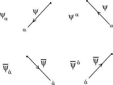
Figure 1: Weyl fermions.

We encode them as follows. We use 2 dimensional array with the size 2$\times$2. The four chiral spinors are stored in C-program as the array psi[ ][ ].

Fermionic Fields
(1) (Weyl) Spinor [Symbol: p ; Dimension: M^3/2 ]
$\psi^{\alpha}$ psi[0,0]=$\alpha$ psi[0,1]=empty psi[1,0]=empty psi[1,1]=empty   $\psi_{\alpha}$ psi[0,0]=empty psi[0,1]=$\alpha$ psi[1,0]=empty psi[1,1]=empty   ${\bar{\psi}}_{\dot{\alpha}}$ psi[0,0]=empty psi[0,1]=empty psi[1,0]=empty psi[1,1]=${\dot{\alpha}}$   ${\bar{\psi}}^{\dot{\alpha}}$ psi[0,0]=empty psi[0,1]=empty psi[1,0]=${\dot{\alpha}}$ psi[1,1]=empty

The first column takes two numbers 0 and 1; 0 expresses a ’chiral’ operator $\psi$, while 1 expresses an ’anti-chiral’ operator ${\bar{\psi}}$. The second column also takes the two numbers; 0 expresses an ’up’ suffix, while 1 expresses an ’down’ one.

Note: Chiral spinor suffixes $\alpha,\beta,\cdots$ are expressed , in the present C-program, by positive odd number integers 1,3,$\cdots$, while anti-chiral ones ${\dot{\alpha}},{\dot{\beta}},\cdots$ are by positive even number integers 2,4,$\cdots$. This convension (discriminative use of even and odd integers) is, at this stage, rather redundant in the sense that the chirality ($\psi$ or ${\bar{\psi}}$) can be read by the first element number of the array psi[2][2] for a non-empty data, i.e. 0 for $\psi$ (psi[0][*]=$\alpha$) and 1 for ${\bar{\psi}}$ (psi[1][*]=${\dot{\alpha}}$). (The situation is the same for some other spinors $\partial_{m}\psi,\theta,\cdots$. See the later discription. ) The convension, however, will soon become important to discriminate the chirality of the spinor matrices; $\sigma$ and ${\bar{\sigma}}$.

Note: ’empty’ is expressed by a default number (, for example, 99) in the program.

(2) First derivative of spinor [Symbol: q ; Dimension: M^5/2 ]
 The first derivative of the spinor is graphically expressed by the upper graph of Fig.2.

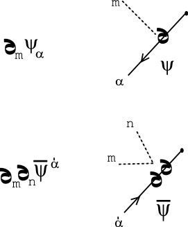
Figure 2: Derivatives of fermions.

It is stored by one 2$\times$2 array dps[ ][ ] and one variable dpsv.
$\partial_{m}\psi^{\alpha}$ dps[0,0]=$\alpha$ dps[0,1]=empty dps[1,0]=empty dps[1,1]=empty dpsv=m   $\partial_{m}\psi_{\alpha}$ dps[0,0]=empty dps[0,1]=$\alpha$ dps[1,0]=empty dps[1,1]=empty dpsv=m   $\partial_{m}{\bar{\psi}}_{\dot{\alpha}}$ dps[0,0]=empty dps[0,1]=empty dps[1,0]=empty dps[1,1]=${\dot{\alpha}}$ dpsv=m   $\partial_{m}{\bar{\psi}}^{\dot{\alpha}}$ dps[0,0]=empty dps[0,1]=empty dps[1,0]=${\dot{\alpha}}$ dps[1,1]=empty dpsv=m

Here the vector suffix expresses the Lorents suffix of a differetial operator.

Note: The vector suffixes m, n, $\cdots$ are expressed by 51, 52, $\cdots$ in the present program.

(3) Sigma Matrix [Symbol: s ; Dimension: M⁰ ]
 Sigma matrices $\sigma^{m},{\bar{\sigma}}^{m}$ are graphically expressed in Fig.3.

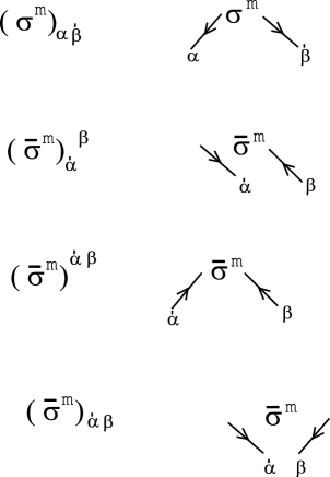
Figure 3: Elements of SL(2,C) $\sigma$-matrices. $(\sigma^{m})_{\alpha{\dot{\beta}}}$ and $({\bar{\sigma}}^{m})^{{\dot{\alpha}}\beta}$ are the standard form.

They are stored as the 2$\times$2 array si[ ][ ].
$\sigma^{m}_{\leavevmode\nobreak\ \alpha{\dot{\alpha}}}$ si[0,0]=empty si[0,1]=$\alpha$ si[1,0]=empty si[1,1]=${\dot{\alpha}}$ siv=m   ${\bar{\sigma}}^{m{\dot{\alpha}}\alpha}$ si[0,0]=${\dot{\alpha}}$ si[0,1]=empty si[1,0]=$\alpha$ si[1,1]=empty siv=m

Note: The use of even ($\alpha$) and odd (${\dot{\alpha}}$) integers makes an important role here. The arrangement of spinor suffixes, that is (left-side suffix, right-side suffix)=(odd, even) or (even, odd), makes us clear the difference between $\sigma$ and ${\bar{\sigma}}$. We should, however, have the relation

$${\bar{\sigma}}^{m}_{{\dot{\alpha}}\alpha}=\sigma^{m}_{\alpha{\dot{\alpha}}}$$

in mind. Hence the above 2quantities are equivelently expressed as
${\bar{\sigma}}^{m}_{\leavevmode\nobreak\ {\dot{\alpha}}\alpha}$ si[0,0]=empty si[0,1]=${\dot{\alpha}}$ si[1,0]=empty si[1,1]=$\alpha$ siv=m   $\sigma^{m\alpha{\dot{\alpha}}}$ si[0,0]=$\alpha$ si[0,1]=empty si[1,0]=${\dot{\alpha}}$ si[1,1]=empty siv=m
This ambiguity does not cause any problem because we keep a rule:

• In this program, we use only $\sigma$ (not use ${\bar{\sigma}}^{m}$).
  

• ${\bar{\sigma}}^{m}$ is used only for the graphical explanation.

(4) Superspace coordinate [Symbol: t ; Dimension: M^-1/2 ]
The superspace coordinate $\theta^{\alpha}$ is exprssed in the same way as the spinor $\psi^{\alpha}$.

$\theta^{\alpha}$ th[0,0]=$\alpha$ th[0,1]=empty th[1,0]=empty th[1,1]=empty   $\theta_{\alpha}$ th[0,0]=empty th[0,1]=$\alpha$ th[1,0]=empty th[1,1]=empty   ${\bar{\theta}}_{\dot{\alpha}}$ th[0,0]=empty th[0,1]=empty th[1,0]=empty th[1,1]=${\dot{\alpha}}$   ${\bar{\theta}}^{\dot{\alpha}}$ th[0,0]=empty th[0,1]=empty th[1,0]=${\dot{\alpha}}$ th[1,1]=empty
They are graphically expressed by Fig.4.

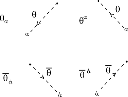
Figure 4: The graphical representation for the spinor coordinates in the superspace: $\theta_{\alpha},\theta^{\alpha},{\bar{\theta}}_{\dot{\alpha}}$ and ${\bar{\theta}}^{\dot{\alpha}}$.

(5) Gagino [Symbol: l ; Dimension: M^3/2 ]
The photino $\lambda^{\alpha}$ is exprssed in the same way as the spinor $\psi^{\alpha}$. We take the 2$\times$2 array la[ ][ ].

$\lambda^{\alpha}$ la[0,0]=$\alpha$ la[0,1]=empty la[1,0]=empty la[1,1]=empty   $\lambda_{\alpha}$ la[0,0]=empty la[0,1]=$\alpha$ la[1,0]=empty la[1,1]=empty   ${\bar{\lambda}}_{\dot{\alpha}}$ la[0,0]=empty la[0,1]=empty la[1,0]=empty la[1,1]=${\dot{\alpha}}$   ${\bar{\lambda}}^{\dot{\alpha}}$ la[0,0]=empty la[0,1]=empty la[1,0]=${\dot{\alpha}}$ la[1,1]=empty

(6) The first derivative of gaugino [Symbol: m ; Dimension: M^5/2 ]
The first derivative of the photino is expressed as the 2$\times$2 array dl[ ][ ] and the variable dlv.
$\partial_{m}\lambda^{\alpha}$ dl[0,0]=$\alpha$ dl[0,1]=empty dl[1,0]=empty dl[1,1]=empty dlv=m   $\partial_{m}\lambda_{\alpha}$ dl[0,0]=empty dl[0,1]=$\alpha$ dl[1,0]=empty dl[1,1]=empty dlv=m   $\partial_{m}{\bar{\lambda}}_{\dot{\alpha}}$ dl[0,0]=empty dl[0,1]=empty dl[1,0]=empty dl[1,1]=${\dot{\alpha}}$ dlv=m   $\partial_{m}{\bar{\lambda}}^{\dot{\alpha}}$ dl[0,0]=empty dl[0,1]=empty dl[1,0]=${\dot{\alpha}}$ dl[1,1]=empty dlv=m

Bosonic Fields
(7) Complex scalar [Symbol: A ; Dimension: M¹ ]
The complex scalar field $A$ is expressed by one dimensional array A[ ] with 2 elements.
A A[0]=1(exist) A[1]=empty   A^∗ A[0]=empty A[1]=1(exist)
where the element-numbers 0,1 correspond to $A$(chiral) or $A^{*}$(anti-chiral), respectively.

(8) The first derivative of the complex scalar [Symbol: B ; Dimension: M² ]
The first derivative of $A$ and $A^{*}$ are expressed as the one dimensional array B[ ] with 2 elements.
$\partial_{m}$A B[0]=m B[1]=empty   $\partial_{m}$A^∗ B[0]=empty B[1]=m

(9) Vector field [Symbol: v ; Dimension: M¹ ]
The vector field(photon) $v^{m}$ is expressed by one variable v.

$v^{m}$ v=m v=empty(non-exist)
The lowest expression is taken when the vector field does not appear.

(10) The first derivative of the vector field [Symbol: w ; Dimension: M² ]
The first derivative of $v^{m}$ is expressed by two variables dv and dvv.

$\partial_{n}v_{m}$ dv=m dvv=n

(11) The Dalemberian derivative of A and A^∗ [Symbol: C ; Dimension: M³ ]
The Dalemberian derivative of $A$ and $A^{*}$ are expressed as the one dimensional array C[ ] with 2 elements.
$\partial_{m}\partial^{m}$A C[0]=1(exist) C[1]=empty   $\partial_{m}\partial^{m}$A^∗ C[0]=empty C[1]=1(exist)

(12) Auxiliary fields [Symbol: F ; Dimension: M² ]
The auxiliary fields $F$ and $F^{*}$ are expressed as
F F[0]=1(exist) F[1]=empty   F^∗ F[0]=empty F[1]=1(exist)

(13) Real auxilary fields [Symbol: D ; Dimension: M² ]
The auxiliary field $D$ (real scalar), which appears in the vector multiplet, is expressed as
D D=1(exist) D=empty(non-exist)

Term and Component

Terms in the SUSY calculation are stored as an ordered set of the above quantities. The following examples appear in the intermidiate stage of evaluating $W_{\alpha}W^{\alpha}$ where $W_{\alpha}$ is the field strength superfield. (See App.B.)

Example 1

The term $\sigma^{l}_{\delta{\dot{\alpha}}}\sigma^{m\beta{\dot{\alpha}}}\sigma^{s\delta}_{\leavevmode\nobreak\ \ {\dot{\gamma}}}\sigma^{n\ {\dot{\gamma}}}_{\leavevmode\nobreak\ \beta}\partial_{l}v_{m}\partial_{s}v_{n}$= $-\sigma^{l}_{\delta{\dot{\alpha}}}{\bar{\sigma}}^{m{\dot{\alpha}}\beta}\sigma^{n}_{\beta{\dot{\gamma}}}{\bar{\sigma}}^{s{\dot{\gamma}}\delta}\partial_{l}v_{m}\partial_{s}v_{n}$ is stored, in the computer, as follows.
type[c=0]=s si[c=0,0,1]=1 si[c=0,1,1]=2 siv[c=0]=51   type[c=1]=s si[c=1,0,0]=3 si[c=1,1,0]=2 siv[c=1]=52   type[c=2]=s si[c=2,0,0]=1 si[c=2,1,1]=4 siv[c=2]=53   type[c=3]=s si[c=3,0,1]=3 si[c=3,1,0]=4 siv[c=3]=54   conti- nued below

type[c=4]=w dv[c=4]=52 dvv[c=4]=51   type[c=5]=w dv[c=5]=54 dvv[c=5]=53
($\delta\rightarrow 1,{\dot{\alpha}}\rightarrow 2,\beta\rightarrow 3,{\dot{\gamma}}\rightarrow 4;\ l\rightarrow 51,m\rightarrow 52,s\rightarrow 53,n\rightarrow 54$)
Besides the above ones, the number of components (compno=6) and an overall weight (complex) are necessary to characterize a term. One additional coloumn, specified by the variable c, appears. The variable c controls the order of every component. This ordering is important in the calculation involving Grassmannian quantities. In the above storing form, each component starts with specifying the type: s, w, $\cdots$. The one dimensional array type[ ] is used for the purpose. This term graphically appears in the output (before further reduction) as shown in Fig.5.

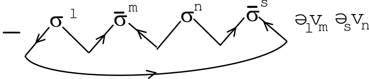
Figure 5: The graphical expression of $-\sigma^{l}_{\delta{\dot{\alpha}}}{\bar{\sigma}}^{m{\dot{\alpha}}\beta}\sigma^{n}_{\beta{\dot{\gamma}}}{\bar{\sigma}}^{s{\dot{\gamma}}\delta}\partial_{l}v_{m}\partial_{s}v_{n}$.

In Fig.5, we see all dummy suffixes disappear and the advantage of the graphical expression is manifest. The chirality can be read from the shape of the directed-line graph.

Example 2

The term $\sigma^{l\delta}_{\ {\dot{\alpha}}}\sigma^{m\leavevmode\nobreak\ {\dot{\alpha}}}_{\ \delta}D\partial_{l}v_{m}$= $-\sigma^{l}_{\delta{\dot{\alpha}}}{\bar{\sigma}}^{m{\dot{\alpha}}\delta}D\partial_{l}v_{m}$ is stored, in the computer, as follows.
type[c=0]=s si[c=0,0,0]=1 si[c=0,1,1]=4 siv[c=0]=53   type[c=1]=s si[c=1,0,1]=1 si[c=1,1,0]=4 siv[c=1]=54   type[c=2]=D D[c=2]=1   type[c=3]=w dv[c=3]=54 dvv[c=3]=53
($\delta\rightarrow 1,{\dot{\alpha}}\rightarrow 4;\ l\rightarrow 53,m\rightarrow 54$)
In this case, the number of components is 4 (compno=4) and there is a weight. This one graphically appears in the output (before further reduction) as shown in Fig.6.

Figure 6: The graphical expression of $-\sigma^{l}_{\delta{\dot{\alpha}}}{\bar{\sigma}}^{m{\dot{\alpha}}\delta}D\partial_{l}v_{m}$.

These two examples clearly show the advantage of the graph representation over the conventional one using indicies. The new representation discriminates each term not by the suffixes but by the shape of the graph. It means the importance of indices of the graph such as the number of the chiral-loop. (In the above examples, the number is 1.)

3 Field name, id-number and Grassmannian property

One advantage of C-language is the efficient manipulation of characters. The control of characters is important for specifying various operators (fields) appearing in SUSY theories. As described previously, we assign every operator a symbol which is expressed by a character. The appearance of many fields, which is a big cause complicating SUSY theories, can be neatly handled by the use of the character name. We also introduce the id-number for every operator. (See the list below)

For every operator, we assign the Grassmann number: +1(commuting) or -1(anti-commuting). This assignment is exploited in the process of moving a component , within a term, respecting the Grassmannian property of operators.

We list the assignment in TABLE 1 with the dimension of operators.

Fid[0]=’t’;	DIM[0]=0.0;	Grassmann[0]=-1;
Fid[1]=’s’;	DIM[1]=0.0;	Grassmann[1]=1;
/* <Chiral */
Fid[100]=’p’;	DIM[100]=(float)3/2;	Grassmann[100]=-1;
Fid[101]=’q’;	DIM[101]=(float)5/2;	Grassmann[101]=-1;
Fid[102]=’A’;	DIM[102]=1.0;	Grassmann[102]=1;
Fid[103]=’B’;	DIM[103]=2.0;	Grassmann[103]=1;
Fid[104]=’C’;	DIM[104]=3.0;	Grassmann[104]=1;
Fid[105]=’F’;	DIM[105]=2.0;	Grassmann[105]=1;
/* <Chiral2 */
Fid[120]=’P’;	DIM[120]=(float)3/2;	Grassmann[120]=-1;
Fid[121]=’Q’;	DIM[121]=(float)5/2;	Grassmann[121]=-1;
Fid[122]=’a’;	DIM[122]=1.0;	Grassmann[122]=1;
Fid[123]=’b’;	DIM[123]=2.0;	Grassmann[123]=1;
Fid[124]=’c’;	DIM[124]=3.0;	Grassmann[124]=1;
Fid[125]=’f’;	DIM[125]=2.0;	Grassmann[125]=1;
/* <Vector */
Fid[140]=’l’;	DIM[140]=(float)3/2;	Grassmann[140]=-1;
Fid[141]=’m’;	DIM[141]=(float)5/2;	Grassmann[141]=-1;
Fid[142]=’D’;	DIM[142]=2.0;	Grassmann[142]=1;
Fid[143]=’v’;	DIM[143]=1.0;	Grassmann[143]=1;
Fid[144]=’w’;	DIM[144]=2.0;	Grassmann[144]=1;
TABLE 1 Definition of FieldID, Dimension, Grassmann No

4 Graph Indices: vpairno, NcpairO, NcpairE, closed-chiral-loop-No, GrNum

SigmaContraction (B),(C),(D) and (E)

In the process of SUSY calculation, there appear graphs connected by directed lines (chiral suffixes contraction) and by (non-directed) dotted lines (vector suffixes contraction). We can classify them by some graph indices.

vpairno

The number of vector-suffix contractions.

NcpairO

The number of chiral-suffix contractions. This is equal to the number of left-directed wedges.

NcpairE

The number of anti-chiral-suffix contractions. This is equal to the number of the right-directed wedges.

closed-chiral-loop-No

The closed-chiral-loop is the case that the directed lines , connected by $\sigma$ or ${\bar{\sigma}}$, make a loop. In this case NcpairO=NcpairE. The number of closed chiral loops is defined to this index.

GrNum

A group is defined to be a set of $\sigma$’s or ${\bar{\sigma}}$’s which are connected by directed lines. The number of groups is defined to be GrNum.

In TABLE 2-4, we list the classification of the product of $\sigma$’s using the graph indices defined above.

vpairno	NcpairO	NcpairE	figure
	0	0	$\begin{array}[]{c}\mbox{ \includegraphics*[height=28.45274pt]{sig2Ar.eps} }\end{array}$
0	0	1	$\begin{array}[]{c}\mbox{ \includegraphics*[height=28.45274pt]{sig2Cr.eps} }\end{array}$
	1	0	$\begin{array}[]{c}\mbox{ \includegraphics*[height=28.45274pt]{sig2Cbr.eps} }\end{array}$
	1	1	$\begin{array}[]{c}\mbox{ \includegraphics*[height=28.45274pt]{sig2Dr.eps} }\end{array}\ =-2\eta^{mn}$
	0	0	$\begin{array}[]{c}\mbox{ \includegraphics*[height=28.45274pt]{sig2Br.eps} }\end{array}\ =-2\epsilon_{\alpha\beta}\epsilon_{{\dot{\alpha}}{\dot{\beta}}}$
1	0	1	$\begin{array}[]{c}\mbox{ \includegraphics*[height=28.45274pt]{sig2Fr.eps} }\end{array}\ =-4\delta^{\beta}_{\alpha}$
	1	0	$\begin{array}[]{c}\mbox{ \includegraphics*[height=28.45274pt]{sig2Fbr.eps} }\end{array}\ =-4\delta_{\dot{\beta}}^{\dot{\alpha}}$
	1	1	$\begin{array}[]{c}\mbox{ \includegraphics*[height=28.45274pt]{sig2Er.eps} }\end{array}\ =-8$
TABLE 2 Classification of the product of 2 sigma matrices (nsi=2).

vpairno	NcpairO	NcpairE	figure
	0	0	$\begin{array}[]{c}\mbox{ \includegraphics*[height=28.45274pt]{sig3Ar.eps} }\end{array}$
0	0	1	$\begin{array}[]{c}\mbox{ \includegraphics*[height=28.45274pt]{sig3Cbr.eps} }\end{array}$
	1	0	$\begin{array}[]{c}\mbox{ \includegraphics*[height=28.45274pt]{sig3Cr.eps} }\end{array}$
	1	1	closed-chiral-loop No =1 $\begin{array}[]{c}\mbox{ \includegraphics*[height=28.45274pt]{sig3Er.eps} }\end{array}$
			closed-chiral-loop No =0 $\begin{array}[]{c}\mbox{ \includegraphics*[height=28.45274pt]{sig3Gr.eps} }\end{array}$
	0	0	$-2\epsilon_{\alpha\beta}\epsilon_{{\dot{\alpha}}{\dot{\beta}}}\ \begin{array}[]{c}\mbox{ \includegraphics*[height=28.45274pt]{sig3Br.eps} }\end{array}$
1	0	1	$-4\delta^{\beta}_{\alpha}\ \begin{array}[]{c}\mbox{ \includegraphics*[height=28.45274pt]{sig3Dr.eps} }\end{array}$
	1	0	$-4\delta^{\dot{\alpha}}_{\dot{\beta}}\ \begin{array}[]{c}\mbox{ \includegraphics*[height=28.45274pt]{sig3Dr.eps} }\end{array}$
	1	1	$-8\ \begin{array}[]{c}\mbox{ \includegraphics*[height=28.45274pt]{sig3Fr.eps} }\end{array}$
TABLE 3 Classification of the product of 3 sigma matrices (nsi=3).

vpairno	NcpairO	NcpairE	figure
	0	0	$\begin{array}[]{c}\mbox{ \includegraphics*[height=28.45274pt]{sig4Ar.eps} }\end{array}$
	0	1	$\begin{array}[]{c}\mbox{ \includegraphics*[height=28.45274pt]{sig4Br.eps} }\end{array}$
	1	0	$\begin{array}[]{c}\mbox{ \includegraphics*[height=28.45274pt]{sig4Cr.eps} }\end{array}$
			GrNum=2, Division=(2,2) $\begin{array}[]{c}\mbox{ \includegraphics*[height=28.45274pt]{sig4Dr.eps} }\end{array}$
	1	1	GrNum=2, Division=(3,1) $\begin{array}[]{c}\mbox{ \includegraphics*[height=28.45274pt]{sig4Er.eps} }\end{array}$
			GrNum=3, Division=(2,1,1) $\begin{array}[]{c}\mbox{ \includegraphics*[height=28.45274pt]{sig4Fr.eps} }\end{array}$
0	2	0	$\begin{array}[]{c}\mbox{ \includegraphics*[height=28.45274pt]{sig4Gr.eps} }\end{array}$
	0	2	$\begin{array}[]{c}\mbox{ \includegraphics*[height=28.45274pt]{sig4Hr.eps} }\end{array}$
	1	2	GrNum=1, $\begin{array}[]{c}\mbox{ \includegraphics*[height=28.45274pt]{sig4Ir.eps} }\end{array}$
			GrNum=2, $\begin{array}[]{c}\mbox{ \includegraphics*[height=28.45274pt]{sig4Jr.eps} }\end{array}$
	2	1	GrNum=1, $\begin{array}[]{c}\mbox{ \includegraphics*[height=28.45274pt]{sig4Kr.eps} }\end{array}$
			GrNum=2, $\begin{array}[]{c}\mbox{ \includegraphics*[height=28.45274pt]{sig4Lr.eps} }\end{array}$
	2	2	GrNum=1, $\begin{array}[]{c}\mbox{ \includegraphics*[height=28.45274pt]{ssbssbBR.eps} }\end{array}$
			GrNum=2, $\begin{array}[]{c}\mbox{ \includegraphics*[height=28.45274pt]{sig4Mr.eps} }\end{array}$
TABLE 4 Classification of the product of 4 sigma matrices with
no vector-suffix contraction (nsi=4, vpairno=0).

These tables clearly show the $\sigma$-matrices play an important role to connect the chiral world and the space-time (Lorentz) world.

5 Superspace coordinates

Supersymmetry is most manifestly expressed in the superspace $(x^{m},\theta,{\bar{\theta}})$. $\theta_{\alpha}=\epsilon_{\alpha\beta}\theta^{\beta}$, ${\bar{\theta}}^{\dot{\alpha}}=\epsilon^{{\dot{\alpha}}{\dot{\beta}}}{\bar{\theta}}_{\dot{\beta}}$ are spinorial coordinates. They satisfy the relations graphically shown in Fig.7.

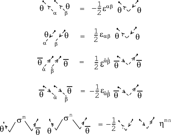
Figure 7: The graphical rules for the spinor coordinates: $\theta^{\alpha}\theta^{\beta}=-{\frac{1}{2}}\epsilon^{\alpha\beta}\theta\theta,\leavevmode\nobreak\ \theta_{\alpha}\theta_{\beta}={\frac{1}{2}}\epsilon_{\alpha\beta}\theta\theta,\leavevmode\nobreak\ {\bar{\theta}}^{\dot{\alpha}}{\bar{\theta}}^{\dot{\beta}}={\frac{1}{2}}\epsilon^{{\dot{\alpha}}{\dot{\beta}}}{\bar{\theta}}{\bar{\theta}},\leavevmode\nobreak\ {\bar{\theta}}_{\dot{\alpha}}{\bar{\theta}}_{\dot{\beta}}=-{\frac{1}{2}}\epsilon_{{\dot{\alpha}}{\dot{\beta}}}{\bar{\theta}}{\bar{\theta}},\leavevmode\nobreak\ \theta\sigma^{m}{\bar{\theta}}\theta\sigma^{n}{\bar{\theta}}=-{\frac{1}{2}}\theta\theta{\bar{\theta}}{\bar{\theta}}\eta^{mn}$.

These relations are exploited in the program in order to sort the SUSY quantities with respect to the power of $\theta\theta$ and ${\bar{\theta}}{\bar{\theta}}$. ( For further detail, see the subsection thBthBthth of App.A. )

6 Treatment of Metrics: $\epsilon_{\alpha\beta}$, $\epsilon_{\alpha}^{\leavevmode\nobreak\ \beta}=\epsilon^{\beta}_{\leavevmode\nobreak\ \alpha}=\delta_{\alpha}^{\beta}$, $\eta^{mn}$ and the totally anti-symmetric tensor $\epsilon^{lmns}$

For the totally anti-symmetric tensor $\epsilon^{lmns}$, we introduce one dimensional array ep[ ] with 4 components.

    ep[0]=l ep[1]=m ep[2]=n ep[3]=s     Symbol:  e    

This term appears in Sec.7 and produces topologically important terms such as $v_{lm}{\tilde{v}}^{lm}=\epsilon^{lmns}v_{lm}v_{ns}$.

As for the metric of the chiral suffix, we do not introduce specific arrays. They play a role of raising or lowering suffixes, which can be encoded in the upper (0) and lower (1) code in arrays. For the Lorentz metric $\eta^{mn}$, we do not need to much care for the discrimination between the upper and lower suffixes because of the even-symmetry with respect to the change of the Lorentz suffixes($\eta^{mn}=\eta^{nm}$).

7 Sigma matrices

Let us express important relations valid between products of sigma matrices graphically. In Fig.8, the symmetric combination of ${\bar{\sigma}}^{m}\sigma^{n}$ are shown as the basic spinor algebra.

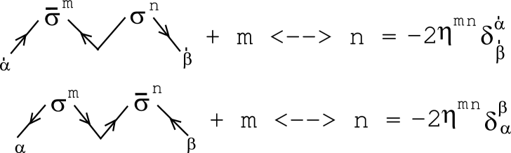
Figure 8: A graphical formula of the basic spinor algebra. $({\bar{\sigma}}^{m})^{{\dot{\alpha}}\beta}(\sigma^{n})_{\beta{\dot{\beta}}}+m\leftrightarrow n=-2\eta^{mn}\delta^{\dot{\alpha}}_{\dot{\beta}}$, and $(\sigma^{m})_{\alpha{\dot{\alpha}}}({\bar{\sigma}}^{n})^{{\dot{\alpha}}\beta}+m\leftrightarrow n=-2\eta^{mn}\delta^{\beta}_{\alpha}$.

The antisymmetric combination gives the generators of the Lorentz group, $\sigma^{nm},{\bar{\sigma}}^{nm}$.

$$(\sigma^{nm})_{\alpha}^{\leavevmode\nobreak\ \beta}=\frac{1}{4}\left\{\begin{array}[]{c}\mbox{ \includegraphics*[height=28.45274pt]{F1def2.eps} }\end{array}-m\leftrightarrow n\right\}{\quad,}$$ (8)

$$({\bar{\sigma}}^{nm})^{\dot{\alpha}}_{\leavevmode\nobreak\ {\dot{\beta}}}=\frac{1}{4}\left\{\begin{array}[]{c}\mbox{ \includegraphics*[height=28.45274pt]{F2def2.eps} }\end{array}-m\leftrightarrow n\right\}{\quad,}$$ (10)

The "reduction" formulae (from the cubic $\sigma^{\prime}$s to the linear one) are expressed as in Fig.9.

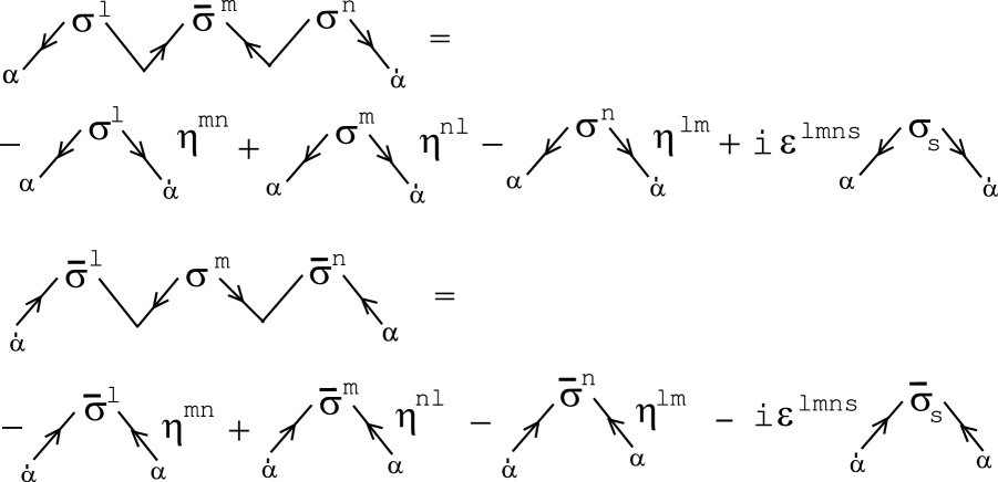
Figure 9: Two relations: 1) $\sigma^{l}{\bar{\sigma}}^{m}\sigma^{n}=-\sigma^{l}\eta^{mn}+\sigma^{m}\eta^{nl}-\sigma^{n}\eta^{lm}+i\epsilon^{lmns}\sigma_{s}$, 2) ${\bar{\sigma}}^{l}\sigma^{m}{\bar{\sigma}}^{n}=-{\bar{\sigma}}^{l}\eta^{mn}+{\bar{\sigma}}^{m}\eta^{nl}-{\bar{\sigma}}^{n}\eta^{lm}-i\epsilon^{lmns}{\bar{\sigma}}_{s}$.

From Fig.9, we notice any chain of $\sigma^{\prime}$s can always be expressed by less than three $\sigma^{\prime}$s. The appearance of the 4th rank anti-symmetric tensor $\epsilon^{lmns}$ is quite illuminating. The completeness relations are expressed as in Fig.10.

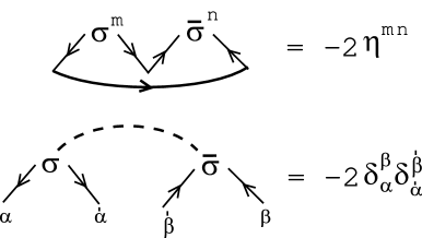
Figure 10: Completeness relations: 1) $\delta^{\alpha}_{\beta}(\sigma^{m})_{\alpha{\dot{\alpha}}}({\bar{\sigma}}^{n})^{{\dot{\alpha}}\beta}=-2\eta^{mn}$, 2) $(\sigma^{m})_{\alpha{\dot{\alpha}}}({\bar{\sigma}}_{m})^{{\dot{\beta}}\beta}=-2\delta^{\beta}_{\alpha}\delta^{\dot{\beta}}_{\dot{\alpha}}$. The contraction using $\delta^{\alpha}_{\beta}$ is the matrix trace. The relation 1) is also obtained from Fig.8.

The contraction, expressed by arrowed curve in Fig.10.is the matrix trace.

Fierz identity is graphically shown as follows.

$$\begin{array}[]{c}\mbox{ \includegraphics*[height=28.45274pt]{F1fierz.eps} }\end{array}=$$ (12)

$$\frac{1}{4}\left\{-\begin{array}[]{c}\mbox{ \includegraphics*[height=28.45274pt]{F2fierz.eps} }\end{array}\epsilon_{{\dot{\alpha}}{\dot{\beta}}}+\begin{array}[]{c}\mbox{ \includegraphics*[height=28.45274pt]{F3fierz.eps} }\end{array}\epsilon_{\alpha\beta}-m\leftrightarrow n\right\}$$ (15)

$$-{\frac{1}{2}}\eta^{nm}\epsilon_{\alpha\beta}\epsilon_{{\dot{\alpha}}{\dot{\beta}}}-\frac{1}{8}\left\{\begin{array}[]{c}\mbox{ \includegraphics*[height=28.45274pt]{F4fierz.eps} }\end{array}-l\leftrightarrow n\right\}\left\{\begin{array}[]{c}\mbox{ \includegraphics*[height=28.45274pt]{F5fierz.eps} }\end{array}-l\leftrightarrow m\right\},$$ (18)

These relations are important, in the program, to reduce the product of sigma matrices. Especially at the place (E) of SigmaContraction, they are exploited. As an example, the closed chiral-loop graph in Fig.5 reduces as follows.

$$\begin{array}[]{c}\mbox{ \includegraphics*[height=28.45274pt]{ssbssbBR.eps} }\end{array}=2(\eta^{lm}\eta^{ns}-\eta^{ln}\eta^{ms}+\eta^{ls}\eta^{mn}-i\epsilon^{lmns})$$ (20)

Its complex conjugate one is given by

$$\begin{array}[]{c}\mbox{ \includegraphics*[height=28.45274pt]{sbssbsR.eps} }\end{array}=2(\eta^{lm}\eta^{ns}-\eta^{ln}\eta^{ms}+\eta^{ls}\eta^{mn}+i\epsilon^{lmns})$$ (22)

The above 2 terms appear in the calculation of $W_{\alpha}W^{\alpha}$ and ${\bar{W}}_{\dot{\alpha}}{\bar{W}}^{\dot{\alpha}}$ respectively. ($W_{\alpha}$ and ${\bar{W}}_{\dot{\alpha}}$ are superfields of field strength. )

8 Superfield and Structure of Input Data

The transformation between the superfield expression and the fields-components expression is an important subject of SUSY theories. For the purpose, we do the calculation of $\Phi^{\dagger}\Phi$, in the App.B. In this case, the input data is taken from the content of the superfield. The first superfield $\Phi^{\dagger}$(we assign the superfield-number sf=0) and the second one $\Phi$(sf=1) have 6 terms (we assign the term-number t=0,1,$\cdots$,5) within each superfield. The input data, written in App.B, can be read from the following expression.

$$\Phi^{\dagger}=-i\begin{array}[]{c}\mbox{ \includegraphics*[height=28.45274pt]{PHI1r.eps} }\end{array}\partial_{m}A^{*}+\begin{array}[]{c}\mbox{ \includegraphics*[height=28.45274pt]{PHI2r.eps} }\end{array}\frac{1}{4}\partial^{2}A^{*}+2\begin{array}[]{c}\mbox{ \includegraphics*[height=28.45274pt]{PHIB3r.eps} }\end{array}$$ (26)

$$+i\begin{array}[]{c}\mbox{ \includegraphics*[height=28.45274pt]{PHIB4r.eps} }\end{array}+\begin{array}[]{c}\mbox{ \includegraphics*[height=28.45274pt]{PHIB5r.eps} }\end{array}F^{*}+A^{*}$$ (29)

This data of $\Phi^{\dagger}$ is stored as

weight[sf=0,t=0]=0+i(-1) type[sf=0,t=0,c=0]= t th[sf=0,t=0,c=0,0,0]=1 type[sf=0,t=0,c=1]= s si[sf=0,t=0,c=1,0,1]=1 si[sf=0,t=0,c=1,1,1]=2 siv[sf=0,t=0,c=1]=51 type[sf=0,t=0,c=2]= t th[sf=0,t=0,c=2,1,0]=2 type[sf=0,t=0,c=3]= B B[sf=0,t=0,c=3,1]=51 weight[sf=0,t=1]=1+i(0) type[sf=0,t=1,c=0]= t th[sf=0,t=1,c=0,0,0]=1 type[sf=0,t=1,c=1]= t th[sf=0,t=1,c=1,0,1]=1 type[sf=0,t=1,c=2]= t th[sf=0,t=1,c=2,1,1]=2 type[sf=0,t=1,c=3]= t th[sf=0,t=1,c=3,1,0]=2 type[sf=0,t=1,c=4]= C C[sf=0,t=1,c=4,1]=1

$\cdot\cdot\cdot$

Here we notice two additional coloumns, specified by sf and t, appear. They specify the order of the supersields and the order of the terms within each superfield respectively.

The superfield $\Phi$ is graphically shown as

$$\Phi=i\begin{array}[]{c}\mbox{ \includegraphics*[height=28.45274pt]{PHI1r.eps} }\end{array}\partial_{m}A+\begin{array}[]{c}\mbox{ \includegraphics*[height=28.45274pt]{PHI2r.eps} }\end{array}\frac{1}{4}\partial^{2}A+2\begin{array}[]{c}\mbox{ \includegraphics*[height=28.45274pt]{PHI3r.eps} }\end{array}$$ (33)

$$-i\begin{array}[]{c}\mbox{ \includegraphics*[height=28.45274pt]{PHI4r.eps} }\end{array}+\begin{array}[]{c}\mbox{ \includegraphics*[height=28.45274pt]{PHI5r.eps} }\end{array}F+A$$ (36)

This data of $\Phi$ is stored as
weight[sf=1,t=0]=0+i(1) type[sf=1,t=0,c=0]= t th[sf=1,t=0,c=0,0,0]=5 type[sf=1,t=0,c=1]= s si[sf=1,t=0,c=1,0,1]=5 si[sf=1,t=0,c=1,1,1]=6 siv[sf=1,t=0,c=1]=52 type[sf=1,t=0,c=2]= t th[sf=1,t=0,c=2,1,0]=6 type[sf=1,t=0,c=3]= B B[sf=1,t=0,c=3,0]=52   weight[sf=1,t=1]=1+i(0) type[sf=1,t=1,c=0]= t th[sf=1,t=1,c=0,0,0]=5 type[sf=1,t=1,c=1]= t th[sf=1,t=1,c=1,0,1]=5 type[sf=1,t=1,c=2]= t th[sf=1,t=1,c=2,1,1]=6 type[sf=1,t=1,c=3]= t th[sf=1,t=1,c=3,1,0]=6 type[sf=1,t=1,c=4]= C C[sf=1,t=1,c=4,0]=1  $\cdot\cdot\cdot$

The calculation of $\Phi{\dagger}\Phi$ leads to the Wess-Zumino Lagrangian. (See App.B)

We also do the calculation of $W_{\alpha}W^{\alpha}$ in App.B where $W_{\alpha}$ is the field strength superfield. They are expressed as follows.

$$W_{\alpha}=-i\begin{array}[]{c}\mbox{ \includegraphics*[height=28.45274pt]{WalD1r.eps} }\end{array}+\begin{array}[]{c}\mbox{ \includegraphics*[height=28.45274pt]{WalD2r.eps} }\end{array}D-i\begin{array}[]{c}\mbox{ \includegraphics*[height=28.45274pt]{WalD3r.eps} }\end{array}{\frac{1}{2}}v_{mn}+\begin{array}[]{c}\mbox{ \includegraphics*[height=28.45274pt]{WalD4r.eps} }\end{array}$$ (41)

This data of $W_{\alpha}$ is stored as

weight[sf=0,t=0]=0+i(-1) type[sf=0,t=0,c=0]= l la[sf=0,t=0,c=0,0,1]=1 weight[sf=0,t=1]=1+i(0) type[sf=0,t=1,c=0]= t th[sf=0,t=1,c=0,0,1]=1 type[sf=0,t=1,c=1]= D D[sf=0,t=1,c=1]=1

$\cdot\cdot\cdot$

$W^{\alpha}$ is expressed as

$$W^{\alpha}=-i\begin{array}[]{c}\mbox{ \includegraphics*[height=28.45274pt]{WalU1r.eps} }\end{array}+\begin{array}[]{c}\mbox{ \includegraphics*[height=28.45274pt]{WalU2r.eps} }\end{array}D-i\begin{array}[]{c}\mbox{ \includegraphics*[height=28.45274pt]{WalU3r.eps} }\end{array}{\frac{1}{2}}v_{mn}+\begin{array}[]{c}\mbox{ \includegraphics*[height=28.45274pt]{WalU4r.eps} }\end{array}$$ (46)

This data of $W^{\alpha}$ is stored as

weight[sf=1,t=0]=0+i(-1) type[sf=1,t=0,c=0]= l la[sf=1,t=0,c=0,0,0]=1 weight[sf=1,t=1]=1+i(0) type[sf=1,t=1,c=0]= t th[sf=1,t=1,c=0,0,0]=1 type[sf=1,t=1,c=1]= D D[sf=1,t=1,c=1]=1

$\cdot\cdot\cdot$
The calculation of $W_{\alpha}W^{\alpha}$ leads to the Super Electromagnetism Lagrangian.(See App.B)

9 Conclusion

In the history of the quantum field theory, new techniques have produced physically important results. The regularization techniques are such examples. The dimensional regularization by ’tHooft and Veltman[5] produced important results on the renormalization group property of Yang-Mills theory and many scattering amplitude calculations. The lattice regularization in the gauge theory revealed non-perturbative features of hadron physics. In this case, the computor technique of numerical calculation is essential. As for the computer algebraic one, we recall the calculation of 2-loop on-shell counterterms of pure Einstein gravity[6, 7]. A new technique is equally important as a new idea.

The SUSY theory is beautifully constructed respecting the symmetry between bosons and fermions, but the attractiveness is practically much reduced by its complicated structure: many fields, chiral properties, Grassmannian algebra, etc. The present approach intends to improve the situation by a computer program which makes use of the graphical technique. (This approach is taken in Ref.[8] for the calculation of product of SO(N) tensors. It was applied to various anomaly calculations. )

The present program should be much more improved. Here we cite the prospective final goal.

1. It can do the transformation between the superfield expression and the component expression.

2. It can do the SUSY trnasformation of various quantities. In particular it can confirm the SUSY-invariance of the Lagrangian in the graphical way and give the final total divergence.

3. It can do algebraic SUSY calculation involving $D_{\alpha},{\bar{D}}^{\dot{\alpha}},Q_{\alpha}$ and ${\bar{Q}}^{\dot{\alpha}}$.

The item 1 above has been demostrated in the present paper.

It is impossible to deal with all SUSY calculations. This is simply because which fields appear and which dimensional quantities are calculated depend on each problem. If we obatin a list of (graph) indices which classify all phsical quantities (operators) appearing in the output, then the present program works (by adding new lines for the new problem). To deal with such a case, we add the appendix B where the program flow is explained. It intends to help the reader to read the original source code.

10 Appendix A: Skech of Programming Flow

10.1 Input of Data

[Install of SuperField Data]

} /* c-running> */
} /* t-running> */
} /* sf-running> */

/* Expanding the product of superfields */

10.2 termscombine

printf("*** TERMSCOMBINE ***");

10.3 SORTOUTthBth

Moving th($\theta$), thbar(${\bar{\theta}}$), si($\sigma$) and sibar(${\bar{\sigma}}$) to the biggining part of a term. In the process, we obtain the sign change due to the Grassman algebra.

idno(TP); a function which produces FieldID number correponding to a type TP.

10.4 thBthBthth

First we change the data form of th[ ][ ][ ]. From :

In this part, the program classifies terms by the power of $\theta$ and ${\bar{\theta}}$.
(1) indipendent of $\theta$ and ${\bar{\theta}}$ (nth=0)
(2) $\theta^{\alpha},\theta_{\alpha},{\bar{\theta}}_{\dot{\alpha}},{\bar{\theta}}^{\dot{\alpha}}$ (nth=1)
(3) $\theta^{\alpha}{\bar{\theta}}^{\dot{\beta}},\theta^{\alpha}{\bar{\theta}}_{\dot{\beta}},\cdots$ (nth=2)
(4) $\theta^{\alpha}\theta^{\beta},\theta^{\alpha}\theta_{\beta},\cdots;{\bar{\theta}}^{\dot{\alpha}}{\bar{\theta}}^{\dot{\beta}},{\bar{\theta}}^{\dot{\alpha}}{\bar{\theta}}_{\dot{\beta}},\cdots;\theta^{2};{\bar{\theta}}^{2}$ (nth=2)
(5) $\theta^{2}({\bar{\theta}}_{\dot{\alpha}},{\bar{\theta}}^{\dot{\alpha}}),{\bar{\theta}}^{2}(\theta_{\alpha},\theta^{\alpha})$ (nth=3)
(6) $\theta^{\alpha}\theta^{\beta}{\bar{\theta}}_{\dot{\gamma}},\cdots;{\bar{\theta}}^{\dot{\alpha}}{\bar{\theta}}^{\dot{\beta}}\theta_{\gamma},\cdots$ (nth=3)
(7) $\theta^{\alpha}{\bar{\theta}}^{\dot{\beta}}{\bar{\theta}}^{\dot{\gamma}}\theta^{\delta},\cdots;{\bar{\theta}}^{\dot{\alpha}}\theta^{\beta}\theta^{\gamma}{\bar{\theta}}^{\dot{\delta}},\cdots;\cdots$ (nth=4)
(8) $\theta^{\alpha}{\bar{\theta}}^{\dot{\beta}}\theta^{\gamma}{\bar{\theta}}^{\dot{\gamma}},\cdots;{\bar{\theta}}^{\dot{\alpha}}\theta^{\beta}{\bar{\theta}}^{\dot{\gamma}}\theta^{\delta},\cdots;\cdots$ (nth=4)
(9) $\theta^{\alpha}\theta^{\beta}{\bar{\theta}}^{\dot{\gamma}}{\bar{\theta}}^{\dot{\delta}},\cdots;{\bar{\theta}}^{\dot{\alpha}}{\bar{\theta}}^{\dot{\beta}}\theta^{\gamma}\theta^{\delta},\cdots;\cdots$ (nth=4)

The formula presented in Sec.5 is exploited here. As the output, we obtain

10.5 SigmaContraction

This routine is composed of 5 parts, (A),(B),(C),(D) and (E).

(A) Change of the data form
First we change the data form: (N=nsi-1)
$\sigma^{m_{0}}_{\alpha_{0}{\dot{\alpha}}_{0}}$   $\sigma^{m_{1}\alpha_{1}{\dot{\alpha}}_{1}}$  $\cdots$  $\sigma^{m_{N}\ {\dot{\alpha}}_{N}}_{\ \ \alpha_{N}}$
to an another form:
c=0   c=1  $\cdots$   c=N

(B) Chiral-suffix-pair search
Search for same suffixes in {Csuff[c][0]|c=0,1,$\cdots$,N}(odd number suffixes) and in {Csuff[c][1]|c=0,1,$\cdots$,N}(even number suffixes). When Csuff[c1][0]=Csuff[c2][0], then we call (c1,c2) chiral-suffix-pair (or, simply, Cpair). For the odd number case, we list them as

(C) Grouping $\sigma$’s
A group of $\sigma$’s is defined to be a set of $\sigma$’s which are connected by chiral-suffix or anti-chiral-suffix contractions. The number of groups within a term is assigned to be GrNum. This an important Graph index. The number of $\sigma$’s which each group has is stored in SigmaN[GR] (GR=0,1,$\cdots$,GrNum-1). Each group consits of some $\sigma$’s specified their component numbers. They are stored in Group[GR][nseries] (nseries=0,1,$\cdot$,SigmaN[GR]-1). In this process of grouping, the program traces the CpairO and CpairE defined in (B). Each group is determined by a series of cpairnoO’s and cpainoE’s. They are stored in CPseries[GR][ ].

(D) Vector-suffix-pair search
Search the same vector-suffix in {Vsuff[c]|c=0,1,$\cdots$,N}.

(E) Classifying $\sigma$’s part by indices (nsi, vpairno, NcpairO, NcpairE, closed chiral-loop)

Using graph indices defined in the Sec.4, we can classify $\sigma$’s part. See the TABLE 2,3 and 4 in the text. Each class (we call here the finally classified place "class") has the number SigGraN which is the set of the graph indices. In each class, we reduce the expression using the graphical relations explained in Sec.7. Here the following important data are obtained and transfered to VecSufChange().

BranchN: Generally each class decomposes to some branches after the reduction using the graphical relations. We specify the number of branches.
NoChangeN[br]: For each branch(br), NoChangeN is assigned, 0 for the case that $\sigma$’s part does not change, 1 for the case that $\sigma$’s part changes.
RedSigN[br]: For each branch, the decrease-number of $\sigma$’s after the reduction is stored. This number is important for adjusting the output form.
cstart: Normally this is fixed as cstart=nth+nsi
LorenContN[br]: For each branch, specify the number of Lorenz contraction, in other words, the number of $\eta^{mn}$.
SUFF[br][10][2]: Specify the vector suffixes appearing in $\eta$’s.
MultiFac[br][2]: For each branch, a multiplicative factor is specified.
si1BR[br][c][2][2], siv1BR[br][c]: For each branch, specify the $\sigma$’s part.
ep1[c][4]: For each branch, specify the totally-antisymmetric tensor when this term appears.

10.6 VecSufChange

Vector suffix contraction is peformed using $\eta^{mn}\eta^{ls}\cdots$. It is done for component c (c$\geq$cstart=nth+nsi).

10.6.1 FinalOutPut

11 Appendix B: Input and Output Examples

11.1 Wess-Zumino Model

We demonstrate the calculation of $\Phi^{\dagger}\Phi$, where $\Phi$ is the chiral superfield, and obtain the component form. The next input data can be read from the graphical eqauations (29) and (36).

INPUT DATA

2

6

0 -1 4 t 0 0 1 s 0 1 1 1 1 2 51 t 1 0 2 B 1 51

1 0 5 t 0 0 1 t 0 1 1 t 1 1 2 t 1 0 2 C 1 1

2 0 2 t 1 1 2 p 1 0 2

0 1 5 t 1 1 2 t 1 0 2 t 0 0 1 s 0 1 1 1 1 4 51 q 1 0 4 51

1 0 3 t 1 1 2 t 1 0 2 F 1 1

1 0 1 A 1 1

6

0 1 4 t 0 0 5 s 0 1 5 1 1 6 52 t 1 0 6 B 0 52

1 0 5 t 0 0 5 t 0 1 5 t 1 1 6 t 1 0 6 C 0 1

2 0 2 t 0 0 5 p 0 1 5

0 -1 5 t 0 0 5 t 0 1 5 q 0 0 7 52 s 0 1 7 1 1 6 52 t 1 0 6

1 0 3 t 0 0 5 t 0 1 5 F 0 1

1 0 1 A 0 1

OUT PUT

T[0]=0 T[1]=0

****** TERMSCOMBINE ****
th*th*thbar*thbar-term

****** SORTOUTthBth ****
lab50 at thBthBthth, Final result
weight= 1+i(0) PlusMinus= 0 Sign=2 Nthth=1 NthBthB=1 Nhalf=2

****** SigmaContraction ****
SigGraN=201199 FinalOutPut: MultiFac=-2 + i(0) type2[c=6]= B B2[c=6,1]=51 type2[c=7]= B B2[c=7,0]=51

T[0]=1 T[1]=5

****** TERMSCOMBINE ****
th*th*thbar*thbar-term

****** SORTOUTthBth ****
lab50 at thBthBthth, Final result
weight= 1+i(0) PlusMinus= 0 Sign=0 Nthth=1 NthBthB=1 Nhalf=0

****** SigmaContraction ****
SigGraN=0 FinalOutPut: MultiFac=1 + i(0) type2[c=4]= C C2[c=4,1]=1 type2[c=5]= A A2[c=5,0]=1

T[0]=2 T[1]=3

****** TERMSCOMBINE ****
th*th*thbar*thbar-term

****** SORTOUTthBth ****
lab50 at thBthBthth, Final result
weight= 0+i(-2) PlusMinus= 4 Sign=0 Nthth=1 NthBthB=1 Nhalf=1

****** SigmaContraction ****
SigGraN=1 FinalOutPut: MultiFac=1 + i(0) type2[c=4]= s si2[c=4,0,1]=7 si2[c=4,1,1]=2 siv2[c=4]=52 type2[c=5]= p psi2[c=5,1,0]=2 type2[c=6]= q dps2[c=6,0,0]=7 dpsv2[c=6]=52

T[0]=3 T[1]=2

****** TERMSCOMBINE ****
th*th*thbar*thbar-term

****** SORTOUTthBth **** lab50 at thBthBthth, Final result
weight= 0+i(2) PlusMinus= 1 Sign=1 Nthth=1 NthBthB=1 Nhalf=1

****** SigmaContraction ****
SigGraN=1 FinalOutPut: MultiFac=1 + i(0) type2[c=4]= s si2[c=4,0,1]=1 si2[c=4,1,1]=4 siv2[c=4]=51 type2[c=5]= q dps2[c=5,1,0]=4 dpsv2[c=5]=51 type2[c=6]= p psi2[c=6,0,0]=1

T[0]=4 T[1]=4

****** TERMSCOMBINE ****
th*th*thbar*thbar-term

****** SORTOUTthBth ****
lab50 at thBthBthth, Final result
weight= 1+i(0) PlusMinus= 0 Sign=0 Nthth=1 NthBthB=1 Nhalf=0

****** SigmaContraction ****
SigGraN=0 FinalOutPut: MultiFac=1 + i(0) type2[c=4]= F F2[c=4,1]=1 type2[c=5]= F F2[c=5,0]=1

T[0]=5 T[1]=1

****** TERMSCOMBINE ****
th*th*thbar*thbar-term

****** SORTOUTthBth ****
lab50 at thBthBthth, Final result
weight= 1+i(0) PlusMinus= 0 Sign=0 Nthth=1 NthBthB=1 Nhalf=0

****** SigmaContraction ****
SigGraN=0 FinalOutPut: MultiFac=1 + i(0) type2[c=4]= A A2[c=4,1]=1 type2[c=5]= C C2[c=5,0]=1

Gathering all terms, we obtain

$$\Phi^{\dagger}\Phi|_{\theta^{2}{\bar{\theta}}^{2}}==-{\frac{1}{2}}\partial_{m}A^{*}\partial^{m}A\ {\bf(0,0)}+\frac{1}{4}\partial^{2}A^{*}\cdot A\ {\bf(1,5)}+\frac{1}{4}A^{*}\partial^{2}A\ {\bf(5,1)}$$

$$-i\times(-1)\begin{array}[]{c}\mbox{ \includegraphics*[height=28.45274pt]{OutFig2r.eps} }\end{array}\ {\bf(2,3)}+i\times(-1)\begin{array}[]{c}\mbox{ \includegraphics*[height=28.45274pt]{OutFig1r.eps} }\end{array}\ {\bf(3,2)}+F^{*}F\ {\bf(4,4)}$$ (49)

This is the Wess-Zumino Lagrangian. We donot ignore the total divergence here.

11.2 Super QED

The calculation of $W_{\alpha}W^{\alpha}$ gives the kinetic terms of the photon and the photino in Super QED. The following input data can be read from the graphical eqauations (41) and (46).

INPUT DATA

2

4

0 -1 1 l 0 1 1

1 0 2 t 0 1 1 D 1

0 -1 4 s 0 1 1 1 1 2 51 s 0 0 3 1 0 2 52 t 0 1 3 w 52 51

1 0 4 t 0 0 3 t 0 1 3 s 0 1 1 1 1 2 51 m 1 0 2 51

4

0 -1 1 l 0 0 1

1 0 2 t 0 0 1 D 1

0 -1 4 s 0 0 1 1 1 4 53 s 0 0 5 1 0 4 54 t 0 1 5 w 54 53

1 0 4 t 0 0 5 t 0 1 5 s 0 0 1 1 1 4 53 m 1 0 4 53

OUT PUT

T[0]=0 T[1]=3

****** TERMSCOMBINE ****
th*th-term

****** SORTOUTthBth ****
lab50 at thBthBthth, Final result
weight= 0+i(-1) PlusMinus= 2 Sign=0 Nthth=1 NthBthB=0 Nhalf=0

****** SigmaContraction ****
SigGraN=1 FinalOutPut: MultiFac=1 + i(0) type2[c=2]= s si2[c=2,0,0]=1 si2[c=2,1,1]=4 siv2[c=2]=53 type2[c=3]= l la2[c=3,0,1]=1 type2[c=4]= m dl2[c=4,1,0]=4 dlv2[c=4]=53

T[0]=1 T[1]=1

****** TERMSCOMBINE ****
th*th-term

****** SORTOUTthBth ****
lab50 at thBthBthth, Final result
weight= 1+i(0) PlusMinus= 0 Sign=1 Nthth=1 NthBthB=0 Nhalf=0

****** SigmaContraction ****
SigGraN=0 FinalOutPut: MultiFac=1 + i(0) type2[c=2]= D D2[c=2]=1 type2[c=3]= D D2[c=3]=1

T[0]=1 T[1]=2

****** TERMSCOMBINE ****
th*th-term

****** SORTOUTthBth ****
lab50 at thBthBthth, Final result
weight= 0+i(-1) PlusMinus= 0 Sign=0 Nthth=1 NthBthB=0 Nhalf=1

****** SigmaContraction ****
SigGraN=201199 FinalOutPut: MultiFac=2 + i(0) type2[c=4]= D D2[c=4]=1 type2[c=5]= w dv2[c=5]=53 dvv2[c=5]=53

T[0]=2 T[1]=1

****** TERMSCOMBINE ****
th*th-term

****** SORTOUTthBth ****
lab50 at thBthBthth, Final result
weight= 0+i(-1) PlusMinus= 0 Sign=1 Nthth=1 NthBthB=0 Nhalf=1

****** SigmaContraction ****
SigGraN=201199 FinalOutPut: MultiFac=-2 + i(0) type2[c=4]= w dv2[c=4]=51 dvv2[c=4]=51 type2[c=5]= D D2[c=5]=1

T[0]=2 T[1]=2

****** TERMSCOMBINE ****
th*th-term

****** SORTOUTthBth ****
lab50 at thBthBthth, Final result
weight= -1+i(0) PlusMinus= 0 Sign=0 Nthth=1 NthBthB=0 Nhalf=1

****** SigmaContraction ****
SigGraN=402299
Branch No 0
FinalOutPut: MultiFac=-2 + i(0) type2[c=6]= w dv2[c=6]=51 dvv2[c=6]=51 type2[c=7]= w dv2[c=7]=54 dvv2[c=7]=54
Branch No 1
FinalOutPut: MultiFac=2 + i(0) type2[c=6]= w dv2[c=6]=52 dvv2[c=6]=51 type2[c=7]= w dv2[c=7]=51 dvv2[c=7]=52
Branch No 2
FinalOutPut: MultiFac=-2 + i(0) type2[c=6]= w dv2[c=6]=52 dvv2[c=6]=51 type2[c=7]= w dv2[c=7]=52 dvv2[c=7]=51
Branch No 3
FinalOutPut: MultiFac=0 + i(2) type2[c=5]= e ep(51,52,54,53) type2[c=6]= w dv2[c=6]=52 dvv2[c=6]=51 type2[c=7]= w dv2[c=7]=54 dvv2[c=7]=53

T[0]=3 T[1]=0

****** TERMSCOMBINE ****
th*th-term

****** SORTOUTthBth ****
lab50 at thBthBthth, Final result
weight= 0+i(-1) PlusMinus= 0 Sign=0 Nthth=1 NthBthB=0 Nhalf=0

****** SigmaContraction ****
SigGraN=1 FinalOutPut: MultiFac=1 + i(0) type2[c=2]= s si2[c=2,0,1]=1 si2[c=2,1,1]=2 siv2[c=2]=51 type2[c=3]= m dl2[c=3,1,0]=2 dlv2[c=3]=51 type2[c=4]= l la2[c=4,0,0]=1

Gathering all terms, we obtain

$$W_{\alpha}W^{\alpha}=2i\begin{array}[]{c}\mbox{ \includegraphics*[height=28.45274pt]{OutFig1r.eps} }\end{array}\ {\bf\{(0,3),(3,0)\}}\ +\ 0\ {\bf(1,2)}\ +\ 0\ {\bf(2,1)}$$ (51)

$$-{\frac{1}{2}}\left(0\ {\bf(2,2)br0}-{\frac{1}{2}}{v_{mn}}^{2}\ {\bf(2,2)br1}-{\frac{1}{2}}{v_{mn}}^{2}\ {\bf(2,2)br2}-2i\epsilon^{m,n,s,l}{\frac{1}{2}}v_{mn}\cdot{\frac{1}{2}}v_{sl}\ {\bf(2,2)br3}\right)$$

$$-D^{2}\ {\bf(1,1)}.$$ (52)

Adding ${\bar{W}}{\bar{W}}$, we obtain the Lagrangian as

$${\cal L}=\frac{1}{4}(-W_{\alpha}W^{\alpha}|_{\theta^{2}}+{\bar{W}}_{\dot{\alpha}}{\bar{W}}^{\dot{\alpha}}|_{{\bar{\theta}}^{2}})$$

$$=-\frac{1}{4}{v_{mn}}^{2}+\frac{i}{2}(\begin{array}[]{c}\mbox{ \includegraphics*[height=28.45274pt]{OutFig2r.eps} }\end{array}-\begin{array}[]{c}\mbox{ \includegraphics*[height=28.45274pt]{OutFig1r.eps} }\end{array})+{\frac{1}{2}}D^{2}\ ,$$ (55)

where we do not ignore the total divergence. This is the kinetic term of the photon and the photino.

References

- [1] S. Ichinose, hep-th/0301166, DAMTP-2003-8, US-03-01, "Graphical Representation of Supersymmetry"
- [2] S. Ichinose, hep-th/0410027, Proc. 12th Int.Conf. on "Supersymmetry and Unification of Fundamental Interactions"(June 17-23,2004,Epochal Tsukuba Congress Center,Japan), p853-856, "Graphical Representation of Supersymmetry and Computer Calculation"
- [3] S. Ichinose, Univ. Vienna preprint UWThPh-2006-7, "Graphical Representation of Supersymmetry"
- [4] J. Wess and J. Bagger, Supersymmetry and Supergravity. Princeton University Press, Princeton, 1992
- [5] G. ’tHooft and M. Veltman, Nucl.Phys.B44,189(1972)
- [6] M.H. Goroff and A. Sagnotti, Phys.Lett.B150(1985)81; Nucl.Phys.B266(1986)709
- [7] A.E.M. van de Ven, Nucl.Phys.B378(1992)309
- [8] S. Ichinose, Int.Jour.Mod.Phys.C9(1998)243, hep-th/9609014