Abstract
A graphical representation of supersymmetry is presented. It clearly expresses the chiral flow appearing in SUSY quantities, by representing spinors by directed lines (arrows). The chiral suffixes are expressed by the directions (up, down, left, right) of the arrows. The SL(2,C) invariants are represented by wedges. Both the Weyl spinor and the Majorana spinor are treated. We are free from the complicated symbols of spinor suffixes. The method is applied to the 5D supersymmetry. Many applications are expected. The result is suitable for coding a computer program and is highly expected to be applicable to various SUSY theories (including Supergravity) in various dimensions.

PACS NO: 02.10.Ox, 02.70.-c, 02.90.+p, 11.30.Pb, 11.30.Rd, 
Key Words: Graphical representation, Supersymmetry, Spinor suffix, Chiral suffix, Graph index

1 Introduction

Since supersymmetry was born, more than quarter century has passed. Although super particles are not yet discovered in experiments, everybody now admits its importance as one possible extension beyond the standard model. Some important models, such as 4 dimensional ${\cal N}=4$ SUSY YM , give us a deep insight in the non-perturbative aspects of the quantum field theories. Because of the high symmetry, the dynamics is strongly constrained and it makes possible to analyse the nonperturbative aspects. The BPS state is such a representative.

The beauty of SUSY theory comes from the harmony between bosons and fermions. At the cost of the high symmetry, the SUSY fields generally carry many suffixes: chiral-suffixes ($\alpha$), anti-chiral suffixes (${\dot{\alpha}}$) in addition to usual ones: gauge suffixes ($i,j,..$), Lorentz suffixes ($m,n,\cdots$). The usual notation is, for example, $\psi^{i\leavevmode\nobreak\ {\dot{\alpha}}}_{m\alpha}$. Many suffixes are “crowded” within one character $\psi$. Whether the meaning of a quantity is clearly read, sometimes crucially depends on the way of description. In the case of quantities with many suffixes, we are sometimes lost in the “jungle” of suffixes. In this circumstance we propose a new representation to express SUSY quantities. It has the following properties.

1. All suffix-information is expressed.

2. Suffixes are suppressed as much as possible. Instead we use the "geometrical" notation: lines, arrows, $\cdots$. Particularly, contracted suffixes (we call them “dummy” suffixes) are expressed by vertices (for fermion suffixes) or lines (for vector suffixes and SU(2)_R-suffixes).

3. The chiral flow is manifest.

4. The graphical indices (defined in Sect.6) specify a spinorial quantity.

The content of the present paper is an improved version of Ref.[1]. Partial results are also reported in Ref.[2].

Another quantity with many suffixes is the Riemann tensor appearing in the general relativity. It was already graphically represented [3] and some applications have appeared[4, 5].

We follow the notation and the convention of the textbook by Wess and Bagger[6]. Many (graphical) relations appearing in the present paper (except Sec.6 and Sec.8) appear in the textbook.

The results of this paper have recently been applied to the C-program of SUSY calculation[7].

2 Definition

2.1 Basic Ingredients

Let us represent the Weyl fermion $\psi_{\alpha},{\bar{\psi}}_{\dot{\alpha}}$ (2 complex components, $\alpha,{\dot{\alpha}}=1,2,$ ) and their ’suffixes-raised’ partners as in Fig.1. Raising and lowering the spinor suffixes is done by the antisymmetric tensors $\epsilon^{\alpha\beta},\epsilon_{{\alpha\beta}}$:

$$\psi^{\alpha}=\epsilon^{\alpha\beta}\psi_{\beta}{\quad,}\quad{\bar{\psi}}^{\dot{\alpha}}=\epsilon^{{\dot{\alpha}}{\dot{\beta}}}{\bar{\psi}}_{\dot{\beta}}{\quad,}\quad\epsilon^{12}=\epsilon_{21}=1{\quad,}$$ (1)

where $\epsilon^{\alpha\beta}$ and $\epsilon_{\alpha\beta}$ are in the inverse relation: $\epsilon^{\alpha\beta}\epsilon_{\beta\gamma}=\delta^{\alpha}_{\gamma}$.

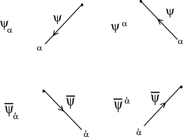
Figure 1: Weyl fermions.

Graphical Rule 1 ( Fig.1)
1. The arrow is pointed to the left for the chiral field $\psi$ and to the right for the anti-chiral one ${\bar{\psi}}$.(Complex structure)
2. The arrow is pointed to the up for the upper-suffix quantity and to the down for lower-suffix quantity.(Symplectic structure)
3. All spinor suffixes ($\alpha,\beta,\cdots$;${\dot{\alpha}},{\dot{\beta}},\cdots$) are labeled at the lowest position of arrow lines.

The choice of 3 is fixed by the condition that, when we express the basic SL(2,C)(Lorentz) invariants $\psi^{\alpha}\chi_{\alpha}$(NW-SE convention) =$\epsilon_{\alpha\beta}\psi^{\alpha}\psi^{\beta}$ , ${\bar{\psi}}_{\dot{\alpha}}{\bar{\chi}}^{\dot{\alpha}}$(SW-NE convention) =$\epsilon^{{\dot{\alpha}}{\dot{\beta}}}{\bar{\psi}}_{\dot{\alpha}}{\bar{\chi}}_{\dot{\beta}}$ where suffixes are contracted by the anti-symmetric tensor , the arrows continuously flow along the lines ( see Fig.4 which will be explained later) without changing the order of the spinor-field graphs.

Graphical Rule 2
Every spinor graph is anticommuting in the horizontal direction.

The derivatives of fermions are expressed as in Fig.2. We give it as a rule.

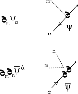
Figure 2: Derivatives of fermions.

Graphical Rule 3 ( Fig.2)
1. For each derivative, attach the derivative symbol "$\partial$" to the corresponding spinor-arrow with a dotted line as in Fig.2. At the end of the line, the Lorentz suffix of the derivative is described.
2. The order of the derivative lines described above is irrelevant because the derivative $\partial_{\mu}$ is commutative.

Following the above rule, the elements of the SL(2,C) $\sigma$-matrix are expressed as in Fig.3.

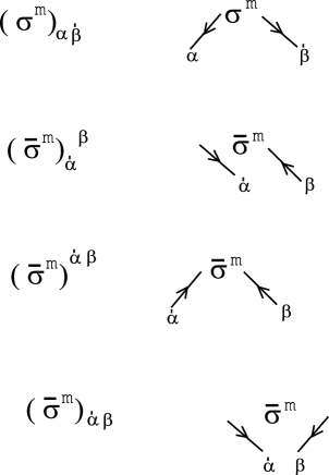
Figure 3: Elements of SL(2,C) $\sigma$-matrices. $(\sigma^{m})_{\alpha{\dot{\beta}}}$ and $({\bar{\sigma}}^{m})^{{\dot{\alpha}}\beta}$ are the standard form.

In Fig.3, the two arrows are directed ’horizontally outward’ for $\sigma$, whereas ’horizontally inward’ for ${\bar{\sigma}}$. We consider $(\sigma^{m})_{\alpha{\dot{\beta}}}$ and $({\bar{\sigma}}^{m})^{{\dot{\alpha}}\beta}$ are the standard form which is basically used in this text.

2.2 Spinor suffix contraction

Lorentz covariants and invariants are expressed by the contraction of the spinor suffixes. We take the convention of NW-SE contraction for the chiral suffix $\alpha$, and SW-NE contraction for the anti-chiral one ${\dot{\alpha}}$. They are expressed by connecting the corresponding suffix-ends as in Fig.4.

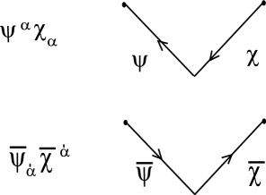
Figure 4: Contraction of spinor suffixes. [above] N(orth)W(est)-S(outh)E(ast) contraction for the chiral suffix $\alpha$ ($\psi^{\alpha}\chi_{\alpha}=\epsilon_{\alpha\beta}\psi^{\alpha}\psi^{\beta}$) : [below] SW-NE contraction for the anti-chiral suffix ${\dot{\alpha}}$ (${\bar{\psi}}_{\dot{\alpha}}{\bar{\chi}}^{\dot{\alpha}}=\epsilon^{{\dot{\alpha}}{\dot{\beta}}}{\bar{\psi}}_{\dot{\alpha}}{\bar{\chi}}_{\dot{\beta}}$).

The wedge structure, in Fig.4, characterizes all spinor contractions in the following. For the chiral-suffixes contraction, the wedge ’runs’ to the left, whereas the anti-chiral ones to the right.

Graphical Rule 4: Spinor Suffix Contraction ( Fig.4)
The contraction is expressed by connecting the corresponding suffix-ends.

Two Lorentz vectors, $\chi^{\alpha}(\sigma^{m})_{\alpha{\dot{\beta}}}{\bar{\psi}}^{\dot{\beta}}$ and ${\bar{\psi}}_{\dot{\alpha}}({\bar{\sigma}}^{m})^{{\dot{\alpha}}\beta}\chi_{\beta}$ are expressed as in Fig.5.

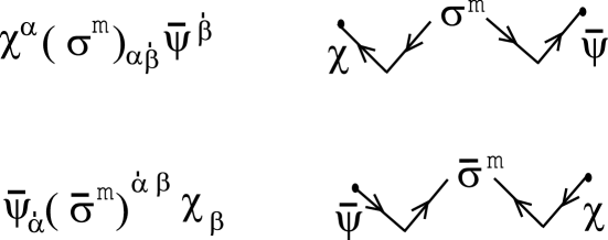
Figure 5: Two Lorentz vectors $\chi^{\alpha}(\sigma^{m})_{\alpha{\dot{\beta}}}{\bar{\psi}}^{\dot{\beta}}$ and ${\bar{\psi}}_{\dot{\alpha}}({\bar{\sigma}}^{m})^{{\dot{\alpha}}\beta}\chi_{\beta}$. The double wedge structure appears.

The double-wedge structure, in Fig.5, characterizes the vector quantities which involve one $\sigma^{m}$ or one ${\bar{\sigma}}^{m}$.

Next we take examples with two $\sigma$’s. $(\sigma^{n})_{\alpha{\dot{\alpha}}}({\bar{\sigma}}^{m})^{{\dot{\alpha}}\beta}$ and $({\bar{\sigma}}^{n})^{{\dot{\alpha}}\alpha}(\sigma^{m})_{\alpha{\dot{\beta}}}$ are expressed as in Fig.6.

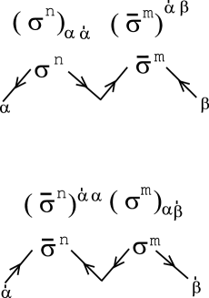
Figure 6: $(\sigma^{n})_{\alpha{\dot{\alpha}}}({\bar{\sigma}}^{m})^{{\dot{\alpha}}\beta}$ and $({\bar{\sigma}}^{n})^{{\dot{\alpha}}\alpha}(\sigma^{m})_{\alpha{\dot{\beta}}}$. The "spinor contraction" between $\sigma$ and ${\bar{\sigma}}$ is expressed as a wedge.

The "spinor contraction" between $\sigma$ and ${\bar{\sigma}}$ is also expressed as a wedge.

Graphical Rule 5: Space-Time Suffixes Contraction
The contraction of space-time suffix $m$ is expressed by a dotted line.

An example $\xi^{\alpha}(\sigma^{m})_{\alpha{\dot{\beta}}}\partial_{m}{\bar{\psi}}^{\dot{\beta}}$ is expressed as in Fig.7.

Figure 7: An Lorentz invariant: $\xi^{\alpha}(\sigma^{m})_{\alpha{\dot{\beta}}}\partial_{m}{\bar{\psi}}^{\dot{\beta}}$.

Note that
all dummy suffixes do not appear in the final invariant quantities.
The contraction is expressed by the directed wedges and the dotted curved lines. This makes the expression very transparent.

As the partially contracted examples, we take $({\bar{\sigma}}^{m})^{{\dot{\alpha}}\alpha}\xi_{\alpha}$ and $({\bar{\sigma}}^{m})_{\dot{\beta}}^{\leavevmode\nobreak\ \alpha}\xi_{\alpha}$. See Fig.8.

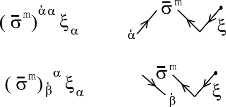
Figure 8: Partially contracted cases. $({\bar{\sigma}}^{m})^{{\dot{\alpha}}\alpha}\xi_{\alpha}$ and $({\bar{\sigma}}^{m})_{\dot{\beta}}^{\leavevmode\nobreak\ \alpha}\xi_{\alpha}$.

The spinor suffixes ${\dot{\alpha}},{\dot{\beta}}$ and the space-time suffix $m$ remain and wait for further contraction.

2.3 Graphical Formula

An important advantage of the graphical representation is the usage of graphical formulae (relations). It helps so much in practical calculation of SUSY quantities. Some demonstrations will be given later. We express the formula: $\psi^{\alpha}\chi_{\alpha}=-\psi_{\alpha}\chi^{\alpha}=\chi^{\alpha}\psi_{\alpha}$, ${\bar{\psi}}_{\dot{\alpha}}{\bar{\chi}}^{\dot{\alpha}}=-{\bar{\psi}}^{\dot{\alpha}}{\bar{\chi}}_{\dot{\alpha}}={\bar{\chi}}_{\dot{\alpha}}{\bar{\psi}}^{\dot{\alpha}}$ in Fig.9. The last equalities in the both lines of the figure comes from the anti-commutatibity of the spinor graphs(GR2).

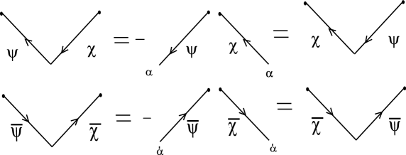
Figure 9: A graphical formula. $\psi^{\alpha}\chi_{\alpha}=-\psi_{\alpha}\chi^{\alpha}=\chi^{\alpha}\psi_{\alpha}$, and ${\bar{\psi}}_{\dot{\alpha}}{\bar{\chi}}^{\dot{\alpha}}=-{\bar{\psi}}^{\dot{\alpha}}{\bar{\chi}}_{\dot{\alpha}}={\bar{\chi}}_{\dot{\alpha}}{\bar{\psi}}^{\dot{\alpha}}$ .

We can express all formulae graphically. In this subsection, we list only basic ones. In Fig.10, the symmetric combination of ${\bar{\sigma}}^{m}\sigma^{n}$ are shown as the basic spinor algebra.

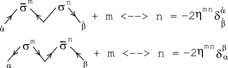
Figure 10: A graphical formula of the basic spinor algebra. $({\bar{\sigma}}^{m})^{{\dot{\alpha}}\beta}(\sigma^{n})_{\beta{\dot{\beta}}}+m\leftrightarrow n=-2\eta^{mn}\delta^{\dot{\alpha}}_{\dot{\beta}}$, and $(\sigma^{m})_{\alpha{\dot{\alpha}}}({\bar{\sigma}}^{n})^{{\dot{\alpha}}\beta}+m\leftrightarrow n=-2\eta^{mn}\delta^{\beta}_{\alpha}$.

The antisymmetric combination gives the generators of the Lorentz group, $\sigma^{nm},{\bar{\sigma}}^{nm}$.

$$(\sigma^{nm})_{\alpha}^{\leavevmode\nobreak\ \beta}=\frac{1}{4}\left\{\begin{array}[]{c}\mbox{ \includegraphics*[height=28.45274pt]{F1def2.eps} }\end{array}-m\leftrightarrow n\right\}{\quad,}$$ (3)

$$({\bar{\sigma}}^{nm})^{\dot{\alpha}}_{\leavevmode\nobreak\ {\dot{\beta}}}=\frac{1}{4}\left\{\begin{array}[]{c}\mbox{ \includegraphics*[height=28.45274pt]{F2def2.eps} }\end{array}-m\leftrightarrow n\right\}{\quad,}$$ (5)

Although we have already used ${\bar{\sigma}}^{m}$, its definition in terms of $\sigma^{m}$ and the "inverse" relation are displayed in Fig.11.

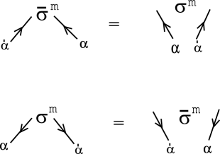
Figure 11: Definition of ${\bar{\sigma}}^{m}$, $({\bar{\sigma}}^{m})^{{\dot{\alpha}}\alpha}\equiv\epsilon^{{\alpha\beta}}\epsilon^{{\dot{\alpha}}{\dot{\beta}}}(\sigma^{m})_{\beta{\dot{\beta}}}=(\sigma^{m})^{\alpha{\dot{\alpha}}}$, and its "inverse" relation, $(\sigma^{m})_{\alpha{\dot{\alpha}}}=\epsilon_{{\dot{\alpha}}{\dot{\beta}}}\epsilon_{\alpha\beta}({\bar{\sigma}}^{m})^{{\dot{\beta}}\beta}=({\bar{\sigma}}^{m})_{{\dot{\alpha}}\alpha}$.

Here we do the upward and downward changes, within the $\sigma$ and ${\bar{\sigma}}$, by $\epsilon_{\alpha\beta}$ and $\epsilon^{\alpha\beta}$ as explained for the spinor in (1). Using the relation Fig.11, we can obtain the following useful relation.

Graphical Formula: Figure 11B

$$\begin{array}[]{c}\mbox{ \includegraphics*[height=28.45274pt]{F1vec3.eps} }\end{array}=\begin{array}[]{c}\mbox{ \includegraphics*[height=28.45274pt]{F2vec3.eps} }\end{array}$$ (8)

The "reduction" formulae (from the cubic $\sigma^{\prime}$s to the linear one) are expressed as in Fig.12.

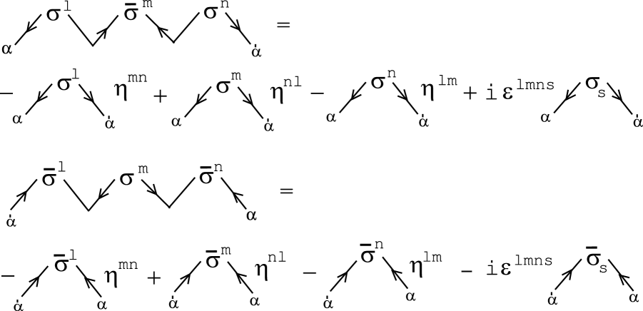
Figure 12: Two relations: 1) $\sigma^{l}{\bar{\sigma}}^{m}\sigma^{n}=-\sigma^{l}\eta^{mn}+\sigma^{m}\eta^{nl}-\sigma^{n}\eta^{lm}+i\epsilon^{lmns}\sigma_{s}$, 2) ${\bar{\sigma}}^{l}\sigma^{m}{\bar{\sigma}}^{n}=-{\bar{\sigma}}^{l}\eta^{mn}+{\bar{\sigma}}^{m}\eta^{nl}-{\bar{\sigma}}^{n}\eta^{lm}-i\epsilon^{lmns}{\bar{\sigma}}_{s}$.

From Fig.12, we notice any chain of $\sigma^{\prime}$s can always be expressed by less than three $\sigma^{\prime}$s. The appearance of the 4th rank anti-symmetric tensor $\epsilon^{abcd}$ is quite illuminating. The completeness relations are expressed as in Fig.13.

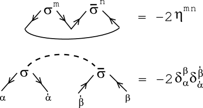
Figure 13: Completeness relations: 1) $\delta^{\alpha}_{\beta}(\sigma^{m})_{\alpha{\dot{\alpha}}}({\bar{\sigma}}^{n})^{{\dot{\alpha}}\beta}=-2\eta^{mn}$, 2) $(\sigma^{m})_{\alpha{\dot{\alpha}}}({\bar{\sigma}}_{m})^{{\dot{\beta}}\beta}=-2\delta^{\beta}_{\alpha}\delta^{\dot{\beta}}_{\dot{\alpha}}$. The contraction shown by a curve is the matrix trace. The relation 1) is also obtained from Fig.10.

The contraction, expressed by the directed curve in Fig.13, is the matrix trace. The Fierz identity is shown as.

$$\begin{array}[]{c}\mbox{ \includegraphics*[height=28.45274pt]{F1fierz.eps} }\end{array}=$$ (10)

$$\frac{1}{4}\left\{-\begin{array}[]{c}\mbox{ \includegraphics*[height=28.45274pt]{F2fierz.eps} }\end{array}\epsilon_{{\dot{\alpha}}{\dot{\beta}}}+\begin{array}[]{c}\mbox{ \includegraphics*[height=28.45274pt]{F3fierz.eps} }\end{array}\epsilon_{\alpha\beta}-m\leftrightarrow n\right\}$$ (13)

$$-{\frac{1}{2}}\eta^{nm}\epsilon_{\alpha\beta}\epsilon_{{\dot{\alpha}}{\dot{\beta}}}-\frac{1}{8}\left\{\begin{array}[]{c}\mbox{ \includegraphics*[height=28.45274pt]{F4fierz.eps} }\end{array}-l\leftrightarrow n\right\}\left\{\begin{array}[]{c}\mbox{ \includegraphics*[height=28.45274pt]{F5fierz.eps} }\end{array}-l\leftrightarrow m\right\},$$ (16)

where the relation: $(\sigma^{n})_{\alpha{\dot{\alpha}}}(\sigma^{m})_{\beta{\dot{\beta}}}=-\epsilon_{\beta\gamma}(\sigma^{nm})_{\alpha}^{\leavevmode\nobreak\ \gamma}\epsilon_{{\dot{\alpha}}{\dot{\beta}}}+\epsilon_{{\dot{\alpha}}{\dot{\gamma}}}({\bar{\sigma}}^{nm})^{\dot{\gamma}}_{\leavevmode\nobreak\ {\dot{\beta}}}\epsilon_{{\alpha\beta}}-{\frac{1}{2}}\eta^{nm}\epsilon_{\alpha\beta}\epsilon_{{\dot{\alpha}}{\dot{\beta}}}-2\epsilon_{\beta\gamma}(\sigma^{ln})_{\alpha}^{\leavevmode\nobreak\ \gamma}\epsilon_{{\dot{\alpha}}{\dot{\gamma}}}({\bar{\sigma}}_{l}^{\leavevmode\nobreak\ m})^{\dot{\gamma}}_{\leavevmode\nobreak\ {\dot{\beta}}}$, is expressed.

Finally we display 4$\sigma$’s cotraction formula.

$$\begin{array}[]{c}\mbox{ \includegraphics*[height=28.45274pt]{ssbssbBR.eps} }\end{array}=2(\eta^{lm}\eta^{ns}-\eta^{ln}\eta^{ms}+\eta^{ls}\eta^{mn}-i\epsilon^{lmns})$$ (18)

Its complex conjugate one is given by

$$\begin{array}[]{c}\mbox{ \includegraphics*[height=28.45274pt]{sbssbsR.eps} }\end{array}=2(\eta^{lm}\eta^{ns}-\eta^{ln}\eta^{ms}+\eta^{ls}\eta^{mn}+i\epsilon^{lmns})$$ (20)

The above 2 terms appear in the calculation of $W_{\alpha}W^{\alpha}$ and ${\bar{W}}_{\dot{\alpha}}{\bar{W}}^{\dot{\alpha}}$ respectively. ($W_{\alpha}$ and ${\bar{W}}_{\dot{\alpha}}$ are superfields of field strength. )

3 4D Chiral Multiplet

As the first example, we take the 4D chiral multiplet. It is made of a complex scalar field $A$, a Weyl spinor $\psi_{\alpha}$ and an auxiliary field (complex scalar) $F$. Their transformations are expressed as follows.

$$\delta_{\xi}A=\sqrt{2}\xi^{\alpha}\psi_{\alpha}=\sqrt{2}\begin{array}[]{c}\mbox{ \includegraphics*[height=28.45274pt]{F1chi1a.eps} }\end{array}{\quad,}$$ (22)

$$\delta_{\xi}\psi_{\alpha}=i\sqrt{2}{\sigma^{m}}_{\alpha{\dot{\alpha}}}{\bar{\xi}}^{\dot{\alpha}}\partial_{m}A+\sqrt{2}\xi_{\alpha}F=i\sqrt{2}\begin{array}[]{c}\mbox{ \includegraphics*[height=28.45274pt]{F2chi1a.eps} }\end{array}\partial_{m}A+\sqrt{2}\begin{array}[]{c}\mbox{ \includegraphics*[height=28.45274pt]{F3chi1a.eps} }\end{array}F{\quad,}$$ (25)

$$\delta_{\xi}F=i\sqrt{2}{\bar{\xi}}_{\dot{\alpha}}({\bar{\sigma}}^{m})^{{\dot{\alpha}}\beta}\partial_{m}\psi_{\beta}=i\sqrt{2}\begin{array}[]{c}\mbox{ \includegraphics*[height=28.45274pt]{F4chi1a.eps} }\end{array}{\quad.}$$ (27)

The complex conjugate ones are given as

$$\delta_{\xi}A^{*}=\sqrt{2}{\bar{\xi}}_{\dot{\alpha}}{\bar{\psi}}^{\dot{\alpha}}=\sqrt{2}\begin{array}[]{c}\mbox{ \includegraphics*[height=28.45274pt]{F1chi1b.eps} }\end{array}{\quad,}$$ (29)

$$\delta_{\xi}{\bar{\psi}}_{\dot{\alpha}}=i\sqrt{2}({{\bar{\sigma}}^{m}})^{\leavevmode\nobreak\ \alpha}_{\dot{\alpha}}\xi_{\alpha}\partial_{m}A^{*}+\sqrt{2}{\bar{\xi}}_{\dot{\alpha}}F^{*}=i\sqrt{2}\begin{array}[]{c}\mbox{ \includegraphics*[height=28.45274pt]{F2chi1bZr.eps} }\end{array}\partial_{m}A^{*}+\sqrt{2}\begin{array}[]{c}\mbox{ \includegraphics*[height=28.45274pt]{F3chi1b.eps} }\end{array}F^{*}{\quad,}$$ (32)

$$\delta_{\xi}F^{*}=i\sqrt{2}\xi^{\alpha}(\sigma^{m})_{\alpha{\dot{\beta}}}\partial_{m}{\bar{\psi}}^{\dot{\beta}}=i\sqrt{2}\begin{array}[]{c}\mbox{ \includegraphics*[height=28.45274pt]{F4chi1b.eps} }\end{array}{\quad.}$$ (34)

We can read the graphical rule of the complex conjugate operation by comparing (27) and (34).

Graphical Rule 6: Complex Conjugation Operation

$$\begin{array}[]{c}\mbox{ \includegraphics*[height=28.45274pt]{F1chi1a.eps} }\end{array}\quad\rightarrow\quad\begin{array}[]{c}\mbox{ \includegraphics*[height=28.45274pt]{F1chi1b.eps} }\end{array}{\quad,}$$ (37)

$$\begin{array}[]{c}\mbox{ \includegraphics*[height=28.45274pt]{F4chi1a.eps} }\end{array}\quad\rightarrow\quad-\begin{array}[]{c}\mbox{ \includegraphics*[height=28.45274pt]{F4chi1b.eps} }\end{array}{\quad.}$$ (40)

In order to show the graphical representation, presented in Sec.2, satisfies the SUSY representation and the usage of the graphical rules and formulae, we graphically show the SUSY symmetry of the Lagrangian.

$${\cal L}=i\partial_{n}{\bar{\psi}}_{\dot{\alpha}}({\bar{\sigma}}^{n})^{{\dot{\alpha}}\beta}\psi_{\beta}+A^{*}\Box A+F^{*}F{\quad,}$$

$$=\begin{array}[]{c}\mbox{ \includegraphics*[height=28.45274pt]{Fchi2.eps} }\end{array}+A^{*}\Box A+F^{*}F{\quad,}$$ (42)

(Hermiticity of the first term, up to a total derivative, can be confirmed by the use of GR6 anf Fig.11B.) The three terms in the Lagrangian transform as

$$\delta\left(i\begin{array}[]{c}\mbox{ \includegraphics*[height=28.45274pt]{F1chi3.eps} }\end{array}\right)=$$ (44)

$$i\begin{array}[]{c}\mbox{ \includegraphics*[height=28.45274pt]{F2chi3.eps} }\end{array}\left\{\begin{array}[]{c}i\sqrt{2}\begin{array}[]{c}\mbox{ \includegraphics*[height=28.45274pt]{F3chi3.eps} }\end{array}\partial_{m}A\\ <2>\end{array}+\begin{array}[]{c}\sqrt{2}\begin{array}[]{c}\mbox{ \includegraphics*[height=28.45274pt]{F4chi3.eps} }\end{array}F\\ <1>\end{array}\right\}$$ (52)

$$+i\partial_{n}\left\{\begin{array}[]{c}i\sqrt{2}\begin{array}[]{c}\mbox{ \includegraphics*[height=28.45274pt]{F5chi3.eps} }\end{array}\partial_{m}A^{*}\\ <4>\end{array}+\begin{array}[]{c}\sqrt{2}\begin{array}[]{c}\mbox{ \includegraphics*[height=28.45274pt]{F6chi3.eps} }\end{array}F^{*}\\ <3>\end{array}\right\}\begin{array}[]{c}\mbox{ \includegraphics*[height=28.45274pt]{F7chi3.eps} }\end{array}{\quad,}$$ (60)

$$\delta(A^{*}\Box A)=\begin{array}[]{c}\sqrt{2}\begin{array}[]{c}\mbox{ \includegraphics*[height=28.45274pt]{F8chi3.eps} }\end{array}\Box A\\ <2^{\prime}>\end{array}+\begin{array}[]{c}\sqrt{2}A^{*}\Box\left(\begin{array}[]{c}\mbox{ \includegraphics*[height=28.45274pt]{F9chi3.eps} }\end{array}\right)\\ <4^{\prime}>\end{array}{\quad,}$$ (67)

$$\delta(F^{*}F)=\begin{array}[]{c}i\sqrt{2}\begin{array}[]{c}\mbox{ \includegraphics*[height=28.45274pt]{F10chi3.eps} }\end{array}F\\ <1^{\prime}>\end{array}+\begin{array}[]{c}i\sqrt{2}F^{*}\begin{array}[]{c}\mbox{ \includegraphics*[height=28.45274pt]{F11chi3.eps} }\end{array}\\ <3^{\prime}>\end{array}{\quad.}$$ (74)

$<1>+<1^{\prime}>=0$ can be shown as

$$<1>=i\sqrt{2}\partial_{n}\left(\begin{array}[]{c}\mbox{ \includegraphics*[height=28.45274pt]{F12chi3.eps} }\end{array}\right)F$$ (76)

$$=i\sqrt{2}\partial_{n}\left(-\begin{array}[]{c}\mbox{ \includegraphics*[height=28.45274pt]{F13chi3.eps} }\end{array}\right)F=-<1^{\prime}>{\quad,}$$ (78)

where graph formula Fig.11B is used. $<2>+<2^{\prime}>=$ a total derivative is shown as

$$<2>=-\sqrt{2}\begin{array}[]{c}\mbox{ \includegraphics*[height=28.45274pt]{F14chi3.eps} }\end{array}\partial_{m}A=$$ (80)

$$-\sqrt{2}\partial_{n}\left(\begin{array}[]{c}\mbox{ \includegraphics*[height=28.45274pt]{F15chi3.eps} }\end{array}\partial_{m}A\right)$$ (82)

$$+\sqrt{2}\begin{array}[]{c}\mbox{ \includegraphics*[height=28.45274pt]{F15chi3.eps} }\end{array}\partial_{n}\partial_{m}A=$$ (84)

$$\mbox{ }\prime\prime\mbox{ }\quad\quad-\sqrt{2}\begin{array}[]{c}\mbox{ \includegraphics*[height=28.45274pt]{F8chi3.eps} }\end{array}\Box A=\mbox{ }\prime\prime\mbox{ }\quad\quad-<2^{\prime}>{\quad,}$$ (86)

where "$\mbox{ }\prime\prime\mbox{ }$" means the corresponding previous graph. In the above the relations Fig.10 and Fig.9 are used. $<4>+<4^{\prime}>=$ a total derivative can be shown as

$$<4>=-\sqrt{2}\begin{array}[]{c}\mbox{ \includegraphics*[height=28.45274pt]{F5chi3.eps} }\end{array}\partial_{n}\partial_{m}A\begin{array}[]{c}\mbox{ \includegraphics*[height=28.45274pt]{F7chi3.eps} }\end{array}$$ (89)

$$=\sqrt{2}\begin{array}[]{c}\mbox{ \includegraphics*[height=28.45274pt]{F17chi3.eps} }\end{array}\partial_{n}\partial_{m}A^{*}$$ (91)

$$=-\sqrt{2}\begin{array}[]{c}\mbox{ \includegraphics*[height=28.45274pt]{F9chi3.eps} }\end{array}\Box A^{*}{\quad,}$$ (93)

$$<4^{\prime}>=\partial_{n}\left\{\sqrt{2}A^{*}\partial^{n}(\begin{array}[]{c}\mbox{ \includegraphics*[height=28.45274pt]{F9chi3.eps} }\end{array})-\sqrt{2}\partial^{n}A^{*}\begin{array}[]{c}\mbox{ \includegraphics*[height=28.45274pt]{F9chi3.eps} }\end{array}\right\}$$ (96)

$$+\sqrt{2}\begin{array}[]{c}\mbox{ \includegraphics*[height=28.45274pt]{F9chi3.eps} }\end{array}\Box A^{*}{\quad,}$$ (98)

where some modification of Fig.11B is used in the first line, and Fig.10 is used in the second line. $<3>+<3^{\prime}>=$ a total derivative can be obtained as

$$<3>=i\sqrt{2}\partial_{n}\left(F^{*}\begin{array}[]{c}\mbox{ \includegraphics*[height=28.45274pt]{F18chi3.eps} }\end{array}\right)-i\sqrt{2}F^{*}\begin{array}[]{c}\mbox{ \includegraphics*[height=28.45274pt]{F11chi3.eps} }\end{array}$$ (101)

$$=\mbox{ }\prime\prime\mbox{ }\quad-<3^{\prime}>\ .$$ (102)

Summing the above results, we finally obtain the result without ignoring total drivatives.

$$\delta_{\xi}{\cal L}=\partial_{n}\left\{-\sqrt{2}\begin{array}[]{c}\mbox{ \includegraphics*[height=28.45274pt]{F15chi3.eps} }\end{array}\partial_{m}A+\sqrt{2}A^{*}\partial^{n}(\begin{array}[]{c}\mbox{ \includegraphics*[height=28.45274pt]{F9chi3.eps} }\end{array})\right.$$ (105)

$$\left.-\sqrt{2}\partial^{n}A^{*}\begin{array}[]{c}\mbox{ \includegraphics*[height=28.45274pt]{F9chi3.eps} }\end{array}+i\sqrt{2}F^{*}\begin{array}[]{c}\mbox{ \includegraphics*[height=28.45274pt]{F18chi3.eps} }\end{array}\right\}{\quad.}$$ (108)

Hence the Lagrangian indeed invariant up to a total derivative.

4 4D Vector Multiplet

The super elctromagnetic theory, in the WZ gauge, is given by

$${\cal L}_{EM}={\frac{1}{2}}D^{2}-\frac{1}{4}v^{mn}v_{mn}\begin{array}[]{c}\mbox{ \includegraphics*[height=28.45274pt]{vec1f.eps} }\end{array}{\quad,}$$ (110)

where $v_{mn}=\partial_{m}v_{n}-\partial_{n}v_{m}$. $v_{m}$ is the vector field, $\lambda$ is the Weyl fermion, $D$ is a scalar auxiliary field. (110) is invariant under the SUSY transformation.

$$\delta_{\xi}D=\begin{array}[]{c}\mbox{ \includegraphics*[height=28.45274pt]{D1vec2.eps} }\end{array}\begin{array}[]{c}\mbox{ \includegraphics*[height=28.45274pt]{D2vec2.eps} }\end{array}{\quad,}$$ (113)

$$\delta_{\xi}\begin{array}[]{c}\mbox{ \includegraphics*[height=28.45274pt]{L1vec2.eps} }\end{array}=\begin{array}[]{c}\mbox{ \includegraphics*[height=28.45274pt]{L2vec2.eps} }\end{array}D+\frac{1}{4}\left\{\begin{array}[]{c}\mbox{ \includegraphics*[height=28.45274pt]{L3vec2.eps} }\end{array}-m\leftrightarrow n\right\}v_{mn}{\quad,}$$ (117)

$$\delta_{\xi}v_{mn}=\begin{array}[]{c}\mbox{ \includegraphics*[height=28.45274pt]{F1vec2.eps} }\end{array}\begin{array}[]{c}\mbox{ \includegraphics*[height=28.45274pt]{F2vec2.eps} }\end{array}-m\leftrightarrow n{\quad,}$$ (120)

$$\delta_{\xi}v_{m}=\begin{array}[]{c}\mbox{ \includegraphics*[height=28.45274pt]{V1vec2.eps} }\end{array}\begin{array}[]{c}\mbox{ \includegraphics*[height=28.45274pt]{V2vec2.eps} }\end{array}{\quad,}$$ (123)

The SUSY invariance of (110) can be graphically shown by using the relations of Fig.9,Fig.11, Fig.12 and Fig.11B. The result is

$$\delta{\cal L}_{EM}=\partial_{l}\left[\begin{array}[]{c}\mbox{ \includegraphics*[height=28.45274pt]{F1vec4.eps} }\end{array}D\begin{array}[]{c}\mbox{ \includegraphics*[height=28.45274pt]{F2vec4.eps} }\end{array}v_{ml}\right.$$ (126)

$$\left.\begin{array}[]{c}\mbox{ \includegraphics*[height=28.45274pt]{F3vec4.eps} }\end{array}v_{mn}\right]{\quad,}$$ (128)

which expresses a total derivative. The appearance of the totally anti-symmetric tensor $\epsilon^{lmns}$ shows that the invariance crucially depends on the space-time dimensionality 4 in the case of vector multiplet. This fact makes the dimensional regularization difficult in the SUSY quantum calculation[8].

5 Majorana spinor

Another useful way to represent the supersymmetry is the use of the Majorana spinor which is based on SO(1,3) (not SL(2,C)) structure. We define the graphical representation for the Majorana spinor $\Psi$ and its conjugate ${\bar{\Psi}}=\Psi^{\dagger}\gamma_{0}$ as in Fig.14.

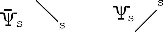
Figure 14: The graphical representation for the Majorana spinor, $\Psi$, and its conjugate ${\bar{\Psi}}=\Psi^{\dagger}\gamma_{0}$. $s=1,2,3,4.$

The SO(1,3) invariants ${\bar{\Psi}}\Psi$ and ${\bar{\Psi}}\gamma^{5}\Psi$ are represented as in Fig.15.

Figure 15: The graphical representation for the SO(1,3) invariants made of the Majorana spinors: ${\bar{\Psi}}\Psi$ and ${\bar{\Psi}}\gamma^{5}\Psi$.

They are graphically much simpler than the Weyl case ( no arrows, the single (vertical) wedge structure with spinor matrices placed at the vertex ) because only the adjoint structure is necessary to be build in the graph. Remaining information, such as hermiticity and chiral properties, is in the 4$\times$4 matrix elements (made of $\gamma^{m}$ matrices).

The relation between the Weyl and Majorana spinors is described in textbooks[9, 10, 11]. To show the precise relation, at the graphical level, and to show some usage of the graph method, we derive the relation using the previously defined contents. The chiral multiplet of Sec.3 is taken for the explanation.

First we introduce 4 real fields $P,Q,G,H$, instead of ($A,A^{*},F,F^{*}$).

$$P=\frac{1}{\sqrt{2}}(A+A^{*}){\quad,}\quad Q=\frac{1}{\sqrt{2}i}(A-A^{*}){\quad,}$$

$$G=\frac{1}{\sqrt{2}}(F+F^{*}){\quad,}\quad H=\frac{1}{\sqrt{2}i}(F-F^{*}){\quad.}$$ (129)

As for spinor quantities, we introduce 4 components spinor quantities $\alpha,{\bar{\alpha}},\Psi,{\bar{\Psi}}$ instead of the 2 components ones ($\xi,{\bar{\xi}},\psi,{\bar{\psi}}$).

$$\alpha=\left(\begin{array}[]{c}\xi_{\alpha}\\ {\bar{\xi}}^{\dot{\alpha}}\end{array}\right)\ {\quad,}\quad\Psi=\left(\begin{array}[]{c}\psi_{\alpha}\\ {\bar{\psi}}^{\dot{\alpha}}\end{array}\right)\ {\quad,}$$ (134)

$${\bar{\alpha}}=\left(\begin{array}[]{cc}\xi^{\alpha}&{\bar{\xi}}_{\dot{\alpha}}\end{array}\right){\quad,}\quad{\bar{\Psi}}=\left(\begin{array}[]{cc}\psi^{\alpha}&{\bar{\psi}}_{\dot{\alpha}}\end{array}\right){\quad.}$$ (137)

Using these quantities the SUSY transformation (of the chiral multiplet) is obtained as

$$\delta_{\xi}P=\xi^{\alpha}\psi_{\alpha}+{\bar{\xi}}_{\dot{\alpha}}{\bar{\psi}}^{\dot{\alpha}}={\bar{\alpha}}\Psi$$

$$=\begin{array}[]{c}\mbox{ \includegraphics*[height=28.45274pt]{F1majo3.eps} }\end{array}+\begin{array}[]{c}\mbox{ \includegraphics*[height=28.45274pt]{F2majo3.eps} }\end{array}=\begin{array}[]{c}\mbox{ \includegraphics*[height=28.45274pt]{F3majo3.eps} }\end{array}{\quad,}$$ (141)

$$\delta_{\xi}Q=\frac{1}{i}(\xi^{\alpha}\psi_{\alpha}-{\bar{\xi}}_{\dot{\alpha}}\psi^{\dot{\alpha}})={\bar{\alpha}}\gamma^{5}\Psi$$

$$=-i\begin{array}[]{c}\mbox{ \includegraphics*[height=28.45274pt]{F4majo3.eps} }\end{array}+i\begin{array}[]{c}\mbox{ \includegraphics*[height=28.45274pt]{F5majo3.eps} }\end{array}=\begin{array}[]{c}\mbox{ \includegraphics*[height=28.45274pt]{F6majo3.eps} }\end{array}{\quad,}$$ (145)

$$\delta_{\xi}G=i{\bar{\xi}}_{\dot{\alpha}}({\bar{\sigma}}^{m})^{{\dot{\alpha}}\beta}\partial_{m}\psi_{\beta}+i\xi^{\alpha}(\sigma^{m})_{\alpha{\dot{\beta}}}\partial_{m}{\bar{\psi}}^{\dot{\beta}}=i{\bar{\alpha}}\gamma^{m}\partial_{m}\Psi$$

$$=i\begin{array}[]{c}\mbox{ \includegraphics*[height=28.45274pt]{F7majo3.eps} }\end{array}+i\begin{array}[]{c}\mbox{ \includegraphics*[height=28.45274pt]{F8majo3.eps} }\end{array}=i\begin{array}[]{c}\mbox{ \includegraphics*[height=28.45274pt]{F9majo3.eps} }\end{array}{\quad,}$$ (149)

$$\delta_{\xi}H={\bar{\xi}}_{\dot{\alpha}}({\bar{\sigma}}^{m})^{{\dot{\alpha}}\beta}\partial_{m}\psi_{\beta}-\xi^{\alpha}(\sigma^{m})_{\alpha{\dot{\beta}}}\partial_{m}{\bar{\psi}}^{\dot{\beta}}=-i{\bar{\alpha}}\gamma^{5}\gamma^{m}\partial_{m}\Psi$$

$$=\begin{array}[]{c}\mbox{ \includegraphics*[height=28.45274pt]{F7majo3.eps} }\end{array}-\begin{array}[]{c}\mbox{ \includegraphics*[height=28.45274pt]{F8majo3.eps} }\end{array}=-i\begin{array}[]{c}\mbox{ \includegraphics*[height=28.45274pt]{F12majo3.eps} }\end{array}{\quad,}$$ (153)

$$\delta_{\xi}\Psi=\left(\begin{array}[]{c}\delta_{\xi}\psi_{\alpha}\\ \delta_{\xi}{\bar{\psi}}^{\dot{\alpha}}\end{array}\right)\ =\left(\begin{array}[]{c}i\sqrt{2}\begin{array}[]{c}\mbox{ \includegraphics*[height=28.45274pt]{F13majo3.eps} }\end{array}+\sqrt{2}\begin{array}[]{c}\mbox{ \includegraphics*[height=28.45274pt]{F14majo3.eps} }\end{array}F\\ i\sqrt{2}\begin{array}[]{c}\mbox{ \includegraphics*[height=28.45274pt]{F15majo3.eps} }\end{array}+\sqrt{2}\begin{array}[]{c}\mbox{ \includegraphics*[height=28.45274pt]{F16majo3.eps} }\end{array}F^{*}\end{array}\right)$$ (162)

$$=i\partial_{m}(P-\gamma^{5}Q)\gamma^{m}\alpha+(G-\gamma^{5}H)\alpha$$

$$=i\begin{array}[]{c}\mbox{ \includegraphics*[height=28.45274pt]{F17majo3.eps} }\end{array}+\begin{array}[]{c}\mbox{ \includegraphics*[height=28.45274pt]{F18majo3.eps} }\end{array}{\quad,}$$ (165)

where the double lines are used to express the SUSY parameters and the following gamma matrices are taken[6]:

$$\gamma^{m}=\left(\begin{array}[]{cc}0&(\sigma^{m})_{\alpha{\dot{\beta}}}\\ ({\bar{\sigma}}^{m})^{{\dot{\alpha}}\beta}&0\end{array}\right){\quad,}\quad\gamma^{5}=\gamma^{0}\gamma^{1}\gamma^{2}\gamma^{3}=\left(\begin{array}[]{cc}-i&0\\ 0&i\end{array}\right){\quad.}$$ (170)

We show, in (165), the graphical expressions for the SO(1,3) invariants made of the Majorana spinors: ${\bar{\alpha}}\Psi,{\bar{\alpha}}\gamma^{5}\Psi,i{\bar{\alpha}}\gamma^{m}\partial_{m}\Psi,-i{\bar{\alpha}}\gamma^{5}\gamma^{m}\partial_{m}\Psi,i\partial_{m}(P-\gamma^{5}Q)\gamma^{m}\alpha,(G-\gamma^{5}H)\alpha$. The above graphical relations manifestly show the $\gamma^{5}$ matrix controls the chirality in the Majorana spinor, whereas it is shown by the left-right direction (dot-undotted suffixes)in the Weyl case. The above relations can be used in the transformation between both expressions even at the graphical level.

The fermion kinetic term of the chiral Lagrangian (42) is graphically transformed into the Majorana expression as follows.

$$i\begin{array}[]{c}\mbox{ \includegraphics*[height=28.45274pt]{F1majo5.eps} }\end{array}=\frac{i}{2}\begin{array}[]{c}\mbox{ \includegraphics*[height=28.45274pt]{F1majo5.eps} }\end{array}-\frac{i}{2}\begin{array}[]{c}\mbox{ \includegraphics*[height=28.45274pt]{F2majo5.eps} }\end{array}$$ (174)

$$=\frac{i}{2}\partial_{m}\left(\begin{array}[]{c}\mbox{ \includegraphics*[height=28.45274pt]{F3majo5.eps} }\end{array}\right)-\frac{i}{2}\begin{array}[]{c}\mbox{ \includegraphics*[height=28.45274pt]{F4majo5.eps} }\end{array}-\frac{i}{2}\begin{array}[]{c}\mbox{ \includegraphics*[height=28.45274pt]{F2majo5.eps} }\end{array}$$ (178)

$$=\frac{i}{2}\partial_{m}(\mbox{ }\prime\prime\mbox{ })-\frac{i}{2}\left(\begin{array}[]{c}\psi_{\alpha}\\ {\bar{\psi}}^{\dot{\alpha}}\end{array}\right)\ \left(\begin{array}[]{cc}0&(\sigma^{m})_{\alpha{\dot{\beta}}}\\ ({\bar{\sigma}}^{m})^{{\dot{\alpha}}\beta}&0\end{array}\right)\partial_{m}\left(\begin{array}[]{cc}\psi^{\alpha}&{\bar{\psi}}_{\dot{\alpha}}\end{array}\right)$$ (184)

$$=\frac{i}{2}\partial_{m}(\mbox{ }\prime\prime\mbox{ })-\frac{i}{2}{\bar{\Psi}}\gamma^{m}\partial_{m}\Psi=\frac{i}{2}\partial_{m}(\mbox{ }\prime\prime\mbox{ })-\frac{i}{2}\begin{array}[]{c}\mbox{ \includegraphics*[height=28.45274pt]{F5majo5.eps} }\end{array}{\quad,}$$ (186)

where the relation of Fig.11B is used in the first line.

6 Indices of Graph

We introduce some indices of a graph. They classify graphs. Its use is another advantage of the graphical representation.

(i) Left Chiral Number and Right Chiral Number
We assign ${\frac{1}{2}}$ for each one step leftward arrow and define its total sum within a graph as Left Chiral Number(LCN). In the same way, we assign ${\frac{1}{2}}$ for each one step rightward arrow and define its total sum within a graph as Right Chiral Number(RCN).

(ii) Up-Down Counting
We assign $+{\frac{1}{2}}$ for one step of the upward arrow and $-{\frac{1}{2}}$ for the one step of the downward arrow. Then we define Left Up-Down Number(LUDN) as the total sum for all leftward arrows within a graph, and Right Up-Down Number(RUDN) as the total sum for all rightward arrows within a graph. For SL(2,C) invariants, these indices vanish.

In order to count the number of the suffix contraction we introduce the following ones.

(iii) Left Wedge Number and Right Wedge Number
We assign $1$ for each piece of $\begin{array}[]{c}\mbox{ \includegraphics*[height=28.45274pt]{Lwedge.eps} }\end{array}$ and define the total sum within a graph as Left Wedge Number(LWN). In the same way, we assign $1$ for each piece of $\begin{array}[]{c}\mbox{ \includegraphics*[height=28.45274pt]{Rwedge.eps} }\end{array}$ and define the total sum within a graph as Right Wedge Number(RWN).

(iv) Dotted Line Number
We assign $1$ for one dotted line which shows a space-time suffix contraction. We define the total sum within a graph as Dotted Line Number(DLN).

In addition to the graph-related indices, we introduce
a) Physical Dimension (DIM); b) Number of the differentials (DIF); c) Number of $\sigma$ or ${\bar{\sigma}}$ (SIG)

We list the above indices for basic spinor quantities in Table 1 and for the operators appearing the chiral multiplet Lagrangian (Sec.3) in Table 2.

	$\begin{array}[]{c}\mbox{ \includegraphics*[height=28.45274pt]{F1t1.eps} }\end{array}$	$\begin{array}[]{c}\mbox{ \includegraphics*[height=28.45274pt]{F2t1.eps} }\end{array}$	$\begin{array}[]{c}\mbox{ \includegraphics*[height=28.45274pt]{F3t1.eps} }\end{array}$	$\begin{array}[]{c}\mbox{ \includegraphics*[height=28.45274pt]{F4t1.eps} }\end{array}$
(LCN, RCN)	$({\frac{1}{2}},0)$	$(0,{\frac{1}{2}})$	$({\frac{1}{2}},{\frac{1}{2}})$	$({\frac{1}{2}},{\frac{1}{2}})$
(LUDN, RUDN)	$(-{\frac{1}{2}},0)$	$(0,+{\frac{1}{2}})$	$(-{\frac{1}{2}},-{\frac{1}{2}})$	$({\frac{1}{2}},{\frac{1}{2}})$
(LWN, RWN)	0	0	0	0
DLN	0	0	0	0
DIM	$\frac{3}{2}$	$\frac{3}{2}$	0	0
DIF	0	0	0	0
SIG	0	0	1	1
Table 1  Indices for basic spinor quantities: $\psi_{\alpha},{\bar{\psi}}^{\dot{\alpha}},(\sigma^{m})_{\alpha{\dot{\beta}}}$ and $({\bar{\sigma}}^{m})^{{\dot{\alpha}}\beta}$.

	$\begin{array}[]{c}\mbox{ \includegraphics*[height=28.45274pt]{Fchi2.eps} }\end{array}$	$A^{*}\Box A$	$F^{*}F$
(LCN, RCN)	$(1,1)$	/	/
(LUDN, RUDN)	$(0,0)$	/	/
(LWN, RWD)	(1,1)	/	/
DLN	1	/	/
DIM	$4$	$4$	$4$
DIF	$1$	$2$	$0$
SIG	$1$	$0$	$0$
Table 2 Indices for operators appearing in the chiral multiplet Lagrangian.

We can identify every term appearing in the theory in terms of some of these indices. We list some indices for all spinorial operators in Super QED. We see all terms are classified by the indices and the field contents.

		(LCN,RCN)
		=(LWN,RWN)	(LUDN,RUDN)	DIF	Fields
1	$-i\begin{array}[]{c}\mbox{ \includegraphics*[height=28.45274pt]{F1t3.eps} }\end{array}$	$(1,1)$	$(0,0)$	$1$	$\lambda,{\bar{\lambda}}$
2	$i\begin{array}[]{c}\mbox{ \includegraphics*[height=28.45274pt]{F2t3.eps} }\end{array}$	$(1,1)$	$(0,0)$	$1$	$\psi_{+},{\bar{\psi}}_{+}$
3	$i\begin{array}[]{c}\mbox{ \includegraphics*[height=28.45274pt]{F3t3.eps} }\end{array}$	$(1,1)$	$(0,0)$	$1$	$\psi_{-},{\bar{\psi}}_{-}$
4	$\frac{e}{2}\begin{array}[]{c}\mbox{ \includegraphics*[height=28.45274pt]{F4t3.eps} }\end{array}$	$(1,1)$	$(0,0)$	$0$	$\psi_{+},{\bar{\psi}}_{+},v^{m}$
5	$-\frac{e}{2}\begin{array}[]{c}\mbox{ \includegraphics*[height=28.45274pt]{F5t3.eps} }\end{array}$	$(1,1)$	$(0,0)$	$0$	$\psi_{-},{\bar{\psi}}_{-},v^{m}$
6	$-\frac{ie}{\sqrt{2}}A_{+}\begin{array}[]{c}\mbox{ \includegraphics*[height=28.45274pt]{F6t3.eps} }\end{array}$	$(0,1)$	$(0,0)$	$0$	$A_{+},{\bar{\psi}}_{+},{\bar{\lambda}}$
7	$+\frac{ie}{\sqrt{2}}A_{-}\begin{array}[]{c}\mbox{ \includegraphics*[height=28.45274pt]{F7t3.eps} }\end{array}$	$(0,1)$	$(0,0)$	$0$	$A_{-},{\bar{\psi}}_{-},{\bar{\lambda}}$
8	$+\frac{ie}{\sqrt{2}}A_{+}^{*}\begin{array}[]{c}\mbox{ \includegraphics*[height=28.45274pt]{F8t3.eps} }\end{array}$	$(1,0)$	$(0,0)$	$0$	$A^{*}_{+},\psi_{+},\lambda$
9	$-\frac{ie}{\sqrt{2}}A_{-}^{*}\begin{array}[]{c}\mbox{ \includegraphics*[height=28.45274pt]{F9t3.eps} }\end{array}$	$(1,0)$	$(0,0)$	$0$	$A^{*}_{-},\psi_{-},\lambda$
10	$-m\begin{array}[]{c}\mbox{ \includegraphics*[height=28.45274pt]{F10t3.eps} }\end{array}$	$(1,0)$	$(0,0)$	$0$	$\psi_{+},\psi_{-}$
11	$-m\begin{array}[]{c}\mbox{ \includegraphics*[height=28.45274pt]{F11t3.eps} }\end{array}$	$(0,1)$	$(0,0)$	$0$	${\bar{\psi}}_{+},{\bar{\psi}}_{-}$
Table 3  List of indices for all spinor operators in the super QED Lagrangian.
$(\lambda,{\bar{\lambda}})$: photino; $v^{m}$: photon; $(\psi_{+},{\bar{\psi}}_{+})$: $+e$ chiral fermion; $(\psi_{-},{\bar{\psi}}_{-})$: $-e$ chiral fermion.

The product of $\sigma$-matrices appear in the intermediate stage of SUSY calculation. Its classification is an important subject because that fixes the right (graphical) formula to be used for reduction of SUSY quantities. We list the result, by using the graph indices defined in this section, in TABLE 4, 5, 6 for the case of 2$\sigma$’s, 3$\sigma$’s and 4$\sigma$’s respectively. This result is exploited in the C-program calculation of SUSY[7].

DLN	LWN	RWN	figure
	0	0	$\begin{array}[]{c}\mbox{ \includegraphics*[height=28.45274pt]{sig2Ar.eps} }\end{array}$
0	0	1	$\begin{array}[]{c}\mbox{ \includegraphics*[height=28.45274pt]{sig2Cr.eps} }\end{array}$
	1	0	$\begin{array}[]{c}\mbox{ \includegraphics*[height=28.45274pt]{sig2Cbr.eps} }\end{array}$
	1	1	$\begin{array}[]{c}\mbox{ \includegraphics*[height=28.45274pt]{sig2Dr.eps} }\end{array}\ =-2\eta^{mn}$
	0	0	$\begin{array}[]{c}\mbox{ \includegraphics*[height=28.45274pt]{sig2Br.eps} }\end{array}\ =-2\epsilon_{\alpha\beta}\epsilon_{{\dot{\alpha}}{\dot{\beta}}}$
1	0	1	$\begin{array}[]{c}\mbox{ \includegraphics*[height=28.45274pt]{sig2Fr.eps} }\end{array}\ =-4\delta^{\beta}_{\alpha}$
	1	0	$\begin{array}[]{c}\mbox{ \includegraphics*[height=28.45274pt]{sig2Fbr.eps} }\end{array}\ =-4\delta_{\dot{\beta}}^{\dot{\alpha}}$
	1	1	$\begin{array}[]{c}\mbox{ \includegraphics*[height=28.45274pt]{sig2Er.eps} }\end{array}\ =-8$
TABLE 4 Classification of the product of 2 sigma matrices (nsi=2).

DLN	LWN	RWN	figure
	0	0	$\begin{array}[]{c}\mbox{ \includegraphics*[height=28.45274pt]{sig3Ar.eps} }\end{array}$
0	0	1	$\begin{array}[]{c}\mbox{ \includegraphics*[height=28.45274pt]{sig3Cbr.eps} }\end{array}$
	1	0	$\begin{array}[]{c}\mbox{ \includegraphics*[height=28.45274pt]{sig3Cr.eps} }\end{array}$
	1	1	closed-chiral-loop No =1 $\begin{array}[]{c}\mbox{ \includegraphics*[height=28.45274pt]{sig3Er.eps} }\end{array}$
			closed-chiral-loop No =0 $\begin{array}[]{c}\mbox{ \includegraphics*[height=28.45274pt]{sig3Gr.eps} }\end{array}$
	0	0	$-2\epsilon_{\alpha\beta}\epsilon_{{\dot{\alpha}}{\dot{\beta}}}\ \begin{array}[]{c}\mbox{ \includegraphics*[height=28.45274pt]{sig3Br.eps} }\end{array}$
1	0	1	$-4\delta^{\beta}_{\alpha}\ \begin{array}[]{c}\mbox{ \includegraphics*[height=28.45274pt]{sig3Dr.eps} }\end{array}$
	1	0	$-4\delta^{\dot{\alpha}}_{\dot{\beta}}\ \begin{array}[]{c}\mbox{ \includegraphics*[height=28.45274pt]{sig3Dr.eps} }\end{array}$
	1	1	$-8\ \begin{array}[]{c}\mbox{ \includegraphics*[height=28.45274pt]{sig3Fr.eps} }\end{array}$
TABLE 5 Classification of the product of 3 sigma matrices (nsi=3).

DLN	LWN	RWN	figure
	0	0	$\begin{array}[]{c}\mbox{ \includegraphics*[height=28.45274pt]{sig4Ar.eps} }\end{array}$
	0	1	$\begin{array}[]{c}\mbox{ \includegraphics*[height=28.45274pt]{sig4Br.eps} }\end{array}$
	1	0	$\begin{array}[]{c}\mbox{ \includegraphics*[height=28.45274pt]{sig4Cr.eps} }\end{array}$
			GrNum=2, Division=(2,2) $\begin{array}[]{c}\mbox{ \includegraphics*[height=28.45274pt]{sig4Dr.eps} }\end{array}$
	1	1	GrNum=2, Division=(3,1) $\begin{array}[]{c}\mbox{ \includegraphics*[height=28.45274pt]{sig4Er.eps} }\end{array}$
			GrNum=3, Division=(2,1,1) $\begin{array}[]{c}\mbox{ \includegraphics*[height=28.45274pt]{sig4Fr.eps} }\end{array}$
0	2	0	$\begin{array}[]{c}\mbox{ \includegraphics*[height=28.45274pt]{sig4Gr.eps} }\end{array}$
	0	2	$\begin{array}[]{c}\mbox{ \includegraphics*[height=28.45274pt]{sig4Hr.eps} }\end{array}$
	1	2	GrNum=1, $\begin{array}[]{c}\mbox{ \includegraphics*[height=28.45274pt]{sig4Ir.eps} }\end{array}$
			GrNum=2, $\begin{array}[]{c}\mbox{ \includegraphics*[height=28.45274pt]{sig4Jr.eps} }\end{array}$
	2	1	GrNum=1, $\begin{array}[]{c}\mbox{ \includegraphics*[height=28.45274pt]{sig4Kr.eps} }\end{array}$
			GrNum=2, $\begin{array}[]{c}\mbox{ \includegraphics*[height=28.45274pt]{sig4Lr.eps} }\end{array}$
	2	2	GrNum=1, $\begin{array}[]{c}\mbox{ \includegraphics*[height=28.45274pt]{ssbssbBR.eps} }\end{array}$
			GrNum=2, $\begin{array}[]{c}\mbox{ \includegraphics*[height=28.45274pt]{sig4Mr.eps} }\end{array}$
TABLE 6 Classification of the product of 4 sigma matrices with
no vector-suffix contraction (nsi=4, DLN=0).

7 Superspace Quantities

We know the SUSY symmetry is most naturally viewed in the superspace ($x^{m},\theta,{\bar{\theta}}$). Here we introduce anti-commuting parameters $\theta_{\alpha}=\epsilon_{\alpha\beta}\theta^{\beta},\theta^{\alpha},{\bar{\theta}}_{\dot{\alpha}},{\bar{\theta}}^{\dot{\alpha}}=\epsilon^{{\dot{\alpha}}{\dot{\beta}}}{\bar{\theta}}_{\dot{\beta}}$ as the basic spinor coordinate. We show them graphically in Fig.16.

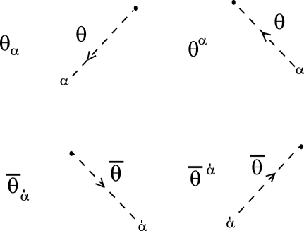
Figure 16: The graphical representation for the spinor coordinates in the superspace: $\theta_{\alpha},\theta^{\alpha},{\bar{\theta}}_{\dot{\alpha}}$ and ${\bar{\theta}}^{\dot{\alpha}}$.

They satisfy the graphical relations of Fig.17.

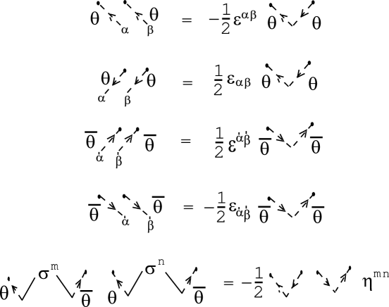
Figure 17: The graphical rules for the spinor coordinates: $\theta^{\alpha}\theta^{\beta}=-{\frac{1}{2}}\epsilon^{\alpha\beta}\theta\theta,\leavevmode\nobreak\ \theta_{\alpha}\theta_{\beta}={\frac{1}{2}}\epsilon_{\alpha\beta}\theta\theta,\leavevmode\nobreak\ {\bar{\theta}}^{\dot{\alpha}}{\bar{\theta}}^{\dot{\beta}}={\frac{1}{2}}\epsilon^{{\dot{\alpha}}{\dot{\beta}}}{\bar{\theta}}{\bar{\theta}},\leavevmode\nobreak\ {\bar{\theta}}_{\dot{\alpha}}{\bar{\theta}}_{\dot{\beta}}=-{\frac{1}{2}}\epsilon_{{\dot{\alpha}}{\dot{\beta}}}{\bar{\theta}}{\bar{\theta}},\leavevmode\nobreak\ \theta\sigma^{m}{\bar{\theta}}\theta\sigma^{n}{\bar{\theta}}=-{\frac{1}{2}}\theta\theta{\bar{\theta}}{\bar{\theta}}\eta^{mn}$.

The general superfield $F(x,\theta,{\bar{\theta}})$, in terms of components fields
($f(x),\phi(x),{\bar{\chi}}(x),m(x),n(x),v_{m}(x),{\bar{\lambda}}(x),\psi(x),d(x)$) , is shown as

$$F(x,\theta,{\bar{\theta}})=$$

$$f(x)+\begin{array}[]{c}\mbox{ \includegraphics*[height=28.45274pt]{F1ss1.eps} }\end{array}+\begin{array}[]{c}\mbox{ \includegraphics*[height=28.45274pt]{F2ss1.eps} }\end{array}+\begin{array}[]{c}\mbox{ \includegraphics*[height=28.45274pt]{F3ss1.eps} }\end{array}m(x)+\begin{array}[]{c}\mbox{ \includegraphics*[height=28.45274pt]{F4ss1.eps} }\end{array}n(x)$$ (191)

$$+\begin{array}[]{c}\mbox{ \includegraphics*[height=28.45274pt]{F5ss1.eps} }\end{array}v_{m}(x)+\begin{array}[]{c}\mbox{ \includegraphics*[height=28.45274pt]{F6ss1.eps} }\end{array}+\begin{array}[]{c}\mbox{ \includegraphics*[height=28.45274pt]{F7ss1.eps} }\end{array}$$ (195)

$$+\begin{array}[]{c}\mbox{ \includegraphics*[height=28.45274pt]{F8ss1.eps} }\end{array}d(x){\quad.}$$ (197)

The SUSY transformation generator $Q_{\alpha}$ and ${\bar{Q}}^{\dot{\alpha}}$ are expressed as

$$Q_{\alpha}=\frac{\partial}{\partial\theta^{\alpha}}-i\begin{array}[]{c}\mbox{ \includegraphics*[height=28.45274pt]{F1ss2.eps} }\end{array}{\quad,}$$ (199)

$${\bar{Q}}^{\dot{\alpha}}=\frac{\partial}{\partial{\bar{\theta}}_{\dot{\alpha}}}+i\begin{array}[]{c}\mbox{ \includegraphics*[height=28.45274pt]{F2ss2.eps} }\end{array}{\quad,}$$ (201)

The SUSY derivative operators $D$ and ${\bar{D}}$, which are the conjugate partners of $Q$ and ${\bar{Q}}$, are expressed as

$$D_{\alpha}=\frac{\partial}{\partial\theta^{\alpha}}+i\begin{array}[]{c}\mbox{ \includegraphics*[height=28.45274pt]{F1ss2.eps} }\end{array}{\quad,}$$ (203)

$${\bar{D}}_{\dot{\alpha}}=-\frac{\partial}{\partial{\bar{\theta}}^{\dot{\alpha}}}-i\begin{array}[]{c}\mbox{ \includegraphics*[height=28.45274pt]{F2ss3.eps} }\end{array}{\quad,}$$ (205)

We can graphically confirm the SUSY algebra by using the commutativity and anti-commutativity between $\theta,{\bar{\theta}},\frac{\partial}{\partial\theta},\frac{\partial}{\partial{\bar{\theta}}}$ and $\partial_{m}$.

$$\{Q_{\alpha},{\bar{Q}}_{\dot{\alpha}}\}=2i\begin{array}[]{c}\mbox{ \includegraphics*[height=28.45274pt]{F1ss4.eps} }\end{array}{\quad,}$$ (207)

$$\{D_{\alpha},{\bar{D}}_{\dot{\alpha}}\}=-2i\begin{array}[]{c}\mbox{ \includegraphics*[height=28.45274pt]{F1ss4.eps} }\end{array}{\quad.}$$ (209)

In the treatment of the chiral superfield, it is important to choose appropriate coordinates: ($y^{m}=x^{m}+i\theta\sigma^{m}{\bar{\theta}},\theta,{\bar{\theta}}$) for the chiral field, and ($y^{{\dagger}m}=x^{m}-i\theta\sigma^{m}{\bar{\theta}},\theta,{\bar{\theta}}$) for the anti-chiral one.

$$y^{m}=x^{m}+i\begin{array}[]{c}\mbox{ \includegraphics*[height=28.45274pt]{F1ss5.eps} }\end{array}{\quad,}$$ (211)

$$y^{{\dagger}m}=x^{m}-i\begin{array}[]{c}\mbox{ \includegraphics*[height=28.45274pt]{F1ss5.eps} }\end{array}{\quad.}$$ (213)

Because of the properties (${\bar{D}}_{\dot{\alpha}}y^{m}=0,{\bar{D}}_{\dot{\alpha}}\theta=0$) and ($D_{\alpha}y^{{\dagger}m}=0,D_{\alpha}{\bar{\theta}}=0$), the chiral superfield $\Phi$ (${\bar{D}}_{\dot{\alpha}}\Phi=0$) and the anti-chiral one $\Phi^{\dagger}$ ($D_{\alpha}\Phi^{\dagger}=0$) are always written as

$$\Phi(y,\theta,{\bar{\theta}})=A(y)+\sqrt{2}\begin{array}[]{c}\mbox{ \includegraphics*[height=28.45274pt]{F1ss6.eps} }\end{array}+\begin{array}[]{c}\mbox{ \includegraphics*[height=28.45274pt]{F3ss1.eps} }\end{array}F(y){\quad,}$$ (216)

and

$$\Phi^{\dagger}(y^{\dagger},\theta,{\bar{\theta}})=A^{*}(y^{\dagger})+\sqrt{2}\begin{array}[]{c}\mbox{ \includegraphics*[height=28.45274pt]{F2ss6.eps} }\end{array}+\begin{array}[]{c}\mbox{ \includegraphics*[height=28.45274pt]{F4ss1.eps} }\end{array}F^{*}(y^{\dagger}){\quad,}$$ (219)

respectively. The SUSY differential operators are expressed as, in terms of ($y,\theta,{\bar{\theta}}$),

$$D_{\alpha}=\frac{\partial}{\partial\theta^{\alpha}}+2i\begin{array}[]{c}\mbox{ \includegraphics*[height=28.45274pt]{F1ss7.eps} }\end{array}{\quad,}\quad{\bar{D}}_{\dot{\alpha}}=-\frac{\partial}{\partial{\bar{\theta}}^{\dot{\alpha}}}{\quad,}$$ (221)

$$Q_{\alpha}=\frac{\partial}{\partial\theta^{\alpha}}{\quad,}\quad{\bar{Q}}_{\dot{\alpha}}=-\frac{\partial}{\partial{\bar{\theta}}^{\dot{\alpha}}}+2i\begin{array}[]{c}\mbox{ \includegraphics*[height=28.45274pt]{F2ss7.eps} }\end{array}{\quad.}$$ (223)

and as, in terms of ($y^{\dagger},\theta,{\bar{\theta}}$),

$$D_{\alpha}=\frac{\partial}{\partial\theta^{\alpha}}{\quad,}\quad{\bar{D}}_{\dot{\alpha}}=-\frac{\partial}{\partial{\bar{\theta}}^{\dot{\alpha}}}-2i\begin{array}[]{c}\mbox{ \includegraphics*[height=28.45274pt]{F1ss8.eps} }\end{array}{\quad,}$$ (225)

$$Q_{\alpha}=\frac{\partial}{\partial\theta^{\alpha}}-2i\begin{array}[]{c}\mbox{ \includegraphics*[height=28.45274pt]{F2ss8.eps} }\end{array}{\quad,}\quad{\bar{Q}}_{\dot{\alpha}}=-\frac{\partial}{\partial{\bar{\theta}}^{\dot{\alpha}}}{\quad.}$$ (227)

The superspace calculation can be performed graphically. For example, the $\Phi^{\dagger}\Phi$ calculation, in order to find the 4D SUSY Lagragian, can be done using the graph relations of Fig.17. An advantage, compared to the usual one, is that the graphically expressed quantity is not "obscured" by the dummy (contracted) suffixes.

8 Application to 5D Supersymmetry

In this section we apply the graphical method to a recent subject [12, 13]: 5D supersymmetry. Here both (4-components and 2-components spinors) types of representation appear in relation to SUSY "decomposition". Stimulated by the brane world physics, higher dimensional SUSY becomes an important subject. In particular, 5 dimensional one is used as a concrete extended model of the standard model. The simplest one is the hypermultiplet $(A^{i},\chi,F_{i})$, where both $A^{i}$($i=1,2$) and $F^{i}$ are the SU(2)_R doublet of complex scalars. $F^{i}$ are the auxiliary fields. $\chi$ is a Dirac field. The SU(2)_R suffix, $i$, is lowered or raised by $\epsilon_{ij}$ and $\epsilon^{ij}$: $A_{i}=\epsilon_{ij}A^{j},F^{i}=\epsilon^{ij}F_{j}$ where $\epsilon_{ij}$ and $\epsilon^{ij}$ are the same as (1).

The doublet fields are graphically represented as in Fig.18.

Figure 18: The graphical representation for the SU(2)_R doublet fields, $A^{i},A_{i}=\epsilon_{ij}A^{j},F_{i}$ and $F^{i}=\epsilon^{ij}F_{j}$. The arrowed dotted line is depicted arbitrarily as far as the one end is attached to the symbol and the correct arrow direction is taken.

The SU(2)_R suffix up-down is expressed by the arrow direction: the flow-in direction for the up-suffix and the flow-out direction for the down-suffix. (This representation of the suffix up-down is different from the treatment taken in the spinor-suffix case of Sec.2.)

As the 5D SUSY parameter, we take the symplectic Majorana spinors. They are SU(2)_R doublet of Dirac spinors $\xi^{i}$($i=1,2$) which satisfy the symplectic Majorana condition ("reality" condition).

$$\xi^{i}=\epsilon^{ij}C{\bar{\xi}}_{j}^{T}{\quad,}\quad C=\left(\begin{array}[]{cc}i\sigma^{2}&0\\ 0&i\sigma^{2}\end{array}\right){\quad.}$$ (230)

From the number of the independent SUSY parameters, we know the present system has 8 (counted in real) supercharges. We introduce the graphical representation for $\xi^{i}$ and ${\bar{\xi}}_{i}$ as in Fig.19. The Dirac spinor structure is graphically the same as the Majorana one of Sec.5.

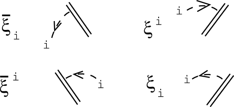
Figure 19: The graphical representation for the 5D SUSY parameters, ${\bar{\xi}}_{i},\xi^{i},{\bar{\xi}}^{i}$ and $\xi_{i}$.

Then the 5D SUSY transformation is expressed as

$$\delta_{\xi}A^{i}=-\sqrt{2}\epsilon^{ij}{\bar{\xi}}_{j}\chi=-\sqrt{2}\begin{array}[]{c}\mbox{ \includegraphics*[height=28.45274pt]{F1fds2.eps} }\end{array}{\quad,}$$ (232)

$$\delta_{\xi}\chi=\sqrt{2}i\gamma^{M}\partial_{M}A^{i}\epsilon_{ij}\xi^{j}+\sqrt{2}F_{i}\xi^{i}$$

$$=\sqrt{2}i\begin{array}[]{c}\mbox{ \includegraphics*[height=28.45274pt]{F2fds2.eps} }\end{array}+\sqrt{2}\begin{array}[]{c}\mbox{ \includegraphics*[height=28.45274pt]{F3fds2.eps} }\end{array}{\quad,}$$ (235)

$$\delta_{\xi}F_{i}=\sqrt{2}i{\bar{\xi}}_{i}\gamma^{M}\partial_{M}\chi=\sqrt{2}i\begin{array}[]{c}\mbox{ \includegraphics*[height=28.45274pt]{F4fds2.eps} }\end{array}{\quad,}$$ (237)

where a wavy line is used to express the contraction of the 5D space-time suffixes ($M=0,1,2,3,5$). The complex conjugate one is given by

$$\delta_{\xi}A^{*}_{i}=\sqrt{2}\epsilon_{ij}{\bar{\chi}}\xi^{j}=\sqrt{2}\begin{array}[]{c}\mbox{ \includegraphics*[height=28.45274pt]{F1fds3.eps} }\end{array}{\quad,}$$ (239)

$$\delta_{\xi}{\bar{\chi}}=-\sqrt{2}i{\bar{\xi}}_{i}\gamma^{M}\partial_{M}A^{*}_{j}\epsilon^{ij}+\sqrt{2}{\bar{\xi}}_{i}F^{*i}$$

$$=-\sqrt{2}i\begin{array}[]{c}\mbox{ \includegraphics*[height=28.45274pt]{F2fds3.eps} }\end{array}+\sqrt{2}\begin{array}[]{c}\mbox{ \includegraphics*[height=28.45274pt]{F3fds3.eps} }\end{array}{\quad,}$$ (242)

$$\delta_{\xi}F^{*i}=-\sqrt{2}i\partial_{M}{\bar{\chi}}\gamma^{M}\xi^{i}=-\sqrt{2}i\begin{array}[]{c}\mbox{ \includegraphics*[height=28.45274pt]{F4fds3.eps} }\end{array}{\quad,}$$ (244)

The free Lagrangian is given by

$${\cal L}=-i{\bar{\chi}}\gamma^{M}\partial_{M}\chi-\partial^{M}A^{*}_{i}\partial_{M}A^{i}+F^{*i}F_{i}$$

$$=-i\begin{array}[]{c}\mbox{ \includegraphics*[height=28.45274pt]{F1fds4.eps} }\end{array}-\begin{array}[]{c}\mbox{ \includegraphics*[height=28.45274pt]{F2fds4.eps} }\end{array}+\begin{array}[]{c}\mbox{ \includegraphics*[height=28.45274pt]{F3fds4.eps} }\end{array}{\quad,}$$ (248)

Using the graphical rule of Fig.20 ($A^{i}(\epsilon_{ij}\xi^{j})=-(\epsilon_{ji}A^{i})\xi^{j}$), and the basic spinor relation $\{\gamma^{M},\gamma^{N}\}=-2\eta^{MN}$, we can graphically confirm the SUSY invariance.

$$\delta_{\xi}{\cal L}=\partial_{M}\left\{-\sqrt{2}i\begin{array}[]{c}\mbox{ \includegraphics*[height=28.45274pt]{F1fds5.eps} }\end{array}-\sqrt{2}\begin{array}[]{c}\mbox{ \includegraphics*[height=28.45274pt]{F2fds5.eps} }\end{array}\right.$$ (251)

$$\left.+\sqrt{2}\begin{array}[]{c}\mbox{ \includegraphics*[height=28.45274pt]{F3fds5.eps} }\end{array}-\sqrt{2}\begin{array}[]{c}\mbox{ \includegraphics*[height=28.45274pt]{F4fds5.eps} }\end{array}\right\}{\quad.}$$ (254)

Figure 20: The graphical rules for the relation: $A^{i}(\epsilon_{ij}\xi^{j})=-(\epsilon_{ji}A^{i})\xi^{j}$.

In relation to the SUSY decomposition, we rewrite the Dirac fields ($\chi,{\bar{\chi}},\xi^{i},{\bar{\xi}}^{i}$) in terms of Weyl spinors.

$$\chi=\left(\begin{array}[]{c}(\chi_{L})_{\alpha}\\ ({\bar{\chi}}_{R})^{\dot{\alpha}}\end{array}\right){\quad,}\quad{\bar{\chi}}=\left((\chi_{R})^{\alpha},({\bar{\chi}}_{L})_{\dot{\alpha}}\right){\quad,}$$ (257)

$$\xi^{1}=\left(\begin{array}[]{c}(\xi_{1L})_{\alpha}\\ ({\bar{\xi}}_{1R})^{\dot{\alpha}}\end{array}\right)=\left(\begin{array}[]{c}(\xi_{1L})_{\alpha}\\ ({\bar{\xi}}_{2L})^{\dot{\alpha}}\end{array}\right)=\left(\begin{array}[]{c}\begin{array}[]{c}\mbox{ \includegraphics*[height=28.45274pt]{F20fds7.eps} }\end{array}\\ \begin{array}[]{c}\mbox{ \includegraphics*[height=28.45274pt]{F24fds7.eps} }\end{array}\end{array}\right){\quad,}$$ (266)

$${\bar{\xi}}_{1}=\left((\xi_{1R})^{\alpha},({\bar{\xi}}_{1L})_{\dot{\alpha}}\right)=\left((\xi_{2L})^{\alpha},({\bar{\xi}}_{1L})_{\dot{\alpha}}\right)=\left(\begin{array}[]{c}\mbox{ \includegraphics*[height=28.45274pt]{F1fds6.eps} }\end{array},\begin{array}[]{c}\mbox{ \includegraphics*[height=28.45274pt]{F2fds6.eps} }\end{array}\right){\quad,}$$ (269)

$$\xi^{2}=\left(\begin{array}[]{c}(\xi_{2L})_{\alpha}\\ ({\bar{\xi}}_{2R})^{\dot{\alpha}}\end{array}\right)=\left(\begin{array}[]{c}(\xi_{2L})_{\alpha}\\ -({\bar{\xi}}_{1L})^{\dot{\alpha}}\end{array}\right)=\left(\begin{array}[]{c}\begin{array}[]{c}\mbox{ \includegraphics*[height=28.45274pt]{F22fds7.eps} }\end{array}\\ -\begin{array}[]{c}\mbox{ \includegraphics*[height=28.45274pt]{F26fds7.eps} }\end{array}\end{array}\right){\quad,}$$ (278)

$${\bar{\xi}}_{2}=\left((\xi_{2R})^{\alpha},({\bar{\xi}}_{2L})_{\dot{\alpha}}\right)=\left(-(\xi_{1L})^{\alpha},({\bar{\xi}}_{2L})_{\dot{\alpha}}\right)=\left(-\begin{array}[]{c}\mbox{ \includegraphics*[height=28.45274pt]{F3fds6.eps} }\end{array},\begin{array}[]{c}\mbox{ \includegraphics*[height=28.45274pt]{F4fds6.eps} }\end{array}\right){\quad,}$$ (281)

where the reality condition is used to express the SUSY parameters by 8 (counted in real) independent quantities: $\xi_{1L}$, $\xi_{2L}$ and their conjugates. Then the 5D SUSY symmetry (237) is decomposed as follows. For the bosonic part, they are given by

$$\begin{array}[]{cc}(1)\ \frac{1}{\sqrt{2}}\delta_{\xi}A^{1}=-\begin{array}[]{c}\mbox{ \includegraphics*[height=28.45274pt]{F1fds7.eps} }\end{array}=&\\ \begin{array}[]{c}\mbox{ \includegraphics*[height=28.45274pt]{F2fds7.eps} }\end{array}&-\begin{array}[]{c}\mbox{ \includegraphics*[height=28.45274pt]{F3fds7.eps} }\end{array}\ .\\ (2)\ \frac{1}{\sqrt{2}}\delta_{\xi}A^{2}=\begin{array}[]{c}\mbox{ \includegraphics*[height=28.45274pt]{F4fds7.eps} }\end{array}=&\\ \begin{array}[]{c}\mbox{ \includegraphics*[height=28.45274pt]{F6fds7.eps} }\end{array}&+\begin{array}[]{c}\mbox{ \includegraphics*[height=28.45274pt]{F5fds7.eps} }\end{array}\ .\\ (3)\ \frac{1}{\sqrt{2}i}\delta_{\xi}F_{1}=\begin{array}[]{c}\mbox{ \includegraphics*[height=28.45274pt]{F7fds7Zr.eps} }\end{array}=&\\ \begin{array}[]{c}\mbox{ \includegraphics*[height=28.45274pt]{F9fds7.eps} }\end{array}+i\begin{array}[]{c}\mbox{ \includegraphics*[height=28.45274pt]{F11fds7.eps} }\end{array}&+\begin{array}[]{c}\mbox{ \includegraphics*[height=28.45274pt]{F8fds7.eps} }\end{array}-i\begin{array}[]{c}\mbox{ \includegraphics*[height=28.45274pt]{F10fds7.eps} }\end{array}\ .\\ (4)\ \frac{1}{\sqrt{2}i}\delta_{\xi}F_{2}=\begin{array}[]{c}\mbox{ \includegraphics*[height=28.45274pt]{F12fds7Zr.eps} }\end{array}=&\\ -\begin{array}[]{c}\mbox{ \includegraphics*[height=28.45274pt]{F13fds7.eps} }\end{array}+i\begin{array}[]{c}\mbox{ \includegraphics*[height=28.45274pt]{F15fds7.eps} }\end{array}&+\begin{array}[]{c}\mbox{ \includegraphics*[height=28.45274pt]{F14fds7.eps} }\end{array}+i\begin{array}[]{c}\mbox{ \includegraphics*[height=28.45274pt]{F16fds7.eps} }\end{array}\ .\end{array}$$ (306)

For the fermionic part they are given by

$$(6)\ \frac{1}{\sqrt{2}}\delta_{\xi}\chi_{L}=i\begin{array}[]{c}\mbox{ \includegraphics*[height=28.45274pt]{F19fds7.eps} }\end{array}+(F_{2}+\partial_{5}A^{2})\begin{array}[]{c}\mbox{ \includegraphics*[height=28.45274pt]{F20fds7.eps} }\end{array}$$ (309)

$$\quad\quad\quad+i\begin{array}[]{c}\mbox{ \includegraphics*[height=28.45274pt]{F21fds7.eps} }\end{array}+(F_{2}-\partial_{5}A^{1})\begin{array}[]{c}\mbox{ \includegraphics*[height=28.45274pt]{F22fds7.eps} }\end{array}\ .$$ (312)

$$(7)\ \frac{1}{\sqrt{2}}\delta_{\xi}{\bar{\chi}}_{R}=i\begin{array}[]{c}\mbox{ \includegraphics*[height=28.45274pt]{F25fds7.eps} }\end{array}-(F_{2}+\partial_{5}A^{1})\begin{array}[]{c}\mbox{ \includegraphics*[height=28.45274pt]{F26fds7.eps} }\end{array}$$ (315)

$$\quad\quad\quad-i\begin{array}[]{c}\mbox{ \includegraphics*[height=28.45274pt]{F23fds7.eps} }\end{array}+(F_{1}-\partial_{5}A^{2})\begin{array}[]{c}\mbox{ \includegraphics*[height=28.45274pt]{F24fds7.eps} }\end{array}\ .$$ (318)

$$\mbox{where}\quad(5)\ \frac{1}{\sqrt{2}}\delta_{\xi}\chi=i\begin{array}[]{c}\mbox{ \includegraphics*[height=28.45274pt]{F17fds7.eps} }\end{array}+\begin{array}[]{c}\mbox{ \includegraphics*[height=28.45274pt]{F18fds7.eps} }\end{array}=\left(\begin{array}[]{c}\delta_{\xi}\chi_{L}\\ \delta_{\xi}{\bar{\chi}}_{R}\end{array}\right)\ .$$ (323)

Let us compare the above result with the decomposition structure in the case of 4D: Majorana (4-comonents) to Weyl (2-components). In the 4D case, the decomposition is done with respect to chirality (left versus right), and $\gamma^{5}$ controls it. In the present case of 5D, the decomposition is done with respect to $(\xi_{1L},{\bar{\xi}}_{1L})$ and $(\xi_{2L},{\bar{\xi}}_{2L})$, the labels 1 and 2 control it. Here we note that there is no "chiral matrix" in 5D in the sense that $\prod_{M}\gamma^{M}\propto 1$. Next we explain what symmetry plays the role of separating 1 and 2.

In relation to the decomposition (to ${\cal N}=1$ SUSY) procedure, we introduce Z₂-symmetry, that is the reflection in the origin in the (fifth) extra coordinate.

$$x^{5}\quad\leftrightarrow\quad-x^{5}{\quad.}$$ (324)

We assign the Z₂-parity to all fields in a consistent way with the decomposition relations (306). A choice is given in Table 4.

$$\begin{array}[]{|c|c|c|}\hline\cr&P=+1\ ,\ \xi_{1L}&P=-1\ ,\ \xi_{2L}\\ \hline\cr A^{i}&A^{1}&A^{2}\\ \hline\cr\chi&\chi_{L}&\chi_{R}\\ \hline\cr F_{i}&F_{1}&F_{2}\\ \hline\cr\lx@intercol\hfil\hfil\lx@intercol\\ \lx@intercol\hfil\mbox{Table\ 4}\ \ Z_{2}-\mbox{parity\leavevmode\nobreak\ assignment.}\hfil\lx@intercol\\ \end{array}$$

Then the the 5D SUSY symmetry is decomposed to two ${\cal N}=1$ chiral multiplets; one is for $P=+1$ states, the other is for $P=-1$ states. Up to now, the SUSY decomposition is not directly related with the space-time dimensional reduction because all fields depend both on the 4D coordinates $x^{m}$ and on the extra one $x^{5}$. Let us consider the case that the present 5D SUSY system has the localized configuration around the origin in the extra coordinate. Then we can naturally suppose that the $Z_{2}$-symmetry, which is required from the configuration, restricts the boundary condition of the fields and the whole system decomposes into even-parity and odd-parity fields. Then the dimensional reduction occurs.

9 Discussion and conclusion

The use of graphs is popular in the history of mathematics and theoretical physics. Penrose [14], with the similar motivation described in the introduction, proposed a diagrammatical (graphical) notation in the tensorial and spinorial calculation. Feynman diagram is the most familiar graph method to represent a scattering amplitude. The diagram tells us, without the explicit calculation, important features such as the coupling dependence, mass dependence and the divergence degree. Nakanishi[15] analysed the Feynman amplitude using the graph theory in mathematics. In this sense quite a large part of mathematical physics relies on the use of the graph.

As an application of the present approach, supergravity is interesting. Relegating the full treatment to a separate work[16], we indicate a graphical advantage here. There appears the following quantity in the supergravity.: $\psi_{\delta{\dot{\delta}}\gamma{\dot{\gamma}}\alpha}=(\sigma^{d})_{\delta{\dot{\delta}}}(\sigma^{c})_{\gamma{\dot{\gamma}}}e_{d}^{\leavevmode\nobreak\ n}e_{c}^{\leavevmode\nobreak\ m}(\psi_{nm})_{\alpha},\ (\psi_{nm})^{\alpha}=\partial_{n}\psi_{m}^{\alpha}+\cdots-n\leftrightarrow m.$ Graphically it is expressed as

$$\begin{array}[]{c}\mbox{ \includegraphics*[height=56.9055pt]{F3conc.eps} }\end{array}\quad+\cdots{\quad,}$$ (326)

where we introduce the graphical representation for the vier-bein $e^{n}_{\leavevmode\nobreak\ a}$ and the Rarita-Schwinger field $\psi_{m}^{\leavevmode\nobreak\ \alpha}$ as

$$e^{n}_{\leavevmode\nobreak\ a}\ :\quad\begin{array}[]{c}\mbox{ \includegraphics*[height=28.45274pt]{F1conc.eps} }\end{array}\quad\quad\psi_{m}^{\leavevmode\nobreak\ \alpha}\ :\quad\begin{array}[]{c}\mbox{ \includegraphics*[height=28.45274pt]{F2conc.eps} }\end{array}$$ (329)

The set of indices, which specifies the above graph (326), is given as follows: $(LCN,RCN)=(3/2,1),(LUDN,RUDN)=(-1/2,-1),(LWN,RWN)=(0,0),DIM=5/2,DIF=1,SIG=2$.

We have presented a graphical representation of the supersymmetric theory. It has some advantages over the conventional description. The applications are diverse. Especially the higher dimensional suspergravities are the interesting physical models to apply the present approach. In the ordinary approach, it has a technical problem which hinders analysis. The theory is so "big" that it is rather hard in the conventional approach. The present graphical description is expected to resolve or reduce the technical but an important problem. We point out that the present representation is suitable for coding SUSY calculations. The application has recently been done in [7] where the transformation from the superfield expression to the component one is demonstrated.

Acknowledgment

The basic idea of this work was born during the author’s stay at Albert Einstein Institute (fall of 1999) . The author thanks the hospitality at the institute. He also thanks M. Abe, N. Ikeda, T. Kugo and N. Nakanishi for comments and criticism in the RIMS(Kyoto Univ.) workshop(2002.9.30-10.2). This work is completed in the present form in the author’s stay at DAMTP, Univ. of Cambridge(Winter of 2003) and ITP, Universität Wien(Spring of 2006). He thanks the hospitality there. The author thanks G.W. Gibbons for comments and reference information. He also thanks A. Bartl for carefully reading the manuscript, and S. Rankin for the help in computer work.

Finally the author thanks the governor of the Shizuoka prefecture for the financial support.

References

- [1] S. Ichinose, hep-th/0301166, "Graphical Representation of Supersymmetry"
- [2] S. Ichinose, hep-th/0410027, Proc.12th Int.Conf. on "Supersymmetry and Unification of Fundamental Interactions" (June 17-23,2004,Epochal Tsukuba Congress Center,Japan), p853-856, "Graphical Representation of Supersymmetry and Computer Calculation".
- [3] S. Ichinose, Class.Quantum.Grav.12(1995)1021, hep-th/9309035
- [4] S. Ichinose and N. Ikeda, Jour.Math.Phys.38(1997)6475, hep-th/9702003
- [5] G.W. Gibbons and S. Ichinose, Class.Quantum.Grav.17(2000)2129, hep-th/9911167
- [6] J. Wess and J. Bagger, Supersymmetry and Supergravity. Princeton University Press, Princeton, 1992
- [7] S. Ichinose, Univ.Vienna preprint UWThPh-2006-8, hep-th/0603220, "Graphical Representation of SUSY and C-Program Calculation"
- [8] I. Jack and D.R.T. Jones, hep-ph/9707278, LTH 400, "Regularization of Supersymmetric Theories"
- [9] S. Weinberg, The Quantum Theory of Fields: Supersymmetry (Volume III). Cambridge University Press, Cambridge, 2000
- [10] P.G.O. Freund, Introduction to Supersymmetry. Cambridge University Press, Cambridge, 1986
- [11] P. West, Introduction to Supersymmetry and Supergravity. World Scientific, Singapore, 1990
- [12] E.A.Mirabelli and M.E. Peskin, Phys.Rev.D58(1998)065002, hep-th/9712214
- [13] A. Hebecker, Nucl.Phys.B632(2002)101
-
[14]
R. Penrose, "Application of Negative Dimensional Tensors" in
Combinatorial Mathematics and its Applications, 1971,
ed. D.J.A. Welch (Academic Press, London);
R. Penrose and W. Rindler, "Spinors and space-time, Vol.1: Two-spinor calculus and relativistic fields", Cambridge University Press, Cambridge, 1984 - [15] N. Nakanishi, "Graph Theory and Feynman Integral", Gordon and Breach, Science Publisher, New York-London-Paris, 1971
- [16] S. Ichinose, in preparation.
- [17] S. Ichinose, Int.Jour.Mod.Phys.C9(1998)243, hep-th/9609014