LMU-ASC 15/06

MPP-2006-25

hep-th/0603211

Entropy Maximization in the Presence of
Higher-Curvature Interactions

G. L. Cardoso^a, D. Lüst^a,b and J. Perz^a,b

^aArnold Sommerfeld Center for Theoretical Physics
Department für Physik, Ludwig-Maximilians-Universität München
Theresienstraße 37, 80333 München, Germany

^bMax-Planck-Institut für Physik
Föhringer Ring 6, 80805 München, Germany

gcardoso,luest,perz@theorie.physik.uni-muenchen.de

ABSTRACT

Within the context of the entropic principle, we consider the entropy of supersymmetric black holes in $N=2$ supergravity theories in four dimensions with higher-curvature interactions, and we discuss its maximization at points in moduli space at which an excess of hypermultiplets becomes massless. We find that the gravitational coupling function $F^{(1)}$ enhances the maximization at these points in moduli space. In principle, this enhancement may be modified by the contribution from higher $F^{(g)}$-couplings. We show that this is indeed the case for the resolved conifold by resorting to the non-perturbative expression for the topological free energy.

1 Introduction

In four dimensions, the near horizon geometry of BPS black hole solutions is characterized by attractor equations [1, 2, 3] which, at the two-derivative level, follow from the extremization condition of the black hole central charge $Z$, i.e. $DZ=0$. The latter exhibits an interesting similarity to the condition $DW=0$ for supersymmetric flux vacua, where $W$ denotes the flux-generated superpotential in type II or F-theory compactifications. A connection [4] between black holes and flux compactifications is provided by type IIB BPS black hole solutions, for which the near horizon condition $DZ=0$ can be viewed as the extremization condition of a five-form flux superpotential $W$ generated upon compactifying type IIB string theory on $S^{2}\times M$, where $M$ denotes a Calabi–Yau threefold (for related work see [5, 6, 7, 8]). The resulting $1+1$-dimensional space-time has a negative cosmological constant determined by the value of $W$ at the extremum [4].

In view of this connection, it was suggested in [4, 9] to interpret the exponentiated entropy of large BPS black holes in Calabi–Yau compactifications as an entropic function for supersymmetric flux compactifications on $AdS_{2}\times S^{2}\times M$. At the two-derivative level, the entropy of a black hole is given by the area law of Bekenstein and Hawking, which for large BPS black holes takes the form [10]

$$\mathcal{S}=\pi\,\lvert Y^{0}\rvert^{2}\,e^{-G(z,\bar{z})}{\,},$$ (1.1)

where, in a certain gauge, $G(z,\bar{z})$ reduces to the Kähler potential for the moduli fields $z^{A}=Y^{A}/Y^{0}$ belonging to vector multiplets labelled by $A=1,\dotsc,n$. The fields $Y^{0}$ and $z^{A}$ are expressed in terms of the black hole charges $(p^{I},q_{I})$ by the attractor equations. Once the charges are identified with fluxes, each choice $(Y^{0},z^{A})$ translates into a particular flux compactification. By fixing $Y^{0}$ to a specific value $Y^{0}_{\mathrm{f}}$, the entropy (1.1) can be viewed as a function over the moduli space of the Calabi–Yau threefold, and to each point $z^{A}$ in moduli space one assigns a (suitably normalized) probability density $e^{\mathcal{S}}$ (entropic principle [4, 9]).

The entropy of BPS black holes is corrected by higher-curvature interactions [11]. Therefore, the probability density for $AdS_{2}$ vacua with five-form fluxes is modified due to $R^{2}$-interactions. In this paper, we will be interested in studying the maximization of the entropy, viewed as a function over the moduli space of the Calabi–Yau threefold, in the presence of higher-curvature corrections.

We study the entropy extremization in the neighborhood of certain singularities of Calabi–Yau threefolds. Our results differ from [9], because in contrast to [9], we do not consider the extremization of the Hartle–Hawking type wave function $|\psi_{0,0}|^{2}$, but instead the extremization of the wave function $|\psi_{p,q}|^{2}$, whose value at the attractor point is the exponential of the entropy [4]. We find that singularities where an excess of additional massless hypermultiplets appear, correspond to local maxima of the entropy. Therefore, following the entropic principle, the associated vacua would have a higher probability.

We demonstrate that the gravitational coupling $F^{(1)}$ leads to an enhancement of the maximization of the entropy at these singularities. For the case of the conifold, we also take into account the contribution from the higher coupling functions $F^{(g)}$ by resorting to the non-perturbative expression of the topological free energy computed in [12, 13] for the resolved conifold. We find that the entropy is maximized at the conifold point for the case of real topological string coupling constant, whereas it ceases to have a maximum at the conifold point for complex values of the coupling constant.

This paper is organized as follows. In section 2 we discuss the entropy as a function on the moduli space of Calabi–Yau compactifications. Since the number of physical moduli $z^{A}$ is one less than the number of pairs of black hole charges $(p^{I},q_{I})$, one has to fix one particular charge combination in order to discuss the maximization of the entropy with respect to the $z^{A}$. One way to do this is to set $Y^{0}$ to a constant value throughout moduli space, which implies that the topological string coupling constant is held fixed. This is reviewed in section 3. In section 4 we discuss the maximization of the entropy computed from the prepotential $F^{(0)}$. We give a basic example which shows that entropy maximization occurs whenever a surplus of hypermultiplets becomes massless at the singularity. We then comment on various concrete models. In section 5 we discuss entropy maximization in the presence of higher-curvature interactions by using the genus expansion of the topological free energy. For the case of the resolved conifold, we also use the non-perturbative expression for the topological free energy to discuss entropy maximization near the resolved conifold singularity. In section 6 we discuss the minimization of the OSV free energy [14]. Section 7 contains our conclusions, and appendix A our normalization conventions.

2 The entropic function

We begin by recalling various properties of the entropy of four-dimensional BPS black holes in $N=2$ supergravity theories. In the absence of higher-curvature corrections, the entropy is given by the area law of Bekenstein and Hawking, which for BPS black holes takes the form [10]

$$\mathcal{S}=\pi\,i\left(\bar{Y}^{I}\,F_{I}^{(0)}(Y)-Y^{I}\,\bar{F}_{I}^{(0)}(\bar{Y})\right)=\pi\,\lvert Y^{0}\rvert^{2}\,e^{-G(z,\bar{z})}{\,}.$$ (2.1)

The fields $Y^{I}$ are determined in terms of the charges carried by the black hole by virtue of the attractor equations (see section 3). Here,

$$F^{(0)}(Y)=-i\,(Y^{0})^{2}\,\mathcal{F}^{(0)}(z){\,},\qquad z^{A}=Y^{A}/Y^{0}{\,},$$ (2.2)

denotes a holomorphic function which is homogeneous of degree two, i.e. $F^{(0)}(\lambda Y)=\lambda^{2}F^{(0)}(Y)$ for any $\lambda\in\mathbb{C}\setminus\{0\}$. The indices run over $I=0,\dotsc,n$ and $A=1,\dotsc,n$, and $F_{I}^{(0)}=\partial F^{(0)}/\partial Y^{I}$. The quantity $G(z,\bar{z})$ is given by

$$e^{-G(z,\bar{z})}=2\left(\mathcal{F}^{(0)}+\bar{\mathcal{F}}^{(0)}\right)-(z^{A}-\bar{z}^{A})\left(\mathcal{F}_{A}^{(0)}-\bar{\mathcal{F}}_{A}^{(0)}\right),$$ (2.3)

where $\mathcal{F}_{A}^{(0)}=\partial\mathcal{F}^{(0)}/\partial z^{A}$. The $Y^{I}$ are related to the holomorphic sections $X^{I}(z)$ of special Kähler geometry [15, 16, 17] by $Y^{I}=e^{K(z,\bar{z})/2}\,\bar{Z}\,X^{I}(z)$, where $Z$ denotes the central charge, and where $K$ denotes the Kähler potential

$$K(z,\bar{z})=-\log\left(i\bar{X}^{I}(\bar{z})\,F_{I}^{(0)}(X(z))-iX^{I}(z)\,\bar{F}_{I}^{(0)}(\bar{X}(\bar{z}))\right).$$ (2.4)

Under Kähler transformations,

$$X^{I}(z)\rightarrow e^{-f(z)}\,X^{I}(z){\,},\quad K(z,\bar{z})\rightarrow K(z,\bar{z})+f(z)+\bar{f}(\bar{z}){\,},\quad Z\rightarrow e^{-{\textstyle\frac{1}{2}}[f(z)-\bar{f}(\bar{z})]}\,Z{\,}.$$ (2.5)

It follows that the $Y^{I}$ are invariant under Kähler transformations, and so is $G$. Comparing (2.4) with (2.3) yields

$$G(z,\bar{z})=K(z,\bar{z})+\log\lvert X^{0}(z)\rvert^{2}{\,}.$$ (2.6)

In the gauge $X^{0}(z)=1$, we have $G=K$. On the other hand, in the gauge $X^{0}(z)=W(X(z))$, where $W(X(z))$ denotes the holomorphic central charge $W(X(z))=e^{-K/2}Z$, we have $G=K+\log\lvert W\rvert^{2}=2\log\lvert Z\rvert$ [18].

The exponentiated entropy of large BPS black holes in Calabi–Yau compactifications was proposed in [4, 9] as a probability density for supersymmetric flux compactifications on $AdS_{2}\times S^{2}\times M$, where $M$ denotes a Calabi–Yau threefold. For this to be an unambiguous assignment, however, $Y^{0}$ must be fixed. One possibility would be to allow $Y^{0}$ to vary in a prescribed way as one moves around in moduli space, i.e. $Y^{0}(z,\bar{z})$. A more economical possibility consists in assigning the same value $Y^{0}_{\mathrm{f}}$ to all points in moduli space, i.e. $Y^{0}=Y^{0}_{\mathrm{f}}$ [9]. The fields $Y^{0}$ and $z^{A}$ are expressed in terms of the black hole charges by the attractor equations [1, 2, 3], as will be reviewed in section 3. These charges are in turn interpreted as flux data. Therefore, to each particular flux compactification we can assign a probability density proportional to $e^{\mathcal{S}}|_{Y^{0}_{\mathrm{f}}}$. Fixing $Y^{0}$ to a particular $Y^{0}_{\mathrm{f}}$ means choosing a codimension one hypersurface in the complex space of charges (assuming that the charges are continuous), which provides a mapping between moduli $z^{A}$ and charges $(p^{I},q_{I})$.

Having fixed $Y^{0}=Y^{0}_{\mathrm{f}}$, one may look for maxima of (2.1) in moduli space, i.e. for maxima of $e^{-G(z,\bar{z})}$ in a certain domain. Local extrema in the interior of this domain satisfy $\partial_{A}\,e^{-G(z,\bar{z})}=0$. In order to determine the nature of these critical points one can analyze the definiteness of the matrix of second derivatives of $e^{-G(z,\bar{z})}$. At a critical point, $\partial_{A}\partial_{\bar{B}}\,e^{-G}=-g_{A{\bar{B}}}\,e^{-G}$, where $g_{A\bar{B}}=\partial_{A}\partial_{\bar{B}}K$ denotes the Kähler metric. If $\mathcal{F}^{(0)}_{ABC}$ and $g_{A\bar{B}}$ are finite, then $\partial_{A}\partial_{B}\,e^{-G}$ vanishes there. This can be best seen [18] in the gauge $X^{0}(z)=W(X(z))$, where the vanishing of $\partial_{A}\partial_{B}\,e^{-G}$ translates into the vanishing of $\partial_{A}\partial_{B}\,\lvert Z\rvert$. The latter is guaranteed to hold by virtue of special geometry [19], provided that $\mathcal{F}^{(0)}_{ABC}\,g^{C\bar{C}}$ is finite. By direct calculation, the vanishing of $\partial_{A}\partial_{B}\,e^{-G}$ implies that $(z^{C}-\bar{z}^{C})\,\mathcal{F}^{(0)}_{ABC}$ vanish. Thus, it follows that if the metric $g_{A\bar{B}}$ is positive definite, the critical point is a maximum of ${e}^{-G}$ [20, 18].

In Calabi–Yau compactifications, and for large values of the moduli $z^{A}$, $\mathcal{F}^{(0)}(z)$ is a cubic expression in the $z^{A}$ and therefore, the entropy (2.1) grows to infinity as $z^{A}\rightarrow\infty$. Hence, in order to study the maximization of $e^{-G(z,\bar{z})}$ in a well-posed way, we restrict ourselves to a finite region in moduli space and ask, whether the entropy has local maxima in this region. As we will discuss in section 4, a class of such points is provided by singularities of the Calabi–Yau threefold at which an excess of (charged) hypermultiplets becomes massless. Examples thereof are the conifold of the mirror quintic [21] as well as singularities associated with the appearance of non-abelian gauge symmetries with a non-asymptotically free spectrum [22, 23].

Consider the case when the singularity is characterized by a vanishing modulus $V=-iz^{1}$ with $\mathcal{F}^{(0)}(z)\sim p(T)-V^{2}\,\log V$, where $p(T)$ denotes a function of the remaining moduli, which are held fixed. This results in $\mathcal{F}^{(0)}_{VV}\sim-\log V$ as well as $\mathcal{F}^{(0)}_{VVV}\sim-V^{-1}$, which diverges as $V\to 0$, while $(z^{1}-\bar{z}^{1})\,\mathcal{F}^{(0)}_{111}\sim(V+\bar{V})\mathcal{F}^{(0)}_{VVV}\sim(1+\bar{V}/V)$ remains finite. This is thus an example where $\mathcal{F}^{(0)}_{ABC}$ tends to infinity in such a way that $\partial_{A}\partial_{B}\,e^{-G}$ remains finite and non-vanishing at the singularity. The function $e^{-G}$ has an extremum at $V=0$ (see section 4). Since the metric $g_{A\bar{B}}$ diverges at the singularity, it follows that $\partial_{A}\partial_{B}\,e^{-G}$ is smaller than $\partial_{A}\partial_{\bar{B}}\,e^{-G}$. Since the metric $g_{A\bar{B}}$ is positive definite near the singularity, the extremum of $e^{-G}$ at $V=0$ is a local maximum.

The maximization of the entropy may be further enhanced when taking into account higher-curvature corrections. This will be discussed in section 5. In the presence of such corrections, the entropy ceases to be given by the area law (2.1). For the case of a certain class of terms quadratic in the Riemann tensor encoded in a holomorphic homogeneous function $F(Y,\Upsilon)$, the macroscopic entropy, computed from the associated effective $N=2$ Wilsonian action using Wald’s law [24], is given by [11]

$$\mathcal{S}=\pi\Bigl{(}i\left(\bar{Y}^{I}\,F_{I}(Y,\Upsilon)-Y^{I}\,\bar{F}_{I}(\bar{Y},\bar{\Upsilon})\right)+4\operatorname{Im}\left(\Upsilon\,F_{\Upsilon}\right)\Bigr{)}{\,},$$ (2.7)

where $F_{I}=\partial F/\partial Y^{I}$ and $F_{\Upsilon}=\partial F/\partial\Upsilon$. Here $\Upsilon$ denotes the square of the (rescaled) graviphoton ‘field strength’, which takes the value $\Upsilon=-64$ at the horizon of the black hole. The $Y^{I}$ are determined in terms of the black hole charges by the attractor equations (3.1). The term $\pi\,i\left[\bar{Y}^{I}\,F_{I}(Y,\Upsilon)-Y^{I}\,\bar{F}_{I}(\bar{Y},\bar{\Upsilon})\right]$ describes the $R^{2}$-corrected area of the black hole, while the term $4\pi\operatorname{Im}\left(\Upsilon\,F_{\Upsilon}\right)$ describes the deviation from the area law due to the presence of higher-curvature interactions.

3 Fixing $Y^{0}$

In the presence of higher-curvature corrections encoded in $F(Y,\Upsilon)$, the attractor equations determining the near-horizon values of $Y^{I}$ take the form [11]

$$Y^{I}-\bar{Y}^{I}=ip^{I}{\,},\qquad F_{I}(Y,\Upsilon)-\bar{F}_{I}(\bar{Y},\bar{\Upsilon})=iq_{I}{\,},$$ (3.1)

where $(p^{I},q_{I})$ denote the magnetic and electric charges of a BPS black hole, respectively. Since $F(Y,\Upsilon)$ is homogeneous of degree two, i.e. $F(\lambda Y,\lambda^{2}\Upsilon)=\lambda^{2}F(Y,\Upsilon)$ for any $\lambda\in\mathbb{C}\setminus\{0\}$, then by Euler’s theorem

$$2\,F-Y^{I}F_{I}=2\,\Upsilon F_{\Upsilon}{\,},$$ (3.2)

and consequently

$$F_{0}=\frac{1}{Y^{0}}\left(2F-2\Upsilon\,F_{\Upsilon}-z^{A}\,\frac{\partial F}{\partial z^{A}}\right),$$ (3.3)

where $z^{A}=Y^{A}/Y^{0}$. Using (3.1) we compute

$$z^{A}\pm\bar{z}^{A}=\frac{1}{2\lvert Y^{0}\rvert^{2}}\Bigl{(}\mp i\,p^{A}(Y^{0}\mp\bar{Y}^{0})\pm(Y^{A}+\bar{Y}^{A})(Y^{0}\pm\bar{Y}^{0})\Bigr{)}{\,}.$$ (3.4)

As discussed in the previous section, we would like to fix the value of $Y^{0}$ to a constant value $Y^{0}_{\mathrm{f}}$ throughout moduli space. Inspection of (3.4) suggests to take either $Y^{0}_{\mathrm{f}}={\bar{Y}}^{0}_{\mathrm{f}}$ or $Y^{0}_{\mathrm{f}}=-{\bar{Y}}^{0}_{\mathrm{f}}$, since this leads to a simplification of the expression. Note, however, that in order to be able to connect four-dimensional BPS black holes to spinning BPS black holes in five dimensions [25, 26], both $q_{0}$ and $p^{0}$ have to be non-vanishing, which requires taking $Y^{0}_{\mathrm{f}}$ to be complex.

Setting $Y^{0}_{\mathrm{f}}={\bar{Y}}^{0}_{\mathrm{f}}$ implies $p^{0}=0$. Then, (3.4) reduces to

$$z^{A}-{\bar{z}}^{A}=\frac{i}{Y^{0}_{\mathrm{f}}}\,p^{A}{\,},$$ (3.5)

and the second attractor equation in (3.1) gives

$$\frac{\partial F}{\partial z^{A}}-\frac{\partial{\bar{F}}}{\partial{\bar{z}}^{A}}=iY^{0}_{\mathrm{f}}\,q_{A}{\,}.$$ (3.6)

The value of $Y^{0}_{\mathrm{f}}$ is determined by the equation $F_{0}-{\bar{F}}_{0}=iq_{0}$, and is expressed in terms of $z,{\bar{z}}$ and $q_{0}$. For instance, when neglecting $R^{2}$-interactions, and using (3.2), it follows that

$$F_{0}=-iY^{0}\left(2\mathcal{F}^{(0)}(z)-z^{A}\mathcal{F}^{(0)}_{A}(z)\right),$$ (3.7)

where we set $F=F^{(0)}=-i(Y^{0})^{2}\,\mathcal{F}^{(0)}(z)$, and where $\mathcal{F}^{(0)}_{A}=\partial\mathcal{F}^{(0)}/\partial z^{A}$. Then

$$Y^{0}_{\mathrm{f}}=\bar{Y}^{0}_{\mathrm{f}}=-\frac{q_{0}}{2(\mathcal{F}^{(0)}+\bar{\mathcal{F}}^{(0)})-(z^{A}\mathcal{F}^{(0)}_{A}+{\bar{z}}^{A}{\bar{\mathcal{F}}}^{(0)}_{A})}{\,}.$$ (3.8)

For a fixed value $Y^{0}_{\mathrm{f}}$, one moves around in moduli space by changing the charges $(p^{A},q_{A})$, which results in a change of $z^{A}$ according to (3.5) and (3.6). However, in order to keep $Y^{0}_{\mathrm{f}}$ constant as one varies $z^{A}$, it follows from (3.8) that one must change $q_{0}$ in a continuous fashion. Since $q_{0}$ is quantized, we need to take $q_{0}$ to be large in order to be able to treat it as a continuous variable. Observe that when $Y^{0}_{\mathrm{f}}$ is large, a unit change in the charges $(p^{A},q_{A})$ corresponds to a semi-continuous change of the $z^{A}$.

Similarly, choosing $Y^{0}_{\mathrm{f}}=-\bar{Y}^{0}_{\mathrm{f}}$ yields $Y^{0}_{\mathrm{f}}=ip^{0}/2$ fixed to a particular value. Then, (3.4) and (3.1) yield

$$\begin{split}z^{A}+{\bar{z}}^{A}&=2\,\frac{p^{A}}{p^{0}}{\,},\\ \frac{\partial F}{\partial z^{A}}+\frac{\partial{\bar{F}}}{\partial{\bar{z}}^{A}}&=-\frac{q_{A}\,p^{0}}{2}{\,}.\end{split}$$ (3.9)

A choice of charges $(p^{A},q_{A})$ determines a point $z^{A}$, and the remaining equation $F_{0}-{\bar{F}}_{0}=iq_{0}$ determines the value of $q_{0}$. This value will, generically, not be an integer, and therefore consistency requires again taking $q_{0}$ to be large in order to be able to treat it as a continuous variable.

Observe that $Y^{0}$ is related to the topological string coupling $g_{\mathrm{top}}$ by (see (A.26))

$$(Y^{0})^{2}\,g_{\mathrm{top}}^{2}=4\pi^{2}\;.$$ (3.10)

Therefore, we will be interested in taking $Y^{0}$ to be real (i.e. $g_{\mathrm{top}}$ real) or complex, but not purely imaginary.

4 Entropy maximization near singularities

In this section we study the entropy in the absence of higher-curvature interactions and the maximization of (2.3) near singularities of Calabi–Yau threefolds. Setting $T^{A}=-iz^{A}=-iY^{A}/Y^{0}$, we obtain from (2.3)

$$e^{-G(T,{\bar{T}})}=2\left(\mathcal{F}^{(0)}+\bar{\mathcal{F}}^{(0)}\right)-(T^{A}+{\bar{T}}^{A})\left(\mathcal{F}_{T^{A}}^{(0)}+\bar{\mathcal{F}}_{{\bar{T}}^{A}}^{(0)}\right).$$ (4.1)

Let us examine the case when one of the $T^{A}$ is taken to be small. We will denote this modulus by $V=-iz^{1}=-iY^{1}/Y^{0}$. We consider the situation where $e^{-G}$ is extremized as $V\rightarrow 0$, while $Y^{0}$ and the remaining moduli $T^{a}$ are kept fixed. As our basic example, we take the following $\mathcal{F}^{(0)}$,

$$\mathcal{F}^{(0)}(V)=\frac{\beta}{2\pi}\,V^{2}\log V+a{\,},$$ (4.2)

where $\beta$ denotes a real constant, and where the constant $a$ is complex. We compute

$$\begin{split}e^{-G(V,{\bar{V}})}&=2\left(\mathcal{F}^{(0)}+{\bar{\mathcal{F}}}^{(0)}\right)-(V+\bar{V})\left(\mathcal{F}_{V}^{(0)}+{\bar{\mathcal{F}}}_{\bar{V}}^{(0)}\right)\\ &=4\operatorname{Re}a-\frac{\beta}{2\pi}(V+{\bar{V}})^{2}-\frac{2\beta}{\pi}\lvert V\rvert^{2}\log\lvert V\rvert{\,}.\end{split}$$ (4.3)

We note that $e^{-G(V,{\bar{V}})}$ has a local maximum at $V=0$ for negative $\beta$, and that the value at this maximum is given by $4\operatorname{Re}a\equiv e^{-G_{0}}$. This is displayed in Fig. 1. We take $\operatorname{Re}a>0$ to ensure that $e^{-G(V,{\bar{V}})}$ is positive in the vicinity of $V=0$.

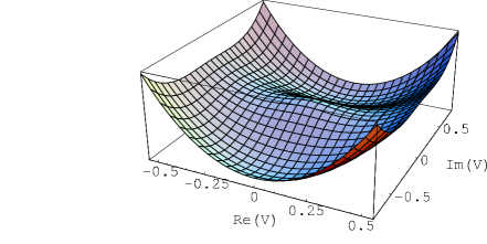
Figure 1: $e^{-G}$ exhibits a local maximum at $V=0$ for negative $\beta$.

Observe that adding a cubic polynomial (and in particular a linear term) in $V$ to (4.2) does not affect the leading behavior of (4.3) near $V=0$.

Next, we compute the metric on the moduli space near $V=0$. Using

$$g_{V\bar{V}}=\partial_{V}\partial_{\bar{V}}G=-e^{G}\,\partial_{V}\partial_{\bar{V}}e^{-G}+G_{V}\,G_{\bar{V}}{\,},$$ (4.4)

and taking $V\rightarrow 0$, we find $G_{V}=-e^{G}\partial_{V}e^{-G}\rightarrow 0$ and

$$g_{V\bar{V}}\approx\frac{\beta}{\pi}\,e^{G_{0}}\,\log\lvert V\rvert^{2}{\,}.$$ (4.5)

Note that the result (4.5) depends crucially on having $\operatorname{Re}a>0$. Furthermore, for the metric to be positive definite as $V\rightarrow 0$, the constant $\beta$ has to be negative.

We also compute the gauge couplings associated with (4.2) near $V\approx 0$. Using [27]

$$g_{IJ}^{-2}=\frac{i}{4}\left(\mathcal{N}_{IJ}-\bar{\mathcal{N}}_{IJ}\right),\qquad\mathcal{N}_{IJ}=\bar{F}_{IJ}+2i\,\frac{\operatorname{Im}F_{IK}\operatorname{Im}F_{JL}Y^{K}Y^{L}}{\operatorname{Im}F_{MN}Y^{M}Y^{N}}{\,},$$ (4.6)

we find, upon diagonalization, that one of the gauge couplings remains approximately constant, while the other coupling exhibits a logarithmic running,

$$g^{-2}\approx\operatorname{Re}a,\;\;{\,},\;\;\;{\tilde{g}}^{-2}\approx\frac{\beta}{4\pi}\log\lvert V\rvert^{2}{\,}.$$ (4.7)

Observe that for negative $\beta$, the coupling ${\tilde{g}}$ becomes small as $V\rightarrow 0$.

The basic example (4.2), with $\beta=-1/2$, describes the conifold singularity of the mirror quintic in type IIB with $V=\psi-1$ (cf. (A.13)) [21, 28]. The metric (4.5) is precisely the metric at the conifold point $\psi=1$ (see table 2 of [21]). Since the conifold singularity is associated with the appearance of one additional massless hypermultiplet [29], we see that we have entropy maximization when a hypermultiplet becomes massless at the singularity. Note that the character of the extremum of the entropy (2.1) at $V=0$ is independent of the value of $Y^{0}_{\mathrm{f}}$.

Next, consider the resolved conifold in type IIA. The associated $\mathcal{F}^{(0)}$ is described by (4.2) with $\beta=-1/2$ and $a=0$ (cf. (A.13)) [13]. We compute the Kähler metric and the gauge coupling in the associated field theory. We decouple gravity by restoring Planck’s mass in (2.3) with $G/M^{2}_{\mathrm{Pl}}$ and $z^{A}/M_{\mathrm{Pl}}$, and by expanding both sides of (2.3) in powers of $M^{-2}_{\mathrm{Pl}}$ [30],

$$G={\hat{K}}(z,{\bar{z}})+f(z)+{\bar{f}}({\bar{z}})+\mathcal{O}(M^{-2}_{\mathrm{Pl}}){\,},$$ (4.8)

where

$${\hat{K}}=-\left({\bar{z}}^{A}\,\mathcal{F}_{A}+z^{A}{\bar{\mathcal{F}}}_{A}\right).$$ (4.9)

Using (4.2), we obtain near $V=-iz^{1}\rightarrow 0$,

$${\hat{K}}\approx\frac{2\beta}{\pi}\lvert V\rvert^{2}\log\lvert V\rvert{\,}.$$ (4.10)

Computing the corresponding Kähler metric near $V\rightarrow 0$ yields

$$g_{V{\bar{V}}}=\partial_{V}\partial_{\bar{V}}{\hat{K}}\approx\frac{2\beta}{\pi}\log\lvert V\rvert{\,},$$ (4.11)

which is positive definite for $\beta<0$. The gauge coupling is computed from (4.6) with $\mathcal{N}_{IJ}={\bar{F}}_{IJ}$ [31]. We obtain

$${\tilde{g}}^{-2}=\frac{i}{4}\left({\bar{F}}_{11}-F_{11}\right)\approx\frac{\beta}{4\pi}\log\lvert V\rvert^{2}{\,},$$ (4.12)

in agreement with (4.7).

More generally, whenever the singularity in moduli space is such that a sufficiently large number of (charged) hypermultiplets becomes massless there, so that the resulting $\beta$ is negative, the function (2.3) exhibits a local maximum. Examples thereof are singularities associated with the appearance of non-abelian gauge symmetries with a non-asymptotically free spectrum [22, 23]. A concrete example is provided by the so-called heterotic $S-T$ model, which is a two-Kähler moduli model with a dual type IIA description in terms of a hypersurface of degree 12 in weighted projective space $P^{4}_{(1,1,2,2,6)}$ with Euler characteristic $\chi=-252$ [32]. The type IIA dual description is based on (A.2) with $V=S-T$ and $n_{0,1}=2$. From (A.7) and (A.9) we infer that $\beta=-1$ and that $a$ is positive. At $V=0$, a gauge symmetry enhancement takes place, whereby a $U(1)$ group is enlarged to an $SU(2)$, with four additional (charged) hypermultiplets becoming massless there [22, 23]. The entropy of axion-free black holes in this model does indeed have a maximum at $S=T$ (cf. eq. (4.34) in [33]).

5 Entropy maximization in the presence of $R^{2}$-interactions

Next, let us discuss entropy maximization in the presence of higher-curvature interactions encoded in $F(Y,\Upsilon)$. Usually, the quantity $F(Y,\Upsilon)$ is assumed to have a perturbative expansion of the form

$$F(Y,\Upsilon)=\sum_{g=0}^{\infty}F^{(g)}(Y)\,\Upsilon^{g}{\,}.$$ (5.1)

Then, expanding the entropy (2.7) in terms of the coupling functions $F^{(g)}(Y)$ yields

$$\begin{split}\mathcal{S}/\pi&=\lvert Y^{0}\rvert^{2}\,e^{-G(z,{\bar{z}})}-2i\Upsilon\left(F^{(1)}-{\bar{F}}^{(1)}\right)-i\Upsilon(z^{A}-{\bar{z}}^{A})\left(\frac{{\bar{Y}}^{0}}{Y^{0}}\,\frac{\partial F^{(1)}}{\partial z^{A}}+\frac{{Y}^{0}}{{\bar{Y}}^{0}}\,\frac{\partial{\bar{F}}^{(1)}}{\partial{\bar{z}}^{A}}\right)\\ &\quad+2i\sum_{g=2}^{\infty}F^{(g)}(Y)\,\Upsilon^{g}\left(-g+(1-g)\,\frac{{\bar{Y}}^{0}}{Y^{0}}\right)-2i\sum_{g=2}^{\infty}{\bar{F}}^{(g)}({\bar{Y}})\,\Upsilon^{g}\left(-g+(1-g)\,\frac{{Y}^{0}}{{\bar{Y}}^{0}}\right)\\ &\quad-i(z^{A}-{\bar{z}}^{A})\sum_{g=2}^{\infty}\Upsilon^{g}\left(\frac{{\bar{Y}}^{0}}{Y^{0}}\,\frac{\partial F^{(g)}}{\partial z^{A}}+\frac{{Y}^{0}}{{\bar{Y}}^{0}}\,\frac{\partial{\bar{F}}^{(g)}}{\partial{\bar{z}}^{A}}\right),\end{split}$$ (5.2)

where $G(z,{\bar{z}})$ is given in (2.3).

Let us first discuss the effect of the gravitational coupling function $F^{(1)}$ on the maximization of the entropy. Let us again consider a singularity of the type (4.2) associated with a vanishing modulus $V=-iz^{1}=-iY^{1}/Y^{0}$, while the other moduli are non-vanishing and kept fixed. From (A.11) it follows that $F^{(1)}$ takes the form

$$F^{(1)}\approx-\frac{i}{64\cdot 12\pi}\beta\,\log V$$ (5.3)

near $V=0$. We compute (using $\Upsilon=-64$)

$$-2i\Upsilon\left(F^{(1)}-{\bar{F}}^{(1)}\right)=4\operatorname{Im}\left(\Upsilon\,F^{(1)}\right)=\frac{\beta}{3\pi}\log\lvert V\rvert{\,},$$ (5.4)

which for negative $\beta$ reaches a maximum as $V\rightarrow 0$, i.e. $\operatorname{Im}\left(\Upsilon\,F^{(1)}\right)\rightarrow+\infty$.

On the other hand, the term proportional to $F^{(1)}_{1}$ in (5.2) only contributes with the phases of $Y^{0}$ and $Y^{1}$,

$$-i\Upsilon(z^{1}-{\bar{z}}^{1})\left(\frac{{\bar{Y}}^{0}}{Y^{0}}\,\frac{\partial F^{(1)}}{\partial z^{1}}+\frac{{Y}^{0}}{{\bar{Y}}^{0}}\,\frac{\partial{\bar{F}}^{(1)}}{\partial{\bar{z}}^{1}}\right)=\frac{\beta}{6\pi}\left(\cos(2\theta_{0})-\cos(2\theta_{1})\right),$$ (5.5)

where $Y^{0}=\lvert Y^{0}\rvert\,\exp(i\theta_{0})$ and $Y^{1}=\lvert Y^{1}\rvert\,\exp(i\theta_{1})$.

We conclude that, for negative $\beta$, not only does $e^{-G}$ have a maximum at $V=0$, but also the $R^{2}$-corrected entropy (5.2) based on $F^{(0)}$ and $F^{(1)}$. Moreover, the contribution of the coupling function $F^{(1)}$ is such that it enhances the maximization of the entropy.

The gravitational coupling function $F^{(1)}$ (as well as the higher $F^{(g)}$) is known to receive non-holomorphic corrections [34, 35]. For instance, for the quintic threefold [34] (and up to an overall constant),

$$\operatorname{Re}F^{(1)}=\log\left(g^{-1}_{\psi{\bar{\psi}}}\,e^{\frac{62}{3}K}\,\lvert\psi^{\frac{62}{3}}\,(1-\psi^{5})^{-\frac{1}{6}}\rvert^{2}\right).$$ (5.6)

Near $V=-iz\equiv\psi-1\approx 0$, $K=\text{constant}$ and $g_{\psi{\bar{\psi}}}\sim-\log\lvert V\rvert$ [21], so that

$$\operatorname{Re}F^{(1)}\sim-\log(-\log\lvert V\rvert)-{\textstyle\frac{1}{6}}\log\lvert V\rvert^{2}{\,}.$$ (5.7)

Therefore, as $V\rightarrow 0$, the behavior of the non-holomorphic term is less singular than the behavior of the holomorphic term, and it can be dropped from the maximization analysis.

Let us express $V=-iY^{1}/Y^{0}$ in terms of the charges $q_{0},q_{1},p^{0}$ and $p^{1}$ by solving the attractor equations (3.1). We take $\mathcal{F}^{(0)}$ to be given by (4.2) and $F^{(1)}$ to be given by (5.3). For simplicity, we take $Y^{1}$ to be imaginary and $Y^{0}$ to be real, so that $V$ is real. Then $Y^{1}=i\,p^{1}/2$, and $Y^{0}$ is determined by

$$4(\operatorname{Re}a)(Y^{0})^{2}+q_{0}Y^{0}+\frac{\beta}{6\pi}-\frac{\beta}{4\pi}(p^{1})^{2}=0{\,}.$$ (5.8)

A large value of $Y^{0}$ can be obtained by choosing $\lvert q_{0}\rvert$ to be large (assuming $\operatorname{Re}a\neq 0$), whereas a small value of $V$ can be achieved by sending $p^{1}\rightarrow 0$. Observe that taking $Y^{0}$ to be fixed at a large value is natural, since (5.1) is based on the perturbative expansion of the topological string free energy, and $Y^{0}$ is related to the inverse topological string coupling constant by $Y^{0}=2\pi\,g_{\mathrm{top}}^{-1}$ (cf. (A.26)).

Next, let us discuss the effect of the higher $F^{(g)}$ (with $g\geq 2$) on the maximization of the entropy. It is known that the higher $F^{(g)}$ also exhibit a singular behavior at $V=0$. For concreteness, we consider the conifold singularity of the mirror quintic [21]. Near the conifold point $z=Y^{1}/Y^{0}\rightarrow 0$ [35, 28],

$$F^{(g)}(Y)=i\frac{A_{g}}{(Y^{0})^{2g-2}\,z^{2g-2}}{\,},\qquad g\geq 2{\,},$$ (5.9)

where $A_{g}$ denote real constants which are expressed [28] in terms of the Bernoulli numbers $B_{2g}$ and are alternating in sign. (cf. (A.28)).

Inserting (5.9) into (5.2) yields

$$\begin{split}\mathcal{S}/\pi&=\lvert Y^{0}\rvert^{2}\,e^{-G(z,{\bar{z}})}-2i\Upsilon\left(F^{(1)}-{\bar{F}}^{(1)}\right)-i\Upsilon(z-{\bar{z}})\left(\frac{{\bar{Y}}^{0}}{Y^{0}}\,\frac{\partial F^{(1)}}{\partial z}+\frac{{Y}^{0}}{{\bar{Y}}^{0}}\,\frac{\partial{\bar{F}}^{(1)}}{\partial{\bar{z}}}\right)\\ &\quad-2\sum_{g=2}^{\infty}A_{g}\,\Upsilon^{g}\,(Y^{1})^{2-2g}\,\left(-g+(1-g)\,\frac{{\bar{Y}}^{1}}{Y^{1}}\right)\\ &\quad-2\sum_{g=2}^{\infty}A_{g}\,\Upsilon^{g}\,({\bar{Y}}^{1})^{2-2g}\left(-g+(1-g)\,\frac{{Y}^{1}}{{\bar{Y}}^{1}}\right).\end{split}$$ (5.10)

We observe that the contribution from the higher $F^{(g)}$ ($g\geq 2$) to (5.10) does not cancel out. This is problematic, since the $F^{(g)}$ become increasingly singular as $z\rightarrow 0$. For instance, when taking $Y^{1}$ to be purely imaginary, the combination $\Upsilon^{g}(Y^{1})^{2-2g}$ is negative for all $g\geq 2$, and the total contribution of the higher $F^{(g)}$ to the entropy does not have a definite sign due to the alternating sign of $B_{2g}$. On the other hand, if we take $Y^{1}$ to be real, then the total contribution of the higher $F^{(g)}$ to the entropy is positive, since the combination $A_{g}\Upsilon^{g}$ is positive for all $g\geq 2$. This contribution becomes infinitely large at $Y^{1}=0$. Thus, to get a better handle on the behavior of the entropy in the presence of higher-curvature corrections near the conifold point $V=0$, it is best to use the non-perturbative expression for $F(Y,\Upsilon)$ for the conifold given in [12, 9], rather than to rely on the perturbative expansion (5.1). This will be done next.

For the resolved conifold in type IIA, $F(Y,\Upsilon)$ is given by (see appendix A) [12, 9],

$$F(Y,\Upsilon)=-C\,\sum_{n=1}^{\infty}n\log\left(1-q^{n}Q\right),$$ (5.11)

where we neglected the $Q$-independent terms, since they do not affect the extremization with respect to $Q$. Here $q=e^{-g_{\mathrm{top}}}$ and $Q=e^{-2\pi V}$. We impose the physical restrictions $\operatorname{Re}g_{\mathrm{top}}>0$ and $\operatorname{Re}V\geq 0$. The topological string coupling constant $g_{\mathrm{top}}$ and the constant $C$ are expressed in terms of $Y^{0}$ and of $\Upsilon$ via (A.26).

Under the assumption of uniform convergence, inserting (5.11) into (2.7) yields the entropy

$$\mathcal{S}=-\sum_{n=1}^{\infty}\operatorname{Re}\left(\frac{nq^{n}Q\log q\bigl{[}n\log q+2\log\lvert Q\rvert\bigr{]}}{\log\bar{q}\,(1-q^{n}Q)}+\frac{n\bigl{[}nq^{n}Q\log q-2(1-q^{n}Q)\log(1-q^{n}Q)\bigr{]}}{1-q^{n}Q}\right).$$ (5.12)

In order to determine the nature of the extrema of (5.12) we numerically approximated this expression by a finite sum of a sufficiently large number of terms. To improve the accuracy of the approximation, the summation was performed in the order of decreasing $n$, so that subsequent summands were of comparable magnitude to the partial sums.

Let us first consider the case when $g_{\mathrm{top}}$ (and hence $q$) is taken to be real. We find that the entropy attains a maximum at $Q=1$, i.e. at the conifold point $V=0$, regardless of the strength of the coupling $g_{\mathrm{top}}$, as displayed in Fig. 2. Observe that the maximum at $Q=1$ occurs at the boundary of the allowed domain, where derivative tests do not directly apply. $\mathcal{S}(q,Q)$ is periodic in $\arg(Q)=-\operatorname{Im}(2\pi V)$.

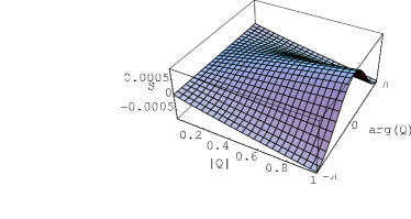
Figure 2: $\mathcal{S}$ as a function of $Q$ for $g_{\mathrm{top}}=0.001$ (left) and $g_{\mathrm{top}}=10$ (right). The conifold point corresponds to $\lvert Q\rvert=e^{-\operatorname{Re}(2\pi V)}=1$ and $\arg(Q)=-\operatorname{Im}(2\pi V)=0$. The number of terms taken into account was 100001 and 1001, respectively.

As the string coupling becomes weaker, the convergence of the series slows down, and the number of terms needed to be taken into account grows roughly proportionally to the inverse coupling, independently of $Q$. This is shown in Fig. 3. We observe that apart from the magnitude, the value of $g_{\mathrm{top}}$ has little influence on the shape of $\mathcal{S}(q,Q)$.

Figure 3: Sums of the first $N$ terms (partial sums) of (5.12) for $g_{\mathrm{top}}=0.001$ (left) and $g_{\mathrm{top}}=10$ (right) at the conifold point $V=0$ ($Q=1$).

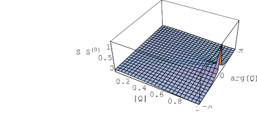
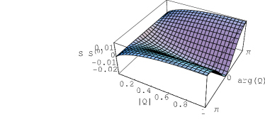
Figure 4: $\mathcal{S}-\mathcal{S}^{(0)}$ as a function of $Q$ for $g_{\mathrm{top}}=0.001$ (left) and $g_{\mathrm{top}}=10$ (right).

Next, let us subtract the tree-level contribution to the entropy, $\mathcal{S}^{(0)}$, computed from

$$F^{(0)}=C\,g_{\mathrm{top}}^{-2}\,\operatorname{Li}_{3}(Q){\,},$$ (5.13)

so as to exhibit the contribution to the entropy from the higher-curvature corrections. The tree-level contribution can be written as

$$\mathcal{S}^{(0)}=\frac{2\operatorname{Re}\bigl{[}\operatorname{Li}_{3}(Q)-\log\lvert Q\rvert\,\operatorname{Li}_{2}(Q)\bigr{]}}{\lvert\log q\rvert^{2}}{\,}.$$ (5.14)

When treated as a function of $Q$ for a fixed $q$ (observe that $\mathcal{S}^{(0)}$ does not depend on $\arg(g_{\mathrm{top}})$), $\mathcal{S}^{(0)}$ has a shape similar to the shape of $\mathcal{S}$.

The difference $\mathcal{S}-\mathcal{S}^{(0)}$ amounts to the contribution to the entropy of the higher-curvature terms. It depends on $Q$ and $g_{\mathrm{top}}$, as can be seen in Fig. 4. At the conifold point $V=0$, the difference $\mathcal{S}-\mathcal{S}^{(0)}$ is positive for small coupling $g_{\mathrm{top}}$, whereas it becomes negative for large values of $g_{\mathrm{top}}$. At weak coupling higher-order corrections become negligible. At strong coupling the corrections, albeit smaller, are comparable to $\mathcal{S}^{(0)}$ and negative, resulting in $\mathcal{S}\ll\mathcal{S}^{(0)}$ ($\mathcal{S}^{(0)}$ decreases as $g_{\mathrm{top}}^{-2}$, while $\mathcal{S}$ decreases as $g_{\mathrm{top}}e^{-g_{\mathrm{top}}}$ for large $g_{\mathrm{top}}$). This is displayed in Fig. 5, where we plotted $(\mathcal{S}-\mathcal{S}^{(0)})/\mathcal{S}$.

Figure 5: The ratio $(\mathcal{S}-\mathcal{S}^{(0)})/\mathcal{S}$ as a function of $g_{\mathrm{top}}$ or $q$ at $Q=1$.

Finally, if we allow $g_{\mathrm{top}}$ to be complex the behavior of $\mathcal{S}$ changes markedly. As $\operatorname{Re}(V)$ tends to zero, we notice increasingly pronounced oscillations, whose amplitude and period sensitively depend on $g_{\mathrm{top}}$ (see Fig. 6). In effect, the maximum formerly at $V=0$ is displaced and new local extrema appear.

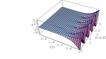
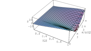
Figure 6: $\mathcal{S}$ as a function of $Q$ for complex $g_{\mathrm{top}}$. Left: $g_{\mathrm{top}}=0.01-0.7i$, right: $g_{\mathrm{top}}=0.01+3i$. Note that the range of $\arg(Q)$ in the 3-dimensional graphs has been cut by half to exhibit the point $Q=1$ more clearly (but the periodicity remains $2\pi$). The 2-dimensional graphs show in greater detail the edges of the surfaces closest to the viewer (cross-sections through the surfaces along $\arg(Q)=0$ and $\lvert Q\rvert=1$).

Note that the entropy (5.12) is not necessarily positive, because we have not included the contribution stemming from the Euler characteristic of the Calabi–Yau threefold (see (A.9)) and of other moduli (which, if present, we have taken to be constant).

6 Relation to OSV free energy

According to [14], the entropy (2.7) can be rewritten as

$$\mathcal{S}=E-L{\,},$$ (6.1)

where $E$ denotes the OSV free energy which, in the conventions of [36], reads

$$E=4\pi\operatorname{Im}{F}{\,},$$ (6.2)

and where $L$ is given by

$$L=\pi\,q_{I}\,\phi^{I}=4\pi\operatorname{Im}F_{I}\operatorname{Re}Y^{I}$$ (6.3)

by virtue of the attractor equations

$$q_{I}=4\,\frac{\partial\operatorname{Im}F}{\partial\phi^{I}}$$ (6.4)

with $\phi^{I}=2\operatorname{Re}Y^{I}$.

The function $F(Y,\Upsilon)$ is related to the topological partition function $F_{\mathrm{top}}$ by $F(Y,\Upsilon)=-iF_{\mathrm{top}}/(2\pi)$ (see (A.25) and (A.26) with $\Upsilon=-64$). Using $E=-(F_{\mathrm{top}}+\bar{F}_{\mathrm{top}})$ and

$$Z_{\mathrm{top}}=e^{-F_{\mathrm{top}}}{\,},$$ (6.5)

we obtain

$$e^{\mathcal{S}}=\lvert Z_{\mathrm{top}}\rvert^{2}\,e^{-L}{\,}.$$ (6.6)

For the resolved conifold in type IIA, the free energy $E$ and $L$, computed from (5.11), are given by

$$\begin{split}E&=2\sum_{n=1}^{\infty}n\operatorname{Re}\left(\log(1-q^{n}Q)\right){\,},\\ L&=2\sum_{n=1}^{\infty}n\left[\operatorname{Im}\left(\frac{q^{n}Q\log q}{1-q^{n}Q}\right)\operatorname{Im}\left(\frac{\log Q}{\log q}\right)\right.\\ &\qquad\qquad\;+\left.\operatorname{Re}\left(\frac{1}{\log q}\right)\operatorname{Re}\left(\frac{q^{n}Q\log q(n\log q+\log Q)}{1-q^{n}Q}\right)\right].\end{split}$$ (6.7)

By numerically approximating these expressions as before, we find that for real coupling $g_{\mathrm{top}}$, the OSV free energy $E$ is minimized at the conifold point $Q=1$, see Fig. 7. The entropy $\mathcal{S}$ is maximized at the conifold, as discussed before.

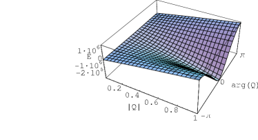
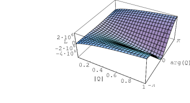
Figure 7: $E$ and $L$ as functions of $Q$ for $g_{\mathrm{top}}=0.001$ (compare with the left graph in Fig. 2).

At the conifold point, $E$ and $L$ as functions of real $q$ have the behaviour displayed in Fig. 8. In the limit $g_{\mathrm{top}}\rightarrow 0$, we thus find that at the conifold point,

$$E=\frac{1}{2}L=-\mathcal{S}{\,}$$ (6.8)

(which holds for the sums, but not term by term). Hence, at the conifold point,

$$e^{\mathcal{S}}=\lvert Z_{\mathrm{top}}\rvert^{-2}{\,}.$$ (6.9)

Observe that (6.9) is in agreement with (6.6) at the conifold point.

Figure 8: Ratios $E/L$ and $E/\mathcal{S}$ at the conifold point, plotted as functions of real $q$.

The relation (6.9) can also be derived from the prepotential $\mathcal{F}^{(0)}$ given in (4.2), as follows. At $V=0$, by (2.1) and (4.3),

$$\mathcal{S}=2\pi\,\lvert Y^{0}\rvert^{2}\,\left(\mathcal{F}^{(0)}+{\bar{\mathcal{F}}}^{(0)}\right).$$ (6.10)

Taking $Y^{0}$ to be real (which corresponds to real $g_{\mathrm{top}}$), and using $F=-i(Y^{0})^{2}\,\mathcal{F}^{(0)}$, we compute the OSV free energy (6.2) and find precisely

$$E=-\mathcal{S}{\,}.$$ (6.11)

7 Conclusions

We have discussed entropy maximization with respect to one complex modulus at points in moduli space at which an excess of hypermultiplets becomes massless. We found that the function $e^{-G(z,{\bar{z}})}$ exhibits a local maximum at such points. When taking into account the gravitational coupling $F^{(1)}$, the maximization is further enhanced due to the additional term $\operatorname{Im}(\Upsilon F_{\Upsilon})$ in the entropy (2.7) representing the departure from the area law. The inclusion of the higher $F^{(g)}$-couplings into the maximization analysis is, however, problematic due to their singular nature at these points in moduli space. This problem can be circumvented by resorting to the non-perturbative expression for the topological free energy, rather than relying on its genus expansion. We did so in the case of the resolved conifold, where we found that the conifold point is a maximum of the entropy for real topological string coupling, but ceases to be a maximum once the topological string coupling is taken to be complex. Note that when performing the maximization analysis we kept $Y^{0}$ fixed throughout moduli space as in [9]. Other choices are, in principle, possible and could modify the results concerning the maximization of the entropy.

Appendix A Normalization of $F(Y,\Upsilon)$

In type IIA, $F^{(0)}(Y)$ has the following expansion [21, 37, 38, 39]

$$F^{(0)}(Y)=(Y^{0})^{2}\left(-\frac{C_{ABC}z^{A}z^{B}z^{C}}{6}+h(z)-\frac{1}{(2\pi i)^{3}}\sum_{d_{A}}n_{d}\,\operatorname{Li}_{3}(e^{2\pi id_{A}z^{A}})\right),$$ (A.1)

where $C_{ABC}$ are the intersection numbers and $n_{d}$ denote rational instanton numbers. The quadratic polynomial $h(z)$ contains a constant term given by $i\,\chi\,\zeta(3)/(2(2\pi)^{3})$, where $\chi$ denotes the Euler characteristic. Using (2.2) yields

$$\mathcal{F}^{(0)}(z)=-\frac{i}{6}C_{ABC}z^{A}z^{B}z^{C}+ih(z)+\frac{1}{(2\pi)^{3}}\sum_{d_{A}}n_{d}\,\operatorname{Li}_{3}(e^{2\pi i\,d_{A}z^{A}}){\,}.$$ (A.2)

Observe that in the limit of large positive $\operatorname{Im}z^{A}$, $e^{-G(z,{\bar{z}})}$ (computed from (2.3)) is positive, as it should.

The coupling function $F^{(1)}(Y)$ is given by [34, 37, 39]

$${F}^{(1)}(Y)=-\frac{i}{256\pi}\left[-\frac{2\pi i}{12}c_{2A}\,z^{A}-\sum_{d_{A}}\left(2n^{(1)}_{d}\log(\eta(e^{2\pi id_{A}z^{A}}))+\frac{n_{d}}{6}\log(1-e^{2\pi id_{A}z^{A}})\right)\right].$$ (A.3)

Consider a singularity associated with the vanishing of one of the moduli $T^{A}=-iz^{A}$. We denote this modulus by $V$. The other moduli are taken to be large, so that we may approximate

$$\sum_{d_{A}}n_{d}\,\operatorname{Li}_{3}(e^{-2\pi d_{A}T^{A}})\approx\sum_{d_{V}}n_{0,0,\dotsc,d_{V}}\,\operatorname{Li}_{3}(e^{-2\pi d_{V}V}){\,}.$$ (A.4)

Let us assume that that the only non-vanishing instanton number $n_{0,0,\dotsc,d_{V}}$ is the one with $d_{V}=1$. Using

$$\operatorname{Li}_{3}(e^{-x})=\zeta(3)-\frac{\pi^{2}}{6}x+\left(\frac{3}{4}-\frac{1}{2}\log x\right)x^{2}+\mathcal{O}(x^{3}){\,},$$ (A.5)

we find that for $V\approx 0$, the function $\mathcal{F}^{(0)}$ can be approximated by

$$\mathcal{F}^{(0)}=-\frac{C_{ABC}T^{A}T^{B}T^{C}}{6}+i{\tilde{h}}(iT)+\frac{\beta}{2\pi}V^{2}\log V{\,},$$ (A.6)

where

$$\beta=-\frac{n_{0,0,\dotsc,1}}{2}{\,}.$$ (A.7)

The instanton number $n_{0,0,\dotsc,1}$ counts the difference of charged hyper- and vector multiplets becoming massless at $V=0$, i.e.

$$n_{0,0,\dotsc,1}=n_{\mathrm{h}}-n_{\mathrm{v}}{\,}.$$ (A.8)

Note that the quadratic polynomial $i\tilde{h}$ contains a constant term $a$ given by

$$a=(2-\chi)\,\frac{\zeta(3)}{2(2\pi)^{3}}{\,}.$$ (A.9)

Similarly, we find that near $V=0$,

$${F}^{(1)}(Y)=-\frac{i}{256\pi}\left[\frac{2\pi}{12}c_{2A}\,T^{A}-2\sum_{d_{A}}n^{(1)}_{d}\log(\eta(e^{-2\pi d_{A}T^{A}}))+\frac{\beta}{3}\log V\right].$$ (A.10)

Therefore, near $V=0$ we obtain

$$\begin{split}F(Y,\Upsilon)&=\sum_{g=0}^{\infty}F^{(g)}(Y)\Upsilon^{g}=F^{(0)}(Y)+F^{(1)}(Y)\Upsilon+\dotsb\\ &=-\frac{i(Y^{0})^{2}}{2\pi}\beta\,V^{2}\log V-\frac{i\Upsilon}{64\cdot 12\pi}\beta\,\log V+\dotsb{\,},\end{split}$$ (A.11)

where we displayed only the terms proportional to $\log V$.

The function $F(Y,\Upsilon)$ is proportional to the topological free energy $F_{\mathrm{top}}(g_{\mathrm{top}},z)$. In order to determine the precise relation between supergravity and topological string quantities, we consider the case of the resolved conifold in type IIA. First, observe that for this case the functions $\mathcal{F}^{(0)}$ and $F^{(1)}$ are given by [13]

$$\begin{split}\mathcal{F}^{(0)}&=-\frac{V^{3}}{12}+ih(iV)+\frac{1}{(2\pi)^{3}}\sum_{n}\frac{e^{-2\pi nV}}{n^{3}}{\,},\\ {F}^{(1)}&=-\frac{i}{256\pi}\left[\frac{2\pi}{12}\,c_{2}\,V-\frac{1}{6}\log(1-e^{-2\pi V})\right],\end{split}$$ (A.12)

where $h(iV)$ denotes a quadratic polynomial in $V$, and where $c_{2}=-1$. Observe that $\chi=2$, so that $a=0$. Using (A.5) and (A.9), it follows that near $V=0$,

$$\begin{split}\mathcal{F}^{(0)}&\approx-\frac{1}{4\pi}V^{2}\log V{\,},\\ {F}^{(1)}&\approx\frac{i}{128\cdot 12\pi}\log V{\,}.\end{split}$$ (A.13)

Then, comparison with (A.6) and (A.10) yields $\beta=-1/2$.

The topological free energy for the resolved conifold reads [12, 9]

$$F_{\mathrm{top}}=-\sum_{n=1}^{\infty}n\log(1-q^{n}Q){\,},$$ (A.14)

where $q=e^{-g_{\mathrm{top}}}$ and $Q=e^{-t}$, and where we neglected the $Q$-independent terms. We now review the standard argument leading to the expansion of $F_{\mathrm{top}}$ in powers of $g_{\mathrm{top}}$. Using the Laurent expansions

$$\log(1-z)=-\sum_{k=1}^{\infty}\frac{z^{k}}{k}{\,},\qquad\lvert z\rvert<1{\,},$$ (A.15)

and

$$\sum_{n=1}^{\infty}nz^{n}=\frac{z}{(1-z)^{2}}{\,},\qquad\lvert z\rvert<1{\,},$$ (A.16)

we obtain for $\lvert q^{k}Q\rvert<1$ and $\lvert q^{k}\rvert<1$,

$$F_{\mathrm{top}}=\sum_{n=1}^{\infty}\sum_{k=1}^{\infty}\frac{nq^{kn}Q^{k}}{k}=\sum_{k=1}^{\infty}\frac{q^{k}Q^{k}}{k(1-q^{k})^{2}}=\sum_{k=1}^{\infty}\frac{Q^{k}}{4k\sinh^{2}(kg_{\mathrm{top}}/2)}{\,}.$$ (A.17)

The conditions $\lvert q^{k}\rvert<1$ and $\lvert q^{k}Q\rvert<1$ imply that $\operatorname{Re}g_{\mathrm{top}}>0$ and $\operatorname{Re}t>-\operatorname{Re}g_{\mathrm{top}}$, the former condition being automatically satisfied for physical coupling and the latter being fulfilled when $\operatorname{Re}t$ is interpreted as the volume of the two-cycle.

The expression (A.17) can be further rewritten with the help of Bernoulli numbers $B_{n}$, defined by

$$\frac{z}{e^{z}-1}=\sum_{n=0}^{\infty}B_{n}\frac{z^{n}}{n!}{\,},\qquad\lvert z\rvert<2\pi{\,},$$ (A.18)

and satisfying

$$B_{2n+1}=0\quad(n>0),\qquad B_{2n}=(-1)^{n-1}\lvert B_{2n}\rvert{\,}.$$ (A.19)

The first few values are $B_{0}=1$, $B_{1}=-1/2$, $B_{2}=1/6$ and $B_{4}=-1/30$. Subtracting from (A.18) its derivative multiplied by $z$ we obtain

$$\frac{(z/2)^{2}}{\sinh^{2}(z/2)}=B_{0}+\sum_{n=1}^{\infty}B_{n}\frac{(1-n)z^{n}}{n!}{\,},$$ (A.20)

and so, by virtue of the properties of $B_{n}$,

$$F_{\mathrm{top}}=\sum_{k=1}^{\infty}\frac{Q^{k}}{k^{3}}\left(g_{\mathrm{top}}^{-2}+\sum_{g=1}^{\infty}(-1)^{g}\,\frac{(2g-1)}{(2g)!}\lvert B_{2g}\rvert k^{2g}g_{\mathrm{top}}^{2g-2}\right).$$ (A.21)

This can be written in terms of the polylogarithms

$$\operatorname{Li}_{s}(z)=\sum_{k=1}^{\infty}\frac{z^{k}}{k^{s}}{\,},\qquad\lvert z\rvert<1{\,},$$ (A.22)

as

$$F_{\mathrm{top}}=g_{\mathrm{top}}^{-2}\,\operatorname{Li}_{3}(e^{-t})+\sum_{g=1}^{\infty}(-1)^{g}\,\frac{(2g-1)}{(2g)!}\,\lvert B_{2g}\rvert\,g_{\mathrm{top}}^{2g-2}\,\operatorname{Li}_{3-2g}(e^{-t}){\,}.$$ (A.23)

In the limit $t\rightarrow 0$, we obtain [28]

$$\begin{split}F_{\mathrm{top}}&=-\frac{1}{2}\left(\frac{t}{g_{\mathrm{top}}}\right)^{2}\log t+\frac{1}{12}\log t-\sum_{g\geq 2}^{\infty}\frac{B_{2g}}{2g(2g-2)}\left(\frac{g_{\mathrm{top}}}{t}\right)^{2g-2}\\ &\quad+g_{\mathrm{top}}^{-2}\,\zeta(3)+\sum_{g\geq 2}^{\infty}(-1)^{g}\,\frac{(2g-1)}{(2g)!}\,\lvert B_{2g}\rvert\,g_{\mathrm{top}}^{2g-2}\,\zeta(3-2g){\,},\end{split}$$ (A.24)

where we made use of the identity $\operatorname{Li}_{s}(1)=\zeta(s)$.

Observe that when deriving (A.23) the expansion (A.18) was used, which is valid under the condition $\lvert z\rvert<2\pi$, or $\lvert kg_{\mathrm{top}}\rvert<2\pi$. In (A.17), however, this condition is satisfied only up to a certain integer $k$. The result (A.24) is therefore not rigorous. A careful analysis of the asymptotic expansion at weak topological coupling $g_{\mathrm{top}}$ has been given in [40, 41].

Finally, substituting $t=2\pi V$ and comparing (A.24) with (A.11) yields

$$F(Y,\Upsilon)=CF_{\mathrm{top}}(g_{\mathrm{top}},z)$$ (A.25)

with

$$\begin{split}C&=\frac{i\,\Upsilon}{128\pi}{\,},\\ g_{\mathrm{top}}^{2}&=-\frac{\pi^{2}\Upsilon}{16(Y^{0})^{2}}{\,},\end{split}$$ (A.26)

where we used $\beta=-1/2$.

For the conifold, it follows from (A.24) and (A.26) that in the limit $V=-iY^{1}/Y^{0}\rightarrow 0$, the higher coupling functions $F^{(g)}(Y)$ are given by

$$F^{(g)}(Y)=i\frac{A_{g}}{(Y^{1})^{2g-2}}{\,},\qquad g\geq 2{\,},$$ (A.27)

where

$$A_{g}=-\frac{4^{2-2g}}{256\pi}\,\frac{B_{2g}}{g(2g-2)}{\,}.$$ (A.28)

Observe that the coefficients $A_{g}$ are alternating in sign.

References

- [1] S. Ferrara, R. Kallosh and A. Strominger, extremal black holes, Phys. Rev. D52 (1995) 5412–5416 [hep-th/9508072].
- [2] A. Strominger, Macroscopic entropy of extremal black holes, Phys. Lett. B383 (1996) 39–43 [hep-th/9602111].
- [3] S. Ferrara and R. Kallosh, Supersymmetry and attractors, Phys. Rev. D54 (1996) 1514–1524 [hep-th/9602136].
- [4] H. Ooguri, C. Vafa and E. P. Verlinde, Hartle–Hawking wave-function for flux compactifications, Lett. Math. Phys. 74 (2005) 311–342 [hep-th/0502211].
- [5] G. Curio, A. Klemm, D. Lüst and S. Theisen, On the vacuum structure of type II string compactifications on Calabi–Yau spaces with -fluxes, Nucl. Phys. B609 (2001) 3–45 [hep-th/0012213].
- [6] K. Behrndt, G. L. Cardoso and D. Lüst, Curved BPS domain wall solutions in four-dimensional supergravity, Nucl. Phys. B607 (2001) 391–405 [hep-th/0102128].
- [7] F. Denef and M. R. Douglas, Distributions of flux vacua, JHEP 05 (2004) 072 [hep-th/0404116].
- [8] R. Kallosh, Flux vacua as supersymmetric attractors, hep-th/0509112.
- [9] S. Gukov, K. Saraikin and C. Vafa, The entropic principle and asymptotic freedom, hep-th/0509109.
- [10] K. Behrndt et al., Classical and quantum supersymmetric black holes, Nucl. Phys. B488 (1997) 236–260 [hep-th/9610105].
- [11] G. L. Cardoso, B. de Wit and T. Mohaupt, Corrections to macroscopic supersymmetric black-hole entropy, Phys. Lett. B451 (1999) 309–316 [hep-th/9812082].
- [12] R. Gopakumar and C. Vafa, M-theory and topological strings. I, hep-th/9809187.
- [13] R. Gopakumar and C. Vafa, On the gauge theory/geometry correspondence, Adv. Theor. Math. Phys. 3 (1999) 1415–1443 [hep-th/9811131].
- [14] H. Ooguri, A. Strominger and C. Vafa, Black hole attractors and the topological string, Phys. Rev. D70 (2004) 106007 [hep-th/0405146].
- [15] B. de Wit, P. G. Lauwers, R. Philippe, S. Q. Su and A. Van Proeyen, Gauge and matter fields coupled to N=2 supergravity, Phys. Lett. B134 (1984) 37.
- [16] B. de Wit and A. Van Proeyen, Potentials and symmetries of general gauged N=2 supergravity-Yang–Mills models, Nucl. Phys. B245 (1984) 89.
- [17] A. Strominger, Special geometry, Commun. Math. Phys. 133 (1990) 163–180.
- [18] S. Bellucci, S. Ferrara and A. Marrani, On some properties of the attractor equations, hep-th/0602161.
- [19] S. Ferrara, G. W. Gibbons and R. Kallosh, Black holes and critical points in moduli space, Nucl. Phys. B500 (1997) 75–93 [hep-th/9702103].
- [20] B. Fiol, On the critical points of the entropic principle, hep-th/0602103.
- [21] P. Candelas, X. C. De La Ossa, P. S. Green and L. Parkes, A pair of Calabi–Yau manifolds as an exactly soluble superconformal theory, Nucl. Phys. B359 (1991) 21–74.
- [22] A. Klemm and P. Mayr, Strong coupling singularities and non-abelian gauge symmetries in string theory, Nucl. Phys. B469 (1996) 37–50 [hep-th/9601014].
- [23] S. Katz, D. R. Morrison and M. R. Plesser, Enhanced gauge symmetry in type II string theory, Nucl. Phys. B477 (1996) 105–140 [hep-th/9601108].
- [24] R. M. Wald, Black hole entropy is the Noether charge, Phys. Rev. D48 (1993) 3427–3431 [gr-qc/9307038].
- [25] D. Gaiotto, A. Strominger and X. Yin, New connections between 4D and 5D black holes, JHEP 02 (2006) 024 [hep-th/0503217].
- [26] K. Behrndt, G. L. Cardoso and S. Mahapatra, Exploring the relation between 4D and 5D BPS solutions, Nucl. Phys. B732 (2006) 200–223 [hep-th/0506251].
- [27] B. de Wit, V. Kaplunovsky, J. Louis and D. Lüst, Perturbative couplings of vector multiplets in heterotic string vacua, Nucl. Phys. B451 (1995) 53–95 [hep-th/9504006].
- [28] D. Ghoshal and C. Vafa, string as the topological theory of the conifold, Nucl. Phys. B453 (1995) 121–128 [hep-th/9506122].
- [29] A. Strominger, Massless black holes and conifolds in string theory, Nucl. Phys. B451 (1995) 96–108 [hep-th/9504090].
- [30] N. Seiberg and E. Witten, Electric-magnetic duality, monopole condensation, and confinement in supersymmetric Yang–Mills theory, Nucl. Phys. B426 (1994) 19–52 [hep-th/9407087].
- [31] B. de Wit, Special geometry and perturbative analysis of heterotic vacua, hep-th/9511019.
- [32] S. Kachru and C. Vafa, Exact results for compactifications of heterotic strings, Nucl. Phys. B450 (1995) 69–89 [hep-th/9505105].
- [33] K. Behrndt, G. L. Cardoso and I. Gaida, Quantum supersymmetric black holes in the model, Nucl. Phys. B506 (1997) 267–292 [hep-th/9704095].
- [34] M. Bershadsky, S. Cecotti, H. Ooguri and C. Vafa, Holomorphic anomalies in topological field theories, Nucl. Phys. B405 (1993) 279–304 [hep-th/9302103].
- [35] M. Bershadsky, S. Cecotti, H. Ooguri and C. Vafa, Kodaira–Spencer theory of gravity and exact results for quantum string amplitudes, Commun. Math. Phys. 165 (1994) 311–428 [hep-th/9309140].
- [36] G. L. Cardoso, B. de Wit, J. Käppeli and T. Mohaupt, Black hole partition functions and duality, hep-th/0601108.
- [37] P. Candelas, X. De La Ossa, A. Font, S. Katz and D. R. Morrison, Mirror symmetry for two parameter models. I, Nucl. Phys. B416 (1994) 481–538 [hep-th/9308083].
- [38] S. Hosono, A. Klemm, S. Theisen and S. T. Yau, Mirror symmetry, mirror map and applications to Calabi–Yau hypersurfaces, Commun. Math. Phys. 167 (1995) 301–350 [hep-th/9308122].
- [39] S. Hosono, A. Klemm, S. Theisen and S. T. Yau, Mirror symmetry, mirror map and applications to complete intersection Calabi–Yau spaces, Nucl. Phys. B433 (1995) 501–554 [hep-th/9406055].
- [40] A. Dabholkar, F. Denef, G. W. Moore and B. Pioline, Exact and asymptotic degeneracies of small black holes, JHEP 08 (2005) 021 [hep-th/0502157].
- [41] A. Dabholkar, F. Denef, G. W. Moore and B. Pioline, Precision counting of small black holes, JHEP 10 (2005) 096 [hep-th/0507014].