A solution to the 4-tachyon off-shell amplitude in cubic string field theory

Abstract:

We derive an analytic series solution of the elliptic equations providing the 4-tachyon off-shell amplitude in cubic string field theory (CSFT). From such a solution we compute the exact coefficient of the quartic effective action relevant for time dependent solutions and we derive the exact coefficient of the quartic tachyon coupling. The rolling tachyon solution expressed as a series of exponentials $e^{t}$ is studied both using level-truncation computations and the exact 4-tachyon amplitude. The results for the level truncated coefficients are shown to converge to those derived using the exact string amplitude. The agreement with previous work on the subject, both on the quartic tachyon coupling and on the CSFT rolling tachyon, is an excellent test for the accuracy of our off-shell solution.

1 Introduction and Conclusions

Cubic string field theory (CSFT) [1] has played an important role in recent years in describing the dynamics of the open bosonic string tachyon. Both the unstable vacuum and the true vacuum where the tachyon has condensed have been shown to be well-defined states in CSFT [2]. Tachyon condensation is an off-shell process and string field theory is the natural setting for its analysis. The condensation process should be described by the solutions of the equation of motion of the tachyon effective action which can be constructed perturbatively in string field theory. The tachyon effective action in fact can be derived from the off-shell tachyon amplitudes, which can be computed in various ways in string field theory. Following the classification of ref.[3], there are four possible approaches for computing off-shell amplitudes that we briefly describe here since three of them have been used in this paper.

a)

Field theory approach

The string field contains an infinite number of component fields, whose number grows exponentially with the mass level $L$. In this approach one can approximate the calculations by truncating the string field up to some fixed level $L$ [4], for this reason it is called “level truncation on fields”. For example one can construct the CSFT lagrangian by means of a truncated string field up to some level $L$ and then compute the cubic terms for each of the field components at the desired level. From this classical action one can then derive the tree level effective action for some field component ($e.g.$ the tachyon) by integrating out all the other ones through the solution of their equations of motion. We shall use this procedure in Sections 4-5 to derive the perturbative tachyon effective action.

b)

Conformal mapping

With this method Giddings [5] reproduced the on-shell Veneziano amplitude directly from Witten’s CSFT. He gave an explicit conformal map that takes the Riemann surfaces defined by the Witten diagrams to the standard disc with four tachyon vertex operators on the boundary. Following Giddings’ procedure and with some additional analysis -related to the oscillator method in c)- Samuel [6] and Sloan [7] computed the off-shell Veneziano amplitude. This procedure allows in principle the calculation of any amplitude [8]. Amplitudes computed using this method are exact, although numerical approximations are necessary to get concrete numbers for them. We shall solve Samuel’s equations to derive, from the 4-tachyon off shell amplitude, some very accurate numerical approximations of the quartic coupling of the tachyon potential and of a time dependent solution of CSFT.

c)

Oscillator method

Perturbative amplitudes can be directly evaluated using the oscillator representation of the vertices and propagators in CSFT. The vertex and the propagator can be written completely in terms of squeezed states [9], i.e. in terms of exponentials of quadratic forms in the oscillators creating and annihilating operators. In this way the complete set of amplitudes associated with a Feynmann diagram results in an integral over the internal momenta that can be evaluated using standard squeezed techniques (see Section 2). Any perturbative amplitude is then given in a closed-form expression containing infinite-dimensional Neumann matrices. While no analytical way is known at present to exactly calculate such expressions, one can evaluate the amplitudes to a high degree of precision truncating the Neumann matrices to finite size [10]. This means truncate the levels of oscillators in the string states which are considered, this is the reason for which this method is known as “level truncation on oscillators”. Rather then having to include a number of fields which grows exponentially in the level, with this procedure one simply needs to evaluate quantities, as the determinant of the Neumann matrices, whose size grows linearly in the truncation level. A specific example of this method is given in Appendix B.

d)

Moyal string field theory

In this alternative formulation of SFT the string joining star product is identified with the Moyal product. Calculations performed using this method reproduce directly the expressions for the off-shell amplitudes as for example the $3$-point and $4$-point tachyon amplitudes [11]. Some numerical results [12] achieved with this procedure are comparable to those obtained using the methods (a)-(c).

In this paper we mainly focus on the four tachyon amplitude which we evaluate both by solving explicitly Samuel’s elliptic equations for the off-shell factor (method (b)) and by level truncation (methods (a) and (c)). In particular we have obtained a new series solution for the off-shell factor introduced by Samuel [6], which, at variance with the one found in [11], provides the off-shell factor in terms of the original coordinates used in [6]. From this solution we shall then extract off-shell information both on the non-perturbative stable vacuum and on the tachyon dynamics.

As a test for the solution we shall first improve the numerical approximation for the evaluation of the exact quartic self-coupling $c_{4}$ in the tachyon potential. This was computed for the first time in [4] and repeated to a higher degree of precision in [10]. Our results provides $c_{4}$ with a precision that goes up to the ninth significative digit and is in complete agreement with the extrapolations of ref. [13].

As a second application we shall improve the CSFT time-dependent solution given in [14] as a sum in powers of $e^{t}$.

Since Sen’s seminal paper on the rolling tachyon [15], much work has been devoted to the study of time dependent solutions in string theory [16, 17, 18, 19, 20, 14]. The setting is realized by considering a system of unstable $D$-branes which decays in time as the tachyon field rolls down from the maximum of the potential towards the stable minimum. A review on previous work on this problem is given in [2].

The dynamics of a rolling tachyon has been studied in various frameworks. The physical picture emerging from the boundary states, RG flow and boundary string field theory (BSFT) approaches [21, 17, 22] is quite clear. The tachyon rolls from the perturbative to the true vacuum, which is reached in an infinite time. The same physical picture can also be obtained following other approaches, among them the analysis involving DBI-type actions [23, 24, 25, 26], S-branes and time-like Liouville theory [27, 28, 29, 30, 31], matrix models [32, 33, 34, 35, 36, 37], cubic superstring field theory [38], vacuum SFT [39, 40, 41] and fermionic boundary CFT [42].

CSFT instead fails to provide a meaningful description of the rolling tachyon dynamics. At the lowest order, the $(0,0)$, in the level truncation scheme one considers only the tachyon field and the cubic string field theory action becomes

$$S={1\over g_{\rm o}^{2}}\int d^{26}x\left({1\over 2}\,\phi(x)\,(\Box+1)\,\phi(x)-{1\over 3}\lambda\left(\lambda^{(1/3)\Box}\phi(x)\right)^{3}\right),$$ (1)

where the coupling $\lambda$ has the value $\lambda=3^{9/2}/2^{6}=2.19213$. Considering spatially homogeneous profiles of the form $\phi(t)$, where $t$ is time, the equation of motion derived from (1) is

$$(\partial_{t}^{2}-1)\phi(t)+\lambda^{1-\partial_{t}^{2}/3}\left(\lambda^{-\partial_{t}^{2}/3}\phi(t)\right)^{2}=0.$$ (2)

This equation was studied in [18, 19, 20, 14]. In [20] it was found an almost exact well behaved solution of this equation for $\lambda<1$. The solution has interesting analytical properties and is remarkably simple. The “evolution” of the solution to different values of $\lambda$ is driven by a diffusion equation which makes Eq.(2) local with respect to the time variable $t$. The analytic continuation of this solution to the physical value $\lambda=3^{9/2}/2^{6}$ can be performed for any time $t$ with the exception of a single point, $t=0$, where the solution is not analytic. The profile can be expressed in terms of a series in powers of $e^{t}$ for $t<0$ and in powers of $e^{-t}$ for $t>0$ and in this way it is well-behaved except at the origin where it has a cusp. Alternatively, one can extend to positive $t$ the solution in powers of $e^{t}$ and the solution presents ever-growing oscillations. In any case the tachyon always rolls well past the minimum of the potential then turns around. Solutions with ever-growing oscillations have been found also in refs. [18, 19, 14]. In [14], in particular, a systematic level-truncation analysis was carried out for a trajectory $\phi(t)$ expressed as a power series in $e^{t}$. It was also shown that the non-local field redefinition, which takes the CSFT action to the BSFT action [43], also maps the wildly oscillating CSFT solution to the well-behaved BSFT exponential solution. Increasing the level of truncation in CSFT or the number of terms retained in the tachyon effective action leads to a well defined trajectory at least up to some upper bound in $t$, $t=t_{b}$. In fact, if the position of the first turnaround points, that the solution exhibits for $t>0$, tends to stabilize as the truncation level $L$ of the effective action increases, the expansion in powers of $e^{t}$ for $t>0$ would be justified at least up to those points [14]. For the first turnaround points, the leading terms in the CSFT solution are those with small powers of $e^{t}$. Consequently, the very accurate value of the 4-tachyon amplitude that we have found in this paper improves the solution of ref. [14], at least up to the first extrema of the trajectory.

The trajectories $\phi(t)$, obtained by computing the $\phi^{4}$ term in the effective action exactly and the terms up to $\phi^{7}$ in an $L=2$ approximation, show that indeed the position of the first turnaround point does not change significantly with the improvement in the $\phi^{4}$ term. This suggests the possibility that this value actually has the physical meaning of inversion point. The second turnaround point instead changes position and amplitude compared to the one found in [14]. The inclusion of higher order terms in the lagrangian however does not produce significative changes, so that the trajectory seems again to stabilize. Thus we confirm that for $t>0$, the tachyon does not roll towards the stable non-perturbative minimum of the potential and that the qualitative behavior of wild oscillations is reproduced even if the amplitudes at the turnaround points beyond the first are sensibly diminished.

The solutions of the 4-tachyon off-shell amplitude that we have found therefore is a very useful tool for providing precise tests of CSFT. The agreement with previous work on the subject, both on the quartic tachyon coupling and on the CSFT rolling tachyon, is an excellent test for the accuracy of our off-shell solution.

As for the DBI tachyon action, it would be instructive to study the cubic tachyonic action on a curved background and, in particular, in a Friedmann Robertson Walker (FRW) spacetime. It would be interesting to see if the coupling of the free theory to a Friedman-Robertson-Walker metric [44], and the consequent inclusion of a Hubble friction term, might lead from the classical solution with ever-growing oscillations to damped oscillations around the stable minimum of the potential well. Cubic string field theory might then open interesting perspectives in tachyon cosmology [45].

The paper is organized as follows. In Section 2 we review the derivation of the off-shell four tachyon amplitude following ref. [6]. Explicit formulas for the Neumann coefficients involved in the oscillator formalism are reported in Appendix A. A brief review of the level truncation method is also given and a specific example is provided in Appendix B. In Section 3 we develop the tools needed to perform the computations of Sections 4-5. A solution to the elliptic equations defining the off-shell amplitude is derived, obtaining a useful expansion of $\kappa(x)$ in powers of the Koba-Nielsen variable $x$. This analysis improves the accuracy in the evaluation of the quartic coupling of the tachyon potential, which is performed in Section 4. Finally, in Section 5 we use the exact four-point amplitude to study the first few coefficients of the rolling tachyon solution expressed as a sum of exponentials $e^{nt}$, and we compare the corresponding solution with the ones obtained in the level truncation scheme.

Our calculations were performed using the symbolic manipulation program Mathematica.

2 Off-shell 4-tachyon amplitude

The first step in computing the off-shell four tachyon amplitude in CSFT is to construct the Feynman diagrams directly from the cubic interaction vertex. Four-point amplitudes involve one propagator and two vertices. After gauge fixing, we use the Feynman-Siegel gauge, the propagator becomes $b_{0}/L_{0}$ where $L_{0}$ is the Virasoro generator for the intermediate state including ghosts

$$L_{0}=p\cdot p-1+\sum_{n=1}^{\infty}\left(\alpha_{-n}\cdot\alpha_{n}+nb_{-n}c_{n}+nc_{-n}b_{n}\right)\,\,.$$ (3)

Writing the propagator

$${b_{0}\over L_{0}}=b_{0}\int_{0}^{\infty}dTe^{-TL_{0}}\;,$$

$e^{-TL_{0}}$ inserts a world-sheet strip of length $T$ into the amplitude.

2.1 Conformal mapping: on-shell amplitude

A closed analytical expression for the off-shell four tachyon amplitude in CSFT [1] was derived in [6] by following Gidding’s analysis of the on-shell Veneziano amplitude [5]. Giddings gave an explicit conformal map that takes the Riemann surfaces defined by the Witten diagrams to the standard disc with four tachyon vertex operators on the boundary. This conformal map is defined in terms of four parameters $\alpha,~{}\beta,~{}\gamma,~{}\delta$. The four parameters are not independent variables. They satisfy the relations

$$\alpha\beta=1\quad\quad\gamma\delta=1$$ (4)

and

$${1\over 2}=\Lambda_{0}(\theta_{1},k)-\Lambda_{0}(\theta_{2},k)\;,$$ (5)

where $\Lambda_{0}(\theta,k)$ is defined by

$$\Lambda_{0}(\theta,k)={2\over\pi}\left(E(k)F(\theta,k^{\prime})+K(k)E(\theta,k^{\prime})-K(k)F(\theta,k^{\prime})\right)\;\;.$$ (6)

In (6) $K(k)$ and $E(k)$ are complete elliptic functions of the first and second kinds, $F(\theta,k)$ is the incomplete elliptic integral of the first kind (we follow the notation of ref.[46]). The parameters $\theta_{1}$, $\theta_{2}$, $k$ and $k^{\prime}$ satisfy

$$k^{2}={\gamma^{2}\over\delta^{2}} k^{\prime 2}=1-k^{2}$$ (7)

$$\sin^{2}\theta_{1}={\beta^{2}\over\beta^{2}+\gamma^{2}} \sin^{2}\theta_{2}={\alpha^{2}\over\alpha^{2}+\gamma^{2}}\,.$$ (8)

By convention $\beta>\alpha$ and $\delta>\gamma$. Because of (4) and (5) only one variable is independent. By convention this is taken to be $\alpha$, that is related to $T$, the lenght of the intermediate strip, by

$${T\over 2}=K(k^{\prime})\left[Z(\theta_{2},k^{\prime})-Z(\theta_{1},k^{\prime})\right]$$ (9)

where $Z(\theta,k)$ is defined through the ordinary elliptic functions

$$Z(\theta,k)=K(k)E(\theta,k)-E(k)F(\theta,k)\;.$$ (10)

The parameter $\alpha$ is finally related to the Koba-Nielsen variable $x$ through

$$x=\left({(1-\alpha^{2})\over(1+\alpha^{2})}\right)^{2}\ ,~{}~{}~{}~{}~{}~{}~{}~{}~{}~{}~{}~{}~{}~{}\alpha=\sqrt{{1-\sqrt{x}\over 1+\sqrt{x}}}\ .$$ (11)

Using this conformal map Giddings managed to derive the Veneziano amplitude from CSFT. Because of the cubic vertex, in CSFT there are six relevant Feynman diagrams for four particles processes (fig.1). The contribution from the graph (a) in fig.1 was computed in [5] to be

$$A_{s}(p_{1},p_{2},p_{3},p_{4})=\int_{\alpha_{0}}^{0}d\alpha\,2A_{G}~{}{dT\over d\alpha}~{}(\beta-\alpha)^{2(p_{1}\cdot p_{2}+p_{3}\cdot p_{4})}(\beta+\alpha)^{2(p_{1}\cdot p_{3}+p_{2}\cdot p_{4})}(2\alpha)^{2(p_{2}\cdot p_{3})}(2\beta)^{2(p_{1}\cdot p_{4})}$$ (12)

where the integration limits $\alpha_{0}=\sqrt{2}-1$ and $\alpha=0$ correspond to $T=0$ and $T=\infty$ respectively , $2A_{G}$ is the ghost contribution and is given by

$$2A_{G}=8{1\over 2\pi}\sqrt{\alpha^{2}+\gamma^{2}}\sqrt{\beta^{2}+\gamma^{2}}(\beta^{2}-\alpha^{2})K(\gamma^{2})$$ (13)

and the Jacobian factor almost cancels the ghost factor

$${dT\over d\alpha}=-{4(\beta^{2}-\alpha^{2})\over\alpha A_{G}}~{}~{}~{}~{}~{}.$$ (14)

Figure 1: The relevant Feynman diagrams for the four particles scattering.

2.2 Oscillator method: off-shell amplitude

Samuel derived a perturbative off-shell string amplitude [6] directly from string field theory by requiring that it reproduces Gidding’s result (12) when the momenta are set on-shell. We now briefly review Samuel results.

Let

$${g\over 2}\langle{V^{(3)}_{41I}}|\langle{V^{(3)}_{23J}}|b_{0}e^{-TL_{0}}|V^{(2)}_{IJ}\rangle=\,\langle{V^{(4)}_{1234}}|$$ (15)

denote the vertex function associated with the graph (a) in fig.1, where the subscripts $1,2,3,4,I$ and $J$ indicate Fock-space labels. The full contribution to the diagram is

$$\int_{0}^{\infty}dT\langle{V^{(4)}_{1234}}||\Psi^{(4)}_{4}\,\rangle|\Psi^{(3)}_{3}\rangle|\Psi^{(2)}_{2}\rangle|\Psi^{(1)}_{1}\rangle$$ (16)

where $|\Psi^{(r)}_{r}\rangle$ is the Fock-space representation of the external states. The explicit oscillator representations of $\langle{V^{(2)}}|$ and $\langle{V^{(3)}}|$

$$\langle{V^{(2)}_{12}}|=\int d^{26}p\;\langle{p}|^{(1)}\otimes\langle{p}|^{(2)}\left(c_{0}^{(1)}+c_{0}^{(2)}\right)e^{-\sum_{n=1}^{\infty}(-1)^{n}\left[a_{n}^{(1)}\cdot a_{n}^{(2)}+c_{n}^{(1)}b_{n}^{(2)}+c_{n}^{(2)}b_{n}^{(1)}\right]}$$ (17)

$$\langle{V^{(3)}_{123}}|= \int d^{26}p_{1}d^{26}p_{2}d^{26}p_{3}\;\delta(p_{1}+p_{2}+p_{3})\langle{p_{1}}|^{(1)}c_{0}^{(1)}\otimes\langle{p_{2}}|^{(2)}c_{0}^{(2)}\otimes\langle{p_{3}}|^{(3)}c_{0}^{(3)}\cdot$$ (19)

$$\cdot e^{-{1\over 2}\sum_{r,s=1}^{3}\left[a_{m}^{(r)}V_{mn}^{rs}a_{n}^{(s)}+2a_{m}^{(r)}V^{rs}_{m0}p^{(s)}+p^{(r)}V^{rs}_{00}p^{(s)}-2c_{m}^{(r)}X_{mn}^{rs}b_{n}^{(s)}\right]}$$

show that all the terms in (16) are given in terms of exponentials of quadratic expressions in the oscillators. Using standard squeezed state techniques [9], closed-form expressions can be given for any perturbative amplitude. In the case of the four tachyon amplitude corresponding to the first diagram of fig.1, this procedure gives

$$A_{4}(p_{1},p_{2},p_{3},p_{4})\!=\!{\lambda_{c}^{2}g^{2}\over 2}\,\delta(\textstyle{\sum_{i}}p_{i})\!\int_{0}^{\infty}dT\,e^{T}\,{\rm det}\left(\textstyle{{1-(\tilde{X}^{11})^{2}\over 1-(\tilde{V}^{11})^{2}}}\right)e^{-{1\over 2}p_{i}Q^{ij}p_{j}}$$ (20)

where $\lambda_{c}$ is a constant related to the Neumann coefficient for the three tachyon vertex, $\lambda_{c}=e^{3V_{00}^{11}}={3^{9/2}\over 2^{6}}$ . In this formula $\tilde{V}^{11}$ and $\tilde{X}^{11}$ are defined by

$$\tilde{V}^{11}_{mn}=e^{-{(m+n)\over 2}T}V^{11}_{mn}\;\;\;\;\;\;\;\;\;\tilde{X}^{11}_{mn}=e^{-{(m+n)\over 2}T}X^{11}_{mn}$$ (21)

where $V^{rs}$ and $X^{rs}$ are infinite-dimensional matrices

$$V^{rs} =\left(\begin{array}[]{ccccc}V^{rs}_{11}&V^{rs}_{12}&\dots&V^{rs}_{mn}&\dots\\ V^{rs}_{21}&V^{rs}_{22}&\dots&V^{rs}_{m+1,n}&\dots\\ \dots&\dots&\dots&\dots&\dots\end{array}\right), X^{rs} =\left(\begin{array}[]{ccccc}X^{rs}_{11}&X^{rs}_{12}&\dots&X^{rs}_{mn}&\dots\\ X^{rs}_{21}&X^{rs}_{22}&\dots&X^{rs}_{m+1,n}&\dots\\ \dots&\dots&\dots&\dots&\dots\end{array}\right)$$ (28)

whose elements are matter and ghost Neumann coefficients of the cubic string field theory vertex, for which exact expressions are given in the Appendix A. $Q^{ij}$ are defined as

$$Q^{ij}= V^{iI}_{0m}\left(\textstyle{{1\over 1-(\tilde{V}^{11})^{2}}}\right)_{mn}\tilde{V}^{11}_{np}V^{Ij}_{p0}+V_{00}^{11}-T(2-\delta_{ij})\;\;\;\;\;\;i,j=1,2\;\hbox{or}\;i,j=3,4$$ (29)

$$Q^{ij}= -V^{iI}_{0m}\left(\textstyle{{1\over 1-(\tilde{V}^{11})^{2}}}\right)_{mn}\,C\,\tilde{V}^{11}_{np}V^{Ij}_{p0}\quad\;\;\;\;\;\;i=1,2\;\hbox{and}\;j=3,4\;\hbox{or}\;i=3,4\;\hbox{and}\;j=1,2$$ (30)

where $m,n,p\geq 1$, $C=\delta_{mn}(-1)^{n}$ and the sum over $I$ denotes a sum over the intermediate states.

The two expressions (12) and (20) should both represent the contribution to the four tachyon amplitude coming from the diagram (a) in fig.1 when the momenta are on-shell. To relate them in the proper way, a general procedure was developed in [6] for computing the functions $Q^{ij}$ appearing in (20) from the Giddings map, giving

$$Q^{11} =Q^{44}=\ln\alpha-\ln\kappa, Q^{22}=Q^{33} =-\ln\alpha-\ln\kappa$$

$$Q^{12} =Q^{21}=-\ln|\alpha-\beta|, Q^{13}=Q^{31} =-\ln(\alpha+\beta)$$

$$Q^{14} =Q^{41}=-\ln(2\beta), Q^{23}=Q^{32} =-\ln(2\alpha)$$

$$Q^{24} =Q^{42}=-\ln(\alpha+\beta), Q^{34}=Q^{43} =-\ln|\alpha-\beta|$$ (32)

where $\kappa$ is given as an integral

$$\ln(\kappa)=-2\alpha\textstyle{{(\beta^{2}-\alpha^{2})\over\sqrt{(\alpha^{2}+\gamma^{2})(\alpha^{2}+\delta^{2})}}}\int_{1}^{\infty}\!\!dw\ln(w-1){d\over dw}\left(\textstyle{{\sqrt{(w^{2}+\alpha^{2}\gamma^{2})(w^{2}+\alpha^{2}\delta^{2})}\over(w+1)(\beta^{2}w^{2}-\alpha^{2})}}\right)\;\;.$$ (33)

As already noticed, although $\alpha,\beta,\gamma,\delta$ all appear in the above equation, there is only one independent variable, so that the function $\kappa$ in (35) is actually a function of $\alpha$. The substitution of (32) in (20) leads to the following formula

$$A_{4}(p_{1},p_{2},p_{3},p_{4}) = \lambda_{c}^{2}{g^{2}\over 2}\int_{\alpha_{0}}^{0}d\alpha{dT\over d\alpha}e^{T}{\rm det}\left(\textstyle{{1-(\tilde{X}^{11})^{2}\over 1-(\tilde{V}^{11})^{2}}}\right)\left[\kappa(\alpha)\right]^{\sum_{i=1}^{4}p^{2}_{i}}\left(\alpha\right)^{-(p_{1}^{2}+p_{4}^{2})+p_{2}^{2}+p_{3}^{2}}$$ (35)

$$|\alpha-\beta|^{2(p_{1}\cdot p_{2}+p_{3}\cdotp_{4})}(\beta+\alpha)^{2(p_{1}\cdot p_{3}+p_{2}\cdotp_{4})}(2\alpha)^{2(p_{2}\cdot p_{3})}(2\beta)^{2(p_{1}\cdot p_{4})}$$

Comparing the two expressions (12) and (35) on shell ($p^{2}_{i}=1$), one can see that the momentum dependence matches and for the momentum independent part the following identity holds

$$\lambda_{c}^{2}\left({dT\over d\alpha}\right)e^{T}{\rm det}\left(\textstyle{{1-(\tilde{X}^{11})^{2}\over 1-(\tilde{V}^{11})^{2}}}\right)=2A_{g}{dT\over d\alpha}{1\over\left[\kappa(\alpha)\right]^{4}}\;\;.$$ (36)

By trading the variable $\alpha$ for the Koba-Nielsen variable $x$ through (11) in (35), the contribution from the first graph in fig.1 becomes

$$A_{4}(p_{1},p_{2},p_{3},p_{4})={g^{2}\over 2}\int_{{1\over 2}}^{1}dx\;x^{p_{1}\cdot p_{2}+p_{3}\cdot p_{4}}(1-x)^{(p_{1}+p_{4})^{2}-2}\left({\kappa(x)\over 2}\right)^{\sum_{i=1}^{4}p^{2}_{i}-4}$$ (37)

The remaining diagrams (b),(c),(d),(e),(f) of fig.1 can be obtained from the first one by a suitable permutation of the string labels, i.e. by permuting the momenta in (37), and the total four-point tachyon amplitude is the sum of these six contributions. Notice that the Veneziano amplitude is exactly reproduced when $p^{2}_{i}=1$ in (37) and the additional factor containing $\kappa(x)$ goes to $1$.

2.3 Level truncation

The infinite-dimensional matrices (28) appearing in the final expression for a given diagram are expressed in terms of the Neumann coefficients of Witten’s vertex. The level truncation method we use in this paper consists in the truncation on the level of oscillators associated with the Neumann coefficients. This procedure is somewhat different from the original method of level truncation [4] (method a) section 1), in which one calculates the SFT action by only including in the string field expansion contributions up to a fixed total oscillator level. While the latter approach involves computations with a number of fields that grows exponentially in the level, in the former one has to calculate the determinant of some matrices whose size grows linearly in the truncation level.

Let us explicitly remind the procedure [47] in the case of a tree diagram with four external fields as (20), in which there is a single internal propagator with Schwinger parameter $T$. One starts with a suitable change of coordinates in (20)

$$\sigma=e^{-T}$$ (38)

then expands in powers of $\sigma$, so getting an expression of the form

$$\int_{0}^{1}{d\sigma\over\sigma^{2}}\sigma^{p^{2}}\sum_{n=0}^{\infty}c_{n}(p_{i})\sigma^{n}=\sum_{n=0}^{\infty}{c_{n}(p^{i})\over p^{2}+n-1}\;\;,$$ (39)

where $p=p_{1}+p_{2}=p_{3}+p_{4}$ represents the momentum of the intermediate state. The poles $p^{2}=1-n$ in (39) clearly correspond to the contributions of intermediate particles as the tachyon ($n=0$), the gauge field ($n=1$) and all the other open string massive fields. Truncate all the matrices to size $L\times L$ means to truncate the sum in (39) to $n=L$, thus imposing a limit on the mass of the intermediate states.

The analysis can be simplified by noting that in the four point amplitude the contributions of odd level fields cancel between $s$ and $t$ channels so that only even levels in the truncation, i.e. only even powers of $\sigma$ in the expansion (39), need to be considered. An explicit example of the procedure above explained is given in Appendix B, where the four tachyon amplitude at level $L=2$ is derived in the time-dependent case.

3 Solution for the function $\kappa(x)$

As shown in the previous section the off-shell 4-point string amplitudes are completely determined once the function $\kappa(x)$ defined by (33) is known. To determine the function $\kappa(\alpha,\gamma)$ we have first to solve eq.(5) for one of the two variables in terms of the other, so that the function $\kappa$ will be a function of only one of the two $\alpha$ or $\gamma$. Since the four point amplitude is written in terms of an integral over $x$, which is easily related to $\alpha$ through (11), it would be more natural to solve for $\gamma$ as a function of $\alpha$ then the opposite. The solution can be found numerically and for $\gamma$ as a function of $x$ is given by the solid line in fig.2. $\gamma$ goes from 0 to 1 while $x$ goes from 1 to 1/2 and $\alpha$ goes from 0 to $\sqrt{2}-1$. To check for the accuracy of the solution, we have found two different expansions: 1) A power series in $\alpha$ which gives $\gamma$ in a neighbor of $0$ and can be inverted so as to give $\alpha$ as a function of $\gamma$ around 0. 2) An expansion of $\alpha$ around $\sqrt{2}-1$ as an expansion in $1-\gamma$, this series cannot be inverted due to the presence of terms of the type $(1-\gamma)^{m}\log(1-\gamma)^{n}$. We have found a general procedure to obtain as many terms as necessary in both expansions and the function $\alpha(\gamma)$ can be determined in the whole range $0\leq\gamma\leq 1$. As we shall show in fact the two series for $\alpha(\gamma)$ overlap in an extended interval that goes from $\gamma\sim 0.6$ to $\gamma\sim 0.7$.

3.1 $\gamma$ and $\alpha$ around $0$

By using the integral representations of the elliptic functions [46] it is possible to write the equation (5) in a useful form

$$E(\gamma^{2})\int_{\alpha\gamma}^{\gamma/\alpha}dt{1\over\sqrt{t^{2}+\gamma^{4}}\sqrt{1+t^{2}}}-(1-\gamma^{4})K(\gamma^{2})\int_{\alpha\gamma}^{\gamma/\alpha}dt{1\over\sqrt{t^{2}+\gamma^{4}}(\sqrt{1+t^{2}})^{3}}={\pi\over 4}\;$$ (40)

To expand (40) for small $\gamma$ and $\alpha$ we have to divide the integration region into three intervals in such a way that the square roots in the denominators of (40) can be consistently expanded and the integrals in $t$ performed. For example consider the integral in the first term of (40), it can be rewritten as

$$\int_{\alpha\gamma}^{\gamma/\alpha}dt{1\over\sqrt{t^{2}+\gamma^{4}}\sqrt{1+t^{2}}}=$$ (41)

$$\int_{\alpha\gamma}^{\gamma^{2}}dt{1\over\gamma^{2}\sqrt{1+{t^{2}\over\gamma^{4}}}\sqrt{1+t^{2}}}+\int^{1}_{\gamma^{2}}dt{1\over t\sqrt{1+{\gamma^{4}\over t^{2}}}\sqrt{1+t^{2}}}+\int_{1}^{{\gamma\over\alpha}}dt{1\over t^{2}\sqrt{1+{\gamma^{4}\over t^{2}}}\sqrt{1+{1\over t^{2}}}}$$ (42)

In each integral of the rhs the integration domain is contained in the convergence radius of the Taylor expansions of the square roots containing $\gamma$, so that they can be safely expanded and the integrals in $t$ performed.

With this procedure one gets the following equation equivalent to (40)

$$E(\gamma^{2})\sum_{n,k=0}^{\infty}{{\Gamma({1\over 2})^{2}\over\Gamma({1\over 2}-n)\Gamma({1\over 2}-k)n!k!}}$$ (44)

$$\left\{{2\over 2n+2k+1}\left[\gamma^{4k}-\left({\alpha\over\gamma}\right)^{2n+1}\left(\alpha\gamma\right)^{2k}\right]+\left(1-\delta_{kn}\right){\gamma^{4n}-\gamma^{4k}\over 2k-2n}-\delta_{kn}\gamma^{4n}\ln{\gamma^{2}}\right\}$$ (45)

$$-(1-\gamma^{4})K(\gamma^{2})\sum_{n,k=0}^{\infty}{{\Gamma({1\over 2})\Gamma(-{1\over 2})\over\Gamma({1\over 2}-n)\Gamma(-{1\over 2}-k)n!k!}}$$ (46)

$$\left\{{1\over 2n+2k+1}\left[\gamma^{4k}-\left({\alpha\over\gamma}\right)^{2n+1}\left(\alpha\gamma\right)^{2k}\right]+\left(1-\delta_{kn}\right){\gamma^{4n}-\gamma^{4k}\over 2k-2n}-\delta_{kn}\gamma^{4n}\ln{\gamma^{2}}\right.$$ (47)

$$\left.+{1\over 2n+2k+3}\left[\gamma^{4n}-\left({\alpha\over\gamma}\right)^{2k+3}\left(\alpha\gamma\right)^{2n}\right]\right\}={\pi\over 4}$$ (48)

The series containing $\ln\gamma^{2}$ can be resummed, the first gives ${2\over\pi}K(\gamma^{2})$ the second ${2\over\pi(1-\gamma^{4})}E(\gamma^{2})$. Hence these terms cancel and $\ln\gamma^{2}$ actually disappears from the equation. As a consequence one can write $\gamma$ as a power series in $\alpha$ whose coefficients are determined requiring that eq.(48) is satisfied. $\gamma$ turns out to contain only the powers $\alpha^{4n+1}$, $n\in\mathbb{N}$. We have determined the first 12 terms of this series to get a very good approximation for $\gamma$ in an extended neighbor of zero (in which sense it is an extended neighbor will be clarified later)

$$\gamma=\sqrt{3}\alpha\left(1+5\alpha^{4}+{1041\over 16}\alpha^{8}+{38719\over 32}\alpha^{12}+{109062913\over 4096}\alpha^{16}+{5278728465\over 8192}\alpha^{20}+\right.$$ (49)

$$\left.{2172202186251\over 131072}\alpha^{24}+{116561474500179\over 262144}\alpha^{28}+{3303689940814193505\over 268435456}\alpha^{32}+\right.$$ (50)

$$\left.{187301165958864015157\over 536870912}\alpha^{36}+{86571446884950765378149\over 8589934592}\alpha^{40}+\right.$$ (51)

$$\left.{5078927050639748451791733\over 17179869184}\alpha^{44}+\,O(\alpha^{48})\right)$$ (52)

Any higher order in (52) can be in principle computed from (48). Using (11) we can plot $\gamma$ as a function of $x$ and compare it to the graph obtained from the numerical solution of eq.(40). As it is clear from fig.2 $\gamma(x)$ has in $x=1/2$ a vertical tangent, thus showing the presence of a branch point which cannot be gotten from a power series of the form (52). Nevertheless (52) gives a very good approximation for $\gamma(x)$ except in a small neighbor of $x=1/2$. In particular the agreement between the values of $\gamma$ obtained from the series (52) and the numerical values is on the 15-th significative digit for $0.8\leq x\leq 1$, where the series (52) is expected to give exact results, thus providing a precision test for the accuracy of the numerical solution.

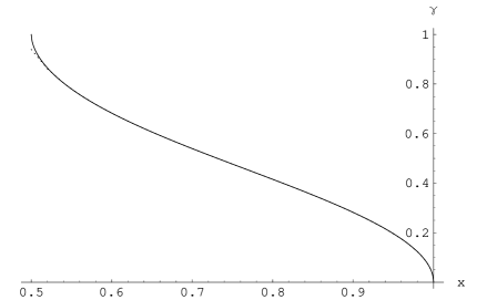
Figure 2: Plots of $\gamma(x)$: the solid line is the numerical solution of the elliptic equation, the dashed line is the power series.

Moreover, the expansion (52) can be iteratively inverted to give a series for $\alpha$ as a function of $\gamma$

$$\alpha={\gamma\over\sqrt{3}}\left(1-{5\over 9}\gamma^{4}+{959\over 1296}\gamma^{8}-{10993\over 7776}\gamma^{12}+{83359631\over 26873856}\gamma^{16}-{3579242677\over 483729408}\gamma^{20}+\right.$$ (53)

$$\left.{1297273056905\over 69657034752}\gamma^{24}-{6783253984031\over 139314069504}\gamma^{28}+{168109910408625655\over 1283918464548864}\gamma^{32}-\right.$$ (54)

$$\left.{24949101849547687507\over 69331597085638656}\gamma^{36}+{10046339553062261150885\over 9983749980331966464}\gamma^{40}-\right.$$ (55)

$$\left.{512861712698825472832315\over 179707499645975396352}\gamma^{44}+O(\gamma^{48})\right)$$ (56)

By plugging the expansion (52) in (33) and using (11), the corresponding expansion for $\kappa(\alpha)$ can be found by means of numerical integration

$$\kappa(\alpha)={8\over 3\sqrt{3}}\;{\rm exp} \!\!\!\!\left[-2.5\,\alpha^{4}-7.1562\,\alpha^{8}-75.927\,\alpha^{12}-1238.7\,\alpha^{16}-24301\,\alpha^{20}\right.$$ (59)

$$\left.-531290\,\alpha^{24}-1.2489\cdot 10^{7}\,\alpha^{28}-3.0923\cdot 10^{8}\,\alpha^{32}\right.$$

$$\left.-7.9627\cdot 10^{9}\,\alpha^{36}-2.1140\cdot 10^{11}\,\alpha^{40}-5.7517\cdot 10^{12}\,\alpha^{44}\right]+O(\alpha^{48})\ .$$

3.2 $\gamma$ around 1 and $\alpha$ around $\sqrt{2}-1$

Around $x=1/2$, i.e $\alpha=\sqrt{2}-1$ and $\gamma=1$, it is possible to obtain only $x$ (or $\alpha$) as a function of $\gamma$ and not the opposite. Such an expansion can be obtained by first expanding eq.(40) around $\gamma=1$ and then looking for an expansion of $\alpha$ in terms of powers of $1-\gamma$ and $\ln(1-\gamma)$

$$\alpha=\sqrt{2}-1+a_{1}(1-\gamma)+a_{2}(1-\gamma)^{2}+\dots+b_{1}(1-\gamma)\ln(1-\gamma)+$$ (61)

$$b_{2}(1-\gamma)^{2}\ln(1-\gamma)+\dots+c_{1}(1-\gamma)(\ln(1-\gamma))^{2}+c_{2}(1-\gamma)^{2}(\ln(1-\gamma))^{2}+\dots$$ (62)

(63)

The coefficients in (63) are determined by requiring that (40) is satisfied. We provide here directly the expansion of $x$ as a function of $1-\gamma$ up to the ninth order

$$x={1\over 2}+{1\over 8}(1-\gamma)^{2}\left[1-2\log\left(\textstyle{{1-\gamma\over 4}}\right)\right]-{1\over 4}(1-\gamma)^{3}\log\left(\textstyle{{1-\gamma\over 4}}\right)-$$ (64)

$${1\over 16}(1-\gamma)^{4}\left[1+3\log\left(\textstyle{{1-\gamma\over 4}}\right)\right]-{1\over 96}(1-\gamma)^{5}\left[7+12\log\left(\textstyle{{1-\gamma\over 4}}\right)\right]+$$ (65)

$${1\over 1536}(1-\gamma)^{6}\left[-97-108\log\left(\textstyle{{1-\gamma\over 4}}\right)-24\log^{2}\left(\textstyle{{1-\gamma\over 4}}\right)+64\log^{3}\left(\textstyle{{1-\gamma\over 4}}\right)\right]-$$ (66)

$${1\over 2560}(1-\gamma)^{7}\left[119+100\log\left(\textstyle{{1-\gamma\over 4}}\right)-40\log^{2}\left(\textstyle{{1-\gamma\over 4}}\right)-320\log^{3}\left(\textstyle{{1-\gamma\over 4}}\right)\right]+$$ (67)

$${1\over 10240}(1-\gamma)^{8}\left[-321-60\log\left(\textstyle{{1-\gamma\over 4}}\right)+1240\log^{2}\left(\textstyle{{1-\gamma\over 4}}\right)+2240\log^{3}\left(\textstyle{{1-\gamma\over 4}}\right)\right]+$$ (68)

$${1\over 107520}(1-\gamma)^{9}\left[-1871+5740\log\left(\textstyle{{1-\gamma\over 4}}\right)+29120\log^{2}\left(\textstyle{{1-\gamma\over 4}}\right)+31360\log^{3}\left(\textstyle{{1-\gamma\over 4}}\right)\right]+\dots$$ (69)

From (56) one can easily get $x$ as a function of $\gamma$ in the region $x\sim 1$ ($\gamma\sim 0$) so that $x(\gamma)$ can be obtained for the whole range $1/2\leq x\leq 1$. The two expansions in fact overlap in a long range for $0.3\leq\gamma\leq 0.7$ as it is shown in fig.3. They have an excellent agreement up to the 13-th significative digit for $0.6\leq\gamma\leq 0.7$.

Figure 3: Plots of $x(\gamma)$: the dashed line gives the expansion of $x(\gamma)$ which holds in a neighbor of $\gamma=1$, the solid line gives the expansion of $x(\gamma)$ around $\gamma=0$.

4 Coefficient of the Quartic Tachyon Potential

The static tachyon potential has the form

$$V_{T}={1\over 2}\phi^{2}-g\,k\,\,\phi^{3}+g^{2}k^{2}\,c_{4}\phi^{4}+\dots$$ (71)

where $g$ is the string coupling constant and $k={3^{7/2}\over 2^{7}}$.

The four point tachyon potential is obtained from the off-shell four tachyon amplitude by setting to zero the external momenta and by explicitly subtracting out the term with the tachyon on the internal line. The amplitude is the sum of the six Feynman diagrams shown in fig.1, the first of which gives the contribution (37) that can be usefully rewritten in terms of the Mandelstam variables

$$A4(s,t,u)={g^{2}\lambda_{c}^{2}\over 2}\int_{{1\over 2}}^{1}\;dx\;x^{{t-s-u\over 2}}(1-x)^{s-2}\left({\kappa(x)\over 2}\right)^{t+s+u-4}\;\;.$$ (72)

To get explicitly the first diagram contribution to the amplitude one can set $t=u=0$ in (72), $A_{4}$ can then be defined through an analitical continuation of (72) to the region $s\leq 1$. This can be achieved by adding and subtracting the pole in $x=1$ in the integrand of (72)

$$\int_{{1\over 2}}^{1}dx\;x^{-{s\over 2}}(1-x)^{s-2}\left({\kappa(x)\over 2}\right)^{s-4}=\int_{{1\over 2}}^{1}dx\;x^{-{s\over 2}}(1-x)^{s-2}\left[\left({\kappa(x)\over 2}\right)^{s-4}-\left({\kappa(1)\over 2}\right)^{s-4}\right]$$ (73)

$$+\left({\kappa(1)\over 2}\right)^{s-4}\int_{{1\over 2}}^{1}\;dx\;x^{-{s\over 2}}(1-x)^{s-2}\;\;.$$ (74)

where the first integral is now well defined in $s=0$. When $\textit{Re}[s]>1$ the last integral in (74) gives

$${2^{s-2}\over\sqrt{\pi}}\Gamma(1-{s\over 2})\Gamma({s\over 2}-{1\over 2})+{2^{2-{s\over 2}}\over s-2}~{}_{2}F_{1}\left(1,2-s;2-{s\over 2};-1\right)$$

that has a well defined limit for $s\to 0$, so that the four point tachyon potential can be written

$$A4(0,0,0)={g^{2}\lambda_{c}^{2}\over 2}\left[\int_{{1\over 2}}^{1}dx\left(\left({2\over\kappa(x)}\right)^{4}-\left({2\over\kappa(1)}\right)^{4}\right)(1-x)^{-2}-{3\over 2}\left({2\over\kappa(1)}\right)^{4}\right]$$ (75)

As already pointed out, the function $\kappa(x)$ in (75) can be evaluated numerically in the whole interval ${1\over 2}<x<1$, by using the numerical solution of eq.(40) graphed in fig.LABEL:gammax. The integrand in (75) is regular at $x=1$, as can be easily checked by studying the behavior of (LABEL:kappasint) in a neighbor of $\alpha=0$. However, problems are expected in the numerical evaluation of the integral in a neighbor of $x=1$ due to the product of a pole times a zero. To circumvent possible computational problems we divided the interval ${1\over 2}<x<1$ into two parts . For $x\in[{1\over 2},0.95]$ we used numerical evaluation of $\kappa(x)$, by plugging the numerical solutions of (40) in (33). For $x\in[0.95,1]$ we used the analitical expression obtained substituting (11) in (LABEL:kappasint). By summing the two contributions we have found the value $A4(0,0,0)=-{g^{2}\over 2}2.94497480(2)$. To get the the quartic term of the tachyon effective potential we have to subtract [4] from (75) the contribution from the internal tachyon line

$$A4_{t}(s,t,u)={g^{2}\over 2}\lambda_{c}^{2-s-{t+u\over 3}}{1\over s-1}$$ (76)

evaluated at $s=t=u=0$. Each graph in fig.1 contributes equally, so that for the quartic tachyon coupling one eventually gets

$$g^{2}k^{2}c_{4}={6\over 4!}\left[A4(0,0,0)-A4_{t}(0,0,0)\right]={6\over 4!}{g^{2}\over 2}(-2.94497480(2)+{3^{9}\over 2^{12}})={g^{2}\over 4!}\;5.5813353(1)$$ (77)

where the factor $1/4!$ is required to recover the units of [48, 10]. The numerical evaluation of the coefficient $c_{4}$ from the exact four tachyon amplitude was given in [6] to an accuracy of $1\%$, $c_{4}\approx 1.75(2)$, and in [10] to an accuracy of $0.1\%$, $c_{4}\approx 1.742(1)$. We have repeated this calculation to an higher degree of precision, and the result (77) gives

$$c_{4}\approx 1.74220008(3)\;.$$ (78)

This coefficient was calculated using the level truncation scheme up to level $L=20$ in [48], and improved up to level $L=28$ in [13], thus obtaining $c_{4,L=28}\simeq-1.70028$, with a discrepancy of $2.4\%$ with respect to (78). In the same paper, a procedure to extrapolate the known level truncated results and predict the asymptotic $L\to\infty$ value for $c_{4}$ was described, giving an extimated value $c_{4,L\to\infty}=1.7422006(9)$ that agrees within the $10^{-7}$ of accuracy with our exact result (78).

5 The rolling tachyon in cubic string field theory

As a second application of the formalism developed in Section 2, we discuss some properties of the rolling tachyon solutions in CSFT. This problem has been faced analytically in [20] at the $(0,0)$ level, and numerically in [18, 19, 14]. In particular, a level truncated analysis of the tachyon dynamics was carried out in [14] for a perturbative solution given as a sum of exponentials of the form

$$\phi(t)=\sum_{n>0}a_{n}e^{nt}\;\;.$$ (79)

The solution and all its derivatives satisfy the boundary condition $\phi\to 0$ as $t\to-\infty$. The coefficients in (79) can be determined by perturbatively solving the CSFT equation of motion. For such a profile the $\phi^{n+1}$ term in the tachyon effective action contributes only to the coefficients $a_{k}$ with $k\geq n$. Since in the CSFT tachyon effective action

$$S[\phi]=\sum_{n}{g^{n-2}\over n!}\int\prod_{i=1}^{n}(2\pi dk_{i})\delta(\sum_{i}k_{i})\phi(k_{1})\dots\phi(k_{n})A_{n}(k_{1},\ldots,k_{n})\;\;\;$$ (80)

the coefficients $A_{2}$ and $A_{3}$ are exactly known,

$$A_{2}(k_{1},k_{2})=1-k_{1}k_{2}\ ,\quad\quad\quad\quad A_{3}(k_{1},k_{2},k_{3})=-2\left({3\sqrt{3}\over 4}\right)^{3+k_{1}^{2}+k_{2}^{2}+k_{3}^{2}}\ ,$$ (81)

the first two coefficients in (79) are exact and can be normalized as $a_{1}=1$, $a_{2}=-64/(243\sqrt{3})$.

In [14] an $L=2$ approximation was explicitly provided for the coefficients $a_{3}\ldots a_{6}$ in the sum (79)

$$\phi(t)\cong e^{t}-{64\over 243\sqrt{3}}e^{2t}+0.002187\,e^{3t}-3.9258\,10^{-6}\,e^{4t}+4.9407\,10^{-10}\,e^{5t}-6.3227\,10^{-12}e^{6t}$$ (82)

For negative $t$ Eq.(82) describes the rolling of the tachyon off the unstable maximum along the potential. The physical interpretation for positive $t$ is more problematic. The truncated expansion (82) is a solution only up to some upper bound $t=t_{b}$ which increases by increasing the number of terms one includes in the sum. Consequently, the asymptotic behavior of the solution for large positive $t$ cannot be extrapolated from Eq.(82), being the sum alternate the asymptotic behavior would simply be $\pm\infty$ depending on the order $n$ at which one truncates the sum (79).

Before exponentially exploding $\phi(t)$ presents an oscillatory behavior with increasing amplitudes that makes the rolling tachyon dynamics in the framework of CSFT for positive $t$ difficult to interpret. In ref. [14], however, it was shown that the trajectory $\phi(t)$ is well-defined. Increasing both the level of truncation and the number of terms retained in the power series (79) leads to a convergent value of $\phi(t)$ for any fixed $t$ with $t<t_{b}$. If the position of the first turnaround points, that the solution exhibits for $t>0$, tends to stabilize as the truncation level $L$ of the effective actions increases, the expansion (82) for $t>0$ would be justified at least up to those points. The trajectories $\phi(t)$, obtained by computing the $\phi^{4}$ term in the effective action up to $L=16$, show that indeed the position of the first two turnaround points seems to stabilize [14]. For $t>0$, the tachyon does not roll towards the stable non-perturbative minimum of the potential.

We shall now study how this solution is modified by using the exact value of the 4-tachyon term in the effective action for homogeneous time dependent profiles. The exact value of the coefficient $a_{3}$ can be obtained by computing integrals of the type (37), that in the time-dependent case read

$$A_{4}(p_{1},p_{2},p_{3},p_{4})={g^{2}\over 2}\int_{{1\over 2}}^{1}dx\;x^{-p_{1}\cdot p_{2}-p_{3}\cdot p_{4}}(1-x)^{-(p_{1}+p_{4})^{2}-2}\left({\kappa(x)\over 2}\right)^{-\sum_{i=1}^{4}p^{2}_{i}-4}$$ (83)

To get the equations of motion the function $A_{4}$ in (80) has to be evaluated for imaginary integer values of the field modes so that (83) is regular and does not need any analytical continuation. In the evaluation of $a_{3}$, the relevant integral (83) over the Kobe-Nielsen variable is

$$A_{4}(-i,-i,-i,3i)={g^{2}\over 2}\int_{{1\over 2}}^{1}dx\;x^{-2}(1-x)^{2}\left({\kappa(x)\over 2}\right)^{8}$$ (84)

Summing all the diagrams in fig.1 and subtracting the corresponding contributions coming from the internal tachyon line, $A_{4t}=2^{29}/3^{22}$, we get $a_{3}=0.00241475435(3)$. This value, which is exact, can be compared with the corresponding ones obtained through the level truncation approximation.

Level	$a_{3}$	$a_{4}$	$a_{5}$	$a_{6}$
2	0.002187797562	$-3.7830611\,10^{-6}$	$4.1448524\,10^{-9}$	$-4.7728992\,10^{-13}$
4	0.002245884478	$-4.3957017\,10^{-6}$	$4.6338501\,10^{-9}$	$-5.4000742\,10^{-13}$
6	0.002281097505	$-4.5437634\,10^{-6}$	$4.7480437\,10^{-9}$	$-6.2618454\,10^{-13}$
8	0.002304369408	$-4.6509193\,10^{-6}$	$4.8933743\,10^{-9}$	$-6.7366480\,10^{-13}$
10	0.002320816678	$-4.7282645\,10^{-6}$	$4.9938778\,10^{-9}$	$-6.9213556\,10^{-13}$
12	0.002333033369	$-4.7867688\,10^{-6}$	$5.0729134\,10^{-9}$	$-7.0850857\,10^{-13}$
14	0.002340032469	$-4.8250629\,10^{-6}$	$5.1236425\,10^{-9}$	$-7.2267875\,10^{-13}$
16	0.002342489534	$-4.8443632\,10^{-6}$	$5.1338898\,10^{-9}$	$-7.3568697\,10^{-13}$
$\hbox{Exact}A_{4}$	0.00241475435(3)	$-5.205903(1)\,10^{-6}$	$5.692641(2)\,10^{-9}$	$-8.338132(4)\,10^{-13}$

Table 1: First few coefficients $a_{n}$ of the time-dependent solution $\sum_{n}a_{n}e^{nt}$ at various levels of truncation, when only the contribution from the quartic term in the effective action is considered in the EOM. In the last row the exact four tachyon amplitude is used for the calculations.

The first column of Table 1 shows the sequence of the first approximate values of the $a_{3}(L)$ coefficients up to $L=14$. The level sequence is perfectly consistent with the exact value given in the last row (first column), which should then be considered as the limit $a_{3}(L\to\infty)$.

The amplitude (37) can be used to improve the accuracy of the remaining coefficients $a_{n}$, $n\geq 4$. The exact evaluation of $a_{4}$ would require the knowledge of $A_{5}(p_{1},\ldots,p_{5})$, for which an expression analog to (37) is not known. However, when solving the CSFT equation of motion, one can easily see that the dominant contribution to $a_{4}$ comes from the lower order amplitudes $A_{2}(p_{1},p_{2})$, $A_{3}(p_{1},p_{2},p_{3})$, $A_{4}(p_{1},p_{2},p_{3},p_{4})$. Therefore, for a precise evaluation of $a_{4}$ seems more relevant to know these lower order amplitudes exactly, rather than $A_{5}(p_{1},\ldots,p_{5})$ approximate in levels. The remaining columns in Table 1 give the behavior of the coefficients $a_{4}$, $a_{5}$, $a_{6}$ for increasing levels of truncation, when only the contribution from the quartic term in the effective action is considered in the equations of motion. The last row gives the corresponding value obtained from the exact amplitude (37) (i.e. limit $L\to\infty$). As can be seen from Table 1, for any fixed $L$, $|a_{n}(L)|<|a_{n}(L\to\infty)|$. Notice that the same property holds also in the calculation of the coefficient of the quartic tachyon potential. Indeed, up to $L=28$ [13], $|c_{4,L}|<|c_{4}|$. Moreover, for any fixed $n$, the sequence $(a_{n}(L+2)-a_{n}(L))$ goes like $C_{n}a_{n}(L)/L$, $C_{n}$ being a constant, confirming the $1/L$ behavior of the leading correction [49, 13]. The results given in the last row of Table 1 provide the first few coefficients of the trial solution (79).

We can now include in the computation of $a_{4},\ a_{5},\ a_{6}$ the $L=2$ truncated expressions for $A_{5}(p_{1},\dots,p_{5}),\ A_{6}(p_{1},\dots,p_{6}),\ A_{7}(p_{1},\dots,p_{7})$. The numerical results are listed in Table 2. The $L=2$ truncated $A_{7}(p_{1},\dots,p_{7})$, however, gives a contribution to $a_{6}$ which is not reliable, since increasing the order of the effective action higher level field components become more and more important. The inclusion of the $a_{6}$ coefficient, in any case, does not change the behavior of the solution around the first two turnaround points. This is the region where we shall mainly focus, only here the solution with the first few coefficients is reliable.

Effective action	$a_{3}$	$a_{4}$	$a_{5}$
$A_{4}^{exact}$	0.00241475435(3)	$-5.205903(1)\,10^{-6}$	$5.692641(2)\,10^{-9}$
$A_{4}^{exact},A_{5}^{L=2}$	0.00241475435(3)	$-5.348643(1)10^{-6}$	$3.231846(1)10^{-9}$
$A_{4}^{exact},A_{5}^{L=2},A_{6}^{L=2}$	0.00241475435(3)	$-5.348643(1)10^{-6}$	$2.0650063(5)10^{-9}$

Table 2: First few coefficients $a_{n}$ of the time-dependent solution $\sum_{n}a_{n}e^{nt}$. The first column indicates which terms of the effective action are considered in the EOM.

In fig.4 we show how the solution changes at the second turnaround point by introducing higher order terms of the effective action. The higher group of trajectories is obtained by using the exact value for the four-tachyon effective action and adding to it the level $L=2$ five and six tachyon effective action, the lower group by using only $L=2$ terms (the solid line in this group represent the solution of ref. [14] up to the $e^{5t}$ power). As it is manifest from the figure the use of an exact $A_{4}$ leads to a decreasing of the amplitude of the oscillations by at least the $20\%$. This is however not enough to change the qualitative behavior of the solutions which maintains huge oscillations and does not provide a physically meaningful picture. The best approximation we get is given by the solution obtained using the exact $A_{4}$ and the level 2 $A_{5}$, $A_{6}$. It reads

$$\phi(t)\cong e^{t}-{64\over 243\sqrt{3}}e^{2t}+0.00241475\,e^{3t}-5.34864310^{-6}\,e^{4t}+2.065006310^{-9}\,e^{5t}\$$ (85)

and is plotted in fig.5 against the solution (82) of ref. [14] up to the coefficient of $e^{5t}$.

Figure 4: Solution at the second turnaround point. The higher group of trajectories is obtained by using the exact value for the four-tachyon effective action (solid line) and adding to it the level $L=2$ five (long dashed line) and six (dashed line) tachyon effective action, the lower group by using only $L=2$ terms. The solid line in the lower group represents the solution of ref. [14] up to the $e^{5t}$ power.

The solution (85) can also be compared to the analytic solution found in [20] at the $(0,0)$ level that reads, for $t<0$,

$$\phi(t)=-6\lambda_{c}^{-{5\over 3}}\sum_{n=1}^{\infty}\left(\textstyle{-{1\over 6}}\right)^{n}n\lambda_{c}^{-{4\over 3}n^{2}+3n}e^{nt}\ \ ,\$$ (86)

where $\lambda_{c}=3^{{9\over 2}}/{2^{6}}$. In [20], a different expression was considered for $t>0$. If however we consider Eq.(86) also for positive values of $t$, it can be conveniently compared to (85) and (82). For $t<0$ all the solutions overlap up to the $6$-th significative digit. For positive $t$, all the solutions present the expected oscillatory behavior with ever-growing amplitudes and have constant energy. In CSFT where the action contains infinite derivatives the kinetic energy can be negative and thus the tachyon can move to higher and higher heights on the tachyon potential while conserving the total energy [18]. Whatever solution one chooses, the position of the first extremum seems to be fixed at $t_{1}\sim 1.27$ with amplitude $\phi(t_{1})\sim 1.74$. In addition, such a position is compatible within the $1\%$ also with [18], where an analog approximate solution was considered using the ${\rm cosh}nt$ basis. This suggests the idea that the first maximum could have a physical meaning. Actually, since the solution describes the motion of the tachyon rolling off its unstable maximum at $\phi=0$, the naive energy conservation would confine the motion between $0\leq\phi(t)\leq\phi_{M}$, where $\phi_{M}$ denotes the maximum value attained by $\phi$ i.e. is the naive inversion point defined by the condition $V_{eff}[0]=V_{eff}[\phi_{M}]$ on the effective tachyon potential $V_{eff}$. A natural interpretation for the first maximum is therefore $\phi(t_{1})\sim\phi_{M}$. Numerically, the value $\phi_{M}\sim 1.7$ is in fact in a qualitative agreement with the available data on the effective tachyon potential [50].

Figure 5: Second turnaround point for the solution (solid line) given in ref. [14] and the solution (dashed line) obtained using the exact $A_{4}$ and the level 2 $A_{5}$, $A_{6}$.

The other extrema, instead, do not have any clear physical meaning. These oscillations undergo wild ever-growing amplitudes, which, however, depend quite significantly on the solution chosen. In passing from (82) to (85), both positions of the turnaround points and their amplitudes change. For instance, as shown in fig.5, the amplitude of the second turnaround point is lowered by a $20\%$ factor, the third one by an order of magnitude.

In conclusion, it seems that up to the first turnaround point all the solutions (82), (85), (86), practically coincide. After the first turnaround point, the wild oscillations with increasing amplitudes found in refs.[18, 14] are confirmed. Although the qualitative behavior is reproduced, the oscillations in (85) are sensibly reduced when compared to those in ref.[14]. Up to the second turnaround point, where low powers of $e^{t}$ dominate, (85) provides a more accurate estimate for the trajectory of the rolling tachyon in CSFT.

Appendix A Neumann Coefficients

Exact formulas for the Neumann coefficients $V^{rs}$ and $X^{rs}$ appearing in (28) were computed in [51]. The indices $r,s$ take values from $1$-$3$ and indicate wich Fock space the oscillators act in. The $3$-string coefficients $V^{rs}_{mn}$, $X^{rs}_{mn}$ are given in terms of the $6$-string Neumann coefficients $N^{r,\pm s}_{nm}$

$$N^{r,\pm r}_{nm} = \left\{\begin{array}[]{l}{1\over 3(n\pm m)}(-1)^{n}(A_{n}B_{m}\pm B_{n}A_{m}),\;\;\;\;\;m+n\,{\rm even},\;m\neq n\\ 0,\;\;\;\;\;m+n\,{\rm odd}\end{array}\right.$$ (89)

$$N^{r,\pm(r+\sigma)}_{nm} = \left\{\begin{array}[]{l}{1\over 6(n\pm\sigma m)}(-1)^{n+1}(A_{n}B_{m}\pm\sigma B_{n}A_{m}),\;\;\;\;\;m+n\,{\rm even},\;m\neq n\\ \sigma{\sqrt{3}\over 6(n\pm\sigma m)}(A_{n}B_{m}\mp\sigma B_{n}A_{m}),\;\;\;\;\;m+n\,{\rm odd}\end{array}\right].$$ (92)

where in $N^{r,\pm(r+\sigma)}$, $\sigma=\pm 1$, and $r+\sigma$ is taken modulo 3 to be between 1 and 3. In (92) $A_{n},B_{n}$ are defined for $n\geq 0$ through

$$\left({1+ix\over 1-ix}\right)^{1/3} = \sum_{n\,{\rm even}}A_{n}x^{n}+i\sum_{m\,{\rm odd}}A_{m}x^{m}$$ (93)

$$\left({1+ix\over 1-ix}\right)^{2/3} = \sum_{n\,{\rm even}}B_{n}x^{n}+i\sum_{m\,{\rm odd}}B_{m}x^{m}\,.$$

The 3-string matter Neumann coefficients $V^{rs}_{nm}$ are then given by

$$V^{rs}_{nm} = -\sqrt{mn}(N^{r,s}_{nm}+N^{r,-s}_{nm}),\;\;\;\;\;m\neq n,\,{\rm and}\,m,n\neq 0$$

$$V^{rr}_{nn} = -{1\over 3}\left[2\sum_{k=0}^{n}(-1)^{n-k}A_{k}^{2}-(-1)^{n}-A_{n}^{2}\right],\;\;\;\;\;n\neq 0$$

$$V^{r,r+\sigma}_{nn} = {1\over 2}\left[(-1)^{n}-V^{rr}_{nn}\right],\;\;\;\;\;n\neq 0$$ (94)

$$V^{rs}_{0n} = -\sqrt{2n}\left(N^{r,s}_{0n}+N^{r,-s}_{0n}\right),\;\;\;\;\;n\neq 0$$

$$V^{rr}_{00} = \ln(27/16)$$

The ghost Neumann coefficients $X^{rs}_{mn},m\geq 0,n>0$ are given by

$$X^{rr}_{mn} = m\left(-N^{r,r}_{nm}+N^{r,-r}_{nm}\right),\;\;\;\;\;n\neq m$$

$$X^{r(r\pm 1)}_{mn} = m\left(\pm N^{r,r\mp 1}_{nm}\mp N^{r,-(r\mp 1)}_{nm}\right),\;\;\;\;\;n\neq m$$ (95)

$$X^{rr}_{nn} = {1\over 3}\left[-(-1)^{n}-A_{n}^{2}+2\sum_{k=0}^{n}(-1)^{n-k}A_{k}^{2}-2(-1)^{n}A_{n}B_{n}\right]$$

$$X^{r(r\pm 1)}_{nn} = -{1\over 2}(-1)^{n}-{1\over 2}X^{rr}_{nn}$$

The Neumann coefficients satisfy a cyclic symmetry under $r\rightarrow r+1,s\rightarrow s+1$, corresponding to the geometric symmetry of rotating the vertex. Furthermore, they are symmetric under the exchange $r\leftrightarrow s,n\leftrightarrow m$ and satisfy the twist symmetry associated with reflection of the strings

$$V^{rs}_{nm} = (-1)^{n+m}V^{sr}_{nm}$$ (96)

$$X^{rs}_{nm} = (-1)^{n+m}X^{sr}_{nm}\,.$$

Appendix B Level truncation method

As a specific example of the level truncation method explained in Section 2.3 let us derive explicitly the four tachyon amplitude for $L=2$ in the time-dependent case. At this level of truncation and with the change of coordinates (38), the matrices $\tilde{V^{11}}$ and $\tilde{X^{11}}$ in (20) become the $2\times 2$ matrices

$$\tilde{V^{11}} =\left(\begin{array}[]{cc}V^{11}_{11}\sigma&V^{11}_{12}\sigma^{{3\over 2}}\\ V^{11}_{21}\sigma^{{3\over 2}}&V^{11}_{22}\sigma^{2}\\ \end{array}\right), \tilde{X^{11}} =\left(\begin{array}[]{cc}X^{11}_{11}\sigma&X^{11}_{12}\sigma^{{3\over 2}}\\ X^{11}_{21}\sigma^{{3\over 2}}&X^{11}_{22}\sigma^{2}\\ \end{array}\right)$$ (101)

and analog forms for all the objects contained in (LABEL:Qij) may be written. Expanding the determinant and the exponential in (20) in powers of $\sigma$ up to $\sigma^{2}$ one gets

$$A_{4}(p_{1},p_{2},p_{3},p_{4}) = {\lambda_{c}^{2}g^{2}\over 2}\lambda_{c}^{{2\over 3}(\sum_{i=1}^{4}p_{i}^{2}+p_{1}\cdot p_{2}+p_{3}\cdot p_{4})}\,\delta(\sum_{i}p_{i})\!\int_{0}^{1}{d\sigma\over\sigma^{2}}\sigma^{-{1\over 2}[(p_{1}+p_{2})^{2}+(p_{3}+p_{4})^{2}]}$$ (104)

$$\left\{1-b_{1}(p_{1}-p_{2})(p_{3}-p_{4})\sigma+{1\over 2}\left[b_{2}+b_{3}\left((p_{1}-p_{2})^{2}+(p_{3}-p_{4})^{2}\right)\right.\right.$$

$$\left.\left.+b_{4}(p_{1}-p_{2})^{2}(p_{3}-p_{4})^{2}+b_{5}(p_{1}+p_{2})(p_{3}+p_{4})\right]\sigma^{2}+O(\sigma^{3})\right\}$$

where

$$b_{1} =(V_{01}^{12})^{2}, b_{2} =26(V_{11}^{11})^{2}-2(X_{11}^{11})^{2}, b_{3} =(V_{01}^{12})^{2}V_{11}^{11},$$

$$b_{4} =(V_{01}^{12})^{4}, b_{5} =18(V_{02}^{12})^{2}.$$ (105)

To get the quartic term in the tachyon effective action on has to subtruct the contribution from the tachyon in the propagator, that corresponds to the $\sigma^{0}$ power -the constant term $1$- in (104). Since, as already noticed, for a four point amplitude only even powers of $\sigma$ need to be considered, one is left with the coefficient of the $\sigma^{2}$ term in the sum. Performing the integral over $\sigma$, one finally gets the formula for the quartic term in the CSFT tachyon effective action (80) in the time-dependent case

$$A_{4}^{L=2}(p_{1},p_{2},p_{3},p_{4})= \lambda_{c}^{2}g^{2}\int\prod_{i=1}^{n}(2\pi dp_{i})\delta(\sum_{i}p_{i})\phi(p_{i}){\lambda_{c}^{{2\over 3}(\sum_{i=1}^{4}p_{i}^{2}+p_{1}\cdot p_{2}+p_{3}\cdot p_{4})}\over 1-(p_{1}+p_{2})^{2}}$$ (107)

$$\!\!\!\!\!\!\left[{b_{2}\over 4}+b_{3}p_{1}(p_{2}-p_{1})+b_{4}p_{2}p_{4}(p_{2}-p_{1})(p_{4}-p_{3})+b_{5}p_{2}p_{4}\right]$$

References

- [1] E. Witten, “Noncommutative Geometry And String Field Theory,” Nucl. Phys. B 268, 253 (1986).
- [2] A. Sen, “Tachyon dynamics in open string theory,” Int. J. Mod. Phys. A 20, 5513 (2005) [arXiv:hep-th/0410103].
- [3] W. Taylor, “Perturbative computations in string field theory,” arXiv:hep-th/0404102.
- [4] V. A. Kostelecky and S. Samuel, “The Static Tachyon Potential In The Open Bosonic String Theory,” Phys. Lett. B 207, 169 (1988).
- [5] S. B. Giddings, “The Veneziano Amplitude From Interacting String Field Theory,” Nucl. Phys. B 278, 242 (1986).
- [6] S. Samuel, “Covariant Off-Shell String Amplitudes,” Nucl. Phys. B 308, 285 (1988).
- [7] J. H. Sloan, “The Scattering Amplitude For Four Off-Shell Tachyons From Functional Integrals,” Nucl. Phys. B 302, 349 (1988).
- [8] S. Samuel, “Solving The Open Bosonic String In Perturbation Theory,” Nucl. Phys. B 341, 513 (1990).
- [9] V. A. Kostelecky and R. Potting, “Analytical construction of a nonperturbative vacuum for the open bosonic string,” Phys. Rev. D 63, 046007 (2001) [arXiv:hep-th/0008252].
- [10] W. Taylor, “Perturbative diagrams in string field theory,” arXiv:hep-th/0207132.
- [11] I. Bars and I. Y. Park, “Improved off-shell scattering amplitudes in string field theory and new computational methods,” Phys. Rev. D 69, 086007 (2004) [arXiv:hep-th/0311264].
- [12] I. Bars, “MSFT: Moyal star formulation of string field theory,” arXiv:hep-th/0211238.
- [13] M. Beccaria and C. Rampino, “Level truncation and the quartic tachyon coupling,” JHEP 0310, 047 (2003) [arXiv:hep-th/0308059].
- [14] E. Coletti, I. Sigalov and W. Taylor, “Taming the tachyon in cubic string field theory,” JHEP 0508, 104 (2005) [arXiv:hep-th/0505031].
- [15] A. Sen, “Rolling tachyon,” JHEP 0204, 048 (2002) [arXiv:hep-th/0203211].
- [16] A. Sen, “Time evolution in open string theory,” JHEP 0210, 003 (2002) [arXiv:hep-th/0207105].
- [17] F. Larsen, A. Naqvi and S. Terashima, “Rolling tachyons and decaying branes,” JHEP 0302, 039 (2003) [arXiv:hep-th/0212248].
- [18] N. Moeller and B. Zwiebach, “Dynamics with infinitely many time derivatives and rolling tachyons,” JHEP 0210, 034 (2002) [arXiv:hep-th/0207107].
- [19] M. Fujita and H. Hata, “Time dependent solution in cubic string field theory,” JHEP 0305, 043 (2003) [arXiv:hep-th/0304163].
- [20] V. Forini, G. Grignani and G. Nardelli, “A new rolling tachyon solution of cubic string field theory,” JHEP 0503, 079 (2005) [arXiv:hep-th/0502151].
- [21] J. A. Minahan, “Rolling the tachyon in super BSFT,” JHEP 0207, 030 (2002) [arXiv:hep-th/0205098].
- [22] M. R. Gaberdiel and M. Gutperle, “Remarks on the rolling tachyon BCFT,” arXiv:hep-th/0410098.
- [23] A. Sen, “Dirac-Born-Infeld action on the tachyon kink and vortex,” Phys. Rev. D 68, 066008 (2003) [arXiv:hep-th/0303057].
- [24] D. Kutasov and V. Niarchos, “Tachyon effective actions in open string theory,” Nucl. Phys. B 666, 56 (2003) [arXiv:hep-th/0304045].
- [25] M. R. Garousi, “Slowly varying tachyon and tachyon potential,” JHEP 0305, 058 (2003) [arXiv:hep-th/0304145].
- [26] A. Fotopoulos and A. A. Tseytlin, “On open superstring partition function in inhomogeneous rolling tachyon background,” JHEP 0312, 025 (2003) [arXiv:hep-th/0310253].
- [27] A. Strominger, “Open string creation by S-branes,” arXiv:hep-th/0209090.
- [28] M. Gutperle and A. Strominger, “Timelike boundary Liouville theory,” Phys. Rev. D 67, 126002 (2003) [arXiv:hep-th/0301038].
- [29] F. Leblond and A. W. Peet, “SD-brane gravity fields and rolling tachyons,” JHEP 0304, 048 (2003) [arXiv:hep-th/0303035].
- [30] A. Strominger and T. Takayanagi, “Correlators in timelike bulk Liouville theory,” Adv. Theor. Math. Phys. 7, 369 (2003) [arXiv:hep-th/0303221].
- [31] V. Schomerus, “Rolling tachyons from Liouville theory,” JHEP 0311, 043 (2003) [arXiv:hep-th/0306026].
- [32] J. McGreevy and H. L. Verlinde, “Strings from tachyons: The c = 1 matrix reloaded,” JHEP 0312, 054 (2003) [arXiv:hep-th/0304224].
- [33] I. R. Klebanov, J. Maldacena and N. Seiberg, “D-brane decay in two-dimensional string theory,” JHEP 0307, 045 (2003) [arXiv:hep-th/0305159].
- [34] N. R. Constable and F. Larsen, “The rolling tachyon as a matrix model,” JHEP 0306, 017 (2003) [arXiv:hep-th/0305177].
- [35] J. McGreevy, J. Teschner and H. L. Verlinde, “Classical and quantum D-branes in 2D string theory,” JHEP 0401, 039 (2004) [arXiv:hep-th/0305194].
- [36] T. Takayanagi and N. Toumbas, “A matrix model dual of type 0B string theory in two dimensions,” JHEP 0307, 064 (2003) [arXiv:hep-th/0307083].
- [37] M. R. Douglas, I. R. Klebanov, D. Kutasov, J. Maldacena, E. Martinec and N. Seiberg, “A new hat for the c = 1 matrix model,” arXiv:hep-th/0307195.
- [38] I. Y. Aref’eva, L. V. Joukovskaya and A. S. Koshelev, “Time evolution in superstring field theory on non-BPS brane. I: Rolling tachyon and energy-momentum conservation,” JHEP 0309, 012 (2003) [arXiv:hep-th/0301137].
- [39] M. Fujita and H. Hata, “Rolling tachyon solution in vacuum string field theory,” Phys. Rev. D 70, 086010 (2004) [arXiv:hep-th/0403031].
- [40] L. Bonora, C. Maccaferri, R. J. Scherer Santos and D. D. Tolla, “Exact time-localized solutions in vacuum string field theory,” Nucl. Phys. B 715, 413 (2005) [arXiv:hep-th/0409063].
- [41] L. Bonora, C. Maccaferri, R. J. Scherer Santos and D. D. Tolla, “Fundamental strings in SFT,” Phys. Lett. B 619, 359 (2005) [arXiv:hep-th/0501111].
- [42] T. Lee and G. W. Semenoff, “Fermion representation of the rolling tachyon boundary conformal field theory,” JHEP 0505, 072 (2005) [arXiv:hep-th/0502236].
- [43] E. Coletti, V. Forini, G. Grignani, G. Nardelli and M. Orselli, “Exact potential and scattering amplitudes from the tachyon non-linear beta-function,” JHEP 0403, 030 (2004) [arXiv:hep-th/0402167].
- [44] G. W. Gibbons, “Cosmological evolution of the rolling tachyon,” Phys. Lett. B 537, 1 (2002) [arXiv:hep-th/0204008].
- [45] G. Calcagni, “Cosmological tachyon from cubic string field theory,” arXiv:hep-th/0512259.
- [46] I. S. Gradshteyn and I. M. Ryzhik , “Table of Integrals, Series, and Products,” Academic Press (2000).
- [47] E. Coletti, I. Sigalov and W. Taylor, “Abelian and nonabelian vector field effective actions from string field theory,” JHEP 0309, 050 (2003) [arXiv:hep-th/0306041].
- [48] W. Taylor, “D-brane effective field theory from string field theory,” Nucl. Phys. B 585, 171 (2000) [arXiv:hep-th/0001201].
- [49] W. Taylor, “A perturbative analysis of tachyon condensation,” JHEP 0303, 029 (2003) [arXiv:hep-th/0208149].
- [50] N. Moeller and W. Taylor, “Level truncation and the tachyon in open bosonic string field theory,” Nucl. Phys. B 583, 105 (2000) [arXiv:hep-th/0002237].
- [51] D. J. Gross and A. Jevicki, “Operator Formulation Of Interacting String Field Theory. 2,” Nucl. Phys. B 287, 225 (1987).
- [52] W. Taylor and B. Zwiebach, “D-branes, tachyons, and string field theory,” arXiv:hep-th/0311017.