hep-th/0603197

Mass and Thermodynamics of Kaluza-Klein Black Holes with Squashed Horizons

ABSTRACT

Recently a five-dimensional Kaluza-Klein black hole solution with squashed horizon has been found in hep-th/0510094. The black hole spacetime is asymptotically locally flat and has a spatial infinity $S^{1}\hookrightarrow S^{2}$. By using “boundary counterterm” method and generalized Abbott-Deser method, we calculate the mass of this black hole. When an appropriate background is chosen, the generalized Abbott-Deser method gives the same mass as the “boundary counterterm” method. The mass is found to satisfy the first law of black hole thermodynamics. The thermodynamic properties of the Kaluza-Klein black hole are discussed and are compared to those of its undeformed counterpart, a five-dimensional Reissner-Nordström black hole.

1 Introduction

Looking for exact black hole solutions in the Einstein-Maxwell theory (with other possible matters) is a subject of long standing interest. Indeed over the past years we have witnessed a surge of new black hole solutions found in general relativity and supergravity theory. In four dimensions, when the dominant energy condition is satisfied, Hawking [1] has shown that the horizon of a black hole must be a two-dimensional round sphere $S^{2}$. In higher ($D>4$) dimensional spacetimes, the topology of black hole horizon is rather rich. To give an example in five dimensions, one can have a black hole with horizon topology $S^{3}$ and black string with horizon topology $S^{2}\times R(S^{1})$. Recently Emparan and Reall [2] have found a rotating black ring solution with horizon topology $S^{2}\times S^{1}$.

In the five-dimensional Einstein-Maxwell theory, very recently Ishihara and Matsuno have found a charged black hole (named Kaluza-Klein black hole) solution which has a spatial infinity of squashed sphere or $S^{1}$ bundle over $S^{2}$ [3]. This solution has a lot of interesting properties as discussed by the authors. Due to its topology difference from the usual black holes, it deserves further study. In this note we will calculate the gravitational mass of the black hole and then discuss its thermodynamic properties.

To study the thermodynamics of a black hole, one should first give the conserved charges of the system. Many methods have been developed to calculate the conserved charges of gravitational configurations in recent years. But most of those methods are background dependent, for example, Abott-Deser method [4], Euclidean action method [5] and Nöther method. To get a finite result, one has to select a reference solution which has the same boundary geometry as the gravitational configuration under consideration. On the other hand, choosing different background will lead to different result in some cases. In the domain of asymptotically AdS space-times or asymptotically locally AdS space-times, motivated by AdS/CFT correspondence, a background independent method, called “boundary counterterm” method, has been proposed [7, 8]. Furthermore in the same paper [8], Kraus et al. have also suggested the counterterms for 4- and 5-dimensional asymptotically flat space-times with boundary $R^{2}\times S^{2}$ or $R\times S^{3}$ and given a formula to calculate the conserved charges. In a recent work [9], Mann and Stelea have proposed a counterterm in 5-dimensional space-times with boundary topology $R^{2}\hookrightarrow S^{2}$. This counterterm is equivalent to the counterterm of Kraus et al. when the space-times have the boundary topology $R^{2}\times S^{2}$. Using this counterterm they have calculated the mass of the Kaluza-Klein monopole (with a boundary topology $R\times S^{1}\hookrightarrow S^{2}$), which is in agreement with the results previously obtained in the literature. We find that the Kaluza-Klein black hole found in [3] has the same boundary topology as the Kaluza-Klein monopole. Thus it is natural to use this method to calculate the mass of the black hole.

This paper is organized as follows. In the next section, we will briefly review the Kaluza-Klein black hole with squashed horizon. In Sec. 3, we calculate the mass of the black hole using the counterterm method and generalized Abott-Deser method. In Sec. 4, we study the thermodynamic properties of this black hole and find this mass defined in our way satisfies the first law of black hole thermodynamics. We end in Sec. 5 with our conclusion and discussion.

2 A Brief Review of the Kaluza-Klein Black Hole

Consider the five-dimensional Einstein-Maxwell theory with action

$$I=\frac{1}{16\pi G}\int_{{\cal M}}d^{5}x\sqrt{-g}\left(R-F_{\mu\nu}F^{\mu\nu}\right)-\frac{1}{8\pi G}\int_{\partial{\cal M}}d^{4}x\sqrt{-h}K,$$ (1)

where $R$ is scalar curvature, $F_{\mu\nu}$ is the Maxwell field strength, $K$ is the extrinsic curvature for the boundary ${\partial{\cal M}}$ with induced metric $h$, and $G$ is the Newtonian constant in five dimensions. The equations of motion can be obtained by varying the action with respect to the gauge field $A_{\mu}$ and the metric $g_{\mu\nu}$, which yields

$$\partial_{\mu}\left(\sqrt{-g}F^{\mu\nu}\right)=0,$$ (2)

$$R_{\mu\nu}-\frac{1}{2}Rg_{\mu\nu}=2\left(F_{\mu\alpha}F_{\nu}{}^{\alpha}-\frac{1}{4}F_{\alpha\beta}F^{\alpha\beta}\right),$$ (3)

respectively. Here $R_{\mu\nu}$ stands for Ricci tensor. These equations of motion have a solution [3]

$$ds^{2}=-f(r)dt^{2}+\frac{k^{2}(r)}{f(r)}dr^{2}+\frac{r^{2}}{4}\left[k(r)\left(\sigma_{1}^{2}+\sigma_{2}^{2}\right)+\sigma_{3}^{2}\right],$$ (4)

where $f(r)$ and $k(r)$ are given by

$$f(r)=\frac{(r^{2}-r_{+}^{2})(r^{2}-r_{-}^{2})}{r^{4}},\quad k(r)=\frac{(r_{\infty}^{2}-r_{+}^{2})(r_{\infty}^{2}-r_{-}^{2})}{(r_{\infty}^{2}-r^{2})^{2}},$$ (5)

$r_{+},r_{-}$ and $r_{\infty}$ are three integration constants which satisfy $r_{-}<r_{+}<r_{\infty}$, and

$$\sigma_{1} = -\sin{\psi}d\theta+\cos{\psi}\sin{\theta}d\phi$$

$$\sigma_{2} = \cos{\psi}d\theta+\sin{\psi}\sin{\theta}d\phi$$

$$\sigma_{3} = d\psi+\cos{\theta}d\phi,$$ (6)

are Maurer-Cartan one form on $S^{3}$, where $0<\theta<\pi$, $0<\phi<2\pi$, $0<\psi<4\pi$ are Euler angles. The gauge potential is given by

$$A=\pm\frac{\sqrt{3}}{2}\left(\frac{r_{+}r_{-}}{r^{2}}-\frac{r_{+}r_{-}}{r_{\infty}^{2}}\right)dt,$$ (7)

It is worth stressing here that this gauge potential is different from the one in [3] by the second term on the right hand side of (7). This difference is just a gauge transformation and will not affect the Lagrangian and equations of motion because there are no Chern-Simons terms in the action. With this term, one finds that the gauge potential vanishes at spatial infinity ($r\rightarrow r_{\infty}$). Furthermore, we will see in section 4, this change will be important to satisfy the first law of thermodynamics for the Kaluza-Klein black hole.

The function $k(r)$ in the solution (4) represents the deformation of the black hole horizon. Clearly for $k(r)=1$ (namely, $r_{\infty}\to\infty$; in this case, the solution is just a five-dimensional Reissner-Nordtsröm black hole) the horizon is a round three-sphere $S^{3}$, while the horizon has topology $S^{1}\hookrightarrow S^{2}$ when $k(r)\neq 1$. From the solution it appears to have four singularities at $r=0$, $r_{\pm}$ and $r_{\infty}$, respectively. As shown in [3], however, the intrinsic singularity is just the one at $r=0$. $r_{\pm}$ and $r_{\infty}$ are coordinate singularities; $r_{\pm}$ are in fact the outer and inner horizons of the black hole and $r\to r_{\infty}$ is a spatial infinity. To see this, one can define a new radial coordinate $\rho$ as [3]

$$\rho=\rho_{0}\frac{r^{2}}{r_{\infty}^{2}-r^{2}},\quad\rho_{0}^{2}=k_{0}\frac{r_{\infty}^{2}}{4},$$ (8)

where

$$k_{0}=k(r=0)=f_{\infty}=f(r=r_{\infty})=\frac{(r_{\infty}^{2}-r_{+}^{2})(r_{\infty}^{2}-r_{-}^{2})}{r_{\infty}^{4}}.$$ (9)

The new coordinate $\rho$ varies from $0$ to $\infty$ when $r$ varies from $0$ to $r_{\infty}$. The metric (4) can be rewritten by $\rho$ and $\tau=\sqrt{f_{\infty}}~{}t$ as

$$ds^{2}=-Vd\tau^{2}+\frac{K^{2}}{V}d\rho^{2}+R^{2}d\Omega_{S^{2}}^{2}+W^{2}\chi^{2},$$ (10)

where $\chi=\sigma_{3}$, and $V,K,R$ and $W$ are functions of $\rho$ given by

$$V=\frac{(\rho-\rho_{+})(\rho-\rho_{-})}{\rho^{2}},\quad K^{2}=\frac{\rho+\rho_{0}}{\rho},\quad R^{2}=\rho^{2}K^{2},$$

$$W^{2}=\frac{r_{\infty}^{2}}{4}~{}K^{-2}=(\rho_{0}+\rho_{+})(\rho_{0}+\rho_{-})~{}K^{-2}.$$ (11)

Here we have used new parameters defined by

$$\rho_{\pm}=\rho_{0}\frac{r_{\pm}^{2}}{r_{\infty}^{2}-r_{\pm}^{2}}.$$ (12)

When $\rho\rightarrow\infty$, i.e., $r\rightarrow r_{\infty}$, the metric (10) approaches to

$$ds^{2}=-d\tau^{2}+d\rho^{2}+\rho^{2}d\Omega_{S^{2}}^{2}+\frac{r_{\infty}^{2}}{4}\chi^{2}.$$ (13)

Thus we see that this space-time is locally asymptotically flat and has a boundary $R\times S^{1}\hookrightarrow S^{2}$. This boundary is the same as the one for the Kaluza-Klein monopole [9]. In fact, when $\rho_{\pm}=0$, the black hole solution reduces to a Kaluza-Klein monopole solution. In this sense, the solution can be regarded as a black hole solution with a Kaluza-Klein monopole.

3 The Mass of Kaluza-Klein Black Hole

3.1 The Counterterm Method for Asymptotically Locally Flat Space-times

In [8], Kraus et al. have proposed a counterterm in a five-dimensional asymptotically flat space-time with boundary topology $R\times S^{3}$ or $R^{2}\times S^{2}$. By taking the variation of the action in (1) plus this counterterm action with respect to the boundary metric one can give the boundary stress-energy tensor [6], and then define the conserved charges with some Killing vector. However, for a five-dimensional asymptotically flat solution with a fibred boundary topology $R^{2}\hookrightarrow S^{2}$, Mann and Stelea have suggested a simple counterterm [9] (see also [10, 11] for counterterms for other boundary topologies)

$$I_{ct}=\frac{1}{8\pi G}\int d^{4}x\sqrt{-h}\sqrt{2\mathcal{R}}\,,$$ (14)

where $\mathcal{R}$ is the Ricci scalar of the induced metric on the boundary, $h_{ij}$. With this counterterm, the boundary stress-energy tensor is found to be

$$T_{ij}=\frac{1}{8\pi G}\left(K_{ij}-Kh_{ij}-\Psi(\mathcal{R}_{ij}-\mathcal{R}h_{ij})-h_{ij}h^{kl}\Psi_{;kl}+\Psi_{;ij}\right)\,,$$ (15)

where $K$ is the trace of extrinsic curvature $K_{ij}$ of the boundary, and $\Psi=\sqrt{\frac{2}{\mathcal{R}}}$. If the boundary geometry has an isometry generated by a Killing vector $\xi^{i}$, then $T_{ij}\xi^{j}$ is divergence free, from which it follows that the quantity

$$\mathcal{Q}=\int_{\Sigma}d\Sigma_{i}T^{i}{}_{j}\xi^{j},$$ (16)

associated with a closed surface $\Sigma$, is conserved. In particular, if $\xi^{i}=\partial/\partial t$ then $\mathcal{Q}$ is the conserved mass $M$. This counterterm is essentially equivalent to the one of Kraus et al. for boundary $S^{2}\times R^{2}$, but it is considerably simpler than that of Kraus et. al.. Some comments on the relation between these two counterterms have also been given in [9].

3.2 Counterterm Mass of the Solution

We calculate the mass of the Kaluza-Klein black hole by using the counterterm method defined by (14) and (16) in the coordinates $(\tau,\rho,\theta,\phi,\psi)$. After some calculations, we find

$$8\pi G~{}T^{\tau}{}_{\tau} = \frac{1}{\rho^{2}}(\frac{\rho_{0}}{2}+\rho_{+}+\rho_{-})+O(\frac{1}{\rho^{3}})\,,$$

$$8\pi G~{}T^{\psi}{}_{\psi} = \frac{1}{2\rho^{2}}(2\rho_{0}+\rho_{+}+\rho_{-})+O(\frac{1}{\rho^{3}})\,,$$

$$8\pi G~{}T^{\theta}{}_{\theta} = \frac{1}{8\rho^{3}}\left[\rho_{0}^{2}-\rho_{-}^{2}+3\rho_{+}\rho_{-}-\rho_{+}^{2}+\rho_{0}(\rho_{+}+\rho_{-})\right]+O(\frac{1}{\rho^{7/2}})\,,$$

$$8\pi G~{}T^{\phi}{}_{\phi} = \frac{1}{8\rho^{3}}\left[\rho_{0}^{2}-\rho_{-}^{2}+3\rho_{+}\rho_{-}-\rho_{+}^{2}+\rho_{0}(\rho_{+}+\rho_{-})\right]+O(\frac{1}{\rho^{4}})\,,$$

$$8\pi G~{}T^{\psi}{}_{\phi} = \frac{1}{2\rho^{2}}(2\rho_{0}+\rho_{+}+\rho_{-})\cos{\theta}+O(\frac{1}{\rho^{3}})\,.$$ (17)

Considering

$$d\Sigma_{\tau}\sim\rho^{2}\sqrt{(\rho_{0}+\rho_{+})(\rho_{0}+\rho_{-})}\sin{\theta}d\theta\wedge d\phi\wedge d\psi\,,$$ (18)

and using (16), we obtain the mass of the Kaluza-Klein black hole ($G=1$)

$$M_{CT}=2\pi\sqrt{(\rho_{0}+\rho_{+})(\rho_{0}+\rho_{-})}~{}\left(\frac{\rho_{0}}{2}+\rho_{+}+\rho_{-}\right)\,.$$ (19)

In terms of $r_{\pm}$ and $r_{\infty}$, it can be expressed as

$$M_{CT}=\frac{\pi\left(r_{\infty}^{4}-3r_{+}^{2}r_{-}^{2}+r_{\infty}^{2}(r_{+}^{2}+r_{-}^{2})\right)}{4\sqrt{(r_{\infty}^{2}-r_{+}^{2})(r_{\infty}^{2}-r_{-}^{2})}}\,.$$ (20)

It is interesting to note that although one can take the limit $r_{\infty}\to\infty$ in the solution (4) (in this case, the solution reduces to the Reissner-Nordström black hole), the mass (20) diverges in this limit. This is because $r_{\infty}$ denotes the radius $\psi$ in (13), and therefore one cannot take this limit in this set of coordinates.

3.3 Abbott-Deser Mass for Kaluza-Klein Black Hole

Abbott and Deser have proposed a general definition of conserved charges for space-times with arbitrary asymptotic behavior [4]. These conserved charges are associated with the isometries of the asymptotic geometry which is supposed to be the vacuum of the system. In [12] (see also [13]), the authors have generalized the construction of Abbott-Deser to the realm of gauged supergravity theory, and here we will follow their notations. The metric $g_{\mu\nu}$ of the space-times can be decomposed as

$$g_{\mu\nu}=\bar{g}_{\mu\nu}+h_{\mu\nu}\,,$$ (21)

where $\bar{g}_{\mu\nu}$ is the background solution. One can define

$$H^{\mu\nu}=h^{\mu\nu}-\frac{1}{2}\bar{g}^{\mu\nu}\,h^{\rho}{}_{\rho}\,,$$ (22)

$$K^{\mu\nu\rho\sigma}=\frac{1}{2}(\bar{g}^{\mu\sigma}\,H^{\rho\nu}+\bar{g}^{\rho\nu}\,H^{\mu\sigma}-\bar{g}^{\mu\rho}\,H^{\nu\sigma}-\bar{g}^{\nu\sigma}\,H^{\mu\rho})\,,$$ (23)

It should be noted, here and in what follows, all indices are raised and lowered using the background metric $\bar{g}_{\mu\nu}$.

Taking $\bar{\xi}^{\mu}\partial_{\mu}=\frac{\partial}{\partial t}$ as the canonically-normalized time-like Killing vector, the generalized Abbott-Deser mass is then given by

$$M_{AD}=\frac{1}{8\pi}\,\oint dS_{i}{\cal{M}}^{i}\,,$$ (24)

where

$${\cal{M}}^{i}=-\sqrt{-\bar{g}}\,\Big{[}\bar{\xi}_{\nu}\,\bar{\nabla}_{\mu}K^{ti\nu\mu}-K^{tj\nu i}\,\bar{\nabla}_{j}\bar{\xi}_{\nu}\Big{]}\,,$$ (25)

where $dS_{i}$ is the area element of the spatial surface at large radius, the index $t$ denotes the time coordinate index, Greek indices run over all space-time directions, and Latin indices run over the spatial directions. Eventually, one sends the radius to infinity and integrates at infinity.

For the Kaluza-Klein black hole with squashed horizon, it is natural to choose (13) as the background solution; therefore, we can give the $\mathcal{M}^{r}$ in the expression (25) for the Abbott-Deser mass,

$$-\sqrt{-\bar{g}}\,\Big{[}\bar{\xi}_{\nu}\,\bar{\nabla}_{\mu}K^{tr\nu\mu}-K^{tj\nu r}\,\bar{\nabla}_{j}\bar{\xi}_{\nu}\Big{]}=\frac{\rho\sqrt{(\rho_{0}+\rho_{+})(\rho_{0}+\rho_{-})}}{2(\rho+\rho_{0})^{2}(\rho-\rho_{+})(\rho-\rho_{-})}$$

$$~{}~{}~{}~{}~{}~{}~{}~{}~{}~{}\times~{}\Bigg{[}-2\rho_{0}^{2}\rho_{+}\rho_{-}+\rho^{3}\Big{(}\rho_{0}+2(\rho_{+}+\rho_{-})\Big{)}+\rho\rho_{0}\Big{(}2\rho_{0}^{2}-5\rho_{+}\rho_{-}$$

$$~{}~{}~{}~{}~{}~{}~{}~{}~{}~{}+2\rho_{0}(\rho_{+}+\rho_{-})\Big{)}+\rho^{2}\Big{(}4\rho_{0}^{2}-2\rho_{+}\rho_{-}+5\rho_{0}(\rho_{+}+\rho_{-})\Big{)}\Bigg{]}~{}\sin{\theta}\,.$$ (26)

When $\rho\rightarrow\infty$, we have

$$-\sqrt{-\bar{g}}\,\Big{[}\bar{\xi}_{\nu}\,\bar{\nabla}_{\mu}K^{tr\nu\mu}-K^{tj\nu r}\,\bar{\nabla}_{j}\bar{\xi}_{\nu}\Big{]}$$

$$~{}~{}~{}~{}~{}~{}~{}=\sqrt{(\rho_{0}+\rho_{+})(\rho_{0}+\rho_{-})}~{}\left(\frac{\rho_{0}}{2}+\rho_{+}+\rho_{-}\right)\sin{\theta}+\mathcal{O}\left(\frac{1}{\rho}\right)\,.$$ (27)

Substituting this result into (24), and integrating at spatial infinity, we get the Abbott-Deser mass of the black hole

$$M_{AD}=2\pi\sqrt{(\rho_{0}+\rho_{+})(\rho_{0}+\rho_{-})}~{}\left(\frac{\rho_{0}}{2}+\rho_{+}+\rho_{-}\right)\,.$$ (28)

This result agrees precisely with the mass obtained in (20) by using the boundary counterterm method. Therefore, if we choose the metric (13) as the background solution, we have

$$M_{CT}=M_{AD}\,.$$ (29)

As we said before, in some cases if one uses a certain method which is background dependent, to get conserved charges, different background choice will result in different result. For the Kaluza-Klein black hole considered in this paper, if we use the solution (10) with $\rho_{\pm}=0$, but keeping $\rho_{0}$ finite as the background solution, using the generalized Abbott-Deser method, we find that the mass of the black hole becomes

$$M_{AD}^{\prime}=\frac{\pi}{2}[3\rho_{0}(\rho_{+}+\rho_{-})-\rho_{+}\rho_{-}],$$ (30)

or

$$M_{AD}^{\prime}=\frac{\pi}{8r^{2}_{\infty}}[3r^{2}_{\infty}(r_{+}^{2}+r_{-}^{2})-7r^{2}_{+}r^{2}_{-}],$$ (31)

in terms of $r_{\pm}$ and $r_{\infty}$. Clearly it is different from that in (28) for the choice of the solution (13) as the background. We will show that (28) is more sensible because it satisfies the first law of thermodynamics.

4 Thermodynamics of the Kaluza-Klein Black Hole

Although the horizon of the Kaluza-Klein black hole is deformed by the function $k(r)$, the entropy associated with the black hole horizon still obeys the area formula. To see this, it is very convenient to use Wald’s formula [14]. It turns out that the entropy of the black hole is

$$S=4\pi^{2}(\rho_{+})^{\frac{3}{2}}(\rho_{0}+\rho_{-})^{\frac{1}{2}}(\rho_{0}+\rho_{+})=\frac{\pi^{2}~{}r_{+}^{3}}{2}\cdot\frac{r_{\infty}^{2}-r_{-}^{2}}{r_{\infty}^{2}-r_{+}^{2}}.$$ (32)

To derive the Hawking temperature of the black hole, one may use the Euclidean method [5]. Through continuing the black hole solution (10) to its Euclidean sector, to avoid the conical singularity at the horizon, the Euclidean time coordinate has to have a fixed period. The period is just the inverse Hawking temperature ($1/T$). For the black hole solution (10), it gives us

$$T=\frac{\rho_{+}-\rho_{-}}{4\pi\rho_{+}^{2}}\sqrt{\frac{\rho_{+}}{\rho_{+}+\rho_{0}}}=\frac{r_{+}^{2}-r_{-}^{2}}{2\pi~{}r_{+}^{3}}\frac{r_{\infty}^{2}}{r_{\infty}^{2}-r_{-}^{2}}\sqrt{\frac{r_{\infty}^{2}-r_{+}^{2}}{r_{\infty}^{2}-r_{-}^{2}}}\,.$$ (33)

Of course, one can also get the Hawking temperature by calculating the surface gravity ($\kappa$) on the horizon via the formula, $T=\kappa/2\pi$. We note from (32) and (33) that when $r_{\infty}\to\infty$, they reduces to the entropy and Hawking temperature of a five-dimensional Reissner-Nordström black hole, respectively. When $r_{+}=r_{-}$, the Hawking temperature vanishes, which corresponds to the extremal limit of the black hole. Interestingly enough, we note that when $r_{+}\to r_{\infty}$, the black hole entropy diverges and temperature vanishes. Considering the fact that $r_{\infty}$ denotes the radius of the coordinate $\psi$ in (13) and $r\to r_{\infty}$ represents the spatial infinity, one can easily understand the behavior of the limit $r_{+}\to r_{\infty}$: the limit means that the Kaluza-Klein black hole has an infinite horizon radius; as a result, the entropy diverges and temperature approaches to zero, like a Schwarzschild black hole with infinite radius.

In the coordinates $(\tau,\rho,\theta,\phi,\psi)$, the gauge potential on the horizon becomes

$$\Psi = A_{\tau}=A_{t}\left(\frac{\partial\tau}{\partial t}\right)^{-1}=\Phi(f_{\infty})^{-\frac{1}{2}}=\pm\frac{\sqrt{3}}{2}\frac{r_{-}}{r_{+}}\sqrt{\frac{(r_{\infty}^{2}-r_{+}^{2})}{(r_{\infty}^{2}-r_{-}^{2})}}$$ (34)

$$= \pm\frac{\sqrt{3}}{2}\sqrt{\rho_{+}\rho_{-}}\left(\frac{\rho_{0}}{\rho_{0}+\rho_{+}}\right)\left(\frac{1}{\rho_{+}}+\frac{1}{\rho_{0}}\right)\,.$$

The electrical charge (defined by $Q=-\frac{1}{4\pi}\int_{S^{3}}{}^{*}F$) does not change with this change of coordinates, so we have

$$Q~{}=~{}\pm\frac{\sqrt{3}}{2}\pi\,r_{+}r_{-}=\pm 2\sqrt{3}\pi\sqrt{\rho_{+}\rho_{-}(\rho_{0}+\rho_{+})(\rho_{0}+\rho_{-})}\,.$$ (35)

It can be checked that if one uses the mass (20), these quantities satisfy the first law of black hole thermodynamics

$$dM-T~{}dS-\Psi~{}dQ=0.$$ (36)

In this formula, we have considered $r_{+}$, $r_{-}$ as variables and $r_{\infty}$ as a constant. If we allow $r_{\infty}$ variable, there will be an additional term $Pdr_{\infty}$ in (36). Since $r_{\infty}$ can be regarded as a deformation parameter of the horizon, the conjugate quantity $P$ to this parameter can be viewed as a generalized pressure. In addition, let us stress that if one uses the mass (31), the first law (36) does not hold, and that without the second term on the right hand side of (7), the first law does not hold either. One may wonder why the first law of thermodynamics depends on the gauge choice of the electric potential. Indeed, as we mentioned above, the gauge choice will not affect the equations of motion and the black hole solution. However, the first law of black hole thermodynamics relates some conserved charges like the mass and electric charge measured at infinity to some quantities on the horizon like the surface gravity and entropy. The electric potential entering into the first law should be measured relative to infinity. In the usual case like Reissner-Nordström black hole, the electric potential vanishes at infinity. As a result the electric potential entering into the first law is just its value on the horizon. In our case for the Kaluza-Klein black hole, without the second term in (7), the potential does not vanishes at infinity ($r=r_{\infty}$), and thus in the first law (36), the electric potential should be the difference between the horizon and infinity. Equivalently one can directly take a gauge so that the electric potential vanishes at infinity like (7). This is the reason why we added the additional term in (7).

Next let us discuss the thermodynamic stability of the black hole. The heat capacity of the black hole for a fixed $Q$ is

$$C_{Q}=T\left(\frac{\partial S}{\partial T}\right)_{Q}=\frac{\pi^{2}r_{+}^{3}}{2}\cdot\frac{r_{\infty}^{2}-r_{-}^{2}}{r_{\infty}^{2}-r_{+}^{2}}\cdot\frac{(r_{+}^{2}-r_{-}^{2})(3r_{\infty}^{4}-r_{+}^{2}r_{-}^{2}-r_{\infty}^{2}(r_{+}^{2}+r_{-}^{2}))}{r_{\infty}^{4}(5r_{-}^{2}-r_{+}^{2})-r_{-}^{2}(2r_{\infty}^{2}-r_{+}^{2})(3r_{+}^{2}+r_{-}^{2})}\,.$$ (37)

Clearly this quantities goes to the one for a five-dimensional Reissner-Nordström black hole as $r_{\infty}\to\infty$. In order for the black hole to be stable, we must require $C_{Q}>0$. Since

$$3r_{\infty}^{4}-r_{+}^{2}r_{-}^{2}-r_{\infty}^{2}(r_{+}^{2}+r_{-}^{2})>0\,,$$ (38)

this means that $r_{+}$ must satisfy

$$r_{\infty}^{4}(5r_{-}^{2}-r_{+}^{2})-r_{-}^{2}(2r_{\infty}^{2}-r_{+}^{2})(3r_{+}^{2}+r_{-}^{2})>0\,,$$ (39)

i.e.

$$r_{+}<r_{crit}=\sqrt{\frac{1}{6r_{-}^{2}}\left[r_{\infty}^{4}+6r_{\infty}^{2}r_{-}^{2}-r_{-}^{4}-(r_{\infty}^{2}-r_{-}^{2})\sqrt{r_{\infty}^{4}+14r_{\infty}^{2}r_{-}^{2}+r_{-}^{4}}\right]}\,,$$ (40)

where $r_{crit}$ corresponds to the phase transition point of Davies [15]: one has $C_{Q}>0$ for $r_{+}<r_{crit}$, $C_{Q}<0$ for $r_{+}>r_{crit}$ and the heat capacity diverges when the horizon radius $r_{+}$ crosses the critical value $r_{crit}$. We plot the heat capacity versus the horizon radius $r_{+}$ in Fig. 1 . A comparison with the Reissner-Nordström black hole is made in Fig. 2. We see from figures that when $r_{+}\to r_{\infty}$, $C_{Q}$ goes to minus infinity like a Schwarzschild black hole, as expected.

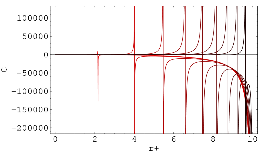
Figure 1: The heat capacity $C_{Q}$ vs. $r_{+}$ of the Kaluza-Klein black hole. Here we have set $r_{\infty}=10$. Different curves correspond to the cases of $r_{-}=0,1,2\cdots 8,9$. The color of the curves changes from red to black when $r_{-}$ increases from $0$ to $9$.

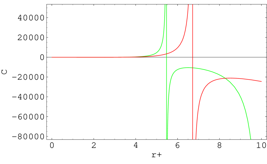
Figure 2: Comparison of the heat capacity $C_{Q}$ vs. $r_{+}$ for Kaluza-Klein black hole and Reissner-Nordström black hole. Here we have set $r_{\infty}=10$, $r_{-}=3$ for the Kaluza-Klein black hole and $r_{\infty}=\infty$, $r_{-}=3$ for the Reissner-Nordström black hole. The red and green curves represent Reissner-Nordström black hole and Kaluza-Klein black hole respectively.

We can consider some limits for the heat capacity of the Kaluza-Klein black hole.

(i). Take the limit $r_{\infty}\rightarrow\infty$, then we have

$$C_{Q}=\frac{3\pi^{2}r_{+}^{3}(r_{+}^{2}-r_{-}^{2})}{2(5r_{-}^{2}-r_{+}^{2})},\quad r_{crit}=\sqrt{5}~{}r_{-}\,.$$ (41)

These are just the heat capacity and critical point of a five-dimensional Reissner-Norström black hole. In the limit, the black hole solution reduces to a five-dimensional Reissner-Nordström black hole.

(ii). When $r_{-}\rightarrow 0$, namely the case without charge, there are no critical points. This case corresponds to a monotonic curve in Fig.1. One can understand this from Eq. (39). In this limit, the heat capacity becomes

$$C_{Q}=\frac{\pi^{2}r_{+}^{3}(r_{+}^{2}-3r_{\infty}^{2})}{2(r_{\infty}^{2}-r_{+}^{2})}$$ (42)

and it further gives the heat capacity of a five-dimensional Schwarzschild black hole when $r_{\infty}\rightarrow\infty$. When $r_{+}=0$, the heat capacity vanishes. This is consistent with the fact that there is no thermodynamic properties for the Gross-Perry-Sorkin monopole [9].

(iii). When $r_{+}=r_{-}$, the heat capacity always vanishes. This corresponds to the case of extremal Kaluza-Klein black holes with vanishing Hawking temperature.

5 Conclusion and Discussion

In this paper, we have calculated the mass of the Kaluza-Klein black hole with squashed horizon by using the counterterm method and generalized Abbott-Deser method. Since the generalized Abbott-Deser method is background dependent, only when a suitable background (13) is chosen, it gives the same mass as the counterterm method. Only this mass has been shown to satisfy the first law of thermodynamics for the Kaluza-Klein black hole. For example, the mass given in (31), which is obtained by choosing the solution (10) with $\rho_{\pm}=0$ but keeping $\rho_{0}$ finite as the reference background, does not satisfy the first law. Further, we have noticed that the electric potential entering into the first law of the black hole thermodynamic is the potential difference between the black hole horizon and infinity. If without the second term in (7), the potential does not vanish at infinity ($r=r_{\infty})$; this is quite different from the case of Reissner-Nordström black hole solution. In (7) we have taken a gauge so that the electric potential vanishes at infinity. In addition, we have discussed some thermodynamic properties of the Kaluza-Klein black holes, and some interesting limits have been found.

References

- [1] S. W. Hawking, Commun. Math. Phys. 25, 152 (1972).
- [2] R. Emparan and H. S. Reall, Phys. Rev. Lett. 88, 101101 (2002) [arXiv:hep-th/0110260].
- [3] H. Ishihara and K. Matsuno, arXiv:hep-th/0510094.
- [4] L. F. Abbott and S. Deser, Nucl. Phys. B 195, 76 (1982)
- [5] G. W. Gibbons and S. W. Hawking, Phys. Rev. D 15, 2752 (1977)
- [6] J. D. Brown and J. W. York, Phys. Rev. D 47, 1407 (1993)
- [7] V. Balasubramanian and P. Kraus, Commun. Math. Phys. 208, 413 (1999) [arXiv:hep-th/9902121].
- [8] P. Kraus, F. Larsen and R. Siebelink, Nucl. Phys. B 563, 259 (1999) [arXiv:hep-th/9906127].
- [9] R. B. Mann and C. Stelea, arXive:hep-th/0511180.
- [10] D. Astefanesei and E. Radu, Phys. Rev. D 73, 044014 (2006) [arXiv:hep-th/0509144].
- [11] B. Kleihaus, J. Kunz and E. Radu, arXiv:hep-th/0603119.
- [12] W. Chen, H. Lü and C. N. Pope, arXive:hep-th/0510081.
- [13] H. Cebeci, O. Sarioglu and B. Tekin, Phys. Rev. D 73, 064020 (2006) [arXiv:hep-th/0602117].
- [14] R. M. Wald, Phys. Rev. D 48, 3427 (1993) [arXiv:gr-qc/9307038].
- [15] P. C. W. Davies, Proc. Roy. Soc. Lond. A 353, 499 (1977).