Matter localization and resonant deconfinement in a two-sheeted spacetime

Abstract

In recent papers, a model of a two-sheeted spacetime $M_{4}\times Z_{2}$ was introduced and the quantum dynamics of massive fermions was studied in this framework. In the present study, we show that the physical predictions of the model are perfectly consistent with observations and most important, it can solve the puzzling problem of the four-dimensional localization of the fermion species in multidimensional spacetimes. It is demonstrated that fermion localization on the sheets arises from the combination of the discrete bulk structure and environmental interactions. The mechanism described in this paper can be seen as an alternative to the domain wall localization arising in continuous five dimensional spacetimes. Although tightly constrained, motions between the sheets are, however, not completely prohibited. As an illustration, a resonant mechanism through which fermion oscillations between the sheets might occur is described.

I Introduction

Extradimensions are the backbone of present theoretical physics. During the last years, there has been a considerable interest in Kaluza-Klein like scenarios suggesting that our usual spacetime could be just a slice of a larger dimensional manifold. Recent advances in string theory have thus postulated the existence of ”braneworlds” ($3$-hyperdimensional surfaces embedded in a $N>4$ dimensional manifold) in which we are living on [1,2]. Several issues like the hierarchy between the electroweak and the Planck scales [3,4] as well as the idea that the post-inflationary epoch of our universe was preceded by the collision of D3-branes [5], for instance, have been successfully addressed in such multidimensional approaches.
In braneworld models, it is generally assumed that the standard model particles can not freely propagate into unseen dimensions and must be constrained to live on a $3+1$ submanifold [1,2]. Such conservative point of view adopts the idea that no interaction (except gravitation) can propagate into the bulk or between adjacent branes [6,7,8]. The problem is then to find a physically reasonable mechanism that could effectively constrain the particles to stay confined in a lower dimensional spacetime sheet [1,2,9-20]. In some string theory inspired models, the confinement arises as a natural consequence of the fact that particles are open strings whose endpoints are attached on Dp-branes [1,2]. Other approaches postulate the existence of domain walls in which standard model particles could be entrapped [9-20]. Among earlier works [9,10,11], Rubakov and Shaposhnikov [10] suggested long time ago that the wave function of fermion zero modes could concentrate near domain walls, generating 4D massless chiral fermions attached to them. This idea has attracted much interest over the last years as it can solve in a very elegant way the hierarchy problem [3,4] and the proton decay problem : the extradimensional separation between chiral fermions generates exponentially suppressed couplings between them [21-23]. Nevertheless, most of these scenarios suffer from a significant drawback as they require the existence of external non-gravitational forces like scalar fields. Since the existence of such fields is still the subject of debate [24], the credibility of these scenarios can be reasonably questioned.
In parallel, some attempts have tried to extend the hypothetical graviton capability of moving through the bulk [1,6,7,8] to the case of massive particles as well [12,15,16]. As a result, there could be a possibility for highly massive or energetic particles to acquire a non zero extradimensional momentum and escape from the branes to propagate into the bulk.
Considering these two opposite approaches, it is clear that the question of whether standard model particles are totally or only partially confined on 4D hypersurfaces is still an open issue.
Furthermore, all those approaches perpetuate the tradition inherited from relativity by assuming that the whole universe behaves like a smooth continuum. However, there have been some recent attempts to develop models where the continuous extra dimensions are substituted by discrete dimensions [25-29]. In those approaches, the extra-dimensions are replaced by a finite number of points and the whole universe can be seen as made up of a collection of 4D sheets. Besides keeping the physical richness of multidimensional spacetimes, such multi-sheeted approaches provide also a nice framework where the standard model may arise from pure geometry [25]. In recent works, at the crossroad between brane models and non commutative two-sheeted spacetimes, present authors have studied the quantum dynamics of fermions in a $M_{4}\times Z_{2}$ universe [30-32]. Such a model can be seen as a formal extension of the Kaluza-Klein spacetime with a fifth extradimension restricted to only two points. It was emphasised that despite the discrete bulk structure, both spacetime sheets are still connected at the quantum level. This connection was shown to be related to the specific geometrical structure of the bulk with a coupling strength partly dictated by the magnitude of the electromagnetic gauge fields of both sheets.
In this paper, we propose to discuss the predictions of our model for the issue concerning the fermion localization on the 4D sub-manifolds. In section 2 we briefly summarize the mathematics underlying our approach and the main results of previous works are reported. In section 3, we detail the mechanisms by which fermions are effectively confined on the 4D sheets. It is demonstrated that the confining effect arises from the combination of the discrete bulk structure and the environmental interactions. To the authors knowledge, the mechanism described here is completely new and presents the advantage of not relying neither on any exotic trapping mechanism involving negative bulk energy nor on any scalar fields.
Besides, in section 4, we show that particles can have access granted to the other spacetime sheet in some specific circumstances. This situation which is analogous to a motion through the bulk in braneworld models is illustrated by considering a resonant mechanism forcing the particle to oscillate between the two sheets. This mechanism which might be experimentally investigated at present times and energy scales is worth being studied as it could become a practical tool for the experimental search of extradimensions.

II Physical and mathematical framework

In Refs. [30-32], a model aiming at describing the quantum dynamics of fermions in a two-sheeted spacetime was described. It corresponds formally to the product of a four continuous manifold times a discrete two points space, i.e. $X=M_{4}\times Z_{2}$.
Such a universe can be pictured as a five dimensional universe where the fifth dimension is replaced by a discrete two points space with coordinates $\pm\delta/2$. Each point is then endowed with its own four-dimensional sheet and both sheets are separated by a distance $\delta$. At that point, it is important to stress that this distance is just a phenomenological one and does not necessarily match the concept of distance we are familiar with. The interaction between both sheets is reflected by the existence of a coupling strength $g=1/\delta$ (see figure 1) given by the inverse distance between the sheets. In the abovementioned references, it was demonstrated that the model could be built by considering two different approaches which are now briefly described.

 

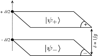
Figure 1: Naive view of the two-sheeted spacetime under consideration. The coupling constant $g$ between the sheets is related to the distance which separates them in the extra-space.

The first approach was mainly based on the work of Connes [25], Viet and Wali [26,27] and relies on a non-commutative definition of the exterior derivative acting on the product manifold. Due to the specific geometrical structure of the bulk, this operator is given by

$$D_{\mu}=\left({{\ \begin{array}[]{cc}{\partial_{\mu}}&0\\ 0&{\partial_{\mu}}\end{array}}}\right),\text{ }\mu=0,1,2,3\text{ and\ }D_{5}=\left({{\ \begin{array}[]{cc}0&g\\ {-g}&0\end{array}}}\right)$$ (1)

Where the term $g$ has the dimension of mass (in $\hbar=c=1$ units) and acts as a finite difference operator along the discrete dimension. In the model discussed in Ref. [30] and contrary to previous works, $g$ was considered as a constant geometrical field (and not the Higgs field [25]). As a consequence a mass term was introduced and a two-sheeted Dirac equation was derived

$$\left({iD\!\!\!/-M}\right)\Psi=\left({i\Gamma^{N}D_{N}-M}\right)\Psi=\left({{\ \begin{array}[]{cc}{i\gamma^{\mu}\partial_{\mu}-m}&{ig\gamma^{5}}\\ {ig\gamma^{5}}&{i\gamma^{\mu}\partial_{\mu}-m}\end{array}}}\right)\left({{\ \begin{array}[]{c}{\psi_{+}}\\ {\psi_{-}}\end{array}}}\right)=0$$ (6)

It can be noticed that by virtue of the two-sheeted structure of spacetime, the wave function $\psi$ of the fermion is split into two components, each component living on a distinct spacetime sheet. Obviously, the equation (2) can also be derived from the $M_{4}\times Z_{2}$ lagrangian L defined as

$$\textsl{L}=\bar{\Psi}\left({i\not{D}-M}\right)\Psi$$ (7)

Where $\bar{\Psi}=\left({\bar{\psi}_{+},\bar{\psi}_{-}}\right)$ is the two-sheeted adjoint spinor of $\Psi$ and with $\bar{\psi}_{+}$ and $\bar{\psi}_{-}$ the adjoint spinors respectively of $\psi_{+}$ and $\psi_{-}$. Such a lagrangian can be also written using the following expended form

L $$= \bar{\psi}_{+}\left({i\not{\partial}-m}\right)\psi_{+}+\bar{\psi}_{-}\left({i\not{\partial}-m}\right)\psi_{-}+ig\bar{\psi}_{+}\gamma^{5}\psi_{-}+ig\bar{\psi}_{-}\gamma^{5}\psi_{+}$$ (8)

At first sight, the doubling of the wave function can be seen as a reminiscence of the hidden-sector concept. While it is true that hidden sector models and present approach share several common points, it is equally true that they differ by the number of spacetime sheets they consider. For instance, the so-called mirror matter approach, considers only one 4D manifold and justifies for the left/right parity by introducing new internal degrees of freedom to particles (see for instance Ref. [33]). In the present work, it can be noticed that the number of particle families remains unchanged but the particles, thanks to their five dimensional nature, have access granted to the two 4D sheets. So, instead of considering new internal degrees of freedom, we simply allow the particles to move freely in an extended spacetime.
The second approach developed in Ref. [31] started from the usual covariant Dirac equation in 5D. By assuming a discrete structure of the bulk, with two four-dimensional submanifolds, the extradimensional derivative has to be replaced by a finite difference counterpart

$$(\partial_{5}\psi)_{\pm}=\pm g(\psi_{+}-\psi_{-})$$ (9)

Then, as in the non-commutative approach, the Dirac equation breaks down into a set of two coupled differential equations similar to Eq. (2) [31].
The incorporation of the electromagnetic field in the model can be done quite easily [30-32]. The usual U(1) gauge field must be substituted by an extended U(1)$\bigotimes$U(1) gauge relevant for the discrete $Z_{2}$ structure of the universe. In addition, each sheet possesses its own current and charge density distribution as source of the electromagnetic field. The most general form for the new gauge (to be incorporated within the two-sheeted Dirac equation such that $D\!\!\!/\rightarrow D\!\!\!/+A\!\!\!/$) is then defined by (see also Refs. [28] and [29] where such a gauge was also considered)

$$A\!\!\!/=\left({{\ \begin{array}[]{cc}{iq\gamma^{\mu}A_{+,\mu}}&{\gamma^{5}\chi}\\ {\gamma^{5}\chi^{\dagger}}&{iq\gamma^{\mu}A_{-,\mu}}\end{array}}}\right)$$ (10)

On the two sheets live then the distinct $\mathbf{A}_{+}$ and $\mathbf{A}_{-}$ fields. In the present model, the component $\chi$ cannot be associated with the usual Higgs field encountered in GSW model. $\chi$ is the coupling of the photons fields of the two sheets. Since this term introduces obvious complications unless to be weak enough compared to $\mathbf{A}_{\pm}$ (most notably it leads to unusual transformations laws of the electromagnetic field which are difficult to reconcile with observations) it is preferable to set $\chi=0$. The electromagnetic fields of both sheets are then completely decoupled and each sheet is endowed with its own electromagnetic structure. Note that the consequence of having $\chi\neq 0$ would have been to couple each charged particle with the electromagnetic field of both sheets, irrespective of the localization of this particle in the bulk. For instance a particle of charge $q$ localized in the sheet $(+)$ would have been sensitive to the electromagnetic field of the sheet $(-)$ with an effective charge $\varepsilon q$ ($\varepsilon<1$). This kind of exotic interactions has been considered previously in literature within the framework of the mirror matter paradigm and is not covered by the present paper [34,35]. Another relevant consequence of considering $\chi=0$ is that the photons fields are now totally trapped in their original sheets : photons belonging to a given sheet are not able to go into the other sheet (as a noticeable consequence, the structures belonging to a given sheet are invisible from the perspective of an observer located in the other sheet). The classical gauge field transformation which reads

$$A_{\mu}^{\prime}=A_{\mu}+\partial_{\mu}\Lambda$$ (11)

can be easily extended to fulfil the two-sheeted requirements. A solution consistent with the above hypothesis $\chi=0$ shows that the gauge transformation is degenerated and reduced to a single $e^{iq\Lambda}$ which must be applied to both sheets simultaneously [30,31]. By setting $\chi=0$ and by considering the same gauge transformation in the two sheets we can get photons fields $\mathbf{A}_{\pm}$ which behave independently from each other and in accordance with observations [30-32]. After introducing the gauge field into the $Z_{2}$ Dirac equation and taking the non relativistic limit (following the standard procedure), a two-sheeted Pauli like equation can be derived [30-32] (using now natural units)

$$i\hbar\frac{\partial}{\partial t}\left(\begin{array}[]{c}\left|\psi_{+}\right\rangle\\ \left|\psi_{-}\right\rangle\end{array}\right)=\left\{\mathbf{H}+\mathbf{H}_{cm}(g,\mathbf{A}_{\pm})+\mathbf{H}_{c}(g^{2})\right\}\left(\begin{array}[]{c}\left|\psi_{+}\right\rangle\\ \left|\psi_{-}\right\rangle\end{array}\right)$$ (12)

where $\left|\psi_{+}\right\rangle$ and $\left|\psi_{-}\right\rangle$ correspond to the wave functions in the $(+)$ and $(-)$ sheets respectively. The Hamiltonian $\mathbf{H}$ is a block-diagonal matrix where each block is simply the classical Pauli Hamiltonian expressed in both sheets

$$\mathbf{H}_{\pm}=-\frac{\hbar^{2}}{2m}\left(\mathbf{\nabla}-i\frac{q}{\hbar}\mathbf{A}_{\pm}\right)^{2}+g_{s}\mu\frac{1}{2}\mathbf{\sigma\cdot B}_{\pm}+V_{\pm}$$ (13)

and such that $\mathbf{A}_{+}$ and $\mathbf{A}_{-}$ denote the magnetic vector potentials in the sheet $(+)$ and $(-)$ respectively. The same convention is applied for the magnetic fields $\mathbf{B}_{\pm}$. $g_{s}\mu$ is the magnetic moment of the particle with $g_{s}$ the gyromagnetic factor and $\mu$ the magneton. In addition to these “classical” terms, the two-sheeted Hamiltonian comprises also new terms involving the discrete structure of the bulk. $\mathbf{H}_{c}$ is a constant geometrical term proportional to the square of the coupling constant $g^{2}$ and $\mathbf{H}_{cm}$ is another geometrical coupling involving the gauge fields of the two sheets. This last term is proportional to $g$. Since $g^{2}$ must be tiny in order for the model to be consistent with the experimental observations and measurements, the term $\mathbf{H}_{c}$ can be neglected in a first approximation [30-32]. As a consequence, $\mathbf{H}_{cm}$ imparts most of the new physics of the model. This contribution takes the form [30-32]

$$\mathbf{H}_{cm}=-ig\gamma g_{s}\mu\frac{1}{2}\left[\begin{array}[]{cc}0&\mathbf{\sigma\cdot}\left\{\mathbf{A}_{+}-\mathbf{A}_{-}\right\}\\ -\mathbf{\sigma\cdot}\left\{\mathbf{A}_{+}-\mathbf{A}_{-}\right\}&0\end{array}\right]$$ (14)

As a consequence, the remaining coupling term $\mathbf{H}_{cm}$ arises through the magnetic vector potentials $\mathbf{A}_{+}$ and $\mathbf{A}_{-}$ and the magnetic moment $g_{s}\mu$. In Eq. (10), $\gamma$ is a constant and $g_{c}=\gamma g_{s}$ stands for the isogyromagnetic factor [31]. From a theoretical point of view, the neglect of the QED corrections leads to $g_{s}=g_{c}=2$ for an electron [31]. As a consequence $\gamma$ must be equal to $1$. Although it was suggested in Ref. [31] that $g_{c}$ could differ slightly from $g_{s}$ when taking into account QED, these corrections will not be considered in the present paper. As a consequence, in the proton or neutron cases, we consider also $\gamma=1$ and use the standard experimental values of $g_{s}$ (i.e. 5.58 and -3.82 respectively) [31]. It is worth being noticed that $g\left\{\mathbf{A}_{+}-\mathbf{A}_{-}\right\}$ can be seen as an extradimensional magnetic field. The similarities between $\mathbf{H}_{cm}$ and the classical term $g_{s}\mu(1/2)\mathbf{\sigma\cdot B}_{\pm}$ become more obvious when considering the presence of the magnetic moment in Eq. (10).

III Dynamics of the particles localization

The coupling term $\mathbf{H}_{cm}$ arises from the geometrical proximity between the two sheets. As a consequence, even if these sheets do not share any 4D link, the particles can possibly move from one sheet to the other one. Such a delocalization between the two sheets can be seen as a major drawback of the model but we are now going to show that environmental interactions constrain the capability of moving between the sheets. An illustrative example can be given. Let us consider a fermion moving in a constant magnetic vector potential $\mathbf{A}_{+}=A\mathbf{e}_{z}$ created in the first sheet. Assuming that $\mathbf{H}$ can be expressed in its diagonal form, the particle dynamics reduces to

$$i\hbar\frac{\partial}{\partial t}\left|\Psi(t)\right\rangle=\left\{\left[\begin{array}[]{cc}E_{+}&0\\ 0&E_{-}\end{array}\right]\mathbf{+}i\hbar\Omega\left[\begin{array}[]{cc}0&-\sigma_{z}\\ \sigma_{z}&0\end{array}\right]\right\}\left|\Psi(t)\right\rangle$$ (15)

where $\Omega=gg_{s}\mu A/(2\hbar)$. Provided that the particle is originally located in the sheet $(+)$ and unpolarized, it is straightforward to show that the probability to find the particle in the $(-)$ sheet is

$$P=\frac{1}{1+\zeta^{2}}\sin^{2}\left(\Omega\sqrt{1+\zeta^{2}}t\right)$$ (16)

with $\zeta=(E_{+}-E_{-})/(2\Omega\hbar).$ It is worth being noticed that the difference $\Delta E$ between the eigenvalues $E_{+}$ and $E_{-}$ of the Hamiltonian $\mathbf{H}$ plays a fundamental role as it governs the particle ability of reaching the second sheet (i.e. of moving in the discrete space). For that reason, it is convenient to recast it in the following form

$$\Delta\mathbf{H}=\Delta V_{grav}+\Delta V_{elec}+\Delta K_{A}+g_{s}\mu\frac{1}{2}\mathbf{\sigma\cdot}\Delta\mathbf{B}$$ (17)

with

$$K_{A,\pm}=-\frac{q}{m}\mathbf{A}_{\pm}\cdot\widehat{\mathbf{P}}+\frac{q^{2}}{2m}\left|\mathbf{A}_{\pm}\right|^{2}$$ (18)

In Eq. (13), the gravitational and electrostatic contributions have been included in the potential in order to give $\Delta\mathbf{H}$ the most general form.
In the following, we restrict ourselves to the case of an irrotational magnetic vector potential such that $\mathbf{B=0}$. From Eq. (12), it is then clear that if $\zeta=0$, i.e. $\Delta E=E_{+}-E_{-}=0$, the particle oscillates freely between the two sheets with a time periodicity $T=2\pi\hbar/(gg_{s}\mu A)$. Note that during the oscillations, the particle which is a $M_{4}\times Z_{2}$ entity, behaves sometimes as a four dimensional $M_{4}$ one. Indeed, when the maximum of the probability is reached (i.e. 1), the particle becomes totally localized in a four dimensional submanifold. From this point of view, it is clear that the particle is not spontaneaously constrained to stay on a specific sheet. Such ability to move between the sheets, can be seen as a discrete counterpart of motions in the bulk sometimes discussed in brane-world models.
Although the particles are able to oscillate between the sheets, four dimensional localization can still occur in this model. We start by considering $\zeta\neq 0$ i.e. there is now an effective potential $\Delta\mathbf{H}$ applied onto the particle. Then, it is trivial to see that the amplitude and the period of oscillations change. The higher the potential is, the weaker the oscillation amplitude is. Therefore, in presence of a strong enough potential, the particle is now confined on its sheet and cannot reach the other one. Since, the potential is in fact the sum of all external influences acting on the particle, it becomes obvious that the confinement arises mainly from environmental interactions. Such an explanation of the matter confinement in a multidimensional spacetime is elegant in several aspects: first, it does not require any ad-hoc bulk field nor any extradimensional gravitational trapping mechanism [9-23]. Secondly, it is quite remarkable that the model suggests that the confinement of fermions may arise from usual 4D interactions (particle scattering, EM interactions, gravitational fields…).
Note that the matter confinement could perhaps be insured even for large value of $g$ provided that the intensity of the environmental interactions are significant.
Let us consider more closely the electrostatic and gravitational contributions in $\Delta E$. With regards to the electrostatic potentials, the neutrality of matter implies that they can be neglected at our scale or any larger scale. At smaller scale however, as inside an atom for instance, the typical potential energies undergone by an electron are about $-10$ eV, which is a quite small value. The same cannot be said for the gravitational potentials. We consider the typical example of a single neutron interacting with a larger object like the earth, the sun or the Milky Way core (which is responsible for the sun attraction around the galactic center). If the acceleration induced by the earth on a neutron is $a=1$, then it is $a=6\times 10^{-4}$ and $a=2\times 10^{-11}$ for the sun and the Milky Way core respectively. Although the gravitational forces exerted by a very distant object can be neglected, the gravitational potentials can become huge as we can convince oneself easily. For a neutron in the lab reference frame, the potential energy arising from the earth/particle interaction is $0.65$ eV (absolute value), this potential reaches $9$ eV when considering the sun influence and it rises up to $500$ eV for the Milky Way core. Although the induced acceleration by such a massive object is negligible in an earth lab, its effect on the potential energy of particles is considerable. It is of course related to the fact that the gravitational potential varies like $1/r$ and the force like $1/r^{2}$ with $r$ the distance between the particle and the influencing massive object. In such circumstances, it appears that the main contribution to the confinement is the gravitational potential exerted by massive objects or clusters of matter. Until now we have only discussed the gravitational contribution of the mass located in our sheet but from Eq. (13), it is clear that the masses located in the neighboring sheet also constrain the particle oscillations. Unfortunately, to assess the gravitational influence of the masses located in the other sheet, we need some kind of gravitational telescope which does not exist at present time.
Let us now calculate the effective probability for a single particle, to oscillate between the two sheets. We are going to assume a coupling constant of the order $g=10^{-1}$ m^-1 (which is a quite huge value). Typically, the magnetic potential can be related to a current intensity $I$ through $A=\mu_{0}I$ ($\mu_{0}$ is the vacuum permeability). Therefore, intensity can be considered as a good indicator of the reachable magnetic potentials. We thus consider an intensity of $10^{9}$ A and a global confining potential of $500$ eV. For a neutron, the Eq. (12) indicates that the maximum amplitude of the oscillations of probability is $2.5\cdot 10^{-16}$. This value is so tiny that it is hard to believe that any particle oscillations might be observed in the physical world. Hence, in all practical cases, the confining effect is so strong that the particles are constrained to move on their sheet only. Such a result is interesting because it shows that the model does not violate any current observations. However, it is unsatisfactory because it seems to prohibit any attempt to confirm the existence of a coupling between the neighboring sheets as predicted by this model. A closer investigation of $\mathbf{H}_{cm}$ suggests however a way to enhance the probability amplitude.

IV Resonant leap between spacetime sheets

Obviously, a first way to enhance the probability of oscillations is to increase the intensity of the vector potential and/or to decrease the gravitational trapping potential. Unfortunately, since gravity cannot be shielded and since magnetic potential is limited by the reachable current intensity, these solutions remain poorly effective. Previously, the similarity between $\mathbf{H}_{cm}$ and the term $g_{s}\mu(1/2)\mathbf{\sigma\cdot B}_{\pm}$ was noted. Since this last term is traditionally involved in magnetic resonance, it is legitimate to search for a two-sheeted counterpart of this mechanism through which particle oscillations might occur. Let us again consider the two-sheeted Pauli equation (Eq. (8)). By analogy with magnetic resonance, we are now going to consider a particle initially located in the first sheet and subjected to a rotating curl-free magnetic vector potential. The irrotational character of the magnetic potential precludes the existence of a related magnetic field and thus prevents the existence of a Hamiltonian contribution of the form $g_{s}\mu(1/2)\mathbf{\sigma\cdot B}$. Let us choose $\mathbf{A}_{+}=\mathbf{A}_{p}=A_{p}\mathbf{e(}t\mathbf{)}$ and $\mathbf{A}_{-}=\mathbf{0}$ with the magnetic vector potential rotating in the $Oxy$ plane, i.e.

$$\mathbf{e(}t\mathbf{)=}\left[\begin{array}[]{c}\cos\omega t\\ \sin\omega t\\ 0\end{array}\right]$$ (19)

For simplicity reasons, it is assumed that $\mathbf{H}$ can be expressed in its diagonal form. The eigenstates of the Hamiltonian $\mathbf{H}$ are defined as

$$\left|\psi_{+1/2}^{+}\right\rangle=\left[\begin{array}[]{c}1\\ 0\\ 0\\ 0\end{array}\right]\text{, }\left|\psi_{-1/2}^{+}\right\rangle=\left[\begin{array}[]{c}0\\ 1\\ 0\\ 0\end{array}\right]$$ (20)

for particles located in the first sheet with an energy equals to $E_{+}$ (assuming both spin states $\pm 1/2$), and

$$\left|\psi_{+1/2}^{-}\right\rangle=\left[\begin{array}[]{c}0\\ 0\\ 1\\ 0\end{array}\right]\text{, }\left|\psi_{-1/2}^{-}\right\rangle=\left[\begin{array}[]{c}0\\ 0\\ 0\\ 1\end{array}\right]$$ (21)

for particles located in the second sheet with an energy equals to $E_{-}$ (assuming both spin states $\pm 1/2$). Taking into account these assumptions, Eq. (8) becomes

$$i\hbar\frac{\partial}{\partial t}\left|\Psi(t)\right\rangle = \left\{\left[\begin{array}[]{cc}E_{+}&0\\ 0&E_{-}\end{array}\right]+i\Omega_{p}\hbar\left[\begin{array}[]{cc}0&-\mathbf{\sigma\cdot e}\\ \mathbf{\sigma\cdot e}&0\end{array}\right]\right\}\left|\Psi(t)\right\rangle$$ (26)

with $\Omega_{p}=g\gamma g_{s}\mu A_{p}/(2\hbar)=E_{p}/\hbar$. It is then possible to develop the general solution as

$$\left|\Psi(t)\right\rangle = a(t)\left|\psi_{+1/2}^{+}\right\rangle e^{-i(1/\hbar)E_{+}t}+b(t)\left|\psi_{-1/2}^{+}\right\rangle e^{-i(1/\hbar)E_{+}t}$$ (27)

$${}+c(t)\left|\psi_{+1/2}^{-}\right\rangle e^{-i(1/\hbar)E_{-}t}+d(t)\left|\psi_{-1/2}^{-}\right\rangle e^{-i(1/\hbar)E_{-}t}$$

This solution can be inserted into Eq. (18) to give the following system

$$\left\{\begin{array}[]{c}\frac{d}{dt}a(t)=-\Omega_{p}d(t)e^{i(\eta-\omega)t}\\ \frac{d}{dt}b(t)=-\Omega_{p}c(t)e^{i(\eta+\omega)t}\\ \frac{d}{dt}c(t)=\Omega_{p}b(t)e^{-i(\eta+\omega)t}\\ \frac{d}{dt}d(t)=\Omega_{p}a(t)e^{-i(\eta-\omega)t}\end{array}\right.$$ (32)

where $\eta=(E_{+}-E_{-})/\hbar$. This system can be trivially solved by analytical means. Using the initial conditions $a(t=0)=a_{0}$, $b(t=0)=b_{0}$ and $c(t=0)=d(t=0)=0$ with $\left|a_{0}\right|^{2}+\left|b_{0}\right|^{2}=1$ (i.e. the particle is initially localized in the $(+)$ sheet), one obtains

$$a(t) = a_{0}\biggl{\{}\cos\left((1/2)\sqrt{(\eta-\omega)^{2}+4\Omega_{p}^{2}}t\right)$$

$$-i\frac{\eta-\omega}{\sqrt{(\eta-\omega)^{2}+4\Omega_{p}^{2}}}\sin\left((1/2)\sqrt{(\eta-\omega)^{2}+4\Omega_{p}^{2}}t\right)\biggr{\}}e^{i(1/2)(\eta-\omega)t}$$

$$b(t) = b_{0}\biggl{\{}\cos\left((1/2)\sqrt{(\eta+\omega)^{2}+4\Omega_{p}^{2}}t\right)$$

$$-i\frac{\eta+\omega}{\sqrt{(\eta+\omega)^{2}+4\Omega_{p}^{2}}}\sin\left((1/2)\sqrt{(\eta+\omega)^{2}+4\Omega_{p}^{2}}t\right)\biggr{\}}e^{i(1/2)(\eta+\omega)t}$$

$$c(t) = -b_{0}\frac{2\Omega_{p}}{\sqrt{(\eta+\omega)^{2}+4\Omega_{p}^{2}}}\sin\left((1/2)\sqrt{(\eta+\omega)^{2}+4\Omega_{p}^{2}}t\right)e^{-i(1/2)(\eta+\omega)t}$$ (35)

$$d(t) = -a_{0}\frac{2\Omega_{p}}{\sqrt{(\eta-\omega)^{2}+4\Omega_{p}^{2}}}\sin\left((1/2)\sqrt{(\eta-\omega)^{2}+4\Omega_{p}^{2}}t\right)e^{-i(1/2)(\eta-\omega)t}$$ (36)

If the spin was in the $+1/2$ state at $t=0$ ($a_{0}=1$ and $b_{0}=0$), it can then be shown using Eq. (24) that the probability $P$ to find the particle in the second sheet is given by

$$P=\frac{4\Omega_{p}^{2}}{(\eta-\omega)^{2}+4\Omega_{p}^{2}}\sin^{2}\left((1/2)\sqrt{(\eta-\omega)^{2}+4\Omega_{p}^{2}}t\right)$$ (37)

and in addition, the particle is then in the down spin state. By contrast, if the spin was in the $-1/2$ state at $t=0$ we get for the probability $P$

$$P=\frac{4\Omega_{p}^{2}}{(\eta+\omega)^{2}+4\Omega_{p}^{2}}\sin^{2}\left((1/2)\sqrt{(\eta+\omega)^{2}+4\Omega_{p}^{2}}t\right)$$ (38)

and now the particle is in the spin up state in the second sheet. Eq. (25) corresponds to a resonant process : as the potential vector rotates with the angular frequency $\omega=\eta$ the probability $P$ presents a maximal amplitude equals to one, independently of the coupling constant and of the magnetic vector potential amplitude. In addition, the probability oscillates with an angular frequency given by $\Omega_{p}$. The resonance width at the half-height is $\Delta\omega=4\Omega_{p}$. The weaker the coupling constant $g$ is, the narrower the resonance is. By contrast, the greater the magnetic vector potential $A_{p}$ is, the broader the resonance is. Note that Eq. (26) is similar to Eq. (25) except that it describes an anti-resonance associated with a counter-rotating vector potential. Both Eq. (25) and (26) remind those found in magnetic resonance (MR) where the spin orientation is influenced by the combination of a static and an oscillating magnetic field. In the present case, the matter exchange between the sheets arises from the resonant interaction between the rotating curl-free magnetic vector potential and the spin (via the magnetic moment). Note that the diagonal contribution of the Hamiltonian in Eq. (18) plays a role similar to the spin/static magnetic field interaction found in MR. But if $E_{+}-E_{-}$ stands for the difference of magnetic energy between two spin states in MR, the difference $\Delta E$ in our model arises from a completely different origin. As a consequence, when the angular frequency $\omega$ of the magnetic vector potential matches the confinement potential $\Delta E/\hbar$ (see previous section) the particle is resonantly transferred from one sheet to the other one. In practice, any rotating vector potential induces electric field and possibly magnetic field that can skew dramatically any experimental study by increasing the contribution of $\Delta E$. Even if we work with a neutral particle (a neutron for instance), the use of an irrotational magnetic vector potential is necessary to avoid any undesirable magnetic field. This requirement may be difficult to fulfill and an electromagnetic wave is not necessarily relevant for this purpose. Therefore, obtaining the required conditions for a resonant transfer remains a major challenge although it could perhaps be accessible with our current technology.

V Conclusion

In this paper, the quantum behavior of massive particles has been studied within the framework of the two-sheeted spacetime model introduced in earlier works. The model predicts that fermions oscillate between the two spacetime sheets in presence of irrotational vector potentials. It is shown however that environmental interactions constrain very tightly these oscillations and lead to a four-dimensional localization of the fermion species. Yet, we predict that the environmental confining effect can be overcome through a resonant mechanism which might be investigated at a laboratory scale. The study of such a mechanism could be relevant for demonstrating the existence of another spacetime sheet and confirms that our spacetime is just a sheet embedded in a more complex manifold.

References

- (1) P. Horava, E. Witten, “Heterotic and Type I String Dynamics from Eleven Dimensions”, Nucl. Phys. B460 (1996) 506-524 (hep-th/9510209)
- (2) A. Lukas, B.A. Ovrut, K.S. Stelle, D. Waldram, “The Universe as a Domain Wall”, Phys. Rev. D59 (1999) 086001 (hep-th/9803235)
- (3) L. Randall, R. Sundrum, “Large mass hierarchy from a small extra dimension”, Phys. Rev. Lett. 83, 3370 (1999) (hep-ph/9905221)
- (4) N. Arkani-Hamed, L. Hall, D. Smith, N. Weiner, “Solving the Hierarchy Problem with Exponentially Large Dimensions”, Phys. Rev. D62 (2000) 105002 (hep-ph/9912453)
- (5) J. Khoury, B.A. Ovrut, P.J. Steinhardt, N. Turok , “The Ekpyrotic Universe: Colliding Branes and the Origin of the Hot Big Bang”, Phys. Rev. D64 (2001) 123522 (hep-th/0103239)
- (6) L. Randall, R. Sundrum, “An alternative to compactification”, Phys. Rev. Lett. 83, 4690 (1999) (hep-th/9906064)
- (7) N. Arkani-Hamed, S. Dimopoulos, G. Dvali, N. Kaloper, “Manyfold Universe”, JHEP 0012, 010 (2000) (hep-ph/9911386)
- (8) A. Barvinsky, A. Kamenshchik, C. Kiefer, A. Rathke, “Graviton oscillations in the two-brane world”, Phys. Lett. B571 (2003) 229-234 (hep-th/0212015)
- (9) K. Akama, “Pregeometry”, Lect. Notes in Phys. 176, 267 (1983) (hep-th/0001113)
- (10) V.A. Rubakov, M.E. Shaposhnikov, “Do we live inside a domain wall?”, Phys. Lett. B125 (1983) 136-138
- (11) M. Pavsic, “Einstein’s gravity from a first order lagrangian in an embedding space”, Phys. Lett. A116 (1986) 1-5 (gr-qc/0101075)
- (12) R. Bryan, “Are the Dirac particles of the Standard Model dynamically confined states in a higher-dimensional flat space?”, Can. J. Phys. 77, 197 (1999) (hep-ph/9904218)
- (13) S. Randjbar-Daemi, M. Shaposhnikov, “Fermion zero-modes on brane-worlds”, Phys. Lett. B492 (2000) 361-364 (hep-th/0008079)
- (14) B. Bajc, G. Gabadadze, “Localization of Matter and Cosmological Constant on a Brane in Anti de Sitter Space”, Phys. Lett. B474 (2000) 282-291 (hep-th/9912232)
- (15) R. Gregory, V.A. Rubakov, S.M. Sibiryakov, “Brane worlds: the gravity of escaping matter”, Class. Quant. Grav. 17, 4437 (2000) (hep-th/0003109)
- (16) S.L. Dubovsky, V.A. Rubakov, P.G. Tinyakov, “Brane world: disappearing massive matter”, Phys. Rev. D62, 105011 (2000) (hep-th/0006046)
- (17) M. Pavsic, “A Brane World Model with Intersecting Branes”, Phys. Lett. A283 (2001) 8-14 (hep-th/0006184)
- (18) A. Kehagias, K. Tamvakis, “Localized Gravitons, Gauge Bosons and Chiral Fermions in Smooth Spaces Generated by a Bounce”, Phys. Lett. B504 (2001) 38-46 (hep-th/0010112)
- (19) C. Ringeval, P. Peter, J. P. Uzan, “Localization of massive fermions on the brane”, Phys. Rev. D65 (2002) 044016 (hep-th/0109194)
- (20) A. Melfo, N. Pantoja, J.D. Tempo, “Fermion localization on thick branes”, Phys.Rev. D73 (2006) 044033 (hep-th/0601161)
- (21) G. Altarelli, F. Feruglio, “SU(5) Grand Unification in Extra Dimensions and Proton Decay”, Phys. Lett. B511 (2001) 257-264 (hep-ph/0102301)
- (22) Y. Kawamura, “Triplet-doublet Splitting, Proton Stability and Extra Dimension”, Prog. Theor. Phys. 105 (2001) 999-1006 (hep-ph/0012125)
- (23) N. Arkani-Hamed, Y. Grossman, M. Schmaltz, “Split Fermions in Extra Dimensions and Exponentially Small Cross-Sections at Future Colliders”, Phys. Rev. D61 (2000) 115004 (hep-ph/9909411)
- (24) K. Dimopoulos, “Can a vector field be responsible for the curvature perturbation in the Universe?”, (hep-ph/0607229)
- (25) A. Connes, J. Lott, “Particle models and non-commutative geometry”, Nucl. Phys. B18 (Proc.Suppl.) (1990) 29-47
- (26) N.A. Viet, K.C. Wali, “A Discretized Version of Kaluza-Klein Theory with Torsion and Massive Fields”, Int. J. Modern Phys. A11 (1996) 2403 (hep-th/9508032)
- (27) N.A. Viet, K.C. Wali, “Non-commutative geometry and a Discretized Version of Kaluza-Klein theory with a finite field content”, Int. J. Mod. Phys. A11 (1996) 533 (hep-th/9412220)
- (28) F. Lizzi, G. Mangano, G. Miele, “Another Alternative to Compactification: Noncommutative Geometry and Randall-Sundrum Models”, Mod. Phys. Lett. A16 (2001) 1-8 (hep-th/0009180)
- (29) H. Kase, K. Morita, Y. Okumura, “Lagrangian Formulation of Connes’ Gauge Theory”, Prog. Theor. Phys. 101 (1999) 1093-1103 (hep-th/9812231)
- (30) F. Petit, M. Sarrazin, “Quantum dynamics of massive particles in a non-commutative two-sheeted space-time”, Phys. Lett. B612 (2005) 105-114 (hep-th/0409084)
- (31) M. Sarrazin, F. Petit, “Quantum dynamics of particles in a discrete two-branes world model: Can matter particles exchange occur between branes?”, Acta Phys. Polon. B36 (2005) 1933-1950 (hep-th/0409083)
- (32) M. Sarrazin, F. Petit, “Artificially induced positronium oscillations in a two-sheeted spacetime: consequences on the observed decay processes”, Int. J. Mod. Phys. A21 (2006) 6303-6314 (hep-th/0505014)
- (33) R. Foot, H. Lew, R.R. Volkas, “Unbroken versus broken mirror world: a tale of two vacua”, JHEP 0007 (2000) 032 (hep-ph/0006027)
- (34) R. Foot, A. Yu. Ignatiev, R. R. Volkas, “Physics of mirror photons”, Phys. Lett. B503 (2001) 355-361 (astro-ph/0011156)
- (35) S. Abel, B. Schofield, “Brane-Antibrane Kinetic Mixing, Millicharged Particles and SUSY Breaking”, Nucl. Phys. B685 (2004) 150-170 (hep-th/0311051)