Spinor Casimir effect for concentric spherical shells in the global monopole spacetime

Abstract

In this paper we investigate the vacuum polarization effects associated with a massive fermionic field due to the non-trivial topology of the global monopole spacetime and boundary conditions imposed on this field. Specifically we investigate the vacuum expectation values of the energy-momentum tensor and fermionic condensate admitting that the field obeys the MIT bag boundary condition on two concentric spherical shells. In order to develop this analysis, we use the generalized Abel-Plana summation, which allows to extract from the vacuum expectation values the contribution coming from a single sphere geometry and to present the second sphere induced part in terms of exponentially convergent integrals. In the limit of strong gravitational field corresponding to small values of the parameter describing the solid angle deficit in global monopole geometry, the interference part in the expectation values are exponentially suppressed. The vacuum forces acting on spheres are presented as the sum of self-action and interaction terms. Due to the surface divergences, the first one is divergent and needs additional renormalization, while the second one is finite for all non-zero distances between the spheres. By making use of zeta function renormalization technique, the total Casimir energy is evaluated in the region between two spheres. It is shown that the interaction part of the vacuum energy is negative and the interaction forces between the spheres are attractive. Asymptotic expressions are derived in various limiting cases. As a special case we discuss the fermionic vacuum densities for two spherical shells on background of the Minkowski spacetime.

PACS number(s): 03.70.+k, 04.62.+v, 12.39.Ba

1 Introduction

It is well known that different types of topological objects may have been formed in the early universe after Planck time by the vacuum phase transition [1, 2]. Depending on the topology of the vacuum manifold these are domains walls, strings, monopoles and textures. Among them, cosmic strings and monopoles seem to be the best candidate to be observed.

A global monopole is a spherical heavy object formed in the phase transition of a system composed by a self-coupling scalar field iso-triplet $\varphi^{a}$, whose original global $O(3)$ symmetry is spontaneously broken to $U(1)$. The matter fields play the role of an order parameter which outside the monopole’s core acquires a non-vanishing value. The simplified global monopole was introduced by Sokolov and Starobinsky [3]. The gravitational effects of of the global monopole were considered in Ref. [4], where a solution is presented which describes a global monopole at large radial distances. The gravitational effects produced by this object may be approximated by a solid angle deficit in the (3+1)-dimensional spacetime whose line element is given by

$$ds^{2}=dt^{2}-dr^{2}-\alpha^{2}r^{2}\left(d\theta^{2}+\sin^{2}\theta d\phi^{2}\right)\ .$$ (1)

Here the parameter $\alpha^{2}=1-8\pi G\eta^{2}$ is smaller than unity and depends on the energy scale $\eta$ where the global symmetry is spontaneously broken. The energy-momentum tensor associated with this topological object has a diagonal form and reads: $T_{0}^{0}=T_{1}^{1}=(1-\alpha^{2})/\alpha^{2}r^{2}$ and $T_{2}^{2}=T_{3}^{3}=0$. The spacetime defined by the metric tensor above is not flat: the scalar curvature $R=2(1-\alpha^{2})/\alpha^{2}r^{2}$ and the solid angle is $\Omega=4\pi\alpha^{2}$, smaller than the ordinary one, consequently there is a solid angle deficit given by $\delta\Omega=4\pi(1-\alpha^{2})$. It is of interest to note that the effective metric produced in superfluid ${}^{3}\mathrm{He-A}$ by a monopole is described by the line element (1) with the negative angle deficit, $\alpha>1$, which corresponds to the negative mass of the topological object [5]. The quasiparticles in this model are chiral and massless fermions.

The quantum effects due to the point-like global monopole spacetime on the matter fields have been considered for massless scalar [6] and fermionic [7] fields, respectively (for the heat-kernels on the generalized cone see [8, 9]). In order to develop this analysis, the scalar respectively spinor Green functions in this background have been obtained. The influence of the non-zero temperature on these polarization effects has been considered in [10] for scalar and fermionic fields. Moreover, the calculation of quantum effects on massless scalar field in a higher dimensional global monopole spacetime has also been developed in [11].

Two important ingredients responsible for vacuum polarization effects are the non-trivial geometry of the spacetime itself and boundary conditions obeyed by the matter fields. In this direction, the total Casimir energy associated with massive scalar field inside a spherical region in the global monopole background have been analyzed in Refs. [8, 12] by using the zeta function regularization procedure. Moreover, bosonic Casimir densities induced by a single shell have been calculated in [13] to higher dimensional global monopole spacetime by making use of the generalized Abel-Plana summation formula [14, 15]. More recently, using also this formalism, a similar analysis for spinor fields has been developed in [16]. In these publications two distinct situations were examined: the vacuum averages inside and outside the shell. The generalized Abel-Plana summation formula is a powerful instrument which allows to develop the summation over all discrete modes. By using this formula, all the physical vacuum polarization local quantities can be separated in two contributions: boundary dependent parts and independent ones. The boundary independent contributions are similar to previous results obtained in the literature for scalar and fermionic fields, [6, 7], using different approach. These contributions are divergent and consequently in order to obtain finite and well defined results, one must apply some regularization procedure. The boundary dependent contributions, on the other hand, are finite at any strictly interior or exterior points and do not contain anomalies. Consequently, they do not require any regularization procedure.

Bosonic Casimir densities induced by two concentric spherical shells in the global monopole spacetime have been analyzed in [17]. Here we shall continue in this line of investigation, calculating spinor densities for two concentric spherical shells. In this context, we shall admit that the fermionic field obeys the MIT bag boundary conditions on the spherical shells. Specifically we shall calculate the vacuum expectation value of the energy-momentum tensor and the vacuum interaction forces between two shells. Also the total Casimir energy will be considered.

The Casimir effect associated with fermionic fields in a Minkowski background, was considered in a great number of papers [18, 19, 20, 21, 22, 23, 24, 25] (for reviews and additional references see [26, 27, 28, 29, 30]), considering that the fields obey the MIT bag model condition. As far as we know, the most of the previous studies were focused on global quantities, such as the total vacuum energy and stress on the surface. The density of the fermionic vacuum condensate for a massless spinor field inside the bag was investigated in Ref. [20] (see also [29]). As to the Casimir effect it is of physical interest to calculate not only the total energy but also the local characteristics of the vacuum, such as the energy-momentum tensor and vacuum condensate. In addition to describing the physical structure of the quantum field at a given point, the energy-momentum tensor acts as the source of gravity in the Einstein equations. It therefore plays an important role in modelling a self-consistent dynamics involving the gravitational field [31]. For $\alpha=1$ case, our calculation is a local extension of the previous contributions on the fermionic Casimir effect for a spherical shell.

This paper is organized as follows: In Section 2 we consider the vacuum expectation values of the energy-momentum tensor and the fermionic condensate in the region between two spheres. Section 3 is devoted to the investigation of the vacuum interaction forces between the spheres. In Section 4, by using the zeta function technique, we investigate the total Casimir energy in the region between two spheres as a sum of the zero-point energies of elementary oscillators and various limiting cases are discussed. In Section 5 we present our concluding remarks. In Appendix A by using the generalized Abel-Plana formula we derive a summation formula for the series over the eigenmodes of the fermionic vacuum in the region between two spheres.

2 Vacuum expectation values of the energy-momentum tensor and the fermionic condensate

In this section we shall consider a massive spinor field propagating on a point-like global monopole background described by the line element (1). The dynamics of the field is described by the Dirac equation

$$i\gamma^{\mu}(\partial_{\mu}+\Gamma_{\mu})\psi-M\psi=0\ ,$$ (2)

where $\gamma^{\mu}$ are the Dirac matrices defined in such curved spacetime, and $\Gamma_{\mu}=\gamma_{\nu}\nabla_{\mu}\gamma^{\nu}/4$ is the spin connection with $\nabla_{\mu}$ being the standard covariant derivative operator. Here we shall adopt the following representation for the Dirac matrices

$$\gamma^{0}=\left(\begin{array}[]{cc}1&0\\ 0&-1\end{array}\right)\ ,\ \gamma^{k}=\left(\begin{array}[]{cc}0&\sigma^{k}\\ -\sigma^{k}&0\end{array}\right)\ ,$$ (3)

given in terms of the curved space Pauli $2\times 2$ matrices $\sigma^{k}$:

$$\sigma^{1} = \left(\begin{array}[]{cc}\cos\theta&e^{-i\phi}\sin\theta\\ e^{i\phi}\sin\theta&-\cos\theta\end{array}\right)\ ,\quad\sigma^{2}=\frac{1}{\alpha r}\left(\begin{array}[]{cc}-\sin\theta&e^{-i\phi}\cos\theta\\ e^{i\phi}\cos\theta&\sin\theta\end{array}\right)\ ,$$ (8)

$$\sigma^{3} = \frac{i}{\alpha r\sin\theta}\left(\begin{array}[]{cc}0&-e^{-i\phi}\\ e^{i\phi}&0\end{array}\right).$$ (11)

These matrices satisfy the relation

$$\sigma^{l}\sigma^{k}=\gamma^{lk}+i\frac{\varepsilon^{lkm}}{\sqrt{\gamma}}\gamma_{mp}\sigma^{p}\ ,$$ (12)

where $\gamma^{lk}=-g^{lk}$ are the spatial components of metric tensor and $\gamma$ is the corresponding determinant. $\varepsilon^{lkm}$ is the totally anti-symmetric symbol with $\varepsilon^{123}=1$, and the latin indices $i,k,\cdots$ run over values $1,\ 2,\ 3$.

In this paper we are interested in the vacuum expectation value (VEV) of the energy-momentum tensor in the region between two spherical shells concentric with the global monopole on which the field obeys bag boundary conditions:

$$\left(1+i\gamma^{\mu}n_{\mu}^{(w)}\right)\psi\big{|}_{r=w}=0\ ,\;w=a,b,$$ (13)

where $a$ and $b$ are the radii for the spheres, $a<b$, $n_{\mu}^{(w)}=n^{(w)}\delta_{\mu}^{1}$ is the outward-pointing normal to the boundaries. Here and below we use the notations $n^{(a)}=-1$, $n^{(b)}=1$. To find the VEV for the energy-momentum tensor we expand the field operator in terms of the complete set of single-particle states $\left\{\psi_{\chi}^{(+)},\psi_{\chi}^{(-)}\right\}$:

$$\hat{\psi}=\sum_{\chi}\left(\hat{a}_{\chi}\psi_{\chi}^{(+)}+\hat{b}_{\chi}^{+}\psi_{\chi}^{(-)}\right),$$ (14)

where $\hat{a}_{\chi}$ is the annihilation operator for particles, and $\hat{b}_{\chi}^{+}$ is the creation operator for antiparticles. Now we substitute the expansion (14) and the analog expansion for the operator $\hat{\bar{\psi}}$ into the corresponding expression of the energy-momentum tensor for the spinor fields,

$$T_{\mu\nu}\left\{\hat{\bar{\psi}},\hat{\psi}\right\}=\frac{i}{2}\left[\hat{\bar{\psi}}\gamma_{(\mu}\nabla_{\nu)}\hat{\psi}-(\nabla_{(\mu}\hat{\bar{\psi}})\gamma_{\nu)}\hat{\psi}\right]\ .$$ (15)

By making use the standard anticommutation relations for the annihilation and creation operators, for the VEVs one finds the following mode-sum formula

$$\left\langle 0\left|T_{\mu\nu}\right|0\right\rangle=\sum_{\chi}T_{\mu\nu}\left\{\bar{\psi}_{\chi}^{(-)}(x),\psi_{\chi}^{(-)}(x)\right\}\ ,$$ (16)

where $|0\rangle$ is the amplitude for the corresponding vacuum. For the problem under consideration the eigenfunctions have the form [16]

$$\psi_{\chi}^{(\pm)} = \frac{Ae^{\mp iEt}}{\sqrt{r}}\left(\begin{array}[]{c}Z_{\nu_{\sigma}}(kr)\Omega_{jlm}\\ in_{\sigma}Z_{\nu_{\sigma}+n_{\sigma}}(kr)\frac{k(\hat{n}\cdot\vec{\sigma})}{\pm E+M}\Omega_{jlm}\end{array}\right),$$ (19)

$$E = \sqrt{k^{2}+M^{2}},\;l=j-\frac{n_{\sigma}}{2},\;n_{\sigma}=(-1)^{\sigma},$$ (20)

where $\vec{\sigma}=(\sigma^{1},\sigma^{2},\sigma^{2})$, and $\hat{n}=\vec{r}/r$. These functions are specified by the set of quantum numbers $\chi=(\sigma kjm)$, where $0\leq k<\infty$, $j=1/2,3/2,\ldots$ denotes the value of the total angular momentum, $m=-j,\ldots,j$ determines the value for its projection, $\sigma=0,1$ specifies two types of eigenfunctions with different parities corresponding to $l=j-n_{\sigma}/2$ with $l$ being the orbital momentum. In formula (19), $\Omega_{jlm}$ are the standard spinor spherical harmonics whose explicit form is given in Ref. [32], and $Z_{\nu_{\sigma}}(x)$ represents the cylindrical Bessel function of the order

$$\nu_{\sigma}=\frac{j+1/2}{\alpha}-\frac{n_{\sigma}}{2}.$$ (21)

The functions (19) are orthonormalized by the condition

$$\int d^{3}x\sqrt{\gamma}\psi_{\chi}^{(\eta)+}\psi_{\chi^{\prime}}^{(\eta^{\prime})}=\delta_{\eta\eta^{\prime}}\delta_{\chi\chi^{\prime}}\ ,\ \eta\ ,\eta^{\prime}=\pm,$$ (22)

from which the normalization constant $A$ can be determined. As in mode-sum formula (16) the negative frequency modes are employed, in the discussion below we shall consider the eigenfunctions (19) with the lower sign. Note that in terms of the function $Z_{\nu_{\sigma}}(kr)$ the boundary conditions (13) take the form

$$Z_{\nu_{\sigma}}(kw)=-Z_{\nu_{\sigma}+n_{\sigma}}(kw)\frac{n^{(w)}n_{\sigma}k}{\sqrt{k^{2}+M^{2}}-M},$$ (23)

with $w=a,b$.

In the region between two spherical shells concentric with the global monopole, the function $Z_{\nu_{\sigma}}(kr)$ is a linear combination of the Bessel, $J_{\nu}(z)$, and Neuamnn, $Y_{\nu}(z)$, functions. The coefficient in this linear combination is determined from the boundary condition (13) on the sphere $r=a$ and one obtains

$$Z_{\nu_{\sigma}}^{(a)}(kr)=g_{\nu_{\sigma}}^{(a)}(ka,kr)\equiv J_{\nu_{\sigma}}(kr)\tilde{Y}_{\nu_{\sigma}}^{(a)}(ka)-Y_{\nu_{\sigma}}(kr)\tilde{J}_{\nu_{\sigma}}^{(a)}(ka),$$ (24)

where for a given function $F(z)$ we use the notation

$$\tilde{F}^{(w)}(z)\equiv zF^{\prime}(z)+\left[n^{(w)}\left(\mu_{w}-\sqrt{z^{2}+\mu_{w}^{2}}\right)-n_{\sigma}\nu_{\sigma}\right]F(z)\ ,$$ (25)

with $w=a,b$, and $\mu_{w}=Mw$. Now from the boundary condition on the outer sphere one finds that the eigenvalues for $k$ are solutions to the equation

$$C_{\nu_{\sigma}}(b/a,ka)\equiv\tilde{J}_{\nu_{\sigma}}^{(a)}(ka)\tilde{Y}_{\nu_{\sigma}}^{(b)}(kb)-\tilde{Y}_{\nu_{\sigma}}^{(a)}(ka)\tilde{J}_{\nu_{\sigma}}^{(b)}(kb)=0.$$ (26)

Below we denote by $\gamma_{\nu_{\sigma},s}=ka$, $s=1,2,\ldots,$ the positive roots to equation (26), arranged in ascending order, $\gamma_{\nu_{\sigma},s}<\gamma_{\nu_{\sigma},s+1}$. Substituting the eigenfunctions into the normalization integral (22) with the integration over the region $a\leqslant r\leqslant b$ and using the standard integrals for cylindrical functions (see, for instance, [33]), for the normalization coefficient of the negative frequency modes one finds

$$A^{2}=\frac{\pi^{2}k(\sqrt{k^{2}+M^{2}}-M)}{8\alpha^{2}a\sqrt{k^{2}+M^{2}}}T_{\nu}(\eta,ka),\;ka=\gamma_{\nu_{\sigma},s},$$ (27)

where $T_{\nu}(\eta,ka)$ is defined in Appendix A.

Since the bulk and boundary geometries are spherically symmetric and static, the vacuum energy-momentum tensor has diagonal form, moreover $\langle T_{\theta}^{\theta}\rangle=\langle T_{\phi}^{\phi}\rangle$. So in this case we can write:

$$\left\langle 0\left|T_{\mu}^{\nu}\right|0\right\rangle=\mathrm{diag}(\varepsilon,-p,-p_{\perp},-p_{\perp})\ ,$$ (28)

with the energy density $\varepsilon$, radial, $p$, and azimuthal, $p_{\perp}$, pressures. As a consequence of the continuity equation $\nabla_{\nu}\left\langle 0\left|T_{\mu}^{\nu}\right|0\right\rangle=0$, these functions are related by the equation

$$r\frac{dp}{dr}+2(p-p_{\perp})=0\ ,$$ (29)

which means that the $r$-dependence of the radial pressure necessarily leads to the anisotropy in the vacuum stresses.

Substituting eigenfunctions (19) into Eq. (16), the summation over the quantum number $m$ can be done by using standard summation formula for the spherical harmonics. For the energy-momentum tensor components one finds

$$q(r)=\frac{-\pi}{32\alpha^{2}a^{3}r}\sum_{j=1/2}^{\infty}(2j+1)\sum_{\sigma=0,1}\sum_{s=1}^{\infty}T_{\nu_{\sigma}}(\eta,z)f_{\sigma\nu_{\sigma}}^{(q)}\left[z,g_{\nu_{\sigma}}^{(a)}(z,zr/a)\right]_{z=\gamma_{\nu_{\sigma},s}},$$ (30)

with $q=\varepsilon,\ p,\ p_{\perp}$ and we have introduced the notations

$$f_{\sigma\nu}^{(\varepsilon)}\left[z,g_{\nu}^{(a)}(z,y)\right] = z\left[(\sqrt{z^{2}+\mu_{a}^{2}}-\mu_{a})g_{\nu}^{(a)2}(z,y)+(\sqrt{z^{2}+\mu_{a}^{2}}+\mu_{a})g_{\nu+n_{\sigma}}^{(a)2}(z,y)\right]\ ,$$ (31)

$$f_{\sigma\nu}^{(p)}\left[z,g_{\nu}^{(a)}(z,y)\right] = \frac{z^{3}}{\sqrt{z^{2}+\mu_{a}^{2}}}\Big{[}g_{\nu}^{(a)2}(z,y)+g_{\nu+n_{\sigma}}^{(a)2}(z,y)$$ (32)

$$-\frac{2\nu+n_{\sigma}}{y}g_{\nu}^{(a)}(z,y)g_{\nu+n_{\sigma}}^{(a)}(z,y)\Big{]}\ ,$$

$$f_{\sigma\nu}^{(p_{\perp})}\left[z,g_{\nu}^{(a)}(z,y)\right] = \frac{z^{3}(2\nu+n_{\sigma})}{2y\sqrt{z^{2}+\mu_{a}^{2}}}g_{\nu}^{(a)}(z,y)g_{\nu+n_{\sigma}}^{(a)}(z,y)\ ,$$ (33)

with $g_{\nu+n_{\sigma}}^{(a)}(z,y)\equiv J_{\nu_{+n_{\sigma}}}(y)\tilde{Y}_{\nu}^{(a)}(z)-Y_{\nu_{+n_{\sigma}}}(y)\tilde{J}_{\nu}^{(a)}(z)$. The vacuum expectation values given by formulae (30) are divergent and need some regularization procedure. To make them finite we can introduce a cutoff function $\Phi_{\lambda}(z)$, $z=\gamma_{\nu_{\sigma},s}$ with the cutoff parameter $\lambda$, which decreases sufficiently fast with increasing $z$ and satisfies the condition $\Phi_{\lambda}\to 1$, $\lambda\to 0$. Now we apply to the sum over $s$ the summation formula derived in Appendix A. As a function $h(z)$ in this formula we take $h(z)=f_{\sigma\nu_{\sigma}}^{(q)}\left[z,g_{\nu_{\sigma}}^{(a)}(z,zr/a)\right]\Phi_{\lambda}(z)$. As it has been pointed out in Appendix A, the function $f_{\sigma\nu_{\sigma}}^{(q)}\left[z,g_{\nu_{\sigma}}^{(a)}(z,zr/a)\right]$ satisfies relation (103) and, hence, the part of the integral on the right of formula (100) over the interval $(0,\mu_{a})$ vanishes after removing the cutoff. As a result the components of the vacuum energy-momentum tensor can be presented in the form

$$q(r)=q_{1a}(r)+q_{ab}(r),$$ (34)

where

$$q_{1a}(r)=\frac{-1}{8\pi\alpha^{2}a^{3}r}\sum_{j=1/2}^{\infty}(2j+1)\sum_{\sigma=0,1}\int_{0}^{\infty}dx\frac{f_{\sigma\nu_{\sigma}}^{(q)}\left[x,g_{\nu_{\sigma}}^{(a)}(x,xr/a)\right]}{\tilde{J}_{\nu_{\sigma}}^{(a)2}(x)+\tilde{Y}_{\nu_{\sigma}}^{(a)2}(x)},$$ (35)

and

$$q_{ab}(r)=\frac{-1}{8\pi^{2}\alpha^{2}r}\sum_{j=1/2}^{\infty}(2j+1)\sum_{\sigma=0,1}\sum_{\beta=\pm}\int_{M}^{\infty}dx\Omega_{a\nu_{\sigma}}^{(\beta)}(ax,bx)F_{\sigma\nu_{\sigma}}^{(q\beta)}\left[ax,G_{\nu_{\sigma}}^{(a\beta)}(ax,rx)\right],$$ (36)

with $\Omega_{a\nu_{\sigma}}^{(\beta)}(ax,bx)$ defined in Appendix A. In formula (36) we have introduced the notations

$$F_{\sigma\nu}^{(\varepsilon\beta)}\left[x,G_{\nu}^{(a\beta)}(ax,y)\right] = x\left[(\sqrt{x^{2}-M^{2}}+\beta iM)G_{\nu}^{(a\beta)2}(ax,y)\right.$$ (37)

$$\left.-(\sqrt{x^{2}-M^{2}}-\beta iM)G_{\nu+n_{\sigma}}^{(a\beta)2}(ax,y)\right]$$

$$F_{\sigma\nu}^{(p\beta)}\left[x,G_{\nu}^{(a\beta)}(ax,y)\right] = \frac{x^{3}}{\sqrt{x^{2}-M^{2}}}\left[G_{\nu}^{(a\beta)2}(ax,y)-G_{\nu+n_{\sigma}}^{(a\beta)2}(ax,y)\right.$$ (38)

$$\left.-n_{\sigma}\frac{2\nu+n_{\sigma}}{y}G_{\nu}^{(a\beta)}(ax,y)G_{\nu+n_{\sigma}}^{(a\beta)}(ax,y)\right]$$

$$F_{\sigma\nu}^{(p_{\perp}\beta)}\left[x,G_{\nu}^{(a\beta)}(ax,y)\right] = \frac{x^{3}(2\nu+n_{\sigma})n_{\sigma}}{2y\sqrt{x^{2}-M^{2}}}G_{\nu}^{(a\beta)}(ax,y)G_{\nu+n_{\sigma}}^{(a\beta)}(ax,y)\ ,$$ (39)

where

$$G_{\nu}^{(w\pm)}(x,y) = I_{\nu}(y)K_{\nu}^{(w\pm)}(x)-K_{\nu}(y)I_{\nu}^{(w\pm)}(x),\;w=a,b,$$ (40)

$$G_{\nu+n_{\sigma}}^{(w\pm)}(x,y) = I_{\nu+n_{\sigma}}(y)K_{\nu}^{(w\pm)}(x)+K_{\nu+n_{\sigma}}(y)I_{\nu}^{(w\pm)}(x).$$ (41)

In these formulae and below for a given function $F(z)$ we use the notation $F^{(w\pm)}(z)$ defined by formula (102) in Appendix A. The expression on the right of Eq. (36) can be further simplified by taking into account the relations

$$\frac{I_{\nu_{0}}^{(w\pm)}(x)}{K_{\nu_{0}}^{(w\pm)}(x)} = -\frac{I_{\nu_{1}}^{(w\mp)}(x)}{K_{\nu_{1}}^{(w\mp)}(x)},\quad$$ (42)

$$\frac{G_{\nu_{\sigma}+n_{\sigma}}^{(w\pm)}(x,y)}{K_{\nu_{\sigma}}^{(w\pm)}(x)} = \frac{G_{\nu_{\sigma^{\prime}}}^{(w\mp)}(x,y)}{K_{\nu_{\sigma^{\prime}}}^{(w\mp)}(x)},$$ (43)

where $\sigma^{\prime}=0$ for $\sigma=1$ and $\sigma^{\prime}=1$ for $\sigma=0$. From these relations and formulae (37)-(39), (101) it follows that

$$K_{\nu_{0}}^{(a\pm)2}(x)\Omega_{a\nu_{0}}^{(\pm)}(x,y) = -K_{\nu_{1}}^{(a\mp)2}(x)\Omega_{a\nu_{1}}^{(\mp)}(x,y),$$ (44)

$$\frac{F_{0\nu_{0}}^{(q\pm)}\left[x,G_{\nu_{0}}^{(a\pm)}(x,y)\right]}{K_{\nu_{0}}^{(a\pm)2}(x)} = -\frac{F_{1\nu_{1}}^{(q\mp)}\left[x,G_{\nu_{1}}^{(a\mp)}(x,y)\right]}{K_{\nu_{1}}^{(a\mp)2}(x)}.$$ (45)

By using these formulae we see that the different parities corresponding to $\sigma=0,1$ give the same contributions to the VEVs of the energy-momentum tensor and the formula (36) can be written as

$$q_{ab}(r)=\frac{-1}{2\pi^{2}\alpha^{2}r}\sum_{l=1}^{\infty}l\sum_{\beta=\pm}\int_{M}^{\infty}dx\Omega_{a\nu}^{(\beta)}(ax,bx)F_{1\nu}^{(q\beta)}\left[ax,G_{\nu}^{(a\beta)}(ax,rx)\right],$$ (46)

where

$$\nu\equiv\nu_{1}=\frac{l}{\alpha}+\frac{1}{2}\ ,$$ (47)

and the notation (102) is specified to

$$F^{(w\pm)}(z)=zF^{\prime}(z)+\left(\nu+n^{(w)}\mu_{w}\mp in^{(w)}\sqrt{z^{2}-\mu_{w}^{2}}\right)F(z)\ .$$ (48)

As it has been shown in Ref. [16], the term (34) presents the components for the vacuum energy-momentum tensor in the case of a single spherical shell with radius $a$ in the region $r>a$. After the subtraction of the part coming from the global monopole geometry without boundaries, $q_{m}(r)$, the components $q_{1a}(r)$ are presented in the form

$$q_{1a}(r)=q_{m}(r)+q_{a}(r),$$ (49)

where the part

$$q_{a}(r)=\frac{-1}{2\pi^{2}\alpha^{2}r}\sum_{l=1}^{\infty}l\sum_{\beta=\pm}\int_{M}^{\infty}dx\frac{I_{\nu}^{(a\beta)}(ax)}{K_{\nu}^{(a\beta)}(ax)}F_{1\nu}^{(q\beta)}\left[x,K_{\nu}(rx)\right]\ ,$$ (50)

is induced by a single sphere with radius $a$ in the region $r>a$. This quantity diverges on the boundary $r=a$ with the leading divergence $(r-a)^{-3}$ for the energy density and the azimuthal stress, and $(r-a)^{-2}$ for the radial stress (see Ref. [16]).

Note that by using the identities

$$\frac{I_{\nu}^{(a\beta)}(ax)}{K_{\nu}^{(a\beta)}(ax)}F_{1\nu}^{(q\beta)}\left[x,K_{\nu}(rx)\right]=\frac{K_{\nu}^{(b\beta)}(bx)}{I_{\nu}^{(b\beta)}(bx)}F_{1\nu}^{(q\beta)}\left[x,I_{\nu}(rx)\right]$$

$$+\sum_{w=a,b}n^{(w)}\Omega_{w\nu}^{(\beta)}(ax,bx)F_{1\nu}^{(q\beta)}\left[x,G_{\nu}^{(w\beta)}(wx,rx)\right],$$ (51)

with the notation

$$\Omega_{b\nu}^{(\beta)}(ax,bx)=\frac{I_{\nu}^{(a\beta)}(ax)/I_{\nu}^{(b\beta)}(bx)}{K_{\nu}^{(a\beta)}(ax)I_{\nu}^{(b\beta)}(bx)-I_{\nu}^{(a\beta)}(ax)K_{\nu}^{(b\beta)}(bx)},$$ (52)

the vacuum energy-momentum tensor in the region between the spheres can also be presented in the form

$$q(r)=q_{m}(r)+q_{b}(r)+q_{ba}(r),$$ (53)

where

$$q_{ba}(r)=\frac{-1}{2\pi^{2}\alpha^{2}r}\sum_{l=1}^{\infty}l\sum_{\beta=\pm}\int_{M}^{\infty}dx\Omega_{b\nu}^{(\beta)}(ax,bx)F_{1\nu}^{(q\beta)}\left[x,G_{\nu}^{(b\beta)}(bx,rx)\right],$$ (54)

and the quantities $q_{b}(r)$ are the vacuum densities induced by a single shell with radius $b$ in the region $r<b$. The formula for the latter is obtained from (50) by the replacements $a\to b$, $I\rightleftarrows K$. The surface divergences in vacuum expectation values of the energy-momentum tensor are the same as those for a single sphere when the second sphere is absent and are investigated in Ref. [16]. In particular, the term $q_{ab}(r)$ ($q_{ba}(r)$) is finite on the outer (inner) sphere. It follows from here that if we decompose the VEVs as

$$q(r)=q_{m}(r)+\sum_{w=a,b}q_{w}(r)+q^{(ab)}(r),$$ (55)

when the interference term $q^{(ab)}(r)$ is finite for all values $a\leqslant r\leqslant b$. Two equivalent representations for this term are obtained from formulae (46), (50), (54). It can be explicitly checked that separate terms on the right of formula (55) satisfy the continuity equation (29).

Having the components of the energy-momentum tensor we can find the corresponding fermionic condensate $\langle 0|\bar{\psi}\psi|0\rangle$ making use of the formula for the trace of the energy-momentum tensor, $T_{\mu}^{\mu}=M\bar{\psi}\psi$. It is presented in two equivalent forms corresponding to $w=a,b$:

$$\langle 0|\bar{\psi}\psi|0\rangle = \langle 0_{m}|\bar{\psi}\psi|0_{m}\rangle+\langle\bar{\psi}\psi\rangle_{w}-\frac{1}{2\pi^{2}\alpha^{2}r}\sum_{l=1}^{\infty}l\sum_{\beta=\pm}\int_{M}^{\infty}dx\ \frac{x\Omega_{w\nu}^{(\beta)}(ax,bx)}{\sqrt{x^{2}-M^{2}}}$$ (56)

$$\times\left[(\beta i\sqrt{x^{2}-M^{2}}-M)G_{\nu}^{(w\beta)2}(wx,rx)\right.$$

$$+\left.(\beta i\sqrt{x^{2}-M^{2}}+M)G_{\nu-1}^{(w\beta)2}(wx,rx)\right],$$

where the boundary-free part $\langle 0_{m}|\bar{\psi}\psi|0_{m}\rangle$ and the single sphere-induced part $\langle\bar{\psi}\psi\rangle_{w}$ are investigated in Ref. [16]. Alternatively one could obtain formula (56) applying the summation formula (100) to the corresponding mode-sum $\sum_{\chi}\bar{\psi}_{\chi}^{(-)}\psi_{\chi}^{(-)}$ for the fermionic condensate. In the limit $a\to 0$ with fixed values for the other parameters, the main contribution into the interference parts of the energy-momentum tensor and the vacuum condensate comes from $l=1$ terms and these quantities vanish as $a^{2/\alpha}$. In the limit $b\to\infty$ for a massless field the interference parts behave like $b^{-2/\alpha-2}$. For a massive field and under the condition $Mb\gg 1$ the main contribution comes from the lower limit of the integral and the VEVs are exponentially suppressed.

The limit $\alpha\ll 1$ corresponds to a large solid angle deficit. In this limit and for a fixed $r$ the scalar curvature is positive and large. In accordance with formula (47) the order of the Bessel modified functions in the formulae for the interference parts is large. By using the uniform asymptotic expansions for these functions (see, for instance, [38]), we can see that the interference parts are suppressed by the factor $\exp[(2/\alpha)\ln(a/b)]$. As it has been mentioned in Introduction, the global monopole geometry with a negative solid angle deficit corresponding to $\alpha>1$ arises in superfluid ${}^{3}\mathrm{He-A}$. So it is of interest to consider also the limit $\alpha\gg 1$. Note that in the limit $\alpha\to\infty$ one has $\nu\to 1/2$ and the series over $l$ in the expressions for the VEVs diverge. It follows from here that for $\alpha\gg 1$ the main contribution into these series comes from large values $l$ and to the leading order we can replace the summation over $l$ by the integration:

$$\sum_{l=1}^{\infty}lf(\nu)\to\alpha^{2}\int_{1/2}^{\infty}dy\,(y-1/2)f(y),$$ (57)

where we have used the expression for $\nu$ from (47). Now by taking into account formulae (46), (54), (56), we conclude that in the limit under consideration the boundary induced VEVs for the local observables tend to the finite limiting value obtained from these formulae by the replacement (57). Note that in this case the scalar curvature for the background spacetime also takes the finite limiting value $-2/r^{2}$.

In the formulae above taking $\alpha=1$ we obtain the corresponding quantities for a spinor field in the Minkowski bulk. In this case $\nu=l+1/2$ and the Bessel modified functions are expressed in terms of elementary functions. Note that the previous investigations on the spinor Casimir effect for a spherical boundary consider mainly global quantities, such as total vacuum energy or the vacuum forces acting on the boundary. For the case of a massless spinor the density of the fermionic condensate $\langle\bar{\psi}\psi\rangle_{b}$ is investigated in [20] (see also [29]).

3 Vacuum interaction forces between the spheres

An interesting property of the Casimir effect has always been the geometry dependence of the vacuum forces acting on the boundaries. In this section we investigate the interaction forces between the spheres as functions on sphere radii and the solid angle deficit. The vacuum force per unit surface on the sphere at $r=w$ is determined by the radial stress evaluated at this point. The corresponding effective pressures can be presented as a sum of two terms:

$$p^{(w)}=p_{1}^{(w)}+p_{\mathrm{(int)}}^{(w)},\quad w=a,b,$$ (58)

where the first term on the right is the pressure for a single sphere at $r=w$ when the second sphere is absent and the term $p_{\mathrm{(int)}}^{(w)}$ is induced by the presence of the second sphere. The term $p_{1}^{(w)}$ directly evaluated from the corresponding bulk stress in the limit $r\to w$ is divergent due to the surface divergences in the subtracted VEVs and needs additional renormalization. This can be done, for example, by applying the generalized zeta function technique to the corresponding mode-sum. This calculation lies on the same line with the evaluation of the total Casimir energy for a single sphere in the global monopole spacetime and will be presented in the forthcoming paper. The second term on the right of Eq. (58) determines the force by which the fermionic vacuum acts on the sphere due to the modification of the spectrum for the zero-point fluctuations by the presence of the second sphere and can be termed as an interaction force. This term is finite for all nonzero distances between the spheres and is not affected by the renormalization procedure. As the vacuum properties are $r$-dependent, there is no a priori reason for the interaction terms (and also for the total pressures $p^{(w)}$) to be equal for $w=a$ and $\ w=b$, and the corresponding forces in general are different. For the sphere at $r=w$, the interaction term is due to the summand $p^{(ab)}$ for the inner sphere and $p^{(ba)}$ for the outer sphere. Substituting into these terms $r=a$ and $r=b$ respectively and using the relations

$$G_{\nu}^{(w\beta)}(wx,wx)=-1,\;G_{\nu-1}^{(w\beta)}(wx,wx)=n^{(w)}B^{(\beta)}/x,$$ (59)

with the notation

$$B^{(\pm)}=M\mp i\sqrt{x^{2}-M^{2}},$$ (60)

one finds

$$p_{\mathrm{(int)}}^{(w)}=\frac{1}{2\pi^{2}\alpha^{2}w}\sum_{l=1}^{\infty}l\sum_{\beta=\pm}\int_{M}^{\infty}dx\frac{x\Omega_{w\nu}^{(\beta)}(ax,bx)}{\sqrt{x^{2}-M^{2}}}\left[B^{(\beta)2}+\frac{2n^{(w)}l}{w\alpha}B^{(\beta)}-x^{2}\right].$$ (61)

Now by making use of the Wronskian for the Bessel modified functions it can be seen that the following relation takes place

$$\frac{n^{(w)}}{w}\frac{\partial}{\partial w}\ln\left[1-\frac{I_{\nu}^{(a\beta)}(ax)K_{\nu}^{(b\beta)}(bx)}{K_{\nu}^{(a\beta)}(ax)I_{\nu}^{(b\beta)}(bx)}\right]=\left[B^{(\beta)2}+\frac{2\nu-1}{w}n^{(w)}B^{(\beta)}-x^{2}\right]\Omega_{w\nu}^{(\beta)}(ax,bx).$$ (62)

This allows us to present the vacuum interaction forces in the form

$$p_{\mathrm{(int)}}^{(w)}=\frac{n^{(w)}}{\pi^{2}\alpha^{2}w^{2}}\frac{\partial}{\partial w}\sum_{l=1}^{\infty}l\int_{M}^{\infty}dx\frac{x}{\sqrt{x^{2}-M^{2}}}\ln\left|1-\frac{I_{\nu}^{(a+)}(ax)K_{\nu}^{(b+)}(bx)}{K_{\nu}^{(a+)}(ax)I_{\nu}^{(b+)}(bx)}\right|,$$ (63)

where we have taken into account that $F^{(w-)}(wx)=F^{(w+)\ast}(wx)$. In the next section we will show that these forces can also be obtained from the Casimir energy by standard differentiation with respect to the sphere radii. In particular, we shall see that in the limit $a,b\to\infty$, with fixed $b-a$, from (63) the result is obtained for two parallel plates with bag boundary conditions in the Minkowski background. Other asymptotic expansions for the interaction forces can be obtained from the corresponding formulae for the interaction energy and will be discussed in the next section.

4 Casimir energy

Due to the surface divergences in the VEVs of the local physical observables, the renormalized total vacuum energy can not be directly obtained by the integration of the corresponding energy density. In this section, to consider the total vacuum energy for the configuration of two concentric spheres, we follow the procedure which have been frequently used in the calculations of the Casimir energy for various boundary geometries and is based on the zeta function technique (see, for instance, [34, 35] and references therein). In the region between the spheres the total vacuum energy is the sum of zero-point energies of elementary oscillators:

$$E_{a\leq r\leq b}=-\sum_{j=1/2}^{\infty}(2j+1)\sum_{\sigma=0,1}\sum_{s=1}^{\infty}(\gamma_{\nu_{\sigma},s}^{2}/a^{2}+M^{2})^{1/2}.$$ (64)

To regularize the divergent expression on the right of this formula we introduce the related zeta function

$$\zeta(u)=\mu^{u+1}\sum_{j=1/2}^{\infty}(2j+1)\zeta_{j}\left(u\right),$$ (65)

where the parameter $\mu$ with dimension of mass is introduced by dimensional reasons, and the partial zeta function is defined as

$$\zeta_{j}\left(u\right)=\sum_{\sigma=0,1}\sum_{s=1}^{\infty}(\gamma_{\nu_{\sigma},s}^{2}/a^{2}+M^{2})^{-u/2}.$$ (66)

The computation of the Casimir energy requires the analytic continuation of the zeta function to the value $u=-1$. The starting point of our consideration is the representation of the partial zeta function as a contour integral in the complex plane $z$:

$$\zeta_{j}\left(u\right)=\frac{1}{2\pi i}\sum_{\sigma=0,1}\int_{C}dz\,(z^{2}+M^{2})^{-u/2}\frac{\partial}{\partial z}\ln\left[z^{-2}C_{\nu_{\sigma}}(\eta,az)\right],$$ (67)

where $C_{\nu_{\sigma}}(\eta,az)$ is given by (26) and $C$ denotes a closed counterclockwise contour enclosing all zeros $\gamma_{\nu_{\sigma},s}$. The additional factor in the argument of the log function is introduced to cancel the pole at $z=0$. We assume that the contour $C$ is made of a large semicircle (with radius tending to infinity) centered at the origin and placed to its right, plus a straight part overlapping the imaginary axis and avoiding the points $\pm iM$ by small semicircles in the right half-plane. When the radius of the large semicircle tends to infinity the corresponding contribution into $\zeta_{j}\left(u\right)$ vanishes for $\mathrm{Re}\,u>1$. The integral on the right of Eq. (67) can be presented in the form

$$\zeta_{j}\left(u\right) = \zeta_{j}^{\mathrm{(int)}}\left(u\right)+\zeta_{j}^{\mathrm{(ext)}}\left(u\right)$$ (68)

$$+\frac{1}{2\pi i}\sum_{\sigma=0,1}\sum_{n=1,2}\int_{C^{n}}dz\,(z^{2}+M^{2})^{-\frac{u}{2}}\frac{\partial}{\partial z}\ln\left[1-\frac{\tilde{J}_{\nu_{\sigma}}^{(a)}(az)\tilde{H}_{\nu_{\sigma}}^{(nb)}(bz)}{\tilde{H}_{\nu_{\sigma}}^{(na)}(az)\tilde{J}_{\nu_{\sigma}}^{(b)}(bz)}\right],$$

where $C^{1}$ and $C^{2}$ are the upper and lower halves of the contour $C$, $H_{\nu}^{(1,2)}(z)$ are the Hankel functions and we have introduced the notations

$$\zeta_{j}^{\mathrm{(int)}}\left(u\right) = \frac{1}{2\pi i}\sum_{\sigma=0,1}\int_{C}dz\,(z^{2}+M^{2})^{-\frac{u}{2}}\frac{\partial}{\partial z}\ln\left[z^{-\nu_{\sigma}-n_{\sigma}-1}\tilde{J}_{\nu_{\sigma}}^{(b)}(bz)\right],$$ (69)

$$\zeta_{j}^{\mathrm{(ext)}}\left(u\right) = \frac{1}{2\pi i}\sum_{\sigma=0,1}\sum_{n=1,2}\int_{C^{n}}dz\,(z^{2}+M^{2})^{-\frac{u}{2}}\frac{\partial}{\partial z}\ln\left[z^{\nu_{\sigma}+n_{\sigma}-1}\tilde{H}_{\nu_{\sigma}}^{(na)}(az)\right].$$ (70)

As before, the additional factors in the arguments of the log functions in (69) and (70) are introduced in order to cancel the poles at the origin. First of all let us consider the function (69). Noting that the eigenmodes in the region inside a single spherical shell with radius $b$ are zeros of the function $\tilde{J}_{\nu_{\sigma}}^{(b)}(bz)$, we see that $\zeta_{j}^{\mathrm{(int)}}\left(u\right)$ is the partial zeta function for this region. It can be further simplified by making use of the relation

$$\prod_{\sigma=0,1}z^{-\nu_{\sigma}-n_{\sigma}-1}\tilde{J}_{\nu_{\sigma}}^{(b)}(bz) = b^{2}z^{-2\nu}\left(\sqrt{z^{2}+M^{2}}-M\right)$$ (71)

$$\times\left[J_{\nu}^{2}(bz)-\frac{2M}{z}J_{\nu}(bz)J_{\nu-1}(bz)-J_{\nu-1}^{2}(bz)\right],$$

where $\nu$ is defined by formula (47) with $l=j+1/2$. The factor $(\sqrt{z^{2}+M^{2}}-M)/z^{2}$ on the right of this relation has no zeros and singularities inside the contour $C$ and, hence, does not give contribution into the zeta function. Now by making use the standard properties of the Bessel functions, we see that the parts of the integrals over $(0,\pm iM)$ cancel and we find the following integral representation for the interior zeta function

$$\zeta^{\mathrm{(int)}}(u) = \frac{2}{\pi}\mu^{u+1}\sin\frac{\pi u}{2}\sum_{l=1}^{\infty}l\int_{M}^{\infty}dx\,(x^{2}-M^{2})^{-\frac{u}{2}}\frac{\partial}{\partial x}\ln\Bigg{\{}x^{-2\nu+2}$$ (72)

$$\times\left[I_{\nu}^{\prime 2}(bx)+2\frac{Mb+\nu}{bx}I_{\nu}(bx)I_{\nu}^{\prime}(bx)+\left(1+\frac{2M\nu}{bx^{2}}+\frac{\nu^{2}}{b^{2}x^{2}}\right)I_{\nu}^{2}(bx)\right]\Bigg{\}}.$$

By the same way it can be seen that the zeta function corresponding to the part (70) is presented in the form

$$\zeta^{\mathrm{(ext)}}(u) = \frac{2}{\pi}\mu^{u+1}\sin\frac{\pi u}{2}\sum_{l=1}^{\infty}l\int_{M}^{\infty}dx\,(x^{2}-M^{2})^{-\frac{u}{2}}\frac{\partial}{\partial x}\ln\Bigg{\{}x^{-2\nu+2}$$ (73)

$$\times\left[K_{\nu}^{\prime 2}(ax)+2\frac{Ma+\nu}{ax}K_{\nu}(ax)K_{\nu}^{\prime}(ax)+\left(1+\frac{2M\nu}{ax^{2}}+\frac{\nu^{2}}{a^{2}x^{2}}\right)K_{\nu}^{2}(ax)\right]\Bigg{\}}.$$

Now the complete zeta function can be written in the form

$$\zeta\left(u\right) = \zeta^{\mathrm{(int)}}\left(u\right)+\zeta^{\mathrm{(ext)}}\left(u\right)+\frac{2}{\pi}\mu^{u+1}\sin\frac{\pi u}{2}\sum_{l=1}^{\infty}l$$ (74)

$$\times\sum_{\beta=\pm}\int_{M}^{\infty}dx\,(x^{2}-M^{2})^{-\frac{u}{2}}\frac{\partial}{\partial x}\ln\left[1-\frac{I_{\nu}^{(a\beta)}(ax)K_{\nu}^{(b\beta)}(bx)}{K_{\nu}^{(a\beta)}(ax)I_{\nu}^{(b\beta)}(bx)}\right],$$

where we have used relation (42) to see that different parities corresponding to $\sigma=0,1$ give the same contribution into the interference part. The term $\zeta^{\mathrm{(ext)}}\left(u\right)$ on the right of this formula is the zeta function for the region outside a single sphere with radius $a$. This can be seen by various ways. First of all in the limit $b\to\infty$ we expect that the interference effects should disappear and the zeta function should be a sum of the zeta functions for single spheres. As we consider the region $a\leqslant r\leqslant b$ this sum should involve the interior zeta function for the sphere with radius $b$ and the exterior zeta function for the sphere with radius $a$. Indeed, in the limit $b\to\infty$ the last term on the right of formula (74) vanishes and the zeta function is the sum of single sphere parts. Another way to see that $\zeta^{\mathrm{(ext)}}\left(u\right)$ is the zeta function for the exterior region of a single sphere is to use the method based on the scattering theory and described in Refs. [30, 35]. We could also directly write down the expression for $\zeta^{\mathrm{(ext)}}\left(u\right)$ by using the property that the quantities (both local and global) for the exterior region of a single sphere are obtained from those for the interior region by the replacements $I_{\nu}\rightleftarrows K_{\nu}$ in the corresponding formulae. It can be easily seen that for the special case $\alpha=1$ formulae (72) and (73) coincide with the integral representations of the zeta functions on the Minkowski bulk derived in Ref. [24]. The last term on the right of formula (74) is finite at $u=-1$ and the further analytic continuation is necessary for the single sphere zeta functions only. The corresponding procedure is standard and has been multiply used in the calculations of the Casimir energy (see [30] and references therein). For the case of a massive spinor field in the Minkowski bulk this is demonstrated in [24]. Note that already in this special case the calculations are lengthy. The corresponding results for the global monopole bulk depend on additional parameter $\alpha$ and will be presented in our forthcoming paper. Here we will be concentrated on the interference part of the vacuum energy.

On the base of the representation for the zeta function, the total vacuum energy in the region $a\leqslant r\leqslant b$ is presented in the form

$$E_{a\leqslant r\leqslant b}=\zeta(u)|_{u=-1}=E_{r\geqslant a}^{(a)}+E_{r\leqslant b}^{(b)}+\Delta E,$$ (75)

where $E_{r\geqslant a}^{(a)}$ ($E_{r\leqslant b}^{(b)}$) is the vacuum energy for the region outside (inside) a spherical shell with radius $a$ ($b$) and the interference term is given by the formula

$$\Delta E = \frac{2}{\pi}\sum_{l=1}^{\infty}l\sum_{\beta=\pm}\int_{M}^{\infty}dx\,\sqrt{x^{2}-M^{2}}\frac{\partial}{\partial x}\ln\left[1-\frac{I_{\nu}^{(a\beta)}(ax)K_{\nu}^{(b\beta)}(bx)}{K_{\nu}^{(a\beta)}(ax)I_{\nu}^{(b\beta)}(bx)}\right]$$ (76)

$$= -\frac{4}{\pi}\sum_{l=1}^{\infty}l\int_{M}^{\infty}dx\frac{x}{\sqrt{x^{2}-M^{2}}}\ln\left|1-\frac{I_{\nu}^{(a+)}(ax)K_{\nu}^{(b+)}(bx)}{K_{\nu}^{(a+)}(ax)I_{\nu}^{(b+)}(bx)}\right|,$$

where we have taken into account that $F^{(w-)}(wx)=F^{(w+)\ast}(wx)$. Now comparing with formula (63) we see that the interaction energy and the interaction forces are related by the formula

$$p_{\mathrm{(int)}}^{(w)}=-\frac{n^{(w)}}{4\pi w^{2}}\frac{\partial}{\partial w}\Delta E.$$ (77)

which corresponds to the standard relation $p=-\partial E/\partial V$, with $V$ being the volume. By using the relations

$$\frac{I_{\nu}^{(a+)}(ax)K_{\nu}^{(b+)}(bx)}{K_{\nu}^{(a+)}(ax)I_{\nu}^{(b+)}(bx)}=-\frac{\left[xI_{\nu-1}(ax)/I_{\nu}(ax)-B^{(+)}\right]\left[xK_{\nu}(bx)/K_{\nu-1}(bx)-B^{(-)}\right]}{\left[xK_{\nu}(ax)/K_{\nu-1}(ax)+B^{(-)}\right]\left[xI_{\nu-1}(bx)/I_{\nu}(bx)+B^{(+)}\right]},$$ (78)

and the inequalities $I_{\nu-1}(x)>I_{\nu}(x)$, $K_{\nu}(x)>K_{\nu-1}(x)$, $I_{\nu-1}(x)K_{\nu-1}(x)>I_{\nu}(x)K_{\nu}(x)$ for the Bessel modified functions, it can be seen that the integrand in Eq. (76) is positive and, hence, the interaction part of the vacuum energy is negative. Moreover, the integrand is an increasing function with respect to $a$ and a decreasing function with respect to $b$. In accordance with formula (77) this leads to negative $p_{\mathrm{(int)}}^{(w)}$ corresponding to attractive interaction forces between the spheres. To obtain the total Casimir energy for the configuration of two spheres, $E$, we need to add to the energy in the region between the spheres, given by Eq. (76), the energies coming from the regions $r\leqslant a$ and $r\geqslant b$. As a result one receives

$$E=E^{(a)}+E^{(b)}+\Delta E,$$ (79)

where $E^{(w)}$ is the Casimir energy for a single spherical shell with radius $r=w$ in the global monopole spacetime. This energy can be evaluated by using the integral representations of the zeta functions for the regions inside and outside of a single sphere given by formulae (72) and (73). As it has been mentioned above, the corresponding procedure is similar to that previously employed in Refs. [24, 25] for the calculation of the fermionic Casimir energy for a spherical shell in the Minkowski background and will be presented in the forthcoming paper.

Formula (76) for the interaction part of the vacuum energy can also be obtained by the integration of the interference part of the energy density over the region between the spheres. Noting that the functions $G_{\nu}^{(w\beta)}(wx,rx)$ and $G_{\nu-1}^{(w\beta)}(wx,rx)$ are modified cylindrical functions with respect to the argument $r$, we can evaluate the corresponding integrals on the base of standard formulae [33] for the integrals involving the square of a modified cylindrical function. By making use of relations (59) and additionally

$$\frac{\partial}{\partial y}G_{\nu}^{(w\beta)}(wx,y)\big{|}_{y=wx} = \frac{n^{(w)}wB^{(\beta)}+\nu}{wx},$$ (80)

$$\frac{\partial}{\partial y}G_{\nu-1}^{(w\beta)}(wx,y)\big{|}_{y=wx} = \frac{\nu-1}{wx^{2}}n^{(w)}B^{(\beta)}-1,$$ (81)

one finds

$$4\pi\alpha^{2}\int_{a}^{b}dr\,r^{2}\varepsilon^{(ab)}(r)=E_{b\leqslant r<\infty}^{(a)}+E_{0\leqslant r\leqslant a}^{(b)}+\Delta E,$$ (82)

with $\Delta E$ defined by formula (76). In (82), $E_{b\leqslant r<\infty}^{(a)}$ ($E_{0\leqslant r\leqslant a}^{(b)}$) is the vacuum energy for a single spherical shell with radius $a$ ($b$) in the region $b\leqslant r<\infty$ ($0\leqslant r\leqslant a$). In deriving (82), we have used the formula for $\varepsilon^{(ab)}(r)$ in terms of $\varepsilon_{ab}(r)$ from (46) at the lower limit of integration and in terms of $\varepsilon_{ba}(r)$ from (54) at the upper limit. Now adding to the part (82) the parts coming from single spheres, corresponding to the term $q_{w}(r)$ in (55), for the boundary part of the vacuum energy in the region $a\leqslant r\leqslant b$ we obtain the formula (75). Hence, we have explicitly checked that the interaction part of the vacuum energy evaluated from the sum of the zero-point energies of elementary oscillators coincides with the corresponding energy obtained by the integration of the local density. Note that for a scalar field, in general, this is not the case and in the discussion of the energy balance it is necessary to take into account the surface part of the energy located on the boundaries (see, for instance, Refs. [36] for various special cases of boundary geometries and Ref. [37] for the general case of bulk and boundary geometries). In this case the relation (77) between the vacuum forces and the total energy is also modified by the presence of an additional term coming form the surface energy.

The general formula for the interaction part of the vacuum energy is simplified in limiting cases. First we consider the limit when $a,b\to\infty$ and $b-a$ is fixed. In this limit the main contribution comes from large values $l$ and we can use the uniform asymptotic expansions for the Bessel modified functions for large values of the order (see, for instance, [38]). Replacing the Bessel modified functions by the leading terms of these asymptotic expansions, we introduce a new integration variable $u=\sqrt{z^{2}-M^{2}}$ and replace the summation over $l$ by the integration: $\sum_{l=1}^{\infty}f(l)\to\alpha\int_{0}^{\infty}d\nu f(\alpha\nu)$. Further, introducing polar coordinates in the $(\nu,u)$ plane, after the integration of the angular part one obtains the following result

$$\frac{\Delta E}{4\pi\alpha^{2}a^{2}}\approx-\frac{1}{\pi^{2}}\int_{M}^{\infty}dx\,x\sqrt{x^{2}-M^{2}}\ln\left[1+\frac{x-M}{x+M}e^{-2(b-a)x}\right].$$ (83)

The expression on the right coincides with the interference part of the Casimir energy per unit surface for parallel plates with bag boundary conditions in the Minkowski bulk (see, for instance, [26]).

In the limit $a\to 0$ the main contribution to the energy comes from $l=1$ term. By using the formulae for the Bessel modified functions for small values of the argument in the leading order one finds

$$\Delta E \approx -\frac{8M}{\pi\Gamma^{2}(\nu)}\left(\frac{a}{2b}\right)^{\frac{2}{\alpha}}\int_{\mu_{b}}^{\infty}dx\frac{x^{\frac{2}{\alpha}}}{\sqrt{x^{2}-\mu_{b}^{2}}}$$

$$\times\frac{\bar{I}_{\nu}^{(b)}(x)\bar{K}_{\nu}^{(b)}(x)+(x^{2}-\mu_{b}^{2})I_{\nu}(x)K_{\nu}(x)+(x^{2}-\mu_{b}^{2})/\mu_{b}}{\bar{I}_{\nu}^{(b)2}(x)+(x^{2}-\mu_{b}^{2})I_{\nu}^{2}(x)},$$

where $\nu=1/\alpha+1/2$ and for a function $F(z)$ we have introduced notation

$$\bar{F}^{(w)}(x)=xF^{\prime}(x)+(n^{(w)}\mu_{w}+\nu)F(x).$$ (85)

This formula is further simplified in the case of a massless spinor field:

$$\Delta E\approx-\frac{8}{\pi b\Gamma^{2}(\nu)}\left(\frac{a}{2b}\right)^{\frac{2}{\alpha}}\int_{0}^{\infty}dx\frac{x^{\frac{2}{\alpha}-1}}{I_{\nu-1}^{2}(x)+I_{\nu}^{2}(x)}.$$ (86)

In the limit $b\to\infty$ assuming that $Mb\gg 1$, the main contribution into the integral over $x$ in (76) comes from the lower limit and to the leading order we have the formula

$$\Delta E\approx-\sqrt{\frac{\pi}{Mb}}\frac{e^{-2Mb}}{b\alpha}\sum_{l=1}^{\infty}l^{2}\frac{I_{\nu-1}(Ma)-I_{\nu}(Ma)}{K_{\nu-1}(Ma)+K_{\nu}(Ma)},$$ (87)

with the exponentially suppressed interference part. In the case of a massless spinor field and for large values $b$ the asymptotic behavior of the interference part in the vacuum energy is given by formula (86).

Now let us consider the interaction part of the vacuum energy in the limiting cases for the parameter $\alpha$. The limit $\alpha\ll 1$ corresponds to strong gravitational fields. In accordance with formula (47), in this limit the order of the Bessel modified functions is large. By using the uniform asymptotic expansions for these functions, we can see that the main contribution comes from $l=1$ term and to the leading order one finds

$$\Delta E\approx-\frac{2\sqrt{2}}{b}\frac{(a/b)^{2/\alpha}}{\sqrt{\pi\alpha(1-a^{2}/b^{2})}}.$$ (88)

In the same limit, to the leading order for the interaction forces between the spheres one has $p_{\mathrm{(int)}}^{(w)}\approx\Delta E/(2\pi\alpha w^{3})$. In the limit $\alpha\gg 1$ corresponding to negative solid angle deficit the main contribution into the interaction part of the vacuum energy comes from large values $l$. By the way similar to that used in section 2 for the vacuum densities, it can be seen that to the leading order over $\alpha$ one has

$$\Delta E\approx-\frac{4\alpha^{2}}{\pi}\int_{1/2}^{\infty}dy\int_{M}^{\infty}dx\,\frac{x(y-1/2)}{\sqrt{x^{2}-M^{2}}}\ln\left|1-\frac{I_{y}^{(a+)}(ax)K_{y}^{(b+)}(bx)}{K_{y}^{(a+)}(ax)I_{y}^{(b+)}(bx)}\right|.$$ (89)

It follows from here that the interaction energy per unit surface tends to the finite value. In figure 1 we have plotted the interaction part of the vacuum energy as a function on the ratio of the sphere radii for different values of the parameter $\alpha$ determining the solid angle deficit. The full curves correspond to the massless fermionic field and the dashed curves are for the massive field with $Mb=1$. The curves for $\alpha=1$ correspond to the bulk geometry of Minkowski spacetime.

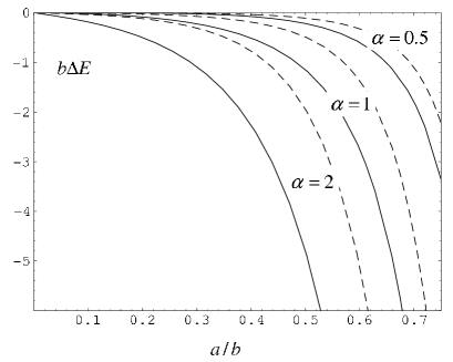
Figure 1: Interaction part of the vacuum energy as a function of $a/b$ for various values of the parameter $\alpha$. The full curves correspond to the massless fermionic field and the dashed curves are for the massive field with $Mb=1$.

5 Conclusion

In this paper we have studied the fermionic Casimir effect for the geometry of two spherical shells in a idealized point-like global monopole spacetime. The VEVs of the energy-momentum tensor and the fermionic condensate are investigated in the region between two spheres assuming that on the sphere surfaces the MIT bag boundary condition is satisfied. The unrenormalized expectation values are expressed as series over the zeros of a combination of the cylindrical functions given by formula (26) with the tilted notation from (25). To deal with this type of series, in Appendix A we derive summation formula by making use of the generalized Abel-Plana formula. The application of this formula to the corresponding mode-sums allowed us to extract from the VEVs the parts due to single spheres when the second sphere is absent and to present the additional part in terms of exponentially convergent integrals. In particular, the latter are convenient for numerical calculations. We have shown that the different parities for the fermionic eigenfunctions give the same contribution into the VEVs. For the points away from the boundaries, the boundary induced terms are unamiguously defined and the ambiguities in the renormalization procedure in the form of an arbitrary mass scale are contained in the boundary-free parts only. In particular, for a massless fermionic field the boundary induced energy-momentum tensor does not contain conformal anomalies and is traceless. We have discussed the behavior of the VEVs for the energy-momentum tensor and fermionic condensate in various limiting cases. In particular, for strong gravitational fields corresponding to small values of the parameter $\alpha$, these VEVs are exponentially suppressed. For large values $\alpha$ corresponding to the negative solid angle deficit, $\alpha\gg 1$, the VEVs tend to the finite limiting value. By using the radial vacuum stress, in section 3 we consider the vacuum forces acting on the spheres. These forces are presented in the form of the sum of self-action and interaction terms. Due to the surface divergences in the VEVs of the energy-momentum tensor, the self-action part of the vacuum force is divergent and needs further renormalization. This can be done by making use of zeta function renormalization technique. The interaction parts in the vacuum forces are finite for all non-zero distances between the spheres and are given by formula (61). An alternative representation for these forces is given by Eq. (63). The Casimir energy in the region between two spheres is considered in section 4. By using the zeta function technique we have presented it as the sum of the single sphere and interaction energies. The latter is given by formula (76) and is negative. We have explicitly checked that the interaction parts in the vacuum forces and in the vacuum energy are related by standard formula (77). In addition, we have shown that the interaction part of the vacuum energy evaluated from the sum of the zero-point energies of elementary oscillators coincides with the corresponding energy obtained by the integration of the local density. Note that for a scalar field, in general, this is not the case and in the discussion of the energy balance it is necessary to take into account the surface part of the energy located on the boundaries. We have investigated the interaction part of the vacuum energy in various limiting cases. First, we have checked that in the limit $a,b\to\infty$, with fixed $b-a$, the result for the geometry of parallel plates with bag boundary conditions in the Minkowski bulk is obtained. In the limit $a\to 0$ and for fixed values for the other parameters the interference part of the vacuum energy vanishes as $a^{2/\alpha}$. For large values $b$ this energy behaves like $b^{-2/\alpha-1}$ for a massless field and is exponentially suppressed for a massive field under the condition $Mb\gg 1$. For small values of the parameter $\alpha$ corresponding to strong gravitational fields the vacuum energy is suppressed by the factor $(a/b)^{2/\alpha}$. For large values $\alpha$ corresponding to a negative solid angle deficit, the interaction part of the vacuum energy per unit surface tends to the finite value given by formula (89).

Appendix A Appendix: Summation formulae over zeros of $C_{\nu}(\eta,z)$

As we have seen in section 2, for the massive spinor field in the region between two spheres the eigenmodes for the quantum number $k$ are expressed in terms of the zeros of the function

$$C_{\nu}(\eta,z)\equiv\tilde{J}_{\nu}^{(a)}(z)\tilde{Y}_{\nu}^{(b)}(\eta z)-\tilde{Y}_{\nu}^{(a)}(z)\tilde{J}_{\nu}^{(b)}(\eta z),$$ (90)

where the tilded quantities are defined as (25) and we will assume that $\eta>1$. To evaluate the VEV of the energy-momentum tensor we need to sum series over these zeros. Here we derive a summation formula for this type of series by making use of the generalized Abel-Plana formula derived in [14, 15]. In this formula as functions $g(z)$ and $f(z)$ we choose

$$g(z)=\frac{1}{2i}\left[\frac{\tilde{H}_{\nu}^{(1b)}(\eta z)}{\tilde{H}_{\nu}^{(1a)}(z)}+\frac{\tilde{H}_{\nu}^{(2b)}(\eta z)}{\tilde{H}_{\nu}^{(2a)}(z)}\right]\frac{h(z)}{C_{\nu}(\eta,z)},\quad f(z)=\frac{h(z)}{\tilde{H}_{\nu}^{(1a)}(z)\tilde{H}_{\nu}^{(2a)}(z)},$$ (91)

with the sum and difference

$$g(z)-(-1)^{n}f(z)=-i\frac{\tilde{H}_{\nu}^{(na)}(\eta z)}{\tilde{H}_{\nu}^{(na)}(z)}\frac{h(z)}{C_{\nu}(\eta,z)},\quad n=1,2.$$ (92)

The conditions for the generalized Abel-Plana formula written in terms of the function $h(z)$ are as follows

$$|h(z)|<\varepsilon_{1}(x)e^{c|y|},\quad|z|\to\infty,\quad z=x+iy,$$ (93)

where $c<2(\eta-1)$ and $\varepsilon_{1}(x)/x\to 0$ for $x\to+\infty$. Let $\gamma_{\nu,s}$ be positive zeros for the function $C_{\nu}(\eta,z)$. To find the residues of the function $g(z)$ at the poles $z=\gamma_{\nu,s}$ we need the derivative

$$\frac{\partial}{\partial z}C_{\nu}(\eta,z)=\frac{4}{\pi T_{\nu}^{ab}(\eta,z)}\frac{\tilde{J}_{\nu}^{(b)}(\eta z)}{\tilde{J}_{\nu}^{(a)}(z)}\,,\quad z=\gamma_{\nu,s},$$ (94)

where we have introduced the notation

$$T_{\nu}^{ab}(\eta,z)=z\left[\frac{\tilde{J}_{\nu}^{(a)2}(z)}{\tilde{J}_{\nu}^{(b)2}(\eta z)}D_{\nu}^{(b)}-D_{\nu}^{(a)}\right]^{-1},$$ (95)

with

$$D_{\nu}^{(w)}=w^{2}\left[k^{2}+(M-E)(M-n_{\sigma}\nu n^{(w)}/w)+\frac{n^{(w)}k^{2}}{2wE}\right],$$ (96)

and $ka=z$. By using this relation it can be seen that

$$\underset{z=\gamma_{\nu,s}}{\mathrm{Res}}g(z)=\frac{\pi}{4i}T_{\nu}^{ab}(\eta,\gamma_{\nu,s})h(\gamma_{\nu,s}).$$ (97)

Let $h(z)$ be an analytic function for $\mathrm{Re\,}z\geq 0$ except possible branch points on the imaginary axis. By using the generalized Abel-Plana formula, similar to the derivation of summation formula (4.13) in [15], it can be seen that if it satisfies condition (93),

$$h(ze^{\pi i})=-h(z)+o(z^{-1}),\quad z\to 0,$$ (98)

and the integral

$$\int_{0}^{L}\frac{h(x)dx}{\tilde{J}_{\nu}^{(a)2}(x)+\tilde{Y}_{\nu}^{(a)2}(x)}$$ (99)

exists, then

$$\lim_{L\to+\infty}\left\{\frac{\pi^{2}}{4}\sum_{s=1}^{m}h(\gamma_{\nu,s})T_{\nu}^{ab}(\eta,\gamma_{\nu,s})-\int_{0}^{L}\frac{h(x)dx}{\tilde{J}_{\nu}^{(a)2}(x)+\tilde{Y}_{\nu}^{(a)2}(x)}\right\}=$$ (100)

$$= -\frac{\pi}{2}\underset{z=0}{\mathrm{Res}}\left[\frac{h(z)\tilde{H}_{\nu}^{(1b)}(\eta z)}{C_{\nu}(\eta,z)\tilde{H}_{\nu}^{(1a)}(z)}\right]-\frac{\pi}{4}\sum_{\beta=\pm}\int_{0}^{\infty}dx\,\Omega_{a\nu}^{(\beta)}(x,\eta x)h(xe^{\beta\pi i/2}),$$

where $\gamma_{\nu,m}<L<\gamma_{\nu,m+1}$. Here the function $\Omega_{a\nu}^{(\beta)}(x,\eta x)$ is defined as

$$\Omega_{a\nu}^{(\beta)}(x,\eta x)=\frac{K_{\nu}^{(b\beta)}(\eta x)/K_{\nu}^{(a\beta)}(x)}{K_{\nu}^{(a\beta)}(x)I_{\nu}^{(b\beta)}(\eta x)-I_{\nu}^{(a\beta)}(x)K_{\nu}^{(b\beta)}(\eta x)},$$ (101)

and for a given function $F(z)$ we use the notation

$$F^{(w\pm)}(z)=zF^{\prime}(z)+\left[n^{(w)}\left(\mu_{w}-\sqrt{z^{2}e^{\pm\pi i}+\mu_{w}^{2}}\right)-n_{\sigma}\nu\right]F(z)\ .$$ (102)

In section 2, formula (100) is used to derive the VEV of the energy momentum-tensor for the region between two spherical shells in the global monopole spacetime. As it can be seen from expressions (31)–(33), the corresponding functions $h(z)$ satisfy the relation

$$h(xe^{\pi i/2})=-h(xe^{-\pi i/2})\ ,\quad\mathrm{for}\quad 0\leqslant x\leqslant\mu_{a}\ .$$ (103)

By taking into account that for these values $x$ one has $F^{(w+)}(wx/a)=F^{(w-)}(wx/a)$, we conclude that in this case the part of the integral on the right of Eq. (100) over the interval $(0,\mu_{a})$ vanishes.

References

• [1] T. W. Kibble, J. Phys. A 9, 1387 (1976).
• [2] A. Vilenkin, Phys. Rep. 121, 263 (1985).
• [3] D.D. Sokolov and A.A. Starobinsky, Dokl. Akad. Nauk USSR 234, 1043 (1977).
• [4] M. Barriola and A. Vilenkin, Phys. Rev. Lett. 63, 341 (1989).
• [5] G.E. Volovik, Pisma Zh. Eksp. Teor. Fiz. 67, 666 (1998) [JETP Lett. 67, 698 (1998)].
• [6] F.D. Mazzitelli and C.O. Lousto, Phys. Rev. D 43, 468 (1991).
• [7] E.R. Bezerra de Mello, V.B. Bezerra, and N.R. Khusnutdinov, Phys. Rev. D 60, 063506 (1999).
• [8] M. Bordag, K. Kirsten, and S. Dowker, Commun. Math. Phys. 128, 371 (1996).
• [9] J.S. Dowker and K. Kirsten, Commun. Anal. Geom. 7, 641 (1999).
• [10] F.C. Carvalho and E.R. Bezerra de Mello, Class. Quantum Grav. 18, 1637 (2001); Class. Quantum Grav. 18, 5455 (2001).
• [11] E.R. Bezerra de Mello, J. Math. Phys. 43, 1018 (2002).
• [12] E.R. Bezerra de Mello, V.B. Bezerra, and N.R. Khusnutdinov, J. Math. Phys. 42, 562 (2001).
• [13] A.A. Saharian and M.R. Setare, Class. Quantum Grav. 20, 3765 (2003).
• [14] A.A. Saharian, Izv. Akad. Nauk. Arm. SSR. Mat. 22, 166 (1987) [Sov. J. Contemp. Math. Anal. 22, 70 (1987)].
• [15] A.A. Saharian, ”The Generalized Abel-Plana Formula. Applications to Bessel functions and Casimir effect,” Report No. IC/2000; hep-th/0002239.
• [16] A.A. Saharian and E.R. Bezerra de Mello, J. Phys. A 37, 3543 (2004).
• [17] A.A. Saharian and M.R. Setare, Int. J. Mod. Phys. A 19, 4301 (2004).
• [18] C.M. Bender and P. Hays, Phys. Rev. D 14, 2622 (1976).
• [19] K.A. Milton, Phys. Rev. D 22, 1444 (1980).
• [20] K.A. Milton, Phys. Lett. B 104, 49 (1981).
• [21] K.A. Milton, Ann. Phys. (N.Y.) 150, 432 (1983).
• [22] J. Baacke and Y. Igarashi, Phys. Rev. D 27, 460 (1983).
• [23] S.K. Blau, M. Wisser, and A. Wipf, Nucl. Phys. B 310, 163 (1988).
• [24] E. Elizalde, M. Bordag, and K. Kirsten, J. Phys. A 31, 1743 (1998).
• [25] G. Cognola, E. Elizalde, and K. Kirsten, J. Phys. A 34, 7311 (2001).
• [26] A.A. Grib, S.G. Mamayev, and V.M. Mostepanenko, Vacuum Quantum Effects in Strong Fields (Friedmann Laboratory Publishing, St. Petersburg, 1994).
• [27] V.M. Mostepanenko and N.N. Trunov, The Casimir Effect and Its Applications (Oxford University Press, Oxford, 1997).
• [28] G. Plunien, B. Muller and W. Greiner, Phys. Rep. 134, 87 (1986).
• [29] K.A. Milton, The Casimir Effect: Physical Manifestation of Zero–Point Energy (World Scientific, Singapore, 2002).
• [30] M. Bordag, U. Mohidden, and V.M. Mostepanenko, Phys. Rep. 353, 1 (2001).
• [31] N.D. Birrell and P.C.W. Davies, Quantum Fields in Curved Space (Cambridge University Press, Cambridge, England, 1982).
• [32] V.B. Berestetskii, E.M. Lifshits, and L. P. Pitaevskii, Quantum Electrodynamics (Pergamon Press, Oxford, 1982).
• [33] A.P. Prudnikov, Yu.A. Brychkov, and O.I. Marichev, Integrals and Series (Gordon and Breach, New York, 1986), Vol.2.
• [34] E. Elizalde, S.D. Odintsov, A. Romeo, A.A. Bytsenko, and S. Zerbini, Zeta Regularization Techniques with Applications (World Scientific, Singapore, 1994).
• [35] K. Kirsten, Spectral Functions in Mathematics and Physics (Chapman and Hall/CRC, Boca Raton, 2002).
• [36] G. Kennedy, R. Critchley, and J.S. Dowker, Ann. Phys. (N.Y.) 125, 346 (1980); A. Romeo and A.A. Saharian, J. Phys. A 35, 1297 (2002); A.A. Saharian, Phys. Rev. D 63, 125007 (2001); S.A. Fulling, J. Phys. A 36, 6857 (2003); A.A. Saharian and M.R. Setare, Class. Quantum Grav. 21, 5261 (2004); A.A. Saharian, Phys. Rev. D 70, 064026 (2004); I. Cavero-Peláez, K.A. Milton, and J. Wagner, hep-th/0508001; A.A. Saharian and A.S. Tarloyan, hep-th/0603144.
• [37] A.A. Saharian, Phys. Rev. D 69, 085005 (2004).
• [38] M. Abramowitz and I.A. Stegun, Handbook of Mathematical Functions (National Bureau of Standards, Washington DC, 1964).