Non perturbative renormalisation group and momentum dependence of $n$-point functions (II)

Abstract

In a companion paper (hep-th/0512317), we have presented an approximation scheme to solve the Non Perturbative Renormalization Group equations that allows the calculation of the $n$-point functions for arbitrary values of the external momenta. The method was applied in its leading order to the calculation of the self-energy of the O($N$) model in the critical regime. The purpose of the present paper is to extend this study to the next-to-leading order of the approximation scheme. This involves the calculation of the 4-point function at leading order, where new features arise, related to the occurrence of exceptional configurations of momenta in the flow equations. These require a special treatment, inviting us to improve the straightforward iteration scheme that we originally proposed. The final result for the self-energy at next-to-leading order exhibits a remarkable improvement as compared to the leading order calculation. This is demonstrated by the calculation of the shift $\Delta T_{c}$, caused by weak interactions, in the temperature of Bose-Einstein condensation. This quantity depends on the self-energy at all momentum scales and can be used as a benchmark of the approximation. The improved next-to-leading order calculation of the self-energy presented in this paper leads to excellent agreement with lattice data and is within 4% of the exact large $N$ result.

I Introduction

The development of non-perturbative methods is essential to be able to deal with a large variety of problems in which the absence of a small parameter prevents one to build solutions in terms of a systematic expansion. Among such methods, the non perturbative renormalization group (NPRG) Wetterich93 ; Ellwanger93 ; Tetradis94 ; Morris94 ; Morris94c stands out as a very promising tool, suggesting new approximation schemes which are not easily formulated in other, more conventional, approaches in field theory or many body physics. The NPRG has been applied successfully to a variety of physical problems, in condensed matter, particle or nuclear physics (for reviews, see e.g. Bagnuls:2000ae ; Berges02 ; Canet04 ). In most of these problems however, the focus is on long wavelength modes and the solution of the NPRG equations involves generally a derivative expansion which only allows for the determination of the $n$-point functions and their derivatives at small external momenta (vanishing momenta in the case of critical phenomena). In many situations, this is not enough: a full knowledge of the momentum dependence of the correlation functions is needed to calculate the quantities of physical interest.

For this reason, in ref. alpha1 , we have presented an approximation scheme to solve the NPRG equations that allows the calculation of the $n$-point functions for arbitrary values of the external momenta. The method was applied in its leading order to the calculation of the self-energy of the O($N$) model in the critical regime. The purpose of the present paper is to extend this study to the next-to-leading order of the approximation scheme. This involves the calculation of the 4-point function at leading order, where new features arise. In particular we need to deal with exceptional configurations of momenta that enter the flow equations. Because of these, the straightforward iteration scheme proposed in ref. alpha1 yields some unphysical features in the 4-point function. After having identified the origin of the problem, we shall show how it can be cured by a proper treatment of the flow equation in the channel where the exceptional momenta matter. The final result for the self-energy at next-to-leading order exhibits a significant improvement as compared to the leading order calculation. In particular the calculation of the the shift $\Delta T_{c}$ in the transition temperature of the weakly repulsive Bose gas club , a quantity which is very sensitive to all momentum scales and which is used as a benchmark of the approximation, is now in excellent agreement with the available lattice data, and within 4% of the exact large $N$ result. Note that preliminary results concerning the calculation of $\Delta T_{c}$ at next-to-leading order have been presented in ref. Blaizot:2004qa . These results were obtained without the improvements just alluded to.

This paper is a sequel of ref. alpha1 , and should be read in conjunction with it (hereafter ref. alpha1 will be referred to as paper I, and the prefix I in equation labels will refer to equations in paper I). As in paper I we shall focus the discussion on the O($N$) model, although most of the arguments have a wider range of applicability. Thus, we shall consider a scalar $\varphi^{4}$ theory in $d$ dimension with $O(N)$ symmetry:

$${\cal S}=\int{\rm d}^{d}x\,\left\{{1\over 2}\left[\nabla\varphi(x)\right]^{2}+{1\over 2}r\varphi^{2}(x)+{u\over 4!}\left[\varphi^{2}(x)\right]^{2}\right\},$$ (1)

The field $\varphi(x)$ has $N$ real components $\varphi_{i}(x)$, with $i=1,\cdots,N$.

The basic equation of the NPRG is the flow equation for the effective action $\Gamma_{\kappa}[\phi]$ which interpolates between the classical action ${\cal S}$ and the full effective action $\Gamma[\phi]$ ($\phi$ is the expectation value of the field) as the parameter $\kappa$ varies from the microscopic scale $\Lambda$ down to zero. The flow equation for the effective action $\Gamma_{\kappa}[\phi]$ reads Wetterich93 ; Ellwanger93 ; Tetradis94 ; Morris94 ; Morris94c :

$$\partial_{\kappa}\Gamma_{\kappa}[\phi]={1\over 2}\,{\rm tr}\int{d^{d}q\over(2\pi)^{d}}\,\partial_{\kappa}R_{\kappa}(q^{2})\left[\Gamma_{\kappa}^{(2)}+R_{\kappa}\right]^{-1}_{q,-q},$$ (2)

where the trace runs over the O($N$) indices, $\Gamma_{\kappa}^{(2)}$ is the second derivative of $\Gamma_{\kappa}$ with respect to $\phi$, and $R_{\kappa}(q)$ is the regulator chosen, as in paper I, of the form Litim

$$R_{\kappa}(q)\propto(\kappa^{2}-q^{2})\theta(\kappa^{2}-q^{2}).$$ (3)

The role of the regulator is to suppress the fluctuations with momenta $q\mathrel{\hbox to0.0pt{\raise 2.20013pt\hbox{$<$}\hss}{\lower 2.20013pt\hbox{$\sim$}}}\kappa$, while leaving unaffected those with $q\mathrel{\hbox to0.0pt{\raise 2.20013pt\hbox{$>$}\hss}{\lower 2.20013pt\hbox{$\sim$}}}\kappa$.

The flow equations for the various $n$-point functions are obtained by taking functional derivatives with respect to $\phi$ of the equation for $\Gamma_{\kappa}[\phi]$ (see eq. (I.8)). In particular, the self-energy $\Sigma(\kappa;p)$ is obtained by integrating the flow equation (I.9):

$$\partial_{\kappa}\Gamma^{(2)}_{12}(\kappa;p)\equiv\delta_{12}\partial_{\kappa}\Sigma(\kappa;p)=-{1\over 2}\int{d^{d}q\over(2\pi)^{d}}\,\partial_{\kappa}R_{\kappa}(q)\,G^{2}(\kappa;q)\,\Gamma^{(4)}_{12ll}(\kappa;p,-p,q,-q),$$ (4)

with the inverse propagator given by

$$G^{-1}(\kappa,q)=q^{2}+\Sigma(\kappa;q)+R_{\kappa}(q).$$ (5)

In eq. (4), and later in this paper, we often denote the O($N$) indices simply by numbers $1,2,$ etc., instead of $i_{1},i_{2},$ etc., in order to alleviate the notation.

The flow equations for the $n$-point functions constitute an infinite hierarchy of coupled equations (for example, eq. (4) for the 2-point function contains in its r.h.s. the 4-point function). In paper I we have proposed a strategy to solve this hierarchy by following an iterative procedure. This starts with an initial ansatz for the $n$-point functions to be used in the right hand side of the flow equations. Integrating the flow equation of a given $n$-point function gives then the leading order (LO) estimate for that $n$-point function. Inserting the leading order of the $n$-point functions thus obtained in the right hand side of the flow equations and integrating gives then the next-to-leading order (NLO) estimate of the $n$-point functions. And so on.

Recall that there is no small parameter controlling the convergence of the process, and the terminology LO, NLO, refers merely to the number of iterations involved in the calculation of the $n$-point function considered. Since the calculations become increasingly complicated as the number of iterations increases, the success of the procedure relies crucially on the quality of the initial ansatz. A major task then is to construct such a good initial ansatz.

The equations are solved starting at the bottom of the hierarchy, that is, with the equation for the 2-point function which involves, in its right hand side, the 2-point function (through the propagator), and the 4-point function. As initial ansatz for the propagator, we take the propagator of a modified version of the derivative expansion that we called the LPA’; it is given by (see paper I, sect. II):

$$G_{LPA^{\prime}}^{-1}(\kappa;q)=Z_{\kappa}q^{2}+m_{\kappa}^{2}+R_{\kappa}(q),$$ (6)

where the field renormalization factor $Z_{\kappa}$ and the running mass $m_{\kappa}$ are obtained by solving the LPA’ equations (see paper I, sect. IIB). The initial ansatz for the 4-point function is given explicitly in paper I, sect. III, and is obtained as the solution of an approximate equation (see eq. (I.68) and eq. (II.1) below). For more clarity, we shall distinguish in this paper the initial ansatz for $\Gamma^{(4)}$ by a tilde. For consistency, we shall use a similar notation for the initial ansatz for the propagator, i.e., we shall set $\tilde{G}\equiv G_{LPA^{\prime}}$. Summarizing, the leading order self-energy is given by:

$$\delta_{12}\partial_{\kappa}\Sigma_{LO}(\kappa;p)=-{1\over 2}\int{d^{d}q\over(2\pi)^{d}}\,\partial_{\kappa}R_{\kappa}(q)\,\tilde{G}^{2}(\kappa;q)\,\tilde{\Gamma}^{(4)}_{12ll}(\kappa;p,-p,q,-q).$$ (7)

Note that, as compared to eq. (4), eq. (7) is now a trivial flow equation since all quantities in the r.h.s. are known quantities: $\Sigma_{LO}(\kappa;p)$ is simply obtained by integrating the r.h.s. with respect to $\kappa$. The leading order self-energy has been studied in detail in paper I.

As stated earlier, the purpose of the present paper is to calculate $\Sigma_{NLO}(p)$, the self-energy at next-to-leading order. To do so, we need to use in the r.h.s of eq. (4) the leading order expressions for both the propagator and the 4-point function. The leading order propagator is obtained from eq. (5) with the self-energy $\Sigma_{LO}$. Getting the leading order expression for the 4-point function $\Gamma^{(4)}_{12ll}(\kappa;p,-p,q,-q)$ will be the main task of this paper; it is presented in sect. II. First, in sect. II.1, we follow the procedure outlined above, i.e., replace in the r.h.s. of the flow equation for the 4-point function, eq. (II) below, the initial ansatz for the propagator, the 4- and the 6-point functions. The initial ansatz for the 6-point function is obtained by following the same strategy as that used in paper I, sec. III, in order to construct the initial ansatz for the 4-point function. Although conceptually straightforward, this is technically more involved and the details are presented in app. A. Then, in sec. II.2, we present an improved procedure to calculate $\Gamma^{(4)}_{12ll}(\kappa;p,-p,q,-q)$ at LO, which copes properly with the difficulties related to the exceptional configuration of momenta. The properties of $\Sigma_{NLO}$ are presented in sect. III, together with the result of the calculation of $\Delta\langle\varphi^{2}\rangle$, which we use, as we have recalled earlier, as a benchmark of the approximation scheme. The last section summarizes the results, and points to further improvements of the approximation scheme that we have already started to implement PLB ; BMWn .

II The 4–point function at LO

The flow equation for the the 4-point function in vanishing field reads (see e.g. eq. (I.11)):

$$\partial_{\kappa}\Gamma^{(4)}_{12ll}(\kappa;p,-p,q,-q)=\int{d^{d}q^{\prime}\over(2\pi)^{d}}\partial_{\kappa}R_{\kappa}(q^{\prime})G^{2}(\kappa;q^{\prime})$$

$$\hskip 14.22636pt\times\left\{G(\kappa;q^{\prime})\Gamma^{(4)}_{12ij}(\kappa;p,-p,q^{\prime},-q^{\prime})\Gamma^{(4)}_{llij}(\kappa;q,-q,-q^{\prime},q^{\prime})\right.$$

$$\hskip 14.22636pt+G(\kappa;q^{\prime}+p+q)\Gamma^{(4)}_{1lij}(\kappa;p,q,q^{\prime},-q^{\prime}-p-q)\Gamma^{(4)}_{2lij}(\kappa;-p,-q,-q^{\prime},q^{\prime}+p+q)$$

$$\hskip 14.22636pt\left.+G(\kappa;q^{\prime}+p-q)\Gamma^{(4)}_{1lij}(\kappa;p,-q,q^{\prime},-q^{\prime}-p+q)\Gamma^{(4)}_{l2ij}(\kappa;q,-p,-q^{\prime},q^{\prime}-q+p)\right\}$$

$$\hskip 14.22636pt-{1\over 2}\int{d^{d}q\over(2\pi)^{d}}\partial_{\kappa}R_{\kappa}(q^{\prime})G^{2}(\kappa;q^{\prime})\Gamma^{(6)}_{12llmm}(\kappa;p,-p,q,-q,q^{\prime},-q^{\prime}).$$ (8)

We have specified here the O($N$) indices and the momenta of the particular 4-point function $\Gamma_{12ll}^{(4)}(\kappa;p,-p,q,-q)$ that is needed for the calculation of $\Sigma_{NLO}(p)$ (see e.g. eq. (4)). Following the terminology introduced in paper I, we refer to the second line of eq. (II) as to the $s$-channel contribution, while the third and fourth lines are respectively the $t$ and $u$-channel contributions. Note that the contribution of the $u$-channel differs from that of the $t$-channel solely by the change of sign of $q$. A graphical illustration of these various contributions is given in figs. 1-3.

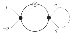
Figure 1: Diagrammatic illustration of the contribution of the $s$-channel to the flow of the 4-point function (the second line in eq. (II)). The dotted line indicates the loop integral involving this contribution of $\Gamma^{(4)}$ in the calculation of the self-energy in NLO, i.e., $\Sigma_{NLO}^{[s]}(p)$ (see sect. III).

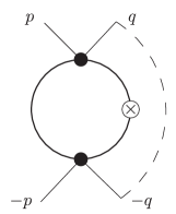
Figure 2: Diagrammatic illustration of the contribution of the $t$ and $u$ channels to the flow of the 4-point function (third and fourth lines in eq. (II)). The dashed line indicates the loop integral involving this contribution of $\Gamma^{(4)}$ in the calculation of the self-energy in NLO, i.e., $\Sigma_{NLO}^{[t+u]}(p)$ (see sect. III).

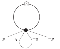
Figure 3: Diagrammatic illustration of the contribution of the 6-point function to the flow of the 4-point function (last line in eq. (II)). The dotted line indicates the loop integral involving this contribution of $\Gamma^{(4)}$ in the calculation of the self-energy in NLO, i.e., $\Sigma_{NLO}^{[6]}(p)$ (see sect. III).

As stated above, the leading order expression for $\Gamma^{(4)}$ is obtained by substituting in the r.h.s. of eq. (II) the initial ansatz for $G$, $\Gamma^{(4)}$ and $\Gamma^{(6)}$. In fact, we shall proceed with a further simplification which consists in setting $q^{\prime}=0$ in the vertices of the r.h.s. of eq. (II). For $\tilde{\Gamma}^{(4)}$, this is justified by the fact that the initial anstaz $\tilde{\Gamma}^{(4)}$ varies little when the momenta on which it depends are varied by an amount smaller than $\kappa$. This property has been explicitly assumed in the construction of $\tilde{\Gamma}^{(4)}$ in paper I. It has also been tested quantitatively in the calculation of the leading order self-energy (see fig. 15 in paper I and the discussion at the end of sect. IV of paper I). We assume that this property also holds for the initial ansatz $\tilde{\Gamma}^{(6)}_{12llmm}(\kappa;p,-p,q,-q,q^{\prime},-q^{\prime})$. In fact, for this latter function we shall also set $q=0$, which can be justified as follows. Note first that $\Gamma^{(4)}(p,-p,q,-q)$ will eventually be used in the calculation of $\Sigma_{NLO}(p)$, and in this calculation $q\mathrel{\hbox to0.0pt{\raise 2.20013pt\hbox{$<$}\hss}{\lower 2.20013pt\hbox{$\sim$}}}\kappa$. As we explained in paper I, sect. IIIA, setting $q=0$ is then well justified when $p\mathrel{\hbox to0.0pt{\raise 2.20013pt\hbox{$<$}\hss}{\lower 2.20013pt\hbox{$\sim$}}}\kappa$, because in that case all the momenta are smaller than $\kappa$, and $\Gamma^{(6)}$ is well approximated by the LPA’; it is also justified when $p\gg\kappa$ since then $q$ is negligible compared to $p$. It is only in the small integration region $q\sim\kappa$ that the approximation could be less accurate. Observe finally that the contribution of $\Gamma^{(6)}$ is negligible unless $p\ll\kappa_{c}$. Thus, in line with approximation ${\cal A}_{1}$ of paper I, we shall, in the r.h.s. of eq. (II), set $q^{\prime}=0$ in the 4-point functions $\tilde{\Gamma}^{(4)}$ and $q=q^{\prime}=0$ in $\tilde{\Gamma}^{(6)}$. We then arrive at the following simplified equation:

$$\kappa\partial_{\kappa}\Gamma^{(4)}_{12ll}(\kappa;p,-p,q,-q)=I_{d}^{(3)}(\kappa)\tilde{\Gamma}^{(4)}_{12ij}(\kappa;p,-p,0,0)\tilde{\Gamma}^{(4)}_{llij}(\kappa;q,-q,0,0)$$

$$\hskip 14.22636pt+J_{d}^{(3)}(\kappa;p+q)\tilde{\Gamma}^{(4)}_{1lij}(\kappa;p,q,0,-p-q)\tilde{\Gamma}^{(4)}_{2lij}(\kappa;-p,-q,0,p+q)$$

$$\hskip 14.22636pt+J_{d}^{(3)}(\kappa;p-q)\tilde{\Gamma}^{(4)}_{1lij}(\kappa;p,-q,0,-p+q)\tilde{\Gamma}^{(4)}_{2lij}(\kappa;-p,q,0,p-q)$$

$$\hskip 14.22636pt-{1\over 2}I_{\rm d}^{(2)}(\kappa)\tilde{\Gamma}^{(6)}_{12llmm}(\kappa;p,-p,0,0,0,0),$$ (9)

where the functions $I_{d}^{(n)}(\kappa)$ and $J_{d}^{(n)}(\kappa;p)$ are defined in eqs. (I.42) and (I.55), respectively. The construction of the initial ansatz $\tilde{\Gamma}^{(6)}_{12llmm}(\kappa;p,-p,0,0,0,0)$ requires the solution of an approximate flow equation which is obtained by following the same three approximations that are used in paper I, sect. III, to get $\tilde{\Gamma}^{(4)}$. This is presented in app. A. The explicit traces of products of the functions $\tilde{\Gamma}^{(4)}$ appearing in eq. (II) are given in app. B.

Eq. (II) will be used to calculate $\Gamma^{(4)}$ at LO. Note that, as was the case for eq. (7) giving $\Sigma_{LO}$, eq. (II) is now a trivial flow equation: all quantities in its r.h.s. are known quantities. We shall refer to this calculation of $\Gamma^{(4)}$ at LO, which follows strictly the scheme proposed in paper I, as to the “direct procedure”. The results obtained in this way are discussed in the next subsection. We shall see there that this procedure yields unphysical features in some specific situations, whose origin will be discussed. An improvement on the direct procedure will then be proposed in the following subsection.

Before proceeding further, let us mention that we have used the LO estimate of $\Gamma_{12ll}^{(4)}(\kappa,p,-p,q,-q)$ obtained in the direct procedure to perform a consistency check of approximation ${\cal A}_{1}$ used in order to obtain eq. (II). We have verified that $\Gamma_{12ll}^{(4)}(\kappa,p,-p,q,-q)$ varies little as $q$ varies in the range $q<\kappa$, which is the range relevant for the calculation of $\Sigma_{NLO}(p)$. Only in a small region where $\kappa$ is of order $p\ll\kappa_{c}$, can the function change by as much as 10% when $q$ goes from 0 to $\kappa$. In all the other regions the variation is less than 1%. In the calculation of $\Delta\langle\varphi^{2}\rangle$ that will be reported in the next section, one needs $\Sigma_{NLO}(p)$ for values of $p$ around $\kappa_{c}$: there, the approximation ${\cal A}_{1}$ is indeed excellent. However, at very small momenta, the error due to this approximation on the magnitude of $\Sigma_{NLO}(p)$ can be large. But in this region the approximation ${\cal A}_{1}$ is not the dominant source of error anyway: in particular, any error on the exponent $\eta$ will translate into a large relative error on the magnitude of $\Sigma_{NLO}(p)$.

II.1 Direct procedure

As we have just discussed, since all quantities in the r.h.s. of eq. (II) are known, $\Gamma_{12ll}^{(4)}(\kappa;p,-p,q,-q)$ at LO is obtained by simply integrating the r.h.s. of eq. (II) between $\Lambda$ and $\kappa$, and adding the bare value of $\Gamma^{(4)}$ (i.e., the value of $\Gamma^{(4)}$ at the microscopic scale $\Lambda$):

$$\Gamma_{12ll}^{(4)}(\kappa=\Lambda;p,-p,q,-q)=(N+2)\;g_{\Lambda}\;\delta_{12}$$ (10)

with $g_{\Lambda}=u/3$, $u$ being the parameter of the classical action (1) (see paper I, sect. IIB).

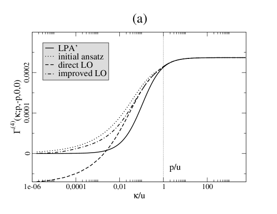
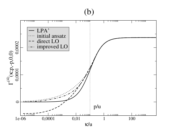
Figure 4: The 4-point function $\Gamma^{(4)}(\kappa;p,-p,0,0)$ (in units of $\Lambda$) as a function of $\kappa/u$: the four curves represent respectively the LPA’ (full line), the initial ansatz (dotted line), the direct LO (dashed line) and the improved LO (dot-dashed line). The calculation is done for (a): $p=\;u$, and (b): $p=\;u/10$.

The LO value of $\Gamma^{(4)}_{12ll}(\kappa,p,-p,0,0)$ thus obtained is compared with both the initial ansatz and the LPA’ result, $(N+2)g_{\kappa}$, in fig. 4 below. When $\kappa\mathrel{\hbox to0.0pt{\raise 2.20013pt\hbox{$>$}\hss}{\lower 2.20013pt\hbox{$\sim$}}}p$ one expects the LPA’ to be a good approximation, and indeed the three curves almost coincide (the initial ansatz is by construction identical to the LPA’ for large $\kappa$). When $\kappa$ goes to values smaller than $p$, the flow of the 4-point function is expected to be slower than that of the LPA’ since, generally, momenta in the propagators tend to suppress the flow. Fig. 4 shows that it is indeed the case (in the initial ansatz this feature is implemented in a sharp manner with the help of $\Theta$-functions depending on a parameter $\alpha$ (see paper I, sect. III, and eq. (II.1) below)). As shown by fig. 4, as $\kappa/p$ decreases further, the LO curve remains close to that corresponding to the initial ansatz but when $\kappa/p$ becomes too small, eventually the two curves deviate: while the initial ansatz goes to zero as $\kappa\to 0$, the LO curve goes to a negative value. As we shall explain shortly this is an unphysical feature of the LO in the direct procedure.

At this point, it is instructive to recall the form of the approximate flow equation whose solution is the initial ansatz $\tilde{\Gamma}^{(4)}$. This equation is established in paper I, sect. III, and reads (see eq. (I.68)):

$$\kappa\partial_{\kappa}\tilde{\Gamma}^{(4)}_{12ll}(\kappa;p,-p_{,}q,-q)=I_{d}^{(3)}(\kappa)\,(1-F_{\kappa})$$

$$\hskip 14.22636pt\times\left\{\tilde{\Gamma}^{(4)}_{12ij}(p,-p,0,0)\tilde{\Gamma}^{(4)}_{llij}(q,-q,0,0)\right.$$

$$\hskip 14.22636pt+\;\;\;\Theta\left({\kappa^{2}}-\alpha^{2}{(p+q)^{2}}\right)\tilde{\Gamma}^{(4)}_{1lij}(p,q,0,-p-q)\tilde{\Gamma}^{(4)}_{2lij}(-p,-q,0,p+q)$$

$$\hskip 14.22636pt\left.+\;\;\;\Theta\left({\kappa^{2}}-\alpha^{2}{(p-q)^{2}}\right)\tilde{\Gamma}^{(4)}_{1lij}(p,-q,0,-p+q)\tilde{\Gamma}^{(4)}_{2lij}(-p,q,0,p-q)\right\}.$$

The function $F_{\kappa}$ is defined in eq. (I.44). It measures (approximately) the magnitude of the contribution of the 6-point function relative to that of the terms containing the 4-point functions. Note the similarity between the r.h.s. of eq. (II) giving the LO expression of $\Gamma^{(4)}$ and the r.h.s. of eq. (II.1) for the initial ansatz $\tilde{\Gamma}^{(4)}$: the main differences are the replacement of the $\Theta$-functions of eq. (II.1) by the proper loop integrals in eq. (II), and a more accurate treatment of the contribution of the 6-point function in eq. (II). This observation leads us to expect that $\Gamma^{(4)}$ at LO should not differ much from $\tilde{\Gamma}^{(4)}$, a necessary condition for the validity of the iteration procedure. As shown by fig. 4, this expectation is fulfilled, except for small values of $\kappa$: while the LO $\Gamma^{(4)}$ goes to a negative value when $\kappa\to 0$, the initial ansatz $\tilde{\Gamma}^{(4)}(\kappa;p,-p,0,0)$ vanishes (one reads from eq. (I.99) that in the limit $\kappa\to 0$, $\tilde{\Gamma}^{(4)}(\kappa;p,-p,0,0)$ goes to zero like $g_{\kappa}^{(N+2)/(N+8)}$). There is in fact a major difference between eq. (II.1) for the initial ansatz and eq. (II) giving $\Gamma^{(4)}$ at leading order: while in eq. (II.1) the unknown function $\tilde{\Gamma}^{(4)}(\kappa;p,-p,0,0)$ sits in the r.h.s, this is not so in eq. (II), as we have already emphasized. Thus the structures of eqs. (II.1) and (II) are different, and only eq. (II.1) captures the essential feature that guarantees the vanishing of $\tilde{\Gamma}^{(4)}(\kappa;p,-p,0,0)$ as $\kappa\to 0$, which, as we shall show now, is a property of the exact solution of the flow equation.

To do so, we shall consider eq. (II) for $\Gamma^{(4)}(\kappa;p,-p,0,0)$ and study the behaviour of its solution in the limit when $\kappa\to 0$. Observe first that the $s$-channel controls the flow when $\kappa\mathrel{\hbox to0.0pt{\raise 2.20013pt\hbox{$<$}\hss}{\lower 2.20013pt\hbox{$\sim$}}}p$: indeed, in this channel, the exceptional configuration of momenta $(p,-p)$ makes the loop integral in the r.h.s. of the flow equation independent of $p$. This is manifest in eq. (II): the loop integral reduces to the momentum independent function $I_{d}^{(3)}(\kappa)$, while in the other channels the $p$-dependent functions $J_{d}^{(3)}(p\pm q)$ enter (this is also obvious in eq. (II.1) where the functions $J_{d}^{(3)}(p\pm q)$ are approximated using $\Theta$-functions). It follows that in the $s$-channel, the external momentum $p$ does not contribute to stabilize the flow whenever $\kappa\mathrel{\hbox to0.0pt{\raise 2.20013pt\hbox{$<$}\hss}{\lower 2.20013pt\hbox{$\sim$}}}p$, as it does in the other channels: the flow continues all the way down to $\kappa=0$. When treated correctly, this is what induces the vanishing of $\Gamma^{(4)}(\kappa;p,-p,0,0)$. To show this latter point, we focus on the contribution of the $s$-channel and, in the r.h.s. of eq. (II) we keep $\Gamma^{(4)}(\kappa;p,-p,0,0)$ as an unknown function (instead of replacing it by the initial ansatz $\tilde{\Gamma}^{(4)}(\kappa;p,-p,0,0))$. We also temporarily neglect the contribution of the other two channels, and also the contribution of the 6-point function. Then, eq. (II) takes the following simple form (here we focus on the structure of the equation, dropping the O($N$) indices for simplicity, as well as explicit reference to the external momenta; a more precise equation is written in the next subsection):

$$\kappa\partial_{\kappa}\Gamma(\kappa)=g_{\kappa}I_{3}^{(3)}(\kappa)\,\Gamma(\kappa),$$ (12)

where we have replaced $\tilde{\Gamma}^{(4)}(\kappa;0,0,0,0)$ by the LPA vertex $g_{\kappa}$ (see eq. (19) below). In the limit $\kappa\to 0$ (see paper I), $g_{\kappa}\sim Z_{\kappa}^{2}\;\kappa^{4-d}$ and $I_{d}^{(3)}(\kappa)\sim\kappa^{d-4}/Z_{\kappa}^{2}$, so that $g_{\kappa}I_{d}^{(3)}(\kappa)\to\xi$, where $\xi$ is a positive constant. It then follows form eq. (12) that $\Gamma(\kappa)\sim\kappa^{\xi}$ as $\kappa\to 0$, and hence vanishes as $\kappa$ vanishes. Turning now to the contributions of the $t$ and $u$-channels, we note that these are more regular than the $s$-channel contribution (this can be seen for instance from the fact that the ratio $J_{d}^{(3)}(\kappa;p)/I_{d}^{(3)}(\kappa)\to 0$ as $\kappa/p\to 0$; see paper I, fig. 9). Similarly, the contribution of the 6-point function is proportional to $I_{d}^{(2)}$ and $I_{d}^{(2)}/I_{d}^{(3)}\sim\kappa^{2-2\eta}$ as $\kappa\to 0$. Using these properties, one can write the equation for the 4-point function at small $\kappa$ in the schematic form

$$\kappa\partial_{\kappa}\Gamma(\kappa)=\xi\,\Gamma(\kappa)+\Phi(\kappa),$$ (13)

where $\Phi(\kappa)$ may be considered at this point as a known function of $\kappa$ ($\Phi(\kappa)$ is constructed from the initial ansatz for the 4-point and 6-point functions). The equation above can be easily solved, with the result

$$\Gamma(\kappa)=\left[\Gamma(\kappa_{0})+\int^{\kappa}_{\kappa_{0}}{d\kappa^{\prime}\over\kappa^{\prime}}\Phi(\kappa^{\prime})\left({\kappa_{0}\over\kappa^{\prime}}\right)^{\xi}\right]\left({\kappa\over\kappa_{0}}\right)^{\xi}.$$ (14)

Since, as we have just argued, $\Phi(\kappa)$ vanishes as $\kappa\to 0$, the integral does not diverge faster than $\kappa^{-\xi}$, and the small $\kappa$ behavior is governed by the factor outside the brackets, that is by the solution of eq. (12), which guarantees that $\Gamma(0)=0$. This argument shows also that provided one solves consistently eq. (13) small errors in the estimate of the function $\Phi$ are damped by the factor $(\kappa/\kappa_{0})^{\xi}$. In particular, the solution for the initial ansatz is identical to that written above, eq. (14), with $\Phi$ replaced by another function $\tilde{\Phi}$ not too different from $\Phi$ (we may ignore here the factor $F(\kappa)$ in eq. (II.1), which complicates the analysis, but in an inessential way. Accordingly we can also ignore the contribution of the 6-point function in eq. (II). Then the only difference between eqs. (II.1) and (II) comes from the approximation of the functions $J^{(3)}_{3}$ of eq.(II) with the functions $\Theta$ in eq. (II.1)). One then expects the two solutions corresponding to $\Phi$ and $\tilde{\Phi}$ to be close to each other.

Let us however imagine that we apply the direct procedure to our schematic equations, by caculating $\Gamma_{LO}$ from the analog of eq. (II), namely

$$\kappa\partial_{\kappa}\Gamma_{LO}(\kappa)=\xi\tilde{\Gamma}(\kappa)+\Phi(\kappa)=\kappa\partial_{\kappa}\tilde{\Gamma}(\kappa)+\Phi(\kappa)-\tilde{\Phi}(\kappa),$$ (15)

where we have used the fact that $\kappa\partial_{\kappa}\tilde{\Gamma}(\kappa)=\xi\tilde{\Gamma}(\kappa)+\tilde{\Phi}(\kappa)$. We would then obtain

$$\Gamma_{LO}(\kappa)-\tilde{\Gamma}(\kappa)=\int_{\kappa_{0}}^{\kappa}{d\kappa^{\prime}\over\kappa^{\prime}}\left(\Phi(\kappa^{\prime})-\tilde{\Phi}(\kappa^{\prime})\right)$$ (16)

where the integral is convergent and yields a finite value for $\Gamma_{LO}(\kappa=0)$. Thus, although the two solutions $\Gamma(\kappa)$ and $\tilde{\Gamma}(\kappa)$ would differ little if $\Phi$ and $\tilde{\Phi}$ differ little, the direct procedure which consists in simply integrating the r.h.s. of the flow equation fails to reproduce the low $\kappa$ behavior. This small $\kappa$ behavior can only be obtained if the feedback of the flow is properly taken in the solution of the flow equation. But, as revealed in the previous analysis, this needs to be done only in the channel where the flow is not controlled by the external momenta, i.e., the $s$-channel. We shall implement this improved strategy for the LO in the next subsection.

II.2 Improved approximation for $\Gamma^{(4)}_{12ll}(\kappa;p,-p,0,0)$

As we have seen, the main problem with the direct procedure that we have followed in the previous subsection comes from the $s$-channel where the exceptional configuration of momenta does not contribute to stabilize the flow when $\kappa\to 0$. In this subsection and the following one, we shall present a more accurate treatment of this particular situation, making more precise the treatment presented in the previous subsection.

To this aim, we consider first the case $q=0$ and replace eq. (II) by:

$$\kappa\partial_{\kappa}\Gamma^{(4)}_{12ll}(\kappa;p,-p,0,0)=I_{d}^{(3)}(\kappa)\Gamma^{(4)}_{12ij}(\kappa;p,-p,0,0)\tilde{\Gamma}^{(4)}_{llij}(\kappa;0,0,0,0)+\Phi_{12}(\kappa;p),$$ (17)

where we have isolated the contribution of the $s$-channel, and grouped the other contributions into the function $\Phi_{12}(\kappa;p)$:

$$\Phi_{12}(\kappa,p) \equiv J_{d}^{(3)}(\kappa;p)\tilde{\Gamma}^{(4)}_{1lij}(\kappa;p,0,0,-p)\tilde{\Gamma}^{(4)}_{2lij}(\kappa;-p,0,0,p)$$ (18)

$$+ J_{d}^{(3)}(\kappa;p)\tilde{\Gamma}^{(4)}_{1lij}(\kappa;p,0,0,-p)\tilde{\Gamma}^{(4)}_{2lij}(\kappa;-p,0,0,p)$$

$$- {1\over 2}I_{d}^{(2)}(\kappa)\tilde{\Gamma}^{(6)}_{12llmm}(\kappa;p,-p,0,0,0,0).$$

$\Phi_{12}(\kappa,p)$ is a known function which involves the initial ansatz $\tilde{\Gamma}^{(4)}$ and $\tilde{\Gamma}^{(6)}$. In contrast, $\Gamma^{(4)}_{12ll}(\kappa;p,-p,0,0)$ is taken to be the same function in the r.h.s and the l.h.s. of eq. (17). That is, eq. (17) properly takes into account the feedback of the flow in the $s$-channel on the solution of the flow equation. Note that for $p=0$ the solution of eq. (17) (or eq. (II)) is the LPA solution. We can therefore replace in the r.h.s. of eq. (17) $\tilde{\Gamma}^{(4)}_{ijkl}(\kappa;0,0,0,0)$ by the LPA value

$$\tilde{\Gamma}^{(4)}_{ijkl}(\kappa;0,0,0,0)=g(\kappa)(\delta_{ij}\delta_{kl}+\delta_{ik}\delta_{jl}+\delta_{il}\delta_{jk}).$$ (19)

Then eq. (17) becomes

$$\kappa\partial_{\kappa}\Gamma^{(4)}(\kappa;p)=(N+2)I_{d}^{(3)}(\kappa)g(\kappa)\Gamma^{(4)}(\kappa;p)+\Phi(\kappa;p),$$ (20)

where we used the definitions

$$\Gamma^{(4)}_{12ll}(\kappa;p,-p,0,0)\equiv\delta_{12}\Gamma^{(4)}(\kappa;p),\hskip 28.45274pt\Phi_{12}(\kappa;p)=\delta_{12}\Phi(\kappa;p),$$ (21)

and we omitted a factor $\delta_{12}$ in both sides of eq. (20).

Eq. (20) is a linear differential equation in $\kappa$, with a non-homogenous term $\Phi$, depending on a parameter $p$. The general solution of the homogenous equation is:

$$\Gamma^{(4)}(\kappa;p)=\Gamma^{(4)}(\kappa_{0};p)\;e^{\int_{\kappa_{0}}^{\kappa}{d\kappa^{\prime}\over\kappa^{\prime}}\gamma(\kappa^{\prime})},$$ (22)

where

$$\gamma(\kappa)\equiv(N+2)I_{d}^{(3)}(\kappa)g(\kappa).$$

Note that, as $\kappa\to 0$, $\gamma(\kappa)\sim\xi$ with $\xi>0$. The value of $\kappa_{0}$ is to be chosen large enough for the LPA solution to remain a good approximation at this value of $\kappa$ (for example, $\kappa_{0}=10\;p$).

A particular solution of the total equation can be found in the form:

$$\Gamma^{(4)}(\kappa;p)=\hat{\Gamma}^{(4)}(\kappa;p)\;e^{\int_{\kappa_{0}}^{\kappa}{d\kappa^{\prime}\over\kappa^{\prime}}\gamma(\kappa^{\prime})}.$$ (23)

One gets

$$\hat{\Gamma}^{(4)}(\kappa;p)=\int_{\kappa_{0}}^{\kappa}{d\kappa^{\prime\prime}\over\kappa^{\prime\prime}}\Phi(\kappa^{\prime\prime},p)\;e^{-\int_{\kappa_{0}}^{\kappa^{\prime\prime}}{d\kappa^{\prime}\over\kappa^{\prime}}\gamma(\kappa^{\prime})}+\Gamma^{(4)}(\kappa_{0};p),$$ (24)

so that the general solution of equation (20) can be written as

$$\Gamma^{(4)}(\kappa;p)=\left[\int_{\kappa_{0}}^{\kappa}{d\kappa^{\prime}\over\kappa^{\prime}}\Phi(\kappa^{\prime};p)\;e^{-\int_{\kappa_{0}}^{\kappa^{\prime}}{d\kappa^{\prime\prime}\over\kappa^{\prime\prime}}\gamma(\kappa^{\prime\prime})}+\Gamma^{(4)}(\kappa_{0};p)\right]\;e^{\int_{\kappa_{0}}^{\kappa}{d\kappa^{\prime}\over\kappa^{\prime}}\gamma(\kappa^{\prime})}.$$ (25)

This expression has the expected behavior: the last exponential in the r.h.s. guarantees that $\Gamma^{(4)}(\kappa,p)\to 0$ as a power law when $\kappa\to 0$.

The behavior of the solution is shown in fig. 4 above and compared with the other expressions that we had for $\Gamma^{(4)}$, for the particular values $p=u$ and $p=u/10$. One can appreciate the effect of the improved procedure: the corresponding curve follows the direct LO one down to $\kappa\sim p/10$, then it correctly goes to zero when $\kappa\to 0$ while the direct LO one does not. This analysis confirms the importance of keeping the feedback of the flow in the $s$-channel, that is, of solving the flow equation in this channel, in order to get the correct behavior at $\kappa\to 0$.

As suggested by fig. 4, the range of values of $\kappa$ where $\Gamma^{(4)}(\kappa;p,-p,0,0)$ obtained in the direct procedure exhibits its pathological behavior decreases as $p$ decreases. In fact, as $p\to 0$, $\Gamma^{(4)}(\kappa;p,-p,0,0)\to 0$ as $\kappa\to 0$ (since the 4-point function is then given by the LPA’). One can argue at this point that the unphysical behavior of $\Gamma^{(4)}(\kappa)$ at small $\kappa$ has a moderate influence on the calculation of the NLO result for the self-energy. Indeed, as we shall see, it is mostly the region $\kappa\sim p$ that contributes significantly to the flow of $\Sigma_{NLO}(p)$; in this region, the estimates of the 4-point function obtained in the direct and improved LO are almost identical (the difference with the initial ansatz is also small). This is why we have used the direct procedure in the first estimate of $\Sigma_{NLO}$ presented in Blaizot:2004qa . However, as we shall see in the next section, the improved procedure turns out to be much more accurate.

II.3 Improved calculation of $\Gamma^{(4)}(\kappa;p,-p,q,-q)$

The procedure described in the previous subsection only applies to the 4-point function at $q=0$. It is only for this value of $q$ that we can write eq. (II) as a closed equation: if $q\neq 0$, the 4-point function in the l.h.s. and those in the r.h.s. are evaluated in different momentum configurations. However, we note that, in the calculation of $\Sigma_{NLO}(\kappa;p)$, we need $\Gamma^{(4)}(\kappa;p,-p,q,-q)$ only for $q<\kappa$, i.e., in a range of values of $q$ that vanishes as $\kappa\to 0$. In that range, we expect $\Gamma^{(4)}(\kappa;p,-p,q,-q)$ to differ very little from $\Gamma^{(4)}(\kappa;p,-p,0,0)$. Proceeding as in the previous subsection, we single out the $s$-channel and rewrite eq. (II) as

$$\kappa\partial_{\kappa}\Gamma^{(4)}_{12ll}(\kappa;p,-p,q,-q)=I_{d}^{(3)}(\kappa)\Gamma^{(4)}_{12ij}(\kappa;p,-p,0,0)\Gamma^{(4)}_{llij}(\kappa;q,-q,0,0)+\Phi_{12}(\kappa,p,q)$$ (26)

where, now

$$\Phi_{12}(\kappa,p,q) = J_{d}^{(3)}(\kappa;p+q)\tilde{\Gamma}^{(4)}_{1lij}(\kappa;p,q,0,-p-q)\tilde{\Gamma}^{(4)}_{2lij}(\kappa;-p,-q,0,p+q)$$

$$+ J_{d}^{(3)}(\kappa;p-q)\tilde{\Gamma}^{(4)}_{1lij}(\kappa;p,-q,0,-p+q)\tilde{\Gamma}^{(4)}_{2lij}(\kappa;-p,q,0,p-q)$$

$$- {1\over 2}I_{d}^{(2)}(\kappa)\tilde{\Gamma}^{(6)}_{12llmm}(\kappa;p,-p,q,-q,0,0)$$

$$\equiv \delta_{12}\Phi(\kappa;p,q).$$

In eq. (26), we use the fact that $q<\kappa$ to replace $\Gamma^{(4)}_{llij}(\kappa;q,-q,0,0)$ by the initial ansatz (we have seen earlier that this is a good approximation):

$$\Gamma^{(4)}_{llij}(\kappa;q,-q,0,0)\rightarrow(N+2)\delta_{ij}g(\kappa).$$ (28)

As a result, all the $q$-dependence is now in the function $\Phi(\kappa;p,q)$. For the other factor in the r.h.s. of eq. (26), $\Gamma^{(4)}_{llij}(\kappa;p,-p,0,0)$, we use the improved solution obtained in the previous subsection, which we shall denote as $\Gamma^{(4)}_{12ll}(\kappa;p,-p,0,0)=\delta_{12}\bar{\Gamma}^{4}(\kappa,p)$. The $4$-point function $\Gamma^{(4)}_{12ll}(\kappa;p,-p,q,-q)$ can then be obtained by simply integrating the r.h.s. of eq. (26) between $\Lambda$ and $\kappa$ and adding the initial value (see eq. (12)). One then gets

$$\Gamma^{(4)}_{12ll}(\kappa;p,-p,q,-q) = \delta_{12}(N+2){u\over 3}$$

$$+ \delta_{12}\int_{\Lambda}^{\kappa}{d\kappa^{\prime}\over\kappa^{\prime}}\left[\gamma(\kappa^{\prime})\bar{\Gamma}^{4}(\kappa^{\prime};p)+\Phi(\kappa^{\prime};p,q)\right],$$

where

$$\bar{\Gamma}^{4}(\kappa;p)=\left\{\begin{array}[]{lc}(N+2)g(\kappa)&\,\,\,\,\mathrm{if}\kappa>\kappa_{0}\\ \int_{\kappa_{0}}^{\kappa}{d\kappa^{\prime}\over\kappa^{\prime}}\Phi(\kappa^{\prime};p)\;e^{\int_{\kappa^{\prime}}^{\kappa}{d\kappa^{\prime\prime}\over\kappa^{\prime\prime}}\gamma(\kappa^{\prime\prime})}+(N+2)g(\kappa_{0})\;e^{\int_{\kappa_{0}}^{\kappa}d\kappa^{\prime}\gamma(\kappa^{\prime})}&\,\,\,\,\mathrm{if}\kappa\leq\kappa_{0}\,.\\ \end{array}\right.$$ (32)

II.4 The dependence on $\alpha$

In paper I we discussed the dependence of $\Sigma_{LO}$ on the parameter $\alpha$ that we introduced in one of the approximations (approximation ${\cal A}_{2}$) used to construct the initial ansatz for the 4-point function (see eq. (II.1)). Recall that this approximation consists in replacing propagators such as $G(p+q)$ in the r.h.s. of the flow equations by $G_{LPA^{\prime}}(q)\Theta(\kappa^{2}-\alpha^{2}p^{2})$. We found in paper I that $\Sigma_{LO}(p;\alpha)$ obeys an approximate scaling law, $\Sigma_{LO}(p;\alpha)\simeq\hat{\Sigma}(\alpha p)$. Here, we discuss the $\alpha$-dependence of the LO expression of the 4-point function. For simplicity, we shall discuss the dependence of the expression obtained using the direct procedure (sect. II.1). The $\alpha$-dependence of that obtained with the improved procedure is essentially identical.

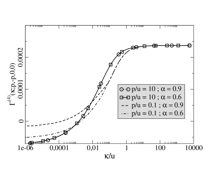
Figure 5: The function $\Gamma^{(4)}(\kappa,p,-p,0,0)$ (in units of $\Lambda$) for the values $p=10u$ and $p=u/10$ as a function of $\kappa/u$, for $\alpha=0.6$ and $\alpha=0.9$. The $\alpha$-dependence is largest when $p\simeq\kappa_{c}\simeq u/10$. When $p=10u\gg\kappa_{c}$, $\Gamma^{(4)}$ is independent of $\alpha$.

To study the $\alpha$-dependence of the 4-point function, it is convenient to separate $\Gamma^{(4)}_{12ll}(\kappa;p,-p,q,-q)$ into three contributions: that of the $s$-channel (see fig. 1), denoted by $\Gamma^{(4)[s]}$; the sum of the contributions of the $t$ and $u$-channels (see fig. 2), denoted by $\Gamma^{(4)[t+u]}$; finally the contribution of the 6-point function (see fig. 3), denoted as $\Gamma^{(4)[6]}$. That is, $\Gamma^{(4)[i]}$ denotes the contribution to the 4-point function obtained when only the channel $i$ is included in the calculation of $\Gamma^{(4)}$ according to eq. (II). There is an important difference between $\Gamma^{(4)[s]}$ and $\Gamma^{(4)[6]}$ on one side, and $\Gamma^{(4)[t+u]}$ on the other side: while $p$ flows through the loop in $\Gamma^{(4)[t+u]}$ (see fig. 2), in the other two cases it does not, so that the $p$-dependence of $\Gamma^{(4)[s]}$ and $\Gamma^{(4)[6]}$ comes entirely from the vertices. The latter are those of the initial ansatz $\tilde{\Gamma}^{(4)}$ and $\tilde{\Gamma}^{(6)}$, which depend on $p$ and $\alpha$ approximately only through the product $p\alpha$ (see paper I, sect. III and app. A). On the other hand, the $p$-dependence of $\Gamma^{(4)[t+u]}$ is mainly due to the explicit $p$-dependence of the loop in fig. 2, which is given by the ($\alpha$-independent) function $J_{d}^{(3)}(\kappa;p)$: Since $J_{d}^{(3)}(\kappa;p)$ is only important when $\kappa\mathrel{\hbox to0.0pt{\raise 2.20013pt\hbox{$>$}\hss}{\lower 2.20013pt\hbox{$\sim$}}}p$ (see fig. 9 in paper I), the contribution of the $t+u$ channels is non zero only in a region where the vertices in fig. 2 are essentially the ($p$ and $\alpha$ independent) LPA’ ones (see e.g. fig. 4). Then, one expects $\Gamma^{(4)[t+u]}_{12ll}(\kappa;p,-p,q,-q)$ to be almost independent of $\alpha$.

Fig. 5 shows that the total 4-point function $\Gamma^{(4)}(\kappa,p,-p,0,0)$ is in fact almost independent of $\alpha$ when $p=10u$, which indicates that the contributions of the $t$ and $u$ channels dominate for this value of $p$. The same holds for all values of $p$ much larger of much smaller than $u$. Only in the intermediate momentum region $p\sim\kappa_{c}\sim u/10$, is the variation with $\alpha$ important, which reflects the fact that in this intermediate range of momenta, the contributions of $\Gamma^{(4)[s]}$ and $\Gamma^{(4)[6]}$ are of the same order of magnitude as that of $\Gamma^{(4)[t+u]}$, as we shall verify later (see e.g. fig. 7 below, and the related discussion concerning the $\alpha$-dependence of $\Sigma_{NLO}(p)$).

III The self-energy and $\Delta\langle\varphi^{2}\rangle$ at NLO

We have now all the ingredients to calculate the self-energy at next-to-leading order. Recall that the physical self-energy at criticality is given by (see eq. (I.108))

$$\delta_{12}\Sigma(p)={1\over 2}\int_{0}^{\Lambda}d\kappa^{\prime}\int{d^{d}q\over(2\pi)^{d}}G^{2}(\kappa^{\prime};q)\partial_{\kappa^{\prime}}R_{\kappa^{\prime}}(q)\left(\Gamma^{(4)}_{12ll}(\kappa^{\prime};p,-p,q,-q)-\Gamma^{(4)}_{12ll}(\kappa^{\prime};0,0,q,-q)\right).$$

In order to get $\Sigma_{NLO}$, one needs to insert in the r.h.s. of eq. (III) the LO expression for the 4-point function $\Gamma^{(4)}_{12ll}(\kappa;p,-p,q,-q)$ which has been calculated in the previous section, and the LO propagator given by:

$$G^{-1}(\kappa;q)=q^{2}+\Sigma_{LO}(\kappa;q)+R_{\kappa}(q),$$ (35)

with $\Sigma_{LO}(\kappa;q)$ the LO expression of the self-energy, given by eq. (I.111).

III.1 Self-energy $\Sigma_{NLO}$

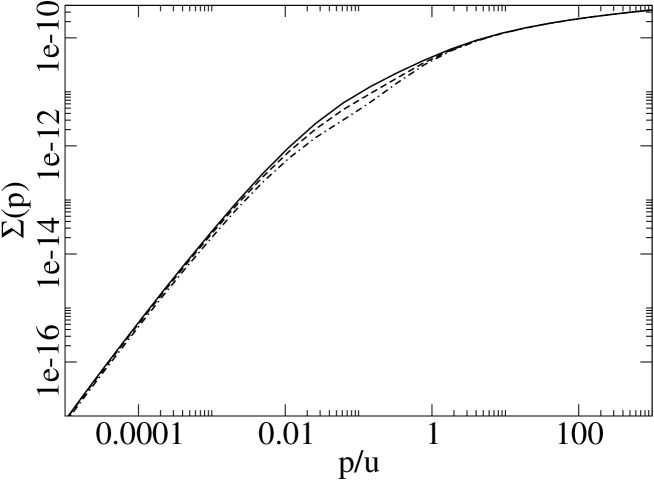
Figure 6: Self-energy at NLO (in units of $\Lambda^{2}$) as a function of $p/u$ for various values of $\alpha$: $\alpha=0.6$ (full line), $\alpha=0.75$ (dashed line) and $\alpha=0.9$ (dot-dashed line).

In this subsection, we present numerical results obtained for $d=3$ and $N=2$ in order to illustrate the main features of the self-energy. We shall use here the LO estimate of the 4-point function derived in the direct procedure. In the next subsection, we shall discuss results obtained with the improved procedure; we shall also present results for $N\neq 2$.

Fig. 6 displays the self-energy at NLO for various values of $\alpha$. It is to be compared with fig. 12 in paper I, for the LO behavior of $\Sigma(p)$. Note, however, that in paper I $\Sigma_{LO}$ is plotted as a function of $(\alpha p/u)$ in order to exhibit its approximate scaling property $\Sigma_{LO}(\alpha;p)\approx\hat{\Sigma}(\alpha p)$. Here $\Sigma_{NLO}$ is plotted as a function of $(p/u)$; as can be seen on fig. 6, $\Sigma_{NLO}$ depends much less on $\alpha$ than $\Sigma_{LO}$. In fact, both the IR and the UV regimes are nearly independent of $\alpha$. It is only in the intermediate momentum range ($p\sim\kappa_{c}$) that $\Sigma_{NLO}$ exhibits some dependence on $\alpha$.

At high momentum, one expects $\Sigma(p)$ to be given by perturbation theory, that is, one expects $\Sigma(p)\sim\ln(p/u)$. Recall that in paper I, we found that $\Sigma_{LO}(p)$ indeed behaves in this way, but the coefficient in front of the logarithm differed from that of perturbation theory by 7%. As we have discussed in paper I, perturbation theory is recovered exactly at high momenta when one performs iterations. In particular, the 2-loop result is exactly reproduced at NLO. We have verified that the coefficient in front of the logarithm in $\Sigma_{NLO}(p)$ at large $p$, is correctly obtained, to within the numerical accuracy with which it can be determined (about 0.5%).

In the IR regime, the power law behavior already reproduced in LO, $p^{2}+\Sigma_{LO}(p)\sim p^{2-\eta}$, is essentially not modified: however the numerical calculation is more involved in NLO, leading to a loss of accuracy that prevents us to determine the value of $\eta$ with any useful precision.

As was the case in LO, the $\alpha$-dependence of $\Sigma_{NLO}$ is intimately connected with its momentum dependence. Following the analysis that we did in sub-section II.4 to understand the variation of $\Gamma^{(4)}$ with $\alpha$, we split $\Sigma_{NLO}$ into three separate contributions: we define $\Sigma^{[s]}$, $\Sigma^{[t+u]}$ and $\Sigma^{[6]}$ as the contributions obtained, respectively, when only $\Gamma^{(4)[s]}$, $\Gamma^{(4)[t+u]}$ and $\Gamma^{(4)[6]}$ are included in the r.h.s. of eq. (III). The properties of the LO 4-point function discussed in the previous section imply that $\Sigma^{[s]}(\alpha;p)\approx\bar{\Sigma}^{[s]}(\alpha p)$, $\Sigma^{[6]}(\alpha;p)\approx\bar{\Sigma}^{[6]}(\alpha p)$ (i.e., the same dependence on $\alpha$ as $\Sigma_{LO}$ (see paper I, sect. IV A)), while $\Sigma^{[t+u]}$ is expected to be roughly independent of $\alpha$. These properties are well verified in our numerical calculations.

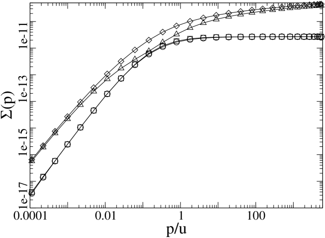
Figure 7: Self-energy $\Sigma_{NLO}(p)$ (in units of $\Lambda^{2}$) as a function of $p/u$ (triangle) at $\alpha=0.83$ and its three partial contributions $\Sigma^{[t+u]}$ (diamond), $-\Sigma^{[s]}$ (circle) and $-\Sigma^{[6]}$ (square).

The three contributions of the self-energy are shown in fig. 7 together with their sum $\Sigma_{NLO}$. While $\Sigma^{[t+u]}$ is positive, the two other contributions are negative. The latter property can be understood as follows: In calculating, say, $\Sigma^{[s]}$, one puts in eq. (III) only $\Gamma^{(4)[s]}$ which, in turn, is calculated with only the first term of eq. (II). In the latter, the flow is evaluated with the initial ansatz $\tilde{\Gamma}^{(4)}$ which, as can be seen in sect. III C of paper I, verifies, in all regions of momenta, $\tilde{\Gamma}^{(4)}(\kappa;p,-p,q,-q)>\tilde{\Gamma}^{(4)}(\kappa;0,0,q,-q)>0$. Since the integration over $\kappa^{\prime}$ that is needed to obtain $\Gamma^{(4)[s]}(\kappa)$ from eq. (II) runs from $\Lambda$ to $\kappa$, we have $\Gamma^{(4)[s]}(\kappa;p,-p,q,-q)<\Gamma^{(4)[s]}(\kappa;0,0,q,-q)$ so that the integrand in eq. (III) is negative, yielding eventually $\Sigma^{[s]}<0$. A similar analysis can be done for $\Sigma^{[6]}$. Fig. 7 shows that, as was the case for the 4-point function discussed in the previous section, the $t$ and $u$ channels dominate, except in the intermediate momentum region ($p\sim\kappa_{c}$) where the contributions of the three channels are of the same order of magnitude. This, together with the $\alpha$-dependence of $\Sigma^{[s]}$, $\Sigma^{[6]}$ and $\Sigma^{[t+u]}$ recalled in the previous paragraph, explains the behavior seen in fig. 6. Fig. 7 also reveals an interesting feature of the present approximation, for which we have no simple explanation: to within numerical accuracy, $\Sigma^{[s]}$ and $\Sigma^{[6]}$ appear indistinguishable. This property remains true for other values of $N$.

III.2 Calculation of $\Delta\langle\varphi^{2}\rangle$

We turn now to the calculation of the changes of the fluctuations of the field caused by the interactions:

$${\Delta\langle\phi_{i}^{2}\rangle\over N}=\int{{\rm d}^{3}p\over(2\pi)^{3}}\,\left({1\over p^{2}+\Sigma(p)}-{1\over p^{2}}\right)={1\over 2\pi^{2}}\int{dp\over p}\left[{p^{3}\over p^{2}+\Sigma(p)}-p\right].$$ (36)

As recalled in the introduction, and more thoroughly in paper I, this quantity is very sensitive to the intermediate momentum region and constitutes a stringent test of the calculation. In the following, we shall refer to the quantity in square brakets in eq. (36), multiplied by $1/(2\pi^{2})$, as to the integrand. Note that in the range of momenta where this integrand is significant (see e.g. fig. 8 below), $\Sigma(p)\ll p^{2}$, so that the integrand can be well approximated by $-\Sigma(p)/(2\pi^{2}\,p)$.

The results for $\Delta\langle\phi_{i}^{2}\rangle$ will be discussed in terms of the parameter

$$c\,\equiv-{256\pi^{3}\over\left(\zeta(3/2)\right)^{4/3}}\,{\Delta\langle\varphi_{i}^{2}\rangle\over Nu}.$$ (37)

The shift, caused by weak interactions, in the temperature of the Bose-Einstein transition of a dilute gas is directly proportional to $c$ club ; bigbec .

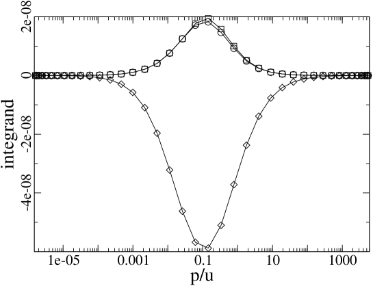
Figure 8: The three curves represent the integrand of eq. (36) (in units of $\Lambda$) calculated with only $\Sigma^{[t+u]}$ (diamonds), $\Sigma^{[s]}$ (circle) and $\Sigma^{[6]}$ (squares) contributions to the self-energy at NLO, respectively, as a function of $p/u$ (the points shown are those needed in the numerical calculation of the integral in eq. (36)). The plots correspond to $\alpha=0.83$ and $N=2$.

As we have seen in fig. 6, $\Sigma_{NLO}(p)$ is independent of the parameter $\alpha$ both at high and low momenta. However, in the crossover region ($p\sim\kappa_{c}$) which determines the value of $c$, $\Sigma_{NLO}(p)$ still depends on the value of $\alpha$. It follows that the value of the coefficient $c$ calculated with $\Sigma_{NLO}(p)$ still depends on $\alpha$. To understand better the $\alpha$-dependence of the NLO predictions, one can write the coefficient $c$ as the sum of three expressions, each of them containing only one of the three parts of the self-energy. The three contributions to the integrand yielding $c$ are displayed together in fig. 8. Because of the approximate scaling discussed above, both $\Sigma^{[s]}$ and $\Sigma^{[6]}$ contribute to $c$ with a term proportional to $\alpha$, while the contribution of $\Sigma^{[t+u]}$ is essentially independent of $\alpha$. This afine behavior of the NLO result for $c$ is indeed observed in fig. 9 below. The negative slope is due to the negative sign of $\Sigma^{(4)[s]}$ and $\Sigma^{(4)[6]}$.

The $\alpha$-dependence remains a source of uncertainty in the calculation of $c$. As can be seen on fig. 9, when we move from the LO calculation to the direct NLO, to the improved NLO, the dependence on $\alpha$ decreases, and so does the corresponding uncertainty in the calculated value of $c$. We regard the variation in the value of $c$ when $\alpha$ runs form $.6$ to $.9$ as a large overestimate of the uncertainty related to the choice of $\alpha$. In fact we can eliminate much of this uncertainty by following a procedure suggested by the results plotted in fig. 9: since the curves representing $c$ as a function of $\alpha$ have opposite slopes at LO and NLO, one can invoke a principle of fastest apparent convergence to choose as best estimate that given by the value of $\alpha$ for which the two curves cross: At this point indeed, the NLO correction vanishes. One thus obtains the value $c=1.44$ (the crossing point being at $\alpha=0.83)$ when we use the direct LO expression of the 4-point function, and $c=1.30$ with the improved LO (corresponding to $\alpha=0.77$). The improved NLO calculation is thus in remarkable agreement with the lattice data: $1.32\pm 0.02$ latt2 and $1.29\pm 0.05$ latt1 .

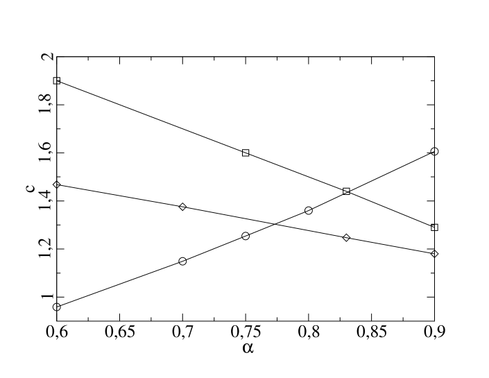
Figure 9: The coefficient $c$ as a function of $\alpha$ for $N=2$: LO (circles) from paper I, NLO direct (squares), NLO improved (diamonds).

We have also repeated our calculation for other values of $N$ for which results have been obtained with other techniques, either the lattice technique latt2 ; latt1 ; latt3 , or variationally improved 7-loops perturtbative calculations Kastening:2003iu . These results are summarized in table I and fig. 10 (other optimized perturbative calculations have also been recently performed, and are in agreement with those quoted here; see souza ; Kneur04 ). For small values ($N\mathrel{\hbox to0.0pt{\raise 2.20013pt\hbox{$<$}\hss}{\lower 2.20013pt\hbox{$\sim$}}}10$), our results fulfill all the numerical tests that we have described in this paper. For $N\leq 4$, where we can compare with other results, the values of $c$ obtained with the present improved NLO calculation are in excellent agreement with those obtained from lattice and 7-loops calculations.

What happens at large values of $N$ deserves a special discussion. As seen in fig. 10 the curve showing the improved leading order results extrapolates when $N\to\infty$ to a value that is about $4\%$ below the known exact result BigN . A direct calculation at very large values of $N$ is difficult in the present approach for numerical reasons: since the coefficient $c$ represents in effect an order $1/N$ correction (see BigN ), it is necessary to insure the cancellation of the large, order $N$, contributions to the self-energy, in order to extract the value of $c$. This is numerically demanding when $N\mathrel{\hbox to0.0pt{\raise 2.20013pt\hbox{$>$}\hss}{\lower 2.20013pt\hbox{$\sim$}}}100$. Fig. 10 also reveals an intriguing feature: there seems to be no natural way to reconcile the present results, and for this matter the results from lattice calculations or 7-loop calculations, with the calculation of the $1/N$ correction presented in ref. Arnold:2000ef : the dependence in $1/N$ of our results, be they obtained from the direct LO or the improved LO, appear to be incompatible with the slope predicted by the $1/N$ expansion.

$c$	$N=1$	$N=2$	$N=3$	$N=4$	$N=10$	$N=40$	$N=\infty$
lattice latt2		$1.32\pm 0.02$
lattice latt1		$1.29\pm 0.05$
lattice latt3	$1.09\pm 0.09$			$1.60\pm 0.10$
7-loops Kastening:2003iu	$1.07\pm 0.10$	$1.27\pm 0.10$	$1.43\pm 0.11$	$1.54\pm 0.11$
large $N$ BigN							$c=2.33$
this work	1.11	1.30	1.45	1.57	1.91	2.12

Table 1: Summary of available results for the coefficient $c$. The last line contains the results obtained in this work by using the improved LO approximation for the 4-point function.

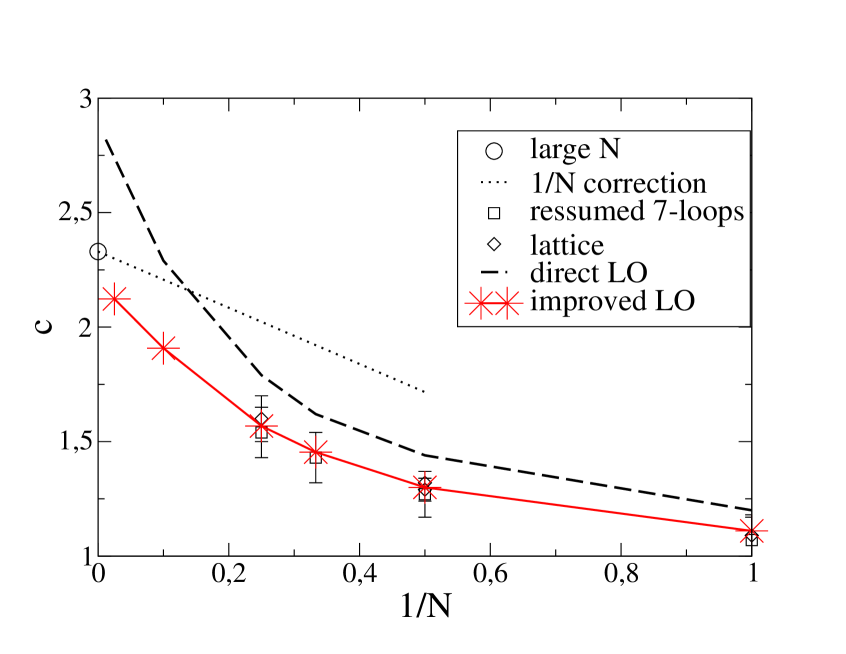
Figure 10: The coefficient $c$ (obtained with the fastest apparent convergence procedure) as a function of $1/N$. Our NLO results, are compared with results obtained with other methods: lattice latt2 ; latt1 ; latt3 (diamonds) and 7-loops perturbation theory Kastening:2003iu (squares), all of them with their corresponding error bars, together with the $N\to\infty$ result BigN (circle), and the extrapolation following the $1/N$ correction calculated in ref. Arnold:2000ef .

IV Summary and outlook

The quality of the results that we have obtained for the parameter $c$ that characterizes the shift in the transition temperature of the weakly repulsive Bose gas is encouraging. It demonstrates that the method that we have developed in order to solve the Non Perturbative Renormalisation Group is capable indeed to yield the full momentum dependence of the $n$-point functions, in physical regimes where other approximation schemes are limited.

It is of course difficult to quantify the size of the theoretical uncertainties in this approach. We have commented in the previous section about the source of uncertainty related to the choice of the parameter $\alpha$. A better estimate of the accuracy of the whole approximation scheme would be to perform one more iteration. However the numerical effort involved in the calculation of the relevant multidimensional integrals is non negligible, and furthermore the approximate equations that need to be solved in order to get the initial ansatz for the $n$-point functions become increasingly complicated (see for instance app. A). Thus it seems unrealistic to imagine doing a further iteration, going say to the next-to-next-to-leading order. What remains then, as a measure of the quality of the approximation scheme, is the direct comparison with results obtained by other, reliable, non perturbative methods, such as lattice calculations.

We have however started exploring an alternative approach which may have, among other features, the capability of yielding estimates for theoretical uncertainties. This approach builds on the present approximation scheme, but brings to it conceptual simplification. As we have seen when discussing results, both in paper I and in the present paper, the approximation ${\cal A}_{1}$ introduced in paper I is accurate in most situations encountered when solving the flow equations. This approximation assumes that the vertices in the r.h.s. of the flow equation are smooth functions of the momenta and exploits the fact that the loop momentum is bounded to neglect some of the momentum dependence. Once this is done, as shown in PLB , one can relate directly the higher $n$-point functions that arise in the r.h.s. of the flow equations to derivatives of the $n$-point function whose flow is being studied with respect to a constant background field. One then obtain closed equations. This method allows us to bypass both the approximation ${\cal A}_{3}$ needed for $n$-point functions of high order, and also the approximation ${\cal A}_{2}$ used to implement the decoupling of high momenta in the propagators. The price to pay is that the new equations are not only differential equations in the variable $\kappa$, but also partial differential equations with respect to the background field. However, they can be solved numerically, as will be demonstrated in a forthcoming publication BMWn .

Appendix A The initial ansatz for $\Gamma_{12llmm}^{(6)}(\kappa;p,-p,0,0,0,0)$

In order to obtain the explicit expression of the initial ansatz for $\Gamma^{(6)}$ we follow the same steps as in paper I, sect. III, when constructing the initial ansatz for $\Gamma^{(4)}$: We use the three approximations ${\cal A}_{1}$, ${\cal A}_{2}$ and ${\cal A}_{3}$ to get an approximate equation for the flow of $\Gamma^{(6)}$, which we then solve semi-analytically.

The exact flow equation for $\Gamma^{(6)}$ can be written in the following form, exhibiting three kinds of contributions:

$$\kappa\partial_{\kappa}\Gamma_{123456}^{(6)} = \mathop{\rm Tr}\nolimits G^{2}\kappa\partial_{\kappa}R_{\kappa}\left\{-\Gamma_{i12j}^{(4)}G\Gamma_{j34k}^{(4)}G\Gamma_{k56i}^{(4)}+\mathrm{44\,permutations}\right.$$ (38)

$$+ \left.\Gamma_{i1234j}^{(6)}G\Gamma_{j56i}^{(4)}+\mathrm{14\,permutations}-{1\over 2}\Gamma_{123456ii}^{(8)}\right\}.$$

We start by implementing approximations ${\cal A}_{1}$ and ${\cal A}_{2}$. To keep the discussion simple, we do so explicitly only for some typical terms of eq. (38). Take for example the following contribution involving the product of three $\Gamma^{(4)}$:

$$-\mathop{\rm Tr}\nolimits G^{2}\kappa\partial_{\kappa}R_{\kappa}\Gamma_{i12j}^{(4)}G\Gamma_{j34k}^{(4)}G\Gamma_{k56i}^{(4)}=-\int{d^{d}q\over(2\pi)^{d}}\kappa\partial_{\kappa}R_{\kappa}(q^{2})G(q^{2})\Gamma_{i12j}^{(4)}(q,p_{1},p_{2},-q-p_{1}-p_{2})$$

$$\times\;\;G((q+p_{1}+p_{2})^{2})\Gamma_{j34k}^{(4)}(q+p_{1}+p_{2},p_{3},p_{4},-q+p_{5}+p_{6})$$

$$\times\;\;G((q-p_{5}-p_{6})^{2})\Gamma_{k56i}^{(4)}(q-p_{5}-p_{6},p_{5},p_{6},-q).$$ (39)

After setting the external momenta to their values ($p_{3}=p_{4}=p_{5}=p_{6}=0,p_{2}=-p_{1}$), imposing $q=0$ in the vertices (approximation ${\cal A}_{1}$) and replacing $G(q+p)$ by $G_{LPA^{\prime}},\Theta(1-\alpha^{2}p^{2}/q^{2})$ (approximation ${\cal A}_{2}$), one gets:

$$-\mathop{\rm Tr}\nolimits G^{2}\kappa\partial_{\kappa}R_{\kappa}\Gamma_{i12j}^{(4)}G\Gamma_{j34k}^{(4)}G\Gamma_{k56i}^{(4)}=$$

$$-I_{d}^{(4)}(\kappa)\Gamma_{12ij}^{(4)}(p,-p,0,0)\Gamma_{34jk}^{(4)}(0,0,0,0)\Gamma_{56ki}^{(4)}(0,0,0,0),$$ (40)

where we have also made use of the symmetry of the bosonic $n$-point functions. A similar contribution corresponding to a different permutation reads:

$$-\mathop{\rm Tr}\nolimits G^{2}\kappa\partial_{\kappa}R_{\kappa}\Gamma_{i13j}^{(4)}G\Gamma_{j24k}^{(4)}G\Gamma_{k56i}^{(4)}=$$

$$-I_{d}^{(4)}(\kappa)\Theta(1-\alpha^{2}p^{2}/\kappa^{2})\Gamma_{1ji3}^{(4)}(p,-p,0,0)\Gamma_{j24k}^{(4)}(p,-p,0,0)\Gamma_{56ki}^{(4)}(0,0,0,0).$$ (41)

All 45 permutations containing three $\Gamma^{(4)}$ reduce either to the forms (A) or (A): those where both the external legs carrying the non-zero momenta ($p$ and $-p$) belong to the same $\Gamma^{(4)}$ are of the type (A), whereas those where the two legs with non-zero momenta belong to two different $\Gamma^{(4)}$ are of the type (A).

The second kind of contributions is that which involve one $\Gamma^{(4)}$ and one $\Gamma^{(6)}$. Among the 15 contributions of this kind, we have three different cases, depending on how the two external legs carrying non zero momenta are attached: both on $\Gamma^{(4)}$, both on $\Gamma^{(6)}$, one on $\Gamma^{(4)}$ and the other on $\Gamma^{(6)}$. We explicitly write here one contribution of the latter type:

$$\mathop{\rm Tr}\nolimits G^{2}\kappa\partial_{\kappa}R_{\kappa}\Gamma_{1345ij}^{(6)}G\Gamma_{26ji}^{(4)}=I_{d}^{(3)}(\kappa)\Theta(1-\alpha^{2}p^{2}/\kappa^{2})\Gamma_{1j4513}^{(6)}(p,-p,0,0,0,0)\Gamma_{j26i}^{(4)}(p,-p,0,0).$$

Finally, the third type of contributions is that which involves $\Gamma^{(8)}$:

$$-{1\over 2}\mathop{\rm Tr}\nolimits G^{2}\kappa\partial_{\kappa}R_{\kappa}\Gamma_{123456ij}^{(8)}=-{1\over 2}I_{d}^{(2)}(\kappa)\Gamma_{123456ii}^{(8)}(p,-p,0,0,0,0,0,0).$$ (43)

Observe that while all expressions in eqs. (A) and (A) are known (the explicit form of $\Gamma^{(4)}$ can be found in paper I, sect. IIIC), in the r.h.s. of eq. (A) appears the function $\Gamma^{(6)}$, the variable of the differential equation (38 ). Evaluating all the 15 permutations which includes this function $\Gamma^{(6)}$, one verifies that it appears either in the form $\Gamma^{(6)}(p,-p,0,0,0,0)$, or in the form $\Gamma^{(6)}(0,0,0,0,0,0)$. The latter being simply the (known) LPA’ expression (see paper I, sect. IIC), one ends up with a differential equation for the function $\Gamma^{(6)}(\kappa;p,-p,0,0,0,0)$. In order to solve it, one needs an initial ansatz for $\Gamma^{(8)}$ that appears in (43).

To get the latter, we follow approximation ${\cal A}_{3}$. Let us write the LPA’ equation corresponding to (38). This can be obtained by deriving three times with respect to $\rho$ the equation for the effective potential, and then setting $\rho=0$. One gets:

$$\partial_{\kappa}V^{\prime\prime\prime}(\rho=0) = \int{d^{d}q\over(2\pi)^{d}}\partial_{\kappa}R_{k}(q)G^{2}(q)\left\{-3(N+26)G^{2}(q)\left(V^{\prime\prime}(\rho=0)\right)^{3}\right.$$

$$+ \left.3(N+14)G(q)V^{\prime\prime\prime}(\rho=0)V^{\prime\prime}(\rho=0)-{N+6\over 2}V^{(4)}(\rho=0)\right\}.$$

Defining (see also paper I, sect. II C)

$$V^{(4)}(\rho=0)=l_{\kappa}=K_{d}^{-3}Z_{\kappa}^{4}\kappa^{8-3d}\hat{l}_{\kappa},$$ (45)

we transform eq. (A) into:

$$\kappa\partial_{\kappa}h_{\kappa}=-3(N+26)I_{d}^{(4)}(\kappa)g_{\kappa}^{3}+3(N+14)g_{\kappa}I_{d}^{(3)}(\kappa)h_{\kappa}-{1\over 2}(N+6)I_{d}^{(2)}(\kappa)l_{\kappa}.$$ (46)

On the other hand, as suggested by the large $N$ limit (see paper I, sect. II D), one expects that once approximation (${\cal A}_{2}$) is performed, the term containing $\Gamma^{(8)}$ to be proportional to the other ones, the coefficient depending only on $\kappa$. However, while in the case of the equation for $\Gamma^{(4)}$ the three contributions involving products of $\Gamma^{(4)}$ in eq. (II.1) where identical at zero external momenta (thus giving a unique proportional factor $F_{\kappa}$), here we have two different contributions (those with three $\Gamma^{(4)}$ and those with one $\Gamma^{(4)}$ and one $\Gamma^{(6)}$). Thus, the way the contribution of $\Gamma^{(8)}$ can be distributed over the other two is not unique. To remove the ambiguity, we distribute the various terms as they appear in the LPA’, eq. (46):

$$-{1\over 2}(N+6)I_{d}^{(2)}(\kappa)l_{\kappa}=3(N+26)I_{d}^{(4)}(\kappa)F^{\prime}_{\kappa}g_{\kappa}^{3}-3(N+14)I_{d}^{(3)}(\kappa)F_{\kappa}g_{\kappa}h_{\kappa},$$ (47)

where $F_{\kappa}$ is the function defined in eq. (I.44), while eq. (47) can be taken as the definition of $F^{\prime}_{\kappa}$. Using eqs. (I.42), (I.44) and (45), one then sets:

$$F^{\prime}_{\kappa}={(1+\hat{m}_{\kappa}^{2})^{2}\over\hat{g}_{\kappa}^{3}(N+26)}\left[{(N+14)(N+4)\over 2(N+8)}{\hat{h}_{\kappa}^{2}\over\hat{g}_{\kappa}}-{N+6\over 6}\hat{l}_{\kappa}\right].$$

The function $F^{\prime}_{\kappa}$ is shown in fig. 11.

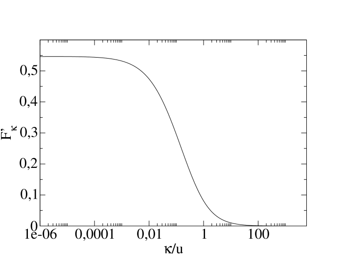
Figure 11: The function $F_{\kappa}^{\prime}$ as a function of $\kappa/u$.

We are now in the position to perform the approximation ${\cal A}_{3}$ in the flow equation of $\Gamma^{(6)}$, i.e., in eq. (38). This amounts to the replacement:

$$-{1\over 2}\mathop{\rm Tr}\nolimits\left\{\Gamma_{12345678}^{(8)}G^{2}\partial_{\kappa}R_{\kappa}\right\}\to\,\, \mathop{\rm Tr}\nolimits\left\{G^{2}\partial_{\kappa}R_{\kappa}\left(F^{\prime}_{\kappa}\Gamma_{i12j}^{(4)}G\Gamma_{j34k}^{(4)}G\Gamma_{k56i}^{(4)}+\mathrm{44\,permutations}\right.\right.$$

$$- \left.\left.3(N+14)F_{\kappa}\Gamma_{i1234j}^{(6)}G\Gamma_{j56k}^{(4)}+\mathrm{14\,permutations}\right)\right\}.$$

At this stage, we have all the ingredients to write, and solve, the (approximate) equation for $\Gamma^{(6)}$. After rewriting eq. (38) with the use of eq. (A), and evaluating all the terms as in eqs. (A), (A) and (A), one ends up with an ordinary differential equation where the dependent variable is $\Gamma^{(6)}(\kappa;p,-p,0,0,0,0)$. To write explicitly this equation it is useful to use the fact that $\Gamma^{(6)}_{123456}(p,-p,0,0,0,0)$ is completely symmetric under the exchange of indices 3, 4, 5 and 6. Then, one can make the decomposition:

$$\Gamma_{123456}^{(6)}(p,-p,0,0,0,0)=\Gamma^{(6)}_{a}\delta_{12}(\delta_{34}\delta_{56}+\delta_{35}\delta_{46}+\delta_{36}\delta_{45})$$ (50)

$$+ \Gamma^{(6)}_{b}\left[\delta_{24}(\delta_{13}\delta_{56}+\delta_{15}\delta_{36}+\delta_{16}\delta_{35})+\delta_{14}(\delta_{23}\delta_{56}+\delta_{25}\delta_{36}+\delta_{26}\delta_{35})\right.$$

$$+ \left.\delta_{13}\delta_{25}\delta_{46}+\delta_{13}\delta_{26}\delta_{45}+\delta_{15}\delta_{23}\delta_{46}+\delta_{15}\delta_{26}\delta_{43}+\delta_{16}\delta_{23}\delta_{45}+\delta_{16}\delta_{25}\delta_{34})\right],$$

Finally, taking the trace over the tensor indices, and doing a lengthy, but straightforward calculation, one gets:

$$\kappa\partial_{\kappa}\Gamma^{(6)}_{a} = (1-F_{\kappa})I_{d}^{(3)}(\kappa)\left\{g_{\kappa}\left[2(N+8)\Gamma^{(6)}_{a}+4\Gamma^{(6)}_{b}\right]\right.$$

$$+ \left.h_{\kappa}g_{\alpha p}\left[\left(N+6+{8\over N}\right)\left({g_{\kappa}\over g_{\alpha p}}\right)^{{N+2\over N+8}}-{8\over N}\left({g_{\kappa}\over g_{\alpha p}}\right)^{{2\over N+8}}\right]\right\}$$

$$- 3(1-F^{\prime}_{\kappa})I_{d}^{(4)}(\kappa)g^{2}_{\kappa}g_{\alpha p}\left\{(N+10+{16\over N})\left({g_{\kappa}\over g_{\alpha p}}\right)^{{N+2\over N+8}}-{16\over N}\left({g_{\kappa}\over g_{\alpha p}}\right)^{{2\over N+8}}\right\},$$

$$\kappa\partial_{\kappa}\Gamma^{(6)}_{b} = (1-F_{\kappa})I_{d}^{(3)}(\kappa)\left\{g_{\kappa}(N+16)\Gamma^{(6)}_{b}+2h_{\kappa}g_{\alpha p}\left({g_{\kappa}\over g_{\alpha p}}\right)^{{2\over N+8}}\right\}$$

$$- 12(1-F^{\prime}_{\kappa})I_{d}^{(4)}(\kappa)g^{2}_{\kappa}g_{\alpha p}\left({g_{\kappa}\over g_{\alpha p}}\right)^{{2\over N+8}},$$

when $\alpha p>\kappa$. When $\alpha p\leq\kappa$, one can show that the LPA’ expression for the 6-point vertex:

$$\Gamma_{12iijj}^{(6)}=\delta_{12}h_{\kappa}(N+2)(N+4)\;\;\;(\alpha p\leq\kappa),$$ (53)

is a solution of the equation that one gets. Then, as it is a first order differential equation in $\kappa$, the expression (53) is the solution for the case $\alpha p\leq\kappa$.

Returning to the case $\alpha p>\kappa$, one can diagonalize eqs. (A) and (A), the eigenvalues and eigenvectors being

$$\lambda_{a}=2(N+8) \hskip 28.45274pt\mathrm{with\,eigenvector}\,(1,0)$$

$$\lambda_{b}=N+16 \hskip 28.45274pt\mathrm{with\,eigenvector}\,(-4/N,1)$$ (54)

One thus can write:

$$\left(\begin{array}[]{c}\Gamma^{(6)}_{a}\\ \Gamma^{(6)}_{b}\end{array}\right)=a_{a}\left(\begin{array}[]{c}1\\ 0\end{array}\right)+a_{b}\left(\begin{array}[]{c}-4/N\\ 1\end{array}\right)$$ (61)

where $a_{a}$ verifies the equation:

$$\kappa\partial_{\kappa}a_{a}=(1-F_{\kappa})I_{d}^{(3)}(\kappa)2(N+8)g_{\kappa}a_{a}$$

$$+(1-F_{\kappa})I_{d}^{(3)}(\kappa)\left(N+6+{8\over N}\right)h_{\kappa}g_{\alpha p}\left({g_{\kappa}\over g_{\alpha p}}\right)^{{N+2\over N+8}}$$

$$-3(1-{F^{\prime}}_{\kappa})I_{d}^{(4)}(\kappa)\left(N+10+{16\over N}\right)\left(g_{\alpha p}\right)^{3}\left({g_{\kappa}\over g_{\alpha p}}\right)^{3{N+6\over N+8}}$$ (62)

while the equation for $a_{b}$ is simply the equation for $\Gamma^{(6)}_{b}$ (A).

Both equations (A) and (A) have the following form

$$\kappa\partial_{\kappa}\Gamma=\lambda I_{d}^{(3)}(\kappa)(1-F_{\kappa})g_{\kappa}\Gamma+\phi(\kappa)$$ (63)

its solution being

$$\Gamma(\kappa)=\Gamma(\alpha p)\left({g_{\kappa}\over g_{\alpha p}}\right)^{{\lambda\over N+8}}+\int_{\alpha p}^{\kappa}d\kappa^{\prime}\left({g_{\kappa}\over g_{\kappa^{\prime}}}\right)^{{\lambda\over N+8}}\phi(\kappa^{\prime})$$ (64)

Unfortunately we could not succeed to solve analytically the equation above, as we did for the initial ansatz for $\Gamma^{(4)}$; there, the key equation was (I.43), but we could not find a similar one here.

Imposing the continuity condition, in $\kappa=\alpha p$, dictated by eq. (53):

$$\Gamma^{(6)}_{a}(\alpha p)=\Gamma^{(6)}_{b}(\alpha p)=h_{\alpha p}$$ (65)

which gives

$$a_{a}(\alpha p) = \left(1+{4\over N}\right)h_{\alpha p}$$

$$a_{b}(\alpha p) = h_{\alpha p}$$ (66)

the solutions for $a_{a}(\kappa)$ and $a_{b}(\kappa)$ are

$$a_{a}(\kappa)=\left(1+{4\over N}\right)h_{\alpha p}\left({g_{\kappa}\over g_{\alpha p}}\right)^{2}$$

$$+ \int_{\log\alpha p/\Lambda}^{t}dt^{\prime}\left({g_{\kappa}\over g_{\kappa^{\prime}}}\right)^{2}\left\{(1-F_{\kappa})I_{d}^{(3)}(\kappa)(N+6+{8\over N})h_{\kappa}g_{\alpha p}\left({g_{\kappa}\over g_{\alpha p}}\right)^{{N+2\over N+8}}\right.$$

$$- \left.3(1-F^{\prime}_{\kappa})I_{d}^{(4)}(\kappa)(N+10+{16\over N})\left(g_{\alpha p}\right)^{3}\left({g_{\kappa}\over g_{\alpha p}}\right)^{3{N+6\over N+8}}\right\}$$

$$a_{b}(\kappa)=h_{\alpha p}\left({g_{\kappa}\over g_{\alpha p}}\right)^{{N+16\over N+8}}$$

$$+ \int_{\log\alpha p/\Lambda}^{t}dt^{\prime}\left({g_{\kappa}\over g_{\kappa}^{\prime}}\right)^{{N+16\over N+8}}\left\{2H_{\kappa}g_{\alpha p}\left({g_{\kappa}\over g_{\alpha p}}\right)^{{2\over N+8}}\right.$$

$$- \left.12(1-F^{\prime}_{\kappa})I_{d}^{(4)}(\kappa)g^{2}_{\kappa}g_{\alpha p}\left({g_{\kappa}\over g_{\alpha p}}\right)^{{2\over N+8}}\right\}$$

Finally, when $\kappa<\alpha p$, one has

$$\Gamma_{12iijj}^{(6)}(p,-p,0,0,0,0)=\delta_{12}N(N+2)a_{a}(\kappa)\;\;(\kappa<\alpha p).$$ (68)

Appendix B Products of functions $\tilde{\Gamma}^{(4)}$ in eq. (II)

B.1 The $s$ and $t$-channel contributions

In this appendix we obtain explicit expressions for the products of functions $\tilde{\Gamma}^{(4)}$ that appear in the r.h.s. of eq. (II), where $\tilde{\Gamma}^{(4)}$ is the initial ansatz for the 4-point function. All the needed expressions for the 4-point fucntions that are needed here are those for $\tilde{\Gamma}^{(4)}(p_{1},p_{2},0,-p_{1}-p_{2})$ that can be found in paper I, sect. III B.

1) The $s$-channel contribution

Here we consider the product $\tilde{\Gamma}^{(4)}_{12ij}(\kappa;p,-p,0,0)\tilde{\Gamma}^{(4)}_{llij}(\kappa;q,-q,0,0)$, where, because of the regulator, $q<\kappa$. There are two regions to examine:

a) $\alpha p<\kappa$

Both 4-point functions are in the region (a) of paper I, sect. III C. After a simple calculation one gets:

$$\tilde{\Gamma}^{(4)}_{12ij}(p,-p,0,0)\tilde{\Gamma}^{(4)}_{llij}(q,-q,0,0)=(N+2)^{2}g_{\kappa}^{2}\delta_{12}.$$ (69)

b) $\alpha p>\kappa$

Here, while $\tilde{\Gamma}^{(4)}_{llij}(q,-q,0,0)$ is still in region (a), the other vertex is in region (b) of paper I, sect. III C. In this case one gets:

$$\tilde{\Gamma}^{(4)}_{12ij}(p,-p,0,0)\tilde{\Gamma}^{(4)}_{llij}(q,-q,0,0)=(N+2)^{2}g_{\kappa}g_{\alpha p}\left({g_{\kappa}\over g_{\alpha p}}\right)^{{N+2\over N+8}}\delta_{12}.$$ (70)

2) The $t$-channel contribution

Here we consider the product $\tilde{\Gamma}^{(4)}_{12ij}(p,-p,0,0)\tilde{\Gamma}^{(4)}_{llij}(q,-q,0,0)$. As $q<\kappa$ and $\alpha<1$ (and thus $\alpha q\leq\kappa$), one has two cases to study: $p>|p+q|$ and $|p+q|>p$.

A) $p>|p+q|$

In paper I, sect. III B, we assumed $p_{1}>p_{2}>|p_{1}+p_{2}|$. Using the symmetry of the bosonic $n$-point functions, we can conveniently rewrite the product as

$$\tilde{\Gamma}^{(4)}_{1lij}(p,q,0,-p-q)\tilde{\Gamma}^{(4)}_{2lij}(-p,-q,0,p+q)=\tilde{\Gamma}^{(4)}_{1jil}(p,-p-q,0,q)\tilde{\Gamma}^{(4)}_{2jil}(p,-p-q,0,q),$$

and the expressions of the vertices to consider are those of either regions (a), (b), or (c) of paper I, sect. III B, depending on the value of $\kappa$ (region (d) never enters, because $q<\kappa$):

a) $\kappa>\alpha p$

The two vertices are in region (a) of paper I, sect. III B. The product is simply:

$$\tilde{\Gamma}^{(4)}_{1jil}(p,-p-q,0,q)\tilde{\Gamma}^{(4)}_{2jil}(p,-p-q,0,q)=3(N+2)g^{2}_{\kappa}\delta_{12}.$$ (72)

b) $\alpha p>\kappa>\alpha|p+q|$

Now, both vertices are in region (b) of paper I, sect. III B. A lengthy but straigtforward calulation yields:

$$\tilde{\Gamma}^{(4)}_{1jil}(p,-p-q,0,q)\tilde{\Gamma}^{(4)}_{2jil}(p,-p-q,0,q)=$$

$$g^{2}_{\alpha p}{N+2\over N^{2}+4N+20}\left\{\left({3\over 2}N^{2}+6N+30+{N+14\over 2}\sqrt{N^{2}+4N+20}\right)\left({g_{\kappa}\over g_{\alpha p}}\right)^{{2\lambda_{+}\over N+8}}\right.$$

$$\left.+\left({3\over 2}N^{2}+6N+30-{N+14\over 2}\sqrt{N^{2}+4N+20}\right)\left({g_{\kappa}\over g_{\alpha p}}\right)^{{2\lambda_{-}\over N+8}}\right\}\delta_{12}$$

c) $\alpha|p+q|>\kappa$

Both vertices are now in region (c) of paper I, sect. III B. After another straigtforward calulation one obtains:

$$\tilde{\Gamma}^{(4)}_{1jil}(p,-p-q,0,q)\tilde{\Gamma}^{(4)}_{2jil}(p,-p-q,0,q)=$$

$$\left\{N\left(b^{+}_{\alpha|p+q|}\left({g_{\kappa}\over g_{\alpha|p+q|}}\right)^{{\lambda_{1}\over N+8}}\right.+b^{-}_{\alpha|p+q|}\left({g_{\kappa}\over g_{\alpha|p+q|}}\right)^{{\lambda_{2}\over N+8}}\right)^{2}$$

$$-2Nb^{-}_{\alpha|p+q|}\left({g_{\kappa}\over g_{\alpha|p+q|}}\right)^{{\lambda_{2}\over N+8}}$$

$$\left(b^{+}_{\alpha|p+q|}\left({g_{\kappa}\over g_{\alpha|p+q|}}\right)^{{\lambda_{1}\over N+8}}+b^{-}_{\alpha|p+q|}\left({g_{\kappa}\over g_{\alpha|p+q|}}\right)^{{\lambda_{2}\over N+8}}\right)$$

$$\left.+{N^{2}\over 2}(N+1)b^{-}_{{}^{2}(\alpha|p+q|}\left({g_{\kappa}\over g_{\alpha|p+q|}}\right)^{2{\lambda_{2}\over N+8}}+2(N-1){\Gamma^{C}}^{2}_{\alpha|p+q|}\right\}\delta_{12}$$

where $b^{+}_{\alpha|p+q|}$, $b^{-}_{\alpha|p+q|}$ and $\Gamma^{C}_{\alpha|p+q|}$ follow from eqs. (I.92) and (I.93) respectively.

B) $p\leq|p+q|$

In this case, we reorder momenta and indices as:

$$\tilde{\Gamma}^{(4)}_{1lij}(p,q,0,-p-q)\tilde{\Gamma}^{(4)}_{2lij}(-p,-q,0,p+q)=\tilde{\Gamma}^{(4)}_{j1il}(-p-q,p,0,q)\tilde{\Gamma}^{(4)}_{j2il}(-p-q,p,0,q).$$ (75)

Similarly as in previous case (A) one has three regions, $\kappa>\alpha|p+q|$, $\alpha|p+q|>\kappa>\alpha p$ and $\alpha p>\kappa$. For each region the result is the same as those in eqs. (72), (B.1) and (B.1), but exchanging $p$ with $|p+q|$.

- [1] J. P. Blaizot, R. Mendez Galain and N. Wschebor, Non-Perturbative Renormalisation Group equations and momentum dependence of -point functions (I), hep-th/0512317, to be submitted for publication.
- [2] C.Wetterich, Phys. Lett., B301, 90 (1993).
- [3] U.Ellwanger, Z.Phys., C58, 619 (1993).
- [4] N. Tetradis and C. Wetterich, Nucl. Phys. B 422, 541 (1994).
- [5] T.R.Morris, Int. J. Mod. Phys., A9, 2411 (1994).
- [6] T.R.Morris, Phys. Lett. B329, 241 (1994).
- [7] J. Berges, N. Tetradis and C. Wetterich, Phys. Rept. 363, 223–386 (2002).
- [8] C. Bagnuls and C. Bervillier, Phys. Rept. 348, 91 (2001).
- [9] L. Canet and B. Delamotte, cond-matt/0412205.
- [10] G. Baym, J.-P. Blaizot, M. Holzmann, F. Laloë, and D. Vautherin, Phys. Rev. Lett. 83, 1703 (1999).
- [11] J. P. Blaizot, R. Mendez Galain and N. Wschebor, Europhys. Lett., 72 (5), 705-711 (2005).
- [12] D.Litim, Phys. Lett. B486, 92 (2000); Phys. Rev. D64, 105007 (2001); Nucl. Phys. B631, 128 (2002); Int.J.Mod.Phys. A16, 2081 (2001).
- [13] J. P. Blaizot, R. Mendez Galain and N. Wschebor, Phys. Lett. B632, 571-578 (2006).
- [14] J. P. Blaizot, R. Mendez Galain and N. Wschebor, Non-Perturbative Renormalisation Group calculation of the self-energy of a scalar field, in preparation.
- [15] G. Baym, J.-P. Blaizot, M. Holzmann, F. Laloë, and D. Vautherin, Eur. Phys. J. B24, 107 (2001).
- [16] P. Arnold and G. Moore, Phys. Rev. Lett. 87, 120401 (2001).
- [17] V.A. Kashurnikov, N. V. Prokof’ev, and B. V. Svistunov, Phys. Rev. Lett. 87, 120402 (2001).
- [18] X. Sun, Phys. Rev. E67, 066702 (2003).
- [19] B. M. Kastening, Phys. Rev. A 69, 043613 (2004).
- [20] F. de Souza Cruz, M.B. Pinto, and R.O. Ramos, Phys. Rev. B64, 014515 (2001); Phys. Rev. A 65, 053613 (2002).
- [21] J.-L. Kneur, A. Neveu, M. B. Pinto, Phys. Rev. A69, 053624 (2004).
- [22] G. Baym, J-P. Blaizot and J. Zinn-Justin, Europhys. Lett. 49, 150 (2000).
- [23] P. Arnold and B. Tomasik, Phys. Rev. A 62, 063604 (2000).
- [24] S.Ledowski, N. Hasslmann and P. Kopietz, Phys. Rev. A 69, 061601(R) (2004)