Bosonization of non-relativistic fermions on a circle: Tomonaga’s problem revisited

Abstract:

We use the recently developed tools for an exact bosonization of a finite number $N$ of non-relativistic fermions to discuss the classic Tomonaga problem. In the case of noninteracting fermions, the bosonized hamiltonian naturally splits into an O$(N)$ piece and an O$(1)$ piece. We show that in the large-$N$ and low-energy limit, the O$(N)$ piece in the hamiltonian describes a massless relativistic boson, while the O$(1)$ piece gives rise to cubic self-interactions of the boson. At finite $N$ and high energies, the low-energy effective description breaks down and the exact bosonized hamiltonian must be used. We also comment on the connection between the Tomonaga problem and pure Yang-Mills theory on a cylinder. In the dual context of baby universes and multiple black holes in string theory, we point out that the O$(N)$ piece in our bosonized hamiltonian provides a simple understanding of the origin of two different kinds of nonperturbative O$(e^{-N})$ corrections to the black hole partition function.

1 Introduction

In a recent work [1] we have discussed an exact bosonization of a finite number $N$ of non-relativistic fermions. The tools developed there have many potential applications to several areas of physics. An example is the half-BPS sector of ${\cal N}=4$ super Yang-Mills theory and its holographic dual string theory in $AdS_{5}\times S^{5}$  space-time, some aspects of which were discussed in [1] and more recently in greater detail in [2]. In the present work we will discuss application of our exact bosonization to the classic Tomonaga problem [3] of non-relativistic fermions on a circle.

Historically, the Tomonaga problem has played an important role in the development of tools for treating a system of large number of fermions interacting with long-range forces like Coulomb force, which is an essential problem one encounters in condensed matter systems. In the toy model of a $1$-dimensional system of non-relativistic fermions, Tomonaga was the first to show that interactions can mediate new collective dynamical degrees of freedom, which are quantized as bosons. The essential idea was the observation that a long-range (in real space) force like Coulomb interaction becomes short range in momentum space, so particle-hole pairs in a low-energy band around fermi surface (which consists of just two points in $1$-dimension) do not get “scattered out” of the band. As a result, the interacting ground state, as well as excited states with low excitation energy compared to the fermi energy, involve only particle-hole pairs in a small band around the fermi surface. For a large number of fermions, there is a finite band around the fermi surface in which the excited states satisfy this requirement. In his work, Tomonaga laid down precise criteria for the collective boson low-energy approximation to work, and showed that when his criteria are met, both the free as well as the interacting fermion systems can be described by a system of free bosons, under a suitable approximation, for a system of large number of fermions.

In the present work, we will apply our exact bosonization tools to the Tomonaga problem. The states of our bosonized theory are multiparticle states of a system of free bosons, each of which can be in any of the first $N$ levels of a harmonic oscillator, where $N$ is the number of fermions. These states diagonalize the non-interacting part of the fermion hamiltonian exactly. We will show that the standard effective low-energy theory for appropriate Fourier modes of the spatial fermion density operator can be derived from this bosonized theory. We will see that the conditions under which this can be done are precisely the ones required by Tomonaga for his approximations to work. However, for the non-interacting case our exact bosonization is applicable even outside the regime of validity of the low-energy approximation.

The organization of this paper is as follows. In Sec 2 we summarize the work of [1] on the exact bosonization of a finite number $N$ of nonrelativistic fermions. The presentation here is different and simpler, though completely equivalent to that in [1]. The merit of this presentation is that it makes the bosonization rules simpler and graphical, making applications of these rules very easy. In Sec 3 we derive the bosonized hamiltonian for a system of $N$ non-relativistic fermions on a circle. The free fermion system has a degenerate spectrum, so we need to do further work before applying the bosonization rules of Sec 2. After explaining how to take care of the degeneracy, we derive the bosonized form of the hamiltonian. The nontrivial part of the bosonized hamiltonian naturally splits into a sum of a large, O$(N)$, piece and a small, O$(1)$ piece. We show that ignoring the latter corresponds to the relativistic boson approximation of Tomonaga. We do this by computing the partition function of the O$(N)$ piece in the hamiltonian, which reduces at large $N$ to that of a relativistic boson. The O$(1)$ piece gives rise to a cubic self-interaction of this boson. This is shown in Sec 4 where we derive the effective low-energy cubic hamiltonian for these self-interactions. Extension beyond low-energy approximation is discussed in Sec 5. Interacting fermion case is discussed in Sec 6. Connection of the Tomonaga problem with Yang-Mills theory on a two-dimensional cylinder is discussed in Sec 7. We end with a summary and some comments in Sec 8. Details of some computations described in the text are given in Appendices A, B and C. In Appendix D we discuss possible extension of our bosonization techniques to higher dimensions.

2 Review of exact bosonization

In this section we will review the techniques developed in [1] for an exact operator bosonization of a finite number of nonrelativistic fermions. The discussion here is somewhat different from that in [1]. Here, we will derive the first bosonization of [1] using somewhat simpler arguments, considerably simplifying the presentation and the formulae in the process. Moreover, the present derivation of bosonization rules is more intuitive, making its applications technically easier.

Consider a system of $N$ fermions each of which can occupy a state in an infinite-dimensional Hilbert space ${\cal H}_{f}$. Suppose there is a countable basis of ${\cal H}_{f}:\{|m\rangle,m=0,1,\cdots,\infty\}$. For example, this could be the eigenbasis of a single-particle hamiltonian, $\hat{h}|m\rangle={\cal E}(m)|m\rangle$, although other choices of basis would do equally well, as long as it is a countable basis. In the second quantized notation we introduce creation (annihilation) operators $\psi^{\dagger}_{m}$ ($\psi_{m}$) which create (destroy) particles in the state $|m\rangle$. These satisfy the anticommutation relations

$$\{\psi_{m},\psi^{\dagger}_{n}\}=\delta_{mn}$$ (1)

The $N$-fermion states are given by (linear combinations of)

$$|f_{1},\cdots,f_{N}\rangle=\psi^{\dagger}_{f_{1}}\psi^{\dagger}_{f_{2}}\cdots\psi^{\dagger}_{f_{N}}|0\rangle_{F}$$ (2)

where $f_{m}$ are arbitrary integers satisfying $0\leq f_{1}<f_{2}<\cdots<f_{N}$, and $|0\rangle_{F}$ is the usual Fock vacuum annihilated by $\psi_{m},m=0,1,\cdots,\infty$.

It is clear that one can span the entire space of $N$-fermion states, starting from a given state $|f_{1},\cdots,f_{N}\rangle$, by repeated application of the fermion bilinear operators

$$\Phi_{mn}=\psi^{\dagger}_{m}\,\psi_{n}$$ (3)

However, the problem with these bosonic operators is that they are not independent; this is reflected in the W_∞ algebra that they satisfy,

$$[\Phi_{mn},\Phi_{m^{\prime}n^{\prime}}]=\delta_{m^{\prime}n}\Phi_{mn^{\prime}}-\delta_{mn^{\prime}}\Phi_{m^{\prime}n}.$$ (4)

This is the operator version of the noncommutative constraint $u*u=u$ that the Wigner distribution $u$ satisfies in the exact path-integral bosonization carried out in [5].

A new set of unconstrained bosonic operators was introduced in [1], $N$ of them for $N$ fermions. In effect, this set of bosonic operators provides the independent degrees of freedom in terms of which the above constraint is solved. Let us denote these operators by $\sigma_{k},~{}k=1,2,\cdots,N$ and their conjugates, $\sigma^{\dagger}_{k},~{}k=1,2,\cdots,N$. As we shall see shortly, these operators will turn out to be identical to the $\sigma_{k}$’s used in [1]. The action of $\sigma^{\dagger}_{k}$ on a given fermion state $|f_{1},\cdots,f_{N}\rangle$ is rather simple. It just takes each of the fermions in the top $k$ occupied levels up by one step, as illustrated in Figure 1. One starts from the fermion in the topmost occupied level, $f_{N}$, and moves it up by one step to $(f_{N}+1)$, then the one below it up by one step, etc proceeding in this order, all the way down to the $k$th fermion from top, which is occupying the level $f_{N-k+1}$ and is taken to the level $(f_{N-k+1}+1)$. For the conjugate operation, $\sigma_{k}$, one takes fermions in the top occupied $k$ levels down by one step, reversing the order of the moves. Thus, one starts by moving the fermion at the level $f_{N-k+1}$ to the next level below at $(f_{N-k+1}-1)$, and so on. Clearly, in this case the answer is nonzero only if the $(k+1)$th fermion from the top is not occupying the level immediately below the $k$th fermion , i.e. only if $(f_{N-k+1}-f_{N-k}-1)>0$. If $k=N$ this condition must be replaced by $f_{1}>0$.

Figure 1: The action of $\sigma_{k}^{\dagger}$.

These operations are necessary and sufficient to move to any desired fermion state starting from a given state. This can be argued as follows. First, consider the following operator, $\sigma_{k-1}~{}\sigma^{\dagger}_{k}$. Acting on an arbitrary fermion state, the first factor takes top $k$ fermions up by one level; this is followed by bringing the top $(k-1)$ fermions down by one level. The net effect is that only the $k$th fermion from top is moved up by one level. In other words, $\sigma_{k-1}~{}\sigma^{\dagger}_{k}=\psi^{\dagger}_{f_{N-k+1}+1}~{}\psi_{f_{N-k+1}}=\Phi_{{f_{N-k+1}+1},f_{N-k+1}}$. In this way, by composing together different $\sigma_{k}$ operations we can move individual fermions around. Clearly, all the $N$ $\sigma_{k}$ operations are necessary in order to move each of the $N$ fermions indvidually. It is easy to see that by applying sufficient number of such fermion bilinears one can move to any desired fermion state starting from a given state.

It follows from the definition of $\sigma^{\dagger}_{k},~{}\sigma_{k}$ operators that they satisfy the following relations:

$$\sigma_{k}~{}\sigma^{\dagger}_{k}=1,~{}~{}\sigma^{\dagger}_{k}~{}\sigma_{k}=\theta(r_{k}-1),~{}~{}[\sigma_{l},\sigma^{\dagger}_{k}]=0,~{}~{}l\neq k,$$ (5)

where $(f_{N-k+1}-f_{N-k}-1)\equiv r_{k}$ and $\theta(m)=1$ if $m\geq 0$, otherwise it vanishes. Moreover, all the $\sigma_{k}$’s annihilate the Fermi vacuum.

Consider now a system of bosons each of which can occupy a state in an $N$-dimensional Hilbert space ${\cal H}_{N}$. Suppose we choose a basis $\{|k\rangle,~{}k=1,\cdots,N\}$ of ${\cal H}_{N}$. In the second quantized notation we introduce creation (annihilation) operators $a^{\dagger}_{k}$ ($a_{k}$) which create (destroy) particles in the state $|k\rangle$. These satisfy the commutation relations

$$[a_{k},a^{\dagger}_{l}]=\delta_{kl},\quad k,l=1,\cdots,N$$ (6)

A state of this bosonic system is given by (a linear combination of)

$$|r_{1},\cdots,r_{N}\rangle=\frac{(a_{1}^{\dagger})^{r_{1}}\cdots(a_{N}^{\dagger})^{r_{N}}}{\sqrt{r_{1}!\cdots r_{N}!}}|0\rangle$$ (7)

It can be easily verified that equations (5) are satisfied if we make the following identifications

$$\sigma_{k} = \frac{1}{\sqrt{a^{\dagger}_{k}a_{k}+1}}a_{k},$$

$$\sigma^{\dagger}_{k} = a^{\dagger}_{k}\frac{1}{\sqrt{a^{\dagger}_{k}a_{k}+1}},$$ (8)

together with the map

$$r_{k} = f_{N-k+1}-f_{N-k}-1,\quad\quad k=1,\,2,\,\cdots\,N-1$$

$$r_{N} = f_{1}.$$ (9)

This identification is consistent with the Fermi vacuum being the ground state of the bosonic system. The map (9) first appeared in [6]. The first of these arises from the identification (8) of $\sigma_{k}$’s in terms of the oscillator modes, while the second follows from the fact that $\sigma_{N}$ annihilates any state in which $f_{1}$ vanishes.

Using the above bosonization formulae, any fermion bilinear operator can be expressed in terms of the bosons. For example, the hamiltonian can be rewritten as follows. Let ${\cal E}(m),~{}m=0,1,2,\cdots$ be the exact single-particle spectrum of the fermions (assumed noninteracting). Then, the hamiltonian is given by

$$H=\sum_{m=0}^{\infty}{\cal E}(m)~{}\psi^{\dagger}_{m}~{}\psi_{m}.$$ (10)

Its eigenvalues are $E=\sum_{k=1}^{N}{\cal E}(f_{k})$. Using $f_{k}=\sum_{i=N-k+1}^{N}r_{i}+k-1$, which is easily derived from (9), these can be rewritten in terms of the bosonic occupation numbers, $E=\sum_{k=1}^{N}{\cal E}(\sum_{i=N-k+1}^{N}r_{i}+k-1)$. These are the eigenvalues of the bosonic hamiltonian

$$H=\sum_{k=1}^{N}{\cal E}(\hat{n}_{k}),\quad\hat{n}_{k}\equiv\sum_{i=k}^{N}a^{\dagger}_{i}a_{i}+N-k$$ (11)

This bosonic hamiltonian is, of course, completely equivalent to the fermionic hamiltonian we started with.

We end this section with the remark that our bosonization technique does not depend on any specific choice of fermion hamiltonian and can be applied to various problems like $c=1$, half-BPS sector of ${\cal N}=4$ super Yang-Mills theory [2], etc.

3 Free non-relativistic fermions on a circle - Large $N$ limit

In this and the next section, we will discuss the theory obtained by bosonization of the noninteracting part of the fermion hamiltonian. The case of interacting fermions will be taken up in Sec 5. In the second quantized langauge, we may write the free part as

$$H_{\rm free}=-\frac{\hbar^{2}}{2m}\int_{0}^{L}dx\ \chi^{\dagger}(x)\partial_{x}^{2}\chi(x).$$ (12)

Here $L$ is the size of the circle and $m$ is the mass of each fermion. In terms of the fourier modes, $\chi_{\pm n}\equiv\int_{0}^{L}\frac{dx}{\sqrt{L}}\ e^{\mp 2\pi inx/L}\ \chi(x)$, where $n=0,1,2,\cdots$, we have

$$H_{\rm free}=\omega\hbar\sum_{n=1}^{\infty}n^{2}(\chi^{\dagger}_{+n}\chi_{+n}+\chi^{\dagger}_{-n}\chi_{-n}),\ \ \omega\equiv\frac{2\pi^{2}\hbar}{mL^{2}}.$$ (13)

Note that the zero mode, $\chi_{0}$, does not enter in the expression for the hamiltonian. The fermion modes satisfy the canonical anti-commutation relations,

$$\{\chi_{\pm n},~{}\chi^{\dagger}_{\pm l}\}=\delta_{nl},$$ (14)

all other anticommutators vanish.

3.1 The bosonized hamiltonian

The bosonization rules that we have developed in Sec. 2 cannot be applied directly to this hamiltonian because of the degeneracy between $\pm n$ modes. To get around this difficulty, we will change the hamiltonian by replacing $n^{2}$ in the sum in (13) by $(n+\epsilon)^{2}$, where $\epsilon$ is a small positive real number. The original problem will be recovered by setting $\epsilon$ to zero after bosonization is done . For a non-zero positive value of epsilon , the energy of the mode for $+n$ is higher than that for $-n$. So the spectrum is now non-degenerate and looks like that shown in Figure 2.

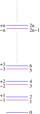
Figure 2: The spectrum with a specified ordering for degenerate levels.

The next step is to redefine $\chi_{0}\equiv\psi_{0}$, $\chi_{-n}\equiv\psi_{2n-1}$ and $\chi_{+n}\equiv\psi_{2n}$, $n\neq 0$. The hamiltonian (13) can then be rewritten as

$$H_{\rm free}=\frac{\omega\hbar}{4}\sum_{n=0}^{\infty}[n+e(n)+(-1)^{n}2\epsilon]^{2}\psi^{\dagger}_{n}\psi_{n}.$$ (15)

Here $e(n)$ vanishes for even $n$ and equals unity for odd $n$, i.e.

$$e(n)\equiv\frac{1}{2}(1-(-1)^{n}).$$ (16)

Note that the zero mode piece in (15) vanishes when $\epsilon$ is set to zero. Since this hamiltonian has the generic form (10), its bozonied version can be readily written down using (11). Setting $\epsilon$ to zero in the final expression, we get

$$H_{\rm free}=\frac{\omega\hbar}{4}\sum_{k=1}^{N}\biggl{(}\hat{n}_{k}+e(\hat{n}_{k})\biggr{)}^{2},\quad\hat{n}_{k}\equiv\sum_{i=k}^{N}a^{\dagger}_{i}a_{i}+N-k$$ (17)

This is the final form of the bosonized hamiltonian for free non-relativistic fermions on a circle.

3.2 The relativistic boson approximation

In his work, Tomonaga showed that for a large number of non-interacting fermions, small fluctuations of the fermi surface are described by a free relativistic boson. Our bosonic states diagonalize $H_{\rm free}$ exactly, even for highly excited states. So it is not surprising that the relativistic boson is not manifest in our bosonization. However, we should be able to recover the relativistic boson from it in the low-energy, low-momentum sector of the large-$N$ limit. In the remainder of this subsection we will explain how that happens.

The first step is to extract the part of $H_{\rm free}$ which describes low-energy and low-momentum fluctuations of the two fermi points. To this end, we note that $H_{\rm free}$ can be rewritten as follows:

$$H_{\rm free}=H_{F}+H_{0}+H_{1},$$ (18)

where $H_{F}=\frac{\omega\hbar}{4}\sum_{k=1}^{N}(N-k+e(N-k))^{2}$ is the energy of the fermi vacuum and

$$H_{0} = \frac{\hbar\omega N}{2}\biggl{(}\sum_{k=1}^{N}k~{}a^{\dagger}_{k}a_{k}+\hat{\nu}\biggr{)},$$ (19)

$$H_{1} = \frac{\hbar\omega}{4}\sum_{k=1}^{N}\biggl{[}\biggl{(}-k^{2}+(-1)^{N}e(k)\biggr{)}a^{\dagger}_{k}a_{k}-2\biggl{(}k(-1)^{N-k}+e(N-k)\biggr{)}e(\sum_{i=k}^{N}a^{\dagger}_{i}a_{i})$$ (20)

$$~{}~{}~{}~{}~{}~{}+\biggl{(}\sum_{i=k}^{N}a^{\dagger}_{i}a_{i}+(-1)^{N-k}e(\sum_{i=k}^{N}a^{\dagger}_{i}a_{i})\biggr{)}^{2}\biggr{]}$$

Details of the manipulations required to cast the hamiltonian in this form suitable for perturbative treatment are given in Appendix A. In (19), $\hat{\nu}=N_{-}-N_{-F}$ is the operator which measures change in the number of negative momentum fermions in the given state compared to the fermi vacuum. In terms of bosonic occupation number operators, the number of negative momentum fermions, $N_{-}$, is given by the expression

$$N_{-}=\sum_{k=1}^{N}e(\hat{n}_{k}),$$ (21)

where $\hat{n}_{k}$ has been defined in (17). Using (49), we get

$$\hat{\nu}=N_{-}-N_{-F}=\sum_{k=1}^{N}(-1)^{N-k}e(\sum_{i=k}^{N}a^{\dagger}_{i}a_{i}).$$ (22)

It is clear from the above that for large values of $N$, the dominant contribution to the excitation energy of states in which only a few low energy modes are present comes from $H_{0}$, which is a factor of $N$ larger than $H_{1}$. In fact, in the large-N limit one can completely ignore the contribution of $H_{1}$ on low-energy states. In this sector, then, the hamiltonian reduces to just $H_{0}$. This approximation is the usual linearized approximation to the dispersion relation, which is valid for low-energy states.

3.2.1 The partition function

The simplest way to see that in the large-$N$ limit the hamiltonian $H_{0}$ describes a $2$-dimensional massless relativistic boson is to compute its partition function. Since $\hat{\nu}$ commutes with $H_{0}$, it is natural to classify states by the eigenvalues of this operator, which we shall denote by $\nu$. We introduce a chemical potential $\mu$ for it and consider the more general partition function

$$Z_{N}(q,y)=\sum_{r_{1},r_{2},\cdots,r_{N}=0}^{\infty}q^{\frac{1}{2}\sum_{k=1}^{N}kr_{k}}~{}y^{\sum_{k=1}^{N}(-1)^{N-k}e(\sum_{i=k}^{N}r_{i})},$$ (23)

where $q=e^{-\hbar\omega N\beta}$ and $y=e^{-\mu}$ and we have used (22). The desired partition function, which we shall denote by $Z_{N}(q)$, is obtained by setting $\mu=\frac{1}{2}\hbar\omega N\beta$, i.e. $y=q^{1/2}$ in $Z_{N}(q,y)$.

The partition function $Z_{N}(q,y)$ satisfies the following recursion relation:

$$Z_{N}(q,y)=(1-q^{N})^{-1}[Z_{N-1}(q,y^{-1})+y^{e(N)}q^{N/2}Z_{N-1}(q,y)].$$ (24)

A proof of this recursion relation is given in Appendix B. Note that the right-hand side is different for even and odd $N$ because of the appearance of $e(N)$ in this expression. Using $Z_{0}(q,y)=1$ in it, one can generate $Z_{N}(q,y)$ for any value of $N$. Using mathematica we have checked for a number of values of $N$ that $Z_{N}(q,y)$ is given by the following analytic expression:

$$Z_{N}(q,y)=\sum_{\nu=-\frac{N-1}{2}}^{\frac{N+1}{2}}y^{\nu}q^{\nu(\nu-\frac{1}{2})}\prod_{n=1}^{\frac{N+1}{2}-\nu}(1-q^{n})^{-1}\prod_{n=1}^{\frac{N-1}{2}+\nu}(1-q^{n})^{-1}.$$ (25)

This expression is valid for odd values of $N$ . The upper limit on the sum over $\nu$ is different from the lower limit because there are $(N+1)/2$ fermions in the fermi vacuum with non-negative momenta, which includes zero momentum fermion, and in excited states all of them can have negative momenta.

The partition function of a massless relativistic compact boson on a circle contains a product of two identical factors which come from the sum over nonzero oscillator modes , the contribution from each chiral sector being $\prod_{n=1}^{\infty}(1-q^{n})^{-1}$. In addition, there is a sum over the eigenvalues of the zero modes in the two chiral sectors, which can be recast as the lattice sum over momentum and winding modes. The partition function calculated in (25) has a similar structure. If we set $y=q^{1/2}$ in it and take a naive large $N$ limit, ignoring the $\nu$ dependence in the product factors, then this partition function matches precisely with the partition function for a massless compact scalar in which the zero mode lattice sum is restricted to momentum modes only. The sum over the winding modes is missing because of the restriction to a fixed number $N$ of fermions .

It is rather remarkable that in the process of keeping track of $\nu$, a bunch of harmonic oscillator states is transformed into a massless relativistic boson. At large but finite $N$, this is only approximately true, as is evident from the expression in (25). The corrections go as $e^{-N}$. They have interesting interpretation in Yang-Mills theory on a cylinder, which is known to be related to the Tomonaga problem. This is discussed further in Section 6.

4 Free nonrelativistic fermions on a circle - $1/N$ effects

In this section we would first like to identify the operators which create the single-particle states of a massless relativistic boson, which we have counted in the calculation of the partition function above. We would then like to incorporate the effects of a small but non-zero value of $1/N$ on this free relativistic boson. In the following discussion we will assume that the large-$N$ limit is taken through odd values.

4.1 States

The operator $\hat{\nu}$ commutes with both $H_{0}$ and $H_{1}$ separately, as can be easily verified. The label $\nu$ on the states of the massless relativistic boson is therefore a conserved quantum number. Setting $y=q^{1/2}$ in the expression for the partition function given in (25), one finds that the lowest amount of energy carried by a state labeled by the value $\nu$ is $\hbar\omega N\nu^{2}$. The states which realize these eigenvalues for the operator $\hat{\nu}$ are easily constructed by inspection of the fermionic states. Using the obvious notation $|\nu\rangle$ for them, we have

$$|\nu\rangle=\left\{\begin{array}[]{l}\sigma^{\dagger}_{2\nu-1}\sigma^{\dagger}_{2\nu-2}\cdots\sigma^{\dagger}_{1}|0\rangle,\quad\nu>0\\ {}\\ \sigma^{\dagger}_{2|\nu|}\sigma^{\dagger}_{2|\nu|-1}\cdots\sigma^{\dagger}_{1}|0\rangle,\quad\nu<0.\end{array}~{}~{}~{}~{}\right.$$ (26)

The following properties can be easily verified:

$$\hat{\nu}|\nu\rangle=\nu|\nu\rangle,\quad H_{0}|\nu\rangle=\hbar\omega N\nu^{2}|\nu\rangle,\quad H_{1}|\nu\rangle=0.$$ (27)

Since $|\nu\rangle$ is the lowest energy state in the sector labeled by $\nu$, it acts as a sort of “vacuum” state in that sector. A tower of excited states can then be created by the oscillator modes of the massless boson on each of these vacuua. In order to keep the following discussion simple, we will restrict ourselves to states in the $\nu=0$ sector. The discussion can be easily generalized to arbitrary values of $\nu$. At the end we will indicate the changes that need to be made to accommodate general $\nu$.

In the $\nu=0$ sector, at the lowest excitation level there are two states,

$$(\sigma^{\dagger}_{1})^{2}|0\rangle,\ \sigma^{\dagger}_{2}|0\rangle.$$

Using the rules of bosonization discussed in Sec 2, their excitation momentum can be seen to be the lowest possible and of opposite sign. These are the expected two single-particle chiral states at lowest energy. Moreover, since they are also eigenstates of the full hamiltonian $H_{\rm free}$, one can calculate their $H_{1}$ eigenvalues. For odd $N$ these vanish, as can be easily checked using (20). The absence of a “tree-level” $1/N$ correction (which is the same as the correction in first-order perturbation theory) to the energy of these states is consistent with their interpretation as one-particle states of a massless relativistic boson.

At the next level of excitation, we have five possible states:

$$(\sigma^{\dagger}_{1})^{4}|0\rangle,~{}\sigma^{\dagger}_{1}\sigma^{\dagger}_{3}|0\rangle,~{}(\sigma^{\dagger}_{1})^{2}\sigma^{\dagger}_{2}|0\rangle,~{}\sigma^{\dagger}_{4}|0\rangle,~{}(\sigma^{\dagger}_{2})^{2}|0\rangle.$$

It is easy to see that the last state has the same total momentum as the fermi vacuum, so it accounts for the non-chiral state with two single-particle lowest states of opposite chirality expected at this level of excitation. The other four states must, therefore, account for the expected two single-particle chiral states and the two two-particle chiral states obtained from the lowest single-particle chiral states. As at the lowest excitation level, these states are eigenstates of the full hamiltonian, and therefore also that of $H_{1}$. However, unlike in the above case, the eigenvalues do not all vanish. This is not necessarily a problem since consistency of interpretation as states of a massless relativistic boson is ensured if we can form their linear combinations which are such that the expectation value of $H_{1}$ vanishes in all of them. Such linear combinations can, in fact, be formed. These are:

$$\frac{1}{\sqrt{2}}[(\sigma^{\dagger}_{1})^{4}\pm\sigma^{\dagger}_{1}\sigma^{\dagger}_{3}]|0\rangle;\ \frac{1}{\sqrt{2}}[(\sigma^{\dagger}_{1})^{2}\sigma^{\dagger}_{2}\pm\sigma^{\dagger}_{4}]|0\rangle,$$

with opposite sign of momentum for each of the second pair of states compared to the first pair. In each of these orthogonal pairs, we would like to interpret one of the linear combinations as a single-particle state of the massless boson, while the orthogonal combination would be a two-particle state of the same momentum and energy. Also, $H_{1}$ sends a linear combination to its orthogonal combination. This is why its expectation value in any of these states vanishes. But this also means that $H_{1}$ has non-zero matrix elements between the two states of the orthogonal combinations. These matrix elements of $H_{1}$, which connect a single-particle state with a two-particle state, can be interpreted as low-energy scattering amplitudes in a relativistic field theory of a massless scalar with a cubic coupling whose strength goes as $1/N$. Finally, also note that the remaining state $(\sigma^{\dagger}_{2})^{2}|0\rangle$ with zero net momentum has a vanishing $H_{1}$ eigenvalue.

The above analysis can be extended to higher excited states in a straightforward manner. The results are similar; for odd $N$ one can always find orthogonal linear combinations which are such that the expectation value of $H_{1}$ vanishes in these combinations, while the matrix elements are in general non-zero.

In Tomonaga’s work, the modes of the relativistic boson are related to modes of spatial fermion density operator. We should, therefore, expect a relation between the linear combinations we have found above and the modes of fermion density operator. It turns out that for low-energy excitations, precisely one of the linear combinations in each of the two chiral sectors is an appropriate mode of the fermion density:

$$\frac{1}{\sqrt{l}}\sum_{n={\rm even}}\psi^{\dagger}_{n+2l}\psi_{n}|F_{0}\rangle\equiv\rho^{\dagger}_{+l}|0\rangle = \frac{1}{\sqrt{l}}\sum_{k=1}^{l}(\sigma^{\dagger}_{1})^{2(l-k)+1}\sigma^{\dagger}_{2k-1}|0\rangle,$$ (28)

$$\frac{1}{\sqrt{l}}\sum_{n={\rm odd}}\psi^{\dagger}_{n+2l}\psi_{n}|F_{0}\rangle\equiv\rho^{\dagger}_{-l}|0\rangle = \frac{1}{\sqrt{l}}\sum_{k=1}^{l}(\sigma^{\dagger}_{1})^{2(l-k)}\sigma^{\dagger}_{2k}|0\rangle,$$ (29)

where $|F_{0}\rangle$ is the fermi ground state, which is in fact also the bosonic ground state, $|0\rangle$. These expressions are valid only for $l\leq\frac{N+1}{2}$ , with $N$ having been assumed to be odd. Moreover, the fermion bilinears in (28), (29), which are equivalent to the chiral bilinears, $\sum\chi_{\pm(n+l)}^{\dagger}\chi_{\pm n}$, are related to the modes of the original fermion density only for sufficiently small values of $l$ such that there are no holes deep inside the fermi sea. The examples considered above correspond to $l=1,~{}2$.

These fermion bilinears may be interpreted as single-particle states of the massless relativistic boson at energy $l$ and momentum $\pm l$. Multiple applications of the fermion bilinears on the fermi vacuum must then, for consistency, reproduce all the other linear combinations at any excitation energy and momentum level. It is easy to check that this is true for a few low lying levels. Consider, for example, the state $(\rho^{\dagger}_{+1})^{2}|0\rangle$. Using (28) and the bosonization rules of Sec 2, it is easy to see that

$$(\rho^{\dagger}_{+1})^{2}|0\rangle=\rho^{\dagger}_{+1}(\sigma^{\dagger}_{1})^{2}|0\rangle=[(\sigma^{\dagger}_{1})^{4}-\sigma^{\dagger}_{1}\sigma^{\dagger}_{3}]|0\rangle.$$ (30)

The minus sign in the second term on the right-hand side above comes from a fermion annihilation operator crossing over a fermion in the vacuum state. This linear combination of oscillator states is orthogonal to the combination that appears in $\rho^{\dagger}_{+2}|0\rangle$. Some other examples of small $l$ chiral states are:

$$(\rho^{\dagger}_{+1})^{3}|0\rangle=[(\sigma^{\dagger}_{1})^{6}-2(\sigma^{\dagger}_{1})^{3}\sigma^{\dagger}_{3}+\sigma^{\dagger}_{1}\sigma^{\dagger}_{5}]|0\rangle,\ \rho^{\dagger}_{+1}\rho^{\dagger}_{+2}|0\rangle=\frac{1}{\sqrt{2}}[(\sigma^{\dagger}_{1})^{6}-\sigma^{\dagger}_{1}\sigma^{\dagger}_{5}]|0\rangle.$$ (31)

An example of a non-chiral multi-particle state is

$$\rho^{\dagger}_{+1}\rho^{\dagger}_{-1}|0\rangle=(\sigma^{\dagger}_{2})^{2}|0\rangle.$$ (32)

Both the states in (31) are orthogonal to the single-particle state for $l=3$. This holds true in a few other small-$l$ examples that we have checked. We believe that it is generally true for $l\leq\frac{N+1}{2}$. It would be nice to have a general proof of this statement.

4.2 Interactions

In the large-$N$ and low-energy limit, non-interacting non-relativistic fermions in one space dimension are known to be described by a collective field theory [7] of a massless boson with a cubic coupling which is of order $1/N$. We have already mentioned possible O($1/N$) interactions among the density modes $\rho_{\pm l}$ in the previous subsection. Here we will discuss these interactions in more detail. As we will see, a cubic interacting boson theory arises in the large-$N$ and low-energy sector of our bosonized theory, like in the collective field theory approach. The difference is that we have a greater and more systematic control on $1/N$ corrections. We can of course also go beyond the low-energy large-$N$ approximation, where the local cubic scalar field theory description breaks down, since our bosonization is exact.

Consider the action of $H_{1}$, (20), on the states $\rho^{\dagger}_{\pm l}|0\rangle$. Each of the oscillator states occuring in the sum in (28), (29) is an eigenstate of $H_{1}$, with an eigenvalue that can be easily computed. In fact,

$$H_{1}(\sigma^{\dagger}_{1})^{r}\sigma^{\dagger}_{s}|0\rangle=\left\{\begin{array}[]{l}\frac{\hbar\omega}{4}(r^{2}-s^{2})(\sigma^{\dagger}_{1})^{r}\sigma^{\dagger}_{s}|0\rangle,\ \ \ r,\ s\ {\rm odd,~{}including~{}}s=1,\\ {}\\ \frac{\hbar\omega}{4}((r+1)^{2}-(s-1)^{2})(\sigma^{\dagger}_{1})^{r}\sigma^{\dagger}_{s}|0\rangle\ \ \ r,\ s\ {\rm even,~{}}s\neq 0.\end{array}~{}~{}~{}~{}\right.$$ (33)

It follows that

$$H_{1}\rho^{\dagger}_{+l}|0\rangle = \frac{\hbar\omega}{\sqrt{l}}\sum_{k=1}^{l}[l(l+1)-2lk](\sigma^{\dagger}_{1})^{2(l-k)+1}\sigma^{\dagger}_{2k-1}|0\rangle,$$ (34)

$$H_{1}\rho^{\dagger}_{-l}|0\rangle = \frac{\hbar\omega}{\sqrt{l}}\sum_{k=1}^{l}[l(l+1)-2lk](\sigma^{\dagger}_{1})^{2(l-k)}\sigma^{\dagger}_{2k}|0\rangle.$$ (35)

It is now easy to verify that for $l\leq\frac{N+1}{2}$, $\langle 0|\rho_{\pm l}H_{1}\rho^{\dagger}_{\pm l}|0\rangle=0$ , so that the linear combinations of the oscillator states which appear in (34) and (35) must be multi-particle states of the massless boson. We have already seen examples of such linear combinations in (30) and (31). These are special cases of (34) for $l=2,~{}3$.

Notice that a specific linear combination of oscillator states enters on the right-hand side of (34) (same is true of (35)). For example, for $l=3$ there are two different multi-particle states in each chiral sector, $\rho^{\dagger}_{\pm 1}\rho^{\dagger}_{\pm 2}|0\rangle$ and $(\rho^{\dagger}_{\pm 1})^{3}|0\rangle$, but only the former enters in (34) and (35), which is a two-particle state. For $l=4$ we have a more non-trivial example. Here, one can show that

$$H_{1}\rho^{\dagger}_{+4}|0\rangle=4\hbar\omega[{\sqrt{3}}\rho^{\dagger}_{+1}\rho^{\dagger}_{+3}|0\rangle+(\rho^{\dagger}_{+2})^{2}]|0\rangle.$$ (36)

So in this case the right-hand side is a linear sum of the two possible two-particle states. More generally, for $l\leq\frac{N+1}{2}$, $H_{1}\rho^{\dagger}_{+l}|0\rangle$ can be written as a linear sum of all possible two-particle states only:

$$H_{1}\rho^{\dagger}_{\pm l}|0\rangle=\hbar\omega\sum_{m=1}^{l-1}c^{l}_{\pm m}\rho^{\dagger}_{\pm m}\rho^{\dagger}_{\pm(l-m)}|0\rangle,\ \ l\leq\frac{N+1}{2}.$$ (37)

We have calculated the coefficients $c^{l}_{\pm m}$. The calculation is described in Appendix C. We get,

$$c^{l}_{\pm m}=\sqrt{lm(l-m)}.$$ (38)

The above calculations can be summarized as follows. In a field theory setting, the low-energy and large-$N$ limit of the fermi system under discussion is described by the following hamiltonian of a massless relativistic scalar in $2$-dimensions with a cubic coupling:

$$H = \hbar\omega\bigg{[}N\sum_{l}l(\phi_{+l}^{\dagger}\phi_{+l}+\phi_{-l}^{\dagger}\phi_{-l})$$ (39)

$$~{}~{}~{}~{}+\biggl{\{}\biggl{(}\sum_{l}\sum_{m=1}^{l-1}\sqrt{lm(l-m)}\phi_{+(l-m)}^{\dagger}\phi^{\dagger}_{+m}\phi_{+l}+{\rm c.c.}\biggr{)}+(+\rightarrow-)\biggr{\}}\bigg{]}.$$

This is an effective hamiltonian which is valid only for energies $l<<N$ since it is only for low energies that $\phi$’s satisfy the approximate commutation relation, $[\phi_{\pm l},\phi_{\pm m}^{\dagger}]\sim\delta_{lm}$. It describes the effective low-energy dynamics in the $\nu=0$ sector.

It is straightforward to extend the above discussion to states with arbitrary $\nu$. The single-particle states of the massless boson in the two chiral sectors can be obtained by applying the operators $\rho_{\pm l}^{\dagger}$ on the corresponding “vacuum” state, $|\nu\rangle$, similar to equations (28) and (29) which give the states in the $\nu=0$ sector. We have already seen in equation (27) that for $\nu\neq 0$ there is an additional O$(N)$ term, $\hbar\omega N\nu^{2}$, in the effective hamiltonian. It turns out that there is an additional term in the effective low-energy hamiltonian, but this term is O$(1)$ in $N$. It arises because the expectation value of $H_{1}$ does not vanish in the states with a nonzero value of $\nu$. The complete effective low-energy hamiltonian turns out to be

$$H = \hbar\omega\bigg{[}N\nu^{2}+N\sum_{l}l(\phi_{+l}^{\dagger}\phi_{+l}+\phi_{-l}^{\dagger}\phi_{-l})-2\nu\sum_{l}l(\phi_{+l}^{\dagger}\phi_{+l}-\phi_{-l}^{\dagger}\phi_{-l})$$ (40)

$$~{}~{}~{}~{}+\biggl{\{}\biggl{(}\sum_{l}\sum_{m=1}^{l-1}\sqrt{lm(l-m)}\phi_{+(l-m)}^{\dagger}\phi^{\dagger}_{+m}\phi_{+l}+{\rm c.c.}\biggr{)}+(+\rightarrow-)\biggr{\}}\bigg{]}.$$

A cubic effective hamiltonian for nonrelativistic fermions in one space dimension was first obtained in the collective theory approach by [7]. Our expression for the hamiltonian agrees with that obtained by [9] (see also [8]) in the context of two-dimensional Yang-Mills theory on a circle.

5 Beyond low-energy effective theory

As we have seen in the previous sections, the cubic bosonic low-energy effective field theory is a result of a controlled large-$N$ and low-energy limit of a more complete finite-$N$ bosonization of the fermi system. In this more complete setting it is naturally possible to go beyond the low-energy approximation and to do calculations, for example of the correlation functions, at high energies and finite $N$. At high energies, there are two distinct ways in which we must modify the perturbative calculations of the previous section. Firstly, at high energies the contribution of $H_{1}$ to the hamiltonian can be comparable to that of $H_{0}$, so perturbation expansion breaks down. In the non-interacting theory this can be taken care of by doing exact calculations. Secondly, at high energies the states created from the vacuum by the modes of the fermion density operator, $\tilde{\rho}_{\pm l}\equiv\frac{1}{\sqrt{l}}\int dx~{}e^{\mp 2\pi ilx/L}~{}\chi^{\dagger}(x)\chi(x)$, are not identical to the single-particle states created by $\rho_{\pm l}$ from the vacuum. In fact, we have

$$\tilde{\rho}^{\dagger}_{+l}|0\rangle = \rho^{\dagger}_{+l}|0\rangle+\frac{1}{\sqrt{l}}\sum_{n=1}^{l}\psi^{\dagger}_{2(l-n)}\psi_{2n-1}|0\rangle,$$

$$\tilde{\rho}^{\dagger}_{-l}|0\rangle = \rho^{\dagger}_{-l}|0\rangle+\frac{1}{\sqrt{l}}\sum_{n=1}^{l}\psi^{\dagger}_{2n-1}\psi_{2(l-n)}|0\rangle.$$ (41)

In the above equations, the second term on the right-hand side contributes only for $l>\frac{N+1}{2}$. It is a $\nu=-1$ state. Such terms will show up as extra contributions in scattering amplitudes. Consider, for example, the “two-particle” state $\tilde{\rho}^{\dagger}_{+m}\tilde{\rho}^{\dagger}_{+(l-m)}|0\rangle$. For $l\geq\frac{N+3}{2}$, this state is not the same as the state $\rho^{\dagger}_{+m}\rho^{\dagger}_{+(l-m)}|0\rangle$, but has an extra contribution. For example, let us take $l=\frac{N+3}{2}$. Then,

$$\tilde{\rho}^{\dagger}_{+m}\tilde{\rho}^{\dagger}_{+(\frac{N+3}{2}-m)}|0\rangle=\rho^{\dagger}_{+m}\rho^{\dagger}_{+(\frac{N+3}{2}-m)}|0\rangle+\frac{1}{\sqrt{m(\frac{N+3}{2}-m)}}\sigma^{\dagger}_{1}\sigma^{\dagger}_{N-1}|0\rangle.$$ (42)

The extra term on the right-hand side above will contribute in the calculation of the 3-point function, $\langle 0|\tilde{\rho}^{\dagger}_{+\frac{N+3}{2}}\tilde{\rho}^{\dagger}_{+m}\tilde{\rho}^{\dagger}_{+(\frac{N+3}{2}-m)}|0\rangle$, because of the extra term in (41).

Basically, the point is that at low energies, it is possible to restrict the states created by the modes of the fermion density to the $\nu=0$ sector. However, at high energies, effects of the $\nu\neq 0$ states will show up, under appropriate conditions, in the correlation functions of the modes of the fermion density.

6 Interacting non-relativistic fermions on a circle

The full fermionic hamiltonian is a sum of the free part and interactions,

$$H=H_{\rm free}+H_{\rm int}$$ (43)

Following Tomonaga, we will assume an interaction of the following form (which could arise for example from the Coulomb force between the fermions):

$$H_{\rm int}=\int_{0}^{L}dx\int_{0}^{L}dy~{}\tilde{\rho}(x)\tilde{\rho}(y)J(x-y),$$ (44)

where $\tilde{\rho}(x)=\chi^{\dagger}(x)\chi(x)$ is the fermion spatial density and $J(x-y)$ is the fermion-fermion interaction potential. If the interaction has a range much larger than $L/N$, it is a good approximation to replace $H_{\rm int}$ by $\sum_{l}l(J_{+l}\phi_{+l}^{\dagger}\phi_{+l}+J_{-l}\phi_{-l}^{\dagger}\phi_{-l})$, where $J_{\pm l}$ are the fourier modes of the interaction potential; the sum has a cut-off at some $l<<N$ because of the long range of the interaction potential and so it is consistent to restrict to states with $\nu=0$ . For potentials with a range smaller than $L/N$, one must take into account the fact that the modes of the fermion density have extra terms like that in the equation (41). In this case, interactions can excite states with $\nu\neq 0$ and one needs to take these into account in calculations.

7 Two-dimensional Yang-Mills on a cylinder

Tomonaga’s problem has surprising connections with a variety of interesting problems in field theory and string theory. In fact, it is known for some time now that non-relativistic fermions appear in two-dimensional Yang-Mills on a cylinder with U$(N)$ gauge group [8]. In recent works it has been pointed out that they also appear in the physics of black holes [11, 12], with possible connections to the physics of baby universe creation. Because of this, our bosonization has applications to these problems as well. Below we will briefly elaborate on these connections.

Two-dimensional Yang-Mills theory on a cylinder can be shown to be equivalent to a string theory [13, 14]. See also [15, 16, 17, 18]. In this context, an interesting observation due to [9] is that states with excitation energy of O$(N^{2})$ are D1-branes. This observation is mainly based on the presence of O$(e^{-1/g_{s}}\sim e^{-N})$ contributions to the partition function [9, 10]. As discussed below, such contributions are also present in (25) for large finite $N$.

For connection with black holes and baby universes, one considers Type IIA string theory on CY supporting a supersymmetric configuration of D4, D2 and D0 branes. The back-reacted geometry is a black hole in the remaining four non-compact directions, which is characterized by the D4, D2 and D0 charges. It was shown in [11] that the bound state of D4, D2 and D0 branes maps to the partition function of pure two-dimensional Yang-Mills theory on a cylinder. The point of [12], relevant for the present discussion, is that the partition function with a given asymptotic charge must necessarily include multi-centered black holes, corresponding to configurations with multiple filled bands of fermion energy levels. In the black hole context, the near-horizon limit of the multi-centred configurations gives rise to an ensemble of $AdS_{2}\times S^{2}$ configrations. The existence of such multiple configrations gives rise to nonperturbative corrections to the OSV [19] relation; schematically

$$Z_{BH}=|\psi|^{2}+O(e^{-N})$$ (45)

The uncorrected equation is valid for a single black hole, and corresponds in the fermion theory to two decoupled fermi surfaces (at the top and at the bottom) which is the correct description in the $N\rightarrow\infty$ limit. The O$(e^{-N})$ corrections arise in the black hole context from the fact that partition function over geometries with a given asymptotic charge $Q$ includes multiple black holes with charges $Q_{i}$ such that $Q=\sum Q_{i}$. The contribution of these to the total partition function is given by $e^{(-I)},~{}I=\sum S_{BH}(Q_{i})$. In case of the fermion theory, the $O(e^{-N})$ corrections signify the fact that the at finite $N$, the approximation of the Fermi sea as having two infintely separated Fermi surfaces is not valid and includes in the partition function many more states than actually exist in the system; the corrections subtract those states iteratively.

In our present formalism, the structure of equation (45) can be recognized in (25). Setting $y=q^{1/2}$ in it, we get

$$Z_{N}(q)=\sum_{\nu=-\frac{N-1}{2}}^{\frac{N+1}{2}}q^{\nu^{2}}\prod_{n=1}^{\frac{N+1}{2}-\nu}(1-q^{n})^{-1}\prod_{n=1}^{\frac{N-1}{2}+\nu}(1-q^{n})^{-1}.$$ (46)

Writing out the first few terms in the $\nu$ sum explicitly, we get

$$Z_{N}(q) = \biggl{(}1+q+q\frac{1-q^{\frac{N-1}{2}}}{1-q^{\frac{N+1}{2}+1}}+\cdots\biggr{)}\prod_{n=1}^{\frac{N+1}{2}+1}(1-q^{n})^{-1}\prod_{n=1}^{\frac{N-1}{2}}(1-q^{n})^{-1}$$ (47)

$$= \biggl{(}1+2q-q^{\frac{N+1}{2}}+\cdots\biggr{)}\prod_{n=1}^{\frac{N+1}{2}}(1-q^{n})^{-1}\prod_{n=1}^{\frac{N-1}{2}}(1-q^{n})^{-1}$$

$$= \biggl{(}1+2q-q^{\frac{N+1}{2}}+\cdots\biggr{)}\biggl{(}1-q^{\frac{N+1}{2}}+\cdots\biggr{)}\bigg{[}\prod_{n=1}^{\infty}(1-q^{n})^{-1}\bigg{]}^{2}.$$

We see that there are two types [12] of O$(e^{-N})$ corrections. One arises from the first factor which originated from sum over $\nu$. The other arises from the second factor which came from writing the two product factors (in the second equality above) as their $N\rightarrow\infty$ limit and the deficit. This division is of course arbitrary, only the overall structure of the final result, which is as indicated in (45), being meaningful. We see that the hamiltonian (19) of a bunch of harmonic oscillators provides a simple example of the two types of nonperturbative corrections discussed in [12].

8 Summary and discussion

In this paper we have used the tools recently developed by us [1] for an exact bosonization of a finite number $N$ of non-relativistic fermions to discuss the classic Tomonaga problem. We have shown that the standard cubic effective hamiltonian for a massless relativistic boson arises in a systematic large-$N$ and low-energy limit. At finite $N$ and high energies, however, the low-energy effective description breaks down and the exact bosonized hamiltonian must be used. A curious feature of this exact bosonized theory is that there is no underlying space visible. The latter emerges only in the semiclassical (large-$N$) limit at low energies. Our bosonized theory thus provides an interesting example of this phenomenon which is expected to be a generic property of any consistent theory of quantum gravity.

Tomonaga’s problem has an interesting connection with pure Yang-Mills theory on a cylinder. In the context of the recent discussion of baby universes in string theory black holes, we have pointed out that the O$(N)$ piece in our bosonized hamiltonian provides a simple model for understanding the origin of two different kinds of nonperturbative O$(e^{-N})$ corrections to the partition function. We may recall here that in the application of our bosonization to the half-BPS sector of ${\cal N}=4$ super Yang-Mills theory [1, 2], our bosonic oscillators turned out to create single-particle giant graviton states from the $AdS_{5}\times S^{5}$ ground state. It would be intersting to investigate whether our bosonic oscillators also have a natural interpretation in the baby universe context.

It is possible to generalize our bosonization to higher space dimensions. A brief discussion of this has been given in Appendix D. An interesting aspect of the bosonized theory seems to be the absence of a manifest reference to the number of dimensions. This is not really surprising since space-time emerges only in the semiclassical low-energy limit in our bosonized theory. It would be interesting to further explore the bosonized theory in higher dimensions. In particular, it would be interesting to see how the bosonized theory encodes symmetries, e.g. spatial rotations.

Appendix A Calculation of perturbative form of hamiltonian

In this appendix we will give details of the derivation of (18)-(20) from (17). The first step is to rewrite (17) as follows:

$$H_{\rm free}=\frac{\hbar\omega}{4}\sum_{k=1}^{N}\biggl{(}[N-k+e(N-k)]+[\sum_{i=k}^{N}a^{\dagger}_{i}a_{i}+(-1)^{N-k}e(\sum_{i=k}^{N}a^{\dagger}_{i}a_{i})]\biggr{)}^{2}.$$ (48)

In writing this, we have made use of the identity

$$e(\sum_{i=k}^{N}a^{\dagger}_{i}a_{i}+N-k)=e(N-k)+(-1)^{N-k}e(\sum_{i=k}^{N}a^{\dagger}_{i}a_{i}),$$ (49)

which can be easily derived from the definition of $e(n)$ given in (16). Opening up the square, the first term in the square brackets gives rise to $H_{F}$. The cross term is

$$\frac{\hbar\omega}{2}\sum_{k=1}^{N}[N-k+e(N-k)][\sum_{i=k}^{N}a^{\dagger}_{i}a_{i}+(-1)^{N-k}e(\sum_{i=k}^{N}a^{\dagger}_{i}a_{i})].$$ (50)

Using

$$\sum_{k=1}^{N}g(k)\sum_{i=k}^{N}a^{\dagger}_{i}a_{i}=\sum_{k=1}^{N}f(k)a^{\dagger}_{k}a_{k},\ f(k)=\sum_{i=1}^{k}g(i),$$ (51)

the cross term can be rewritten as

$$\frac{\hbar\omega}{2}\sum_{k=1}^{N}[kN-\frac{k^{2}}{2}+\frac{(-1)^{N}}{2}e(k)]a^{\dagger}_{k}a_{k}+\frac{\hbar\omega}{2}\sum_{k=1}^{N}[N-k+e(N-k)](-1)^{N-k}e(\sum_{i=k}^{N}a^{\dagger}_{i}a_{i}).$$ (52)

The leading term is $\frac{\hbar\omega N}{2}\sum_{k=1}^{N}[ka^{\dagger}_{k}a_{k}+(-1)^{N-k}e(\sum_{i=k}^{N}a^{\dagger}_{i}a_{i})]$, which is just $H_{0}$. The rest combines with the square of the second term in $H_{\rm free}$ above to give $H_{1}$.

Appendix B Recursion relation for the partition function

In this Appendix we will give details of the derivation of the recursion relation (24). First we note that

$$e(\sum_{i=k}^{N}r_{i})=\left\{\begin{array}[]{l}e(\sum_{i=k}^{N-1}r_{i}),\ r_{N}\ {\rm even},\\ {}\\ 1-e(\sum_{i=k}^{N-1}r_{i}),\ r_{N}\ {\rm odd},\end{array}~{}~{}~{}~{}\right.$$ (53)

from which it follows that

$$\sum_{k=1}^{N}(-1)^{N-k}e(\sum_{i=k}^{N}r_{i}) = e(r_{N})+\sum_{k=1}^{N-1}(-1)^{N-k}e(\sum_{i=k}^{N}r_{i})$$ (57)

$$= \left\{\begin{array}[]{l}-\sum_{k=1}^{N-1}(-1)^{N-1-k}e(\sum_{i=k}^{N-1}r_{i}),\ r_{N}\ {\rm even},\\ {}\\ e(N)+\sum_{k=1}^{N-1}(-1)^{N-1-k}e(\sum_{i=k}^{N-1}r_{i}),\ r_{N}\ {\rm odd}.\end{array}~{}~{}~{}~{}\right.$$

Using this result in (23,) we can explicitly do the summation over $r_{N}$ by writing it as separate sums over even and odd $r_{N}$. We get,

$$Z_{N}(q,y) = \sum_{r_{N}={\rm even}}q^{\frac{1}{2}Nr_{N}}\sum_{r_{1},r_{2},\cdots,r_{N-1}=0}^{\infty}q^{\frac{1}{2}\sum_{k=1}^{N-1}kr_{k}}~{}y^{-\sum_{k=1}^{N-1}(-1)^{N-1-k}e(\sum_{i=k}^{N-1}r_{i})}$$

$$+ y^{e(N)}\sum_{r_{N}={\rm odd}}q^{\frac{1}{2}Nr_{N}}\sum_{r_{1},r_{2},\cdots,r_{N-1}=0}^{\infty}q^{\frac{1}{2}\sum_{k=1}^{N-1}kr_{k}}~{}y^{\sum_{k=1}^{N-1}(-1)^{N-1-k}e(\sum_{i=k}^{N-1}r_{i})}.$$

Equation (24) now trivially follows from this.

Appendix C Calculation of the coefficients $c^{l}_{\pm m}$

In this Appendix, we will give details of the calculation of the coefficients $c^{l}_{\pm m}$ which determine the tree level scattering amplitudes through the equation (37). For definiteness, the following calculations are done for the ’$+$’ sign for $l$ odd. Calculations for the other choices can be done similarly.

We need to prove the following identity:

$$\sum_{m=1}^{l-1}\sqrt{m(l-m)}\rho^{\dagger}_{+m}\rho^{\dagger}_{+(l-m)}|0\rangle=\sum_{k=1}^{l}[l(l+1)-2lk](\sigma^{\dagger}_{1})^{2(l-k)+1}\sigma^{\dagger}_{2k-1}|0\rangle.$$ (59)

For $l$ odd, this can be rewritten as

$$\sum_{m=1}^{\frac{l-1}{2}}\sqrt{m(l-m)}\rho^{\dagger}_{+m}\rho^{\dagger}_{+(l-m)}|0\rangle=\sum_{k=1}^{l}[\frac{l+1}{2}-k](\sigma^{\dagger}_{1})^{2(l-k)+1}\sigma^{\dagger}_{2k-1}|0\rangle.$$ (60)

In terms of the fermion bilinears, the left-hand side of this identity is

$$\sum_{m=1}^{\frac{l-1}{2}}\sum_{n={\rm even}}\psi^{\dagger}_{n+2m}\psi_{n}\sum_{p={\rm even}}\psi^{\dagger}_{p+2(l-m)}\psi_{p}|F_{0}\rangle.$$ (61)

Figure 3 shows the fermion state one gets after the first fermion biliner has created a particle-hole pair in the fermi vacuum.

Figure 3: A particle-hole pair state created from vacuum by a single fermion bilinear .

After the second fermion bilinear has acted on this state, two types of states can result. One can have a state with a single particle-hole pair (the second bilinear either moves the particle up or the hole down), as shown in Figures 4a and 4b.

Figure 4: The state with a single particle-hole pair resulting from the action of two fermion bilinears on vacuum .

Or one can have a state with two particle-hole pairs, as shown in Figures 5a and 5b.

Figure 5: The states with two particle-hole pairs resulting from the action of two fermion bilinears on vacuum.

Adding up all the contributions, paying due attention to minus signs coming from fermion anti-commutations, we get

$$\sum_{m=1}^{\frac{l-1}{2}}\sum_{p=N+1-2(l-m)}^{N-1} \biggl{\{}-|4a\rangle+|4b\rangle-\sum_{n=N+1-2m}^{p-2}\theta(2m+p-3-N)\theta(p-2-n)|5a\rangle$$

$$+\sum_{n=p+2}^{N-1} \theta(2l+p-4m-2-n)\theta(n+2m-1-N)\theta(N-3-p)|5b\rangle$$

$$-\sum_{n=p+2}^{N-1} \theta(4m+n-2l-2-p)\theta(p+2l-2m-1-N)\theta(N-3-p)|5c\rangle\biggr{\}}.$$

In the above expression we have used the short-hand notation $|.\rangle$ for the state shown in the figure with the corresponding number. Also $\theta(n)=1$ for $n\geq 0$ and zero otherwise. Using the rules of bosonization described in Section 2, one can write down these states in the bosonic language. We get,

$$\sum_{m=1}^{\frac{l-1}{2}}\sum_{p=N+1-2l+2m}^{N-1}\biggl{\{} - (\sigma^{\dagger}_{1})^{p+2l-2m-N}\sigma^{\dagger}_{N-p+2m}|0\rangle+(\sigma^{\dagger}_{1})^{p+2l-N}\sigma^{\dagger}_{N-p}|0\rangle$$ (63)

$$- \sum_{n=N+1-2m}^{p-2}\theta(2m+p-3-N)\theta(p-2-n)$$

$$~{}~{}~{}~{}~{}~{}~{}~{}\times(\sigma^{\dagger}_{1})^{p+2l-4m-n-1}(\sigma^{\dagger}_{2})^{n+2m-N}\sigma^{\dagger}_{N-p+1}\sigma^{\dagger}_{N-n}|0\rangle$$

$$+ \sum_{n=p+2}^{N-1}\theta(2l+p-4m-2-n)\theta(n+2m-1-N)\theta(N-3-p)$$

$$~{}~{}~{}~{}~{}~{}~{}~{}\times(\sigma^{\dagger}_{1})^{p+2l-4m-n-1}(\sigma^{\dagger}_{2})^{n+2m-N}\sigma^{\dagger}_{N-n+1}\sigma^{\dagger}_{N-p}|0\rangle$$

$$- \sum_{n=p+2}^{N-1}\theta(4m+n-2l-2-p)\theta(p+2l-2m-1-N)\theta(N-3-p)$$

$$~{}~{}~{}~{}~{}~{}~{}~{}\times(\sigma^{\dagger}_{1})^{n-2l+4m-p-1}(\sigma^{\dagger}_{2})^{p+2l-2m-N}\sigma^{\dagger}_{N-n+1}\sigma^{\dagger}_{N-p}|0\rangle\biggr{\}}.$$

The contribution of the first two terms can be rewritten as

$$\sum_{m=1}^{\frac{l-1}{2}}\biggl{(}\sum_{k=1}^{l-m}-\sum_{k=m+1}^{l}\biggr{)}(\sigma^{\dagger}_{1})^{2l-2k+1}\sigma^{\dagger}_{2k-1}|0\rangle,$$ (64)

which evaluates to precisely the right-hand side of (60). To prove this identity, then, we need to show that the contribution of the remaining three terms above vanishes. This contribution can be rewritten as follows:

$$\sum_{m=1}^{\frac{l-1}{2}}\sum_{k}\biggl{\{}-\sum_{r=1}^{l-m}\sum_{s=r+1}^{m}\theta(m-r-1)\theta(s-r-1)\delta_{m,k+s}$$

$$+ \sum_{r=1}^{l-m}\sum_{s=1}^{r-1}\theta(l-m-s-k-1)\theta(s-2)\theta(m-r)\delta_{m,k+r}$$

$$- \sum_{s=1}^{l-m}\sum_{r=1}^{s-1}\theta(l-m-r-k-1)\theta(s-2)\delta_{l-m,k+s}\biggr{\}}(\sigma^{\dagger}_{1})^{2(l-r-s-2k)-1}(\sigma^{\dagger}_{2})^{2k+1}\sigma^{\dagger}_{2r}\sigma^{\dagger}_{2s-1}|0\rangle.$$

Notice that for a given value of $(k+s)$ either the first or the third term contributes. This is because for odd $l$, $m$ and $(l-m)$ can never be equal in the range $1\leq m\leq\frac{l-1}{2}$. It is easy to see that because of this the contribution of the middle term gets cancelled for any given values of $k,~{}r,~{}s$. This proves the identity (60). We have thus verified that the coefficients $c^{l}_{\pm m}$ are given by (38).

Appendix D Remarks on bosonization of nonrelativistic fermions in higher dimensions

If we recall the definition of the exact fermi-bose equivalence [1], it is clear that the fermionic oscillators $\psi^{\dagger}_{m},\psi_{n}$ need not refer to fermions in one dimension, as long as they satisfy the anticommutation relation

$$\{\psi^{\dagger}_{m},\psi_{n}\}=\delta_{mn},\;m,n\in Z^{+}\equiv\{0,1,...,\infty\}$$ (66)

E.g. consider fermions moving in a 2D harmonic oscillator potential. The fermionic oscillators here can be labelled $\psi^{\dagger}_{m_{1},m_{2}},\psi_{n_{1},n_{2}}$ which satisfy

$$\{\psi^{\dagger}_{m_{1},m_{2}},\psi_{n_{1},n_{2}}\}=\delta_{m_{1},n_{1}}\delta_{m_{2},n_{2}},\;m_{1},m_{2},n_{1},n_{2}\in Z^{+}$$ (67)

Now it is easy to contruct (see below) invertible maps

$$f:Z^{+}\times Z^{+}\to Z^{+},\;m=f(m_{1},m_{2})$$ (68)

Using such maps, the “2D” fermion anticommutation relation (67) becomes the “1D” relation (66), with $m=f(m_{1},m_{2}),n=f(n_{1},n_{2})$.

The existence of invertible maps like (68) follows from the countability of set $Z^{+}\times Z^{+}$. An explicit construction of such a map is as follows. First, let us make a change of coordinates $(m_{1},m_{2})\mapsto(l,m_{2})$ where $l=m_{1}+m_{2}$: the range of $(l,m_{2})$ are $l=0,1,2,...,\infty;~{}m_{2}=0,1,...,l$. With this, the desired function $m=f(m_{1},m_{2})$ is defined as

$$m=\mu(l,m_{2})\equiv\frac{l(l+1)}{2}+m_{2}$$ (69)

The inverse function $\mu\mapsto(m_{1},m_{2})$ is given by

$$l(\mu)={\tt fl}\left(\frac{1}{2}(\sqrt{1+8\mu}-1)\right);\,m_{2}(\mu)=\mu-\frac{1}{2}l(\mu)\Big{(}l(\mu)+1\Big{)}$$ (70)

The function ${\tt fl}\left(x\right)$ is defined as the largest integer contained in the non-negative real number $x$.

Some examples of the values of $m_{1},m_{2}$ and the corresponding $m$ are

$(m_{1},m_{2})$	(0,0)	(1,0)	(0,1)	(2,0)	(1,1)	(0,2)
m	0	1	2	3	4	5

Using this map, the fermionic hamiltonian for the 2-dimensional harmonic oscillator, viz.

$$H_{F} =\sum_{m_{1},m_{2}}{\cal E}_{2}(m_{1},m_{2})\psi^{\dagger}(m_{1},m_{2})\psi(m_{1},m_{2}),\;{\cal E}_{2}(m_{1},m_{2})\equiv m_{1}+m_{2}+1=l+1$$ (71)

$$\equiv\sum_{\mu=0}^{\infty}{\cal E}_{1}(\mu)\psi^{\dagger}_{\mu}\psi_{\mu},\;{\cal E}_{1}(\mu)=l(\mu)+1\equiv{\tt fl}\left(\frac{1}{2}(\sqrt{1+8\mu}-1)\right)+1$$

becomes

$$H_{B}=\sum_{k=1}^{N}{\cal E}_{1}(\hat{n}_{k}),\;\hat{n}_{k}=\sum_{i=k}^{N}a^{\dagger}_{i}a_{i}+N-k$$ (72)

Here ${\cal E}_{1}$ is the equivalent 1-dimensional fermionic energy level, defined in (71).

The above discussion proves that fermions in 2-dimensional harmonic oscillator potential can be bosonized using our prescription. Similar remarks also apply to the case of fermions in a 2-dimensional box.

Indeed, fermions in an arbitrary D-dimensional harmonic oscillator or a D-dimensional box can also be bosonized. For example, for a harmonic potential in D$=3$, the bosonic hamiltonian becomes

$$H_{B} =\sum_{k=1}^{N}{\cal E}_{1}(\hat{n}_{k}),\;\hat{n}_{k}=\sum_{i=k}^{N}a^{\dagger}_{i}a_{i}+N-k$$

$${\cal E}_{1}(\mu) =l(\mu)+\frac{3}{2},\;l_{\mu}={\tt fl}\left(l^{+}(\mu)\right)$$ (73)

where the function $l^{+}(\mu)$ is defined as the positive root of the cubic equation $l^{+}(\mu)(l^{+}(\mu)+1)(2l^{+}(\mu)+4)-12\mu=0.$

Because of the appearance of the ${\tt fl}\left(...\right)$ function, the above formulae, though exact, are not particularly easy to deal with. It would be interesting to simplify these expressions by trying different parameterizations of the $Z^{+}\times...Z^{+}$ lattice.

Dimension as an emergent concept: In the above discussions of fermions in a D-dimensional harmonic oscillator, the dimension D can be read off from the equation for $E_{1}(\mu)$, the equivalent 1D fermion. For $\mu\gg 1$, we have

$${\cal E}_{1}(\mu)\propto\mu^{1/D}$$

This is easy to show, along the lines of the D=1,2,3. Note that this asymptotic formula is only valid for large $N$. The dimensionality emerges only at large $N$.

References

- [1] A. Dhar, G. Mandal and N. Suryanarayana, Exact operator bosonization of finite number of fermions in one space dimension, J. High Energy Phys. 0601 (2006) 118, hep-th/0509164
- [2] A. Dhar, G. Mandal and M. Smedbäck, From Gravitons to Giants, J. High Energy Phys. 0603 (2006) 031, hep-th/0512312
- [3] S. Tomonaga, Remark on Bloch’s method of sound waves applied to many fermion problem, Progr. Theor. Phys. 5 (1950) 304
- [4] M. Stone, Editor, reprint volume entitled Bosonization, World Scientific, Singapore (1994)
- [5] A. Dhar, G. Mandal and S. Wadia, Non-relativistic Fermions, Coadjoint Orbits of and String Field Theory at , Mod. Phys. Lett. A 7 (1992) 3129 hep-th/9207011
- [6] N. Suryanarayana, Half-BPS Giants, Free Fermions and Microstates of Superstars, hep-th/0411145
- [7] A. Jevicki and B. Sakita, The quantum collective field method and its application to the planar limit, Nucl. phys. B165 (1980) 511
- [8] J. A. Minahan and A. P. Polychronakos, Equivalence of two-dimensional QCD and matrix model, Phys. Lett. B312 (1993) 155, hep-th/9303153
- [9] S. Lelli, M. Maggiore and A. Rissone, Perturbative and nonperturbative aspects of the two-dimensional string/Yang-Mills correspondence, Nucl. Phys. B656 (203) 37, hep-th/0211054
- [10] R. de Mello Koch, A. Jevicki and S. Ramgoolam, On exponential corrections to the expansion in two-dimensional Yang-Mills theory, hep-th/0504115
- [11] C. Vafa, Two dimensional Yang-Mills, black holes and topological strings, hep-th/0406058
- [12] R. Dijkgraaf, R. Gopakumar, H. Ooguri and C. Vafa, Baby universes in string theory, hep-th/0504221
- [13] D. J. Gross, Two-dimensional QCD as a string theory Nucl. Phys. B400 (1993) 161, hep-th/9212149
- [14] D. J. Gross and W. Taylor, Two-dimensional QCD is a string theory Nucl. Phys. B400 (1993) 181, hep-th/9301068
- [15] S. R. Wadia, On The Dyson-Schwinger Equations Approach To The Large N Limit: Model Systems And String Representation Of Yang-Mills Theory Phys. Rev. D 24, 970 (1981).
- [16] S. Cordes, G. Moore and S. Ramgoolam, Lectures on 2D Yang-Mills theory, equivariant cohomology and topological field theories, Nucl. Proc. Suppl. 41 (1995) 184, hep-th/9411210
- [17] S. Cordes, G. Moore and S. Ramgoolam, Large- 2-D Yang-Mills theory and topological string theory, Comm. Math. Phys. 185 (1997) 543, hep-th/9402107
- [18] M. R. Douglas, Conformal field theory techniques in large Yang-Mills theory, hep-th/9311130
- [19] H. Ooguri, A. Strominger and C. Vafa, Black hole attractors and the topological string, Phys. Rev. D70 (2004) 106007, hep-th/0405146