Scalar Casimir densities for cylindrically symmetric Robin boundaries

Abstract

Wightman function, the vacuum expectation values of the field square and the energy-momentum tensor are investigated for a massive scalar field with general curvature coupling parameter in the region between two coaxial cylindrical boundaries. It is assumed that the field obeys general Robin boundary conditions on bounding surfaces. The application of a variant of the generalized Abel-Plana formula allows to extract from the expectation values the contribution from single shells and to present the interference part in terms of exponentially convergent integrals. The vacuum forces acting on the boundaries are presented as the sum of self–action and interaction terms. The first one contains well-known surface divergences and needs a further renormalization. The interaction forces between the cylindrical boundaries are finite and are attractive for special cases of Dirichlet and Neumann scalars. For the general Robin case the interaction forces can be both attractive or repulsive depending on the coefficients in the boundary conditions. The total Casimir energy is evaluated by using the zeta function regularization technique. It is shown that it contains a part which is located on bounding surfaces. The formula for the interference part of the surface energy is derived and the energy balance is discussed.

PACS numbers: 11.10.Kk, 03.70.+k

1 Introduction

The Casimir effect is one of the most interesting macroscopic manifestations of the nontrivial structure of the vacuum state in quantum field theory. The effect is a phenomenon common to all systems characterized by fluctuating quantities and results from changes in the vacuum fluctuations of a quantum field that occur because of the imposition of boundary conditions or the choice of topology. It may have important implications on all scales, from cosmological to subnuclear, and has become in recent decades an increasingly popular topic in quantum field theory. In addition to its fundamental interest the Casimir effect also plays an important role in the fabrication and operation of nano- and micro-scale mechanical systems. The imposition of boundary conditions on a quantum field leads to the modification of the spectrum for the zero-point fluctuations and results in the shift in the vacuum expectation values for physical quantities such as the energy density and stresses. In particular, the confinement of quantum fluctuations causes forces that act on constraining boundaries. The particular features of the resulting vacuum forces depend on the nature of the quantum field, the type of spacetime manifold, the boundary geometries and the specific boundary conditions imposed on the field. Since the original work by Casimir [1] many theoretical and experimental works have been done on this problem (see, e.g., [2, 3, 4, 5] and references therein). Many different approaches have been used: mode summation method with combination of the zeta function regularization technique, Green function formalism, multiple scattering expansions, heat-kernel series, etc. Advanced field-theoretical methods have been developed for Casimir calculations during the past years [6].

An interesting property of the Casimir effect has always been the geometry dependence. Straightforward computations of geometry dependencies are conceptually complicated, since relevant information is subtly encoded in the fluctuations spectrum. Analytic solutions can usually be found only for highly symmetric geometries including planar, spherically and cylindrically symmetric boundaries. Aside from their own theoretical and experimental interest, the problems with this type of boundaries are useful for testing the validity of various approximations used to deal with more complicated geometries. In particular, a great deal of attention received the investigations of quantum effects for cylindrical boundaries. In addition to traditional problems of quantum electrodynamics under the presence of material boundaries, the Casimir effect for cylindrical geometries can also be important to the flux tube models of confinement [7, 8] and for determining the structure of the vacuum state in interacting field theories [9]. The calculation of the vacuum energy of electromagnetic field with boundary conditions defined on a cylinder turned out to be technically a more involved problem than the analogous one for a sphere. First the Casimir energy of an infinite perfectly conducting cylindrical shell has been calculated in Ref. [10] by introducing ultraviolet cutoff and later the corresponding result was derived by zeta function technique [11, 12, 13]. The local characteristics of the corresponding electromagnetic vacuum such as energy density and vacuum stresses are considered in [14] for the interior and exterior regions of a conducting cylindrical shell, and in [15] for the region between two coaxial shells (see also [16]). The vacuum forces acting on the boundaries in the geometry of two cylinders are also considered in Refs. [17]. Less symmetric configurations of a semi-circular infinite cylinder and of a wedge with a coaxial cylindrical boundary are investigated in Refs. [18, 19]. A large number of papers is devoted to the investigation of the various aspects of the Casimir effect for a dielectric cylinder (see, for instance, [20] and references therein). From another perspective, the influence of a dielectric cylinder on the radiation process from a charged particle has been discussed in [21].

An interesting topic in the investigations of the Casimir effect is the dependence of the vacuum characteristics on the nature of boundary conditions imposed. In Ref. [22] scalar vacuum densities and the zero-point energy for general Robin condition on a cylindrical surface in arbitrary number of spacetime dimensions are studied for massive scalar field with general curvature coupling parameter. The Robin boundary conditions are an extension of the ones imposed on perfectly conducting boundaries and may, in some geometries, be useful for depicting the finite penetration of the field into the boundary with the ’skin-depth’ parameter related to the Robin coefficient [23, 24]. It is interesting to note that the quantum scalar field satisfying Robin condition on the boundary of a cavity violates the Bekenstein’s entropy-to-energy bound near certain points in the space of the parameter defining the boundary condition [25]. This type of conditions also appear in considerations of the vacuum effects for a confined charged scalar field in external fields [26] and in quantum gravity [27, 28, 29]. Mixed boundary conditions naturally arise for scalar and fermion bulk fields in braneworld models [30]. For scalar fields with Robin boundary conditions, in Ref. [31] it has been shown that in the discussion of the relation between the mode-sum energy, evaluated as the sum of the zero-point energies for each normal mode of frequency, and the volume integral of the renormalized energy density for the Robin parallel plates geometry it is necessary to include in the energy a surface term concentrated on the boundary (for the discussion of the relation between the local and global characteristics of the vacuum see also Ref. [32, 33, 34, 22, 35]). An expression for the surface energy-momentum tensor for a scalar field with a general curvature coupling parameter in the general case of bulk and boundary geometries is derived in Ref. [36]. Related cosmological constant induced on the brane by quantum fluctuations of a bulk field in braneworld scenarios has been considered in [37].

In the present paper, we consider the Casimir densities in the region between two coaxial cylindrical shells on background of the $(D+1)$-dimensional Minkowski spacetime. The positive frequency Wightman function, the vacuum expectation values of the field square and the energy-momentum tensor are investigated for a massive scalar field with general curvature coupling parameter. In addition to describing the physical structure of the quantum field at a given point, the energy-momentum tensor acts as the source of gravity in the Einstein equations. It therefore plays an important role in modelling a self-consistent dynamics involving the gravitational field [38]. For the general case of Robin boundary conditions with different coefficients for the inner and outer boundaries, we derive formulae for the forces acting on the boundaries due to the modification of the spectrum of the zero-point fluctuations by the presence of the second boundary. The Casimir energy and the surface energy are investigated as well and the energy balance is discussed.

The plan of the paper is as follows. In the next section we derive a formula for the Wightman function in the region between two cylindrical surfaces. The reason for our choice of the Wightman function is that this function also determines the response of the particle detectors in a given state of motion. To evaluate the bilinear field products we use the mode-sum method in combination with the summation formula from [16, 34]. These formula allows (i) to extract from vacuum expectation values the parts due to a single cylindrical boundary, and (ii) to present the interference parts in terms of exponentially convergent integrals involving the modified Bessel functions. The vacuum expectation values of the field square and the energy-momentum tensor are obtained from the Wightman function and are investigated in section 3. The vacuum forces acting on the bounding surfaces are considered in section 4. They are presented as the sum of self–action and interaction terms. The formulae are derived for the interaction forces between the cylinders. Section 5 is devoted to the total vacuum energy evaluated as a sum of zero-point energies of elementary oscillators. We show that this energy in addition to the volume part contains a part located on the bounding surfaces. The formula for the interaction part of the surface energy is derived. Further we discuss the relation between the vacuum energies and forces acting on the boundaries. Section 6 concludes the main results of the paper.

2 Wightman function

Consider a real scalar field $\varphi$ with curvature coupling parameter $\xi$ satisfying the field equation

$$\left(\nabla^{i}\nabla_{i}+\xi R+m^{2}\right)\varphi\left(x\right)=0,$$ (1)

where $R$ is the curvature scalar for a $(D+1)$-dimensional background spacetime, $\nabla_{i}$ is the covariant derivative operator. For special cases of minimally and conformally coupled scalars one has $\xi=0$ and $\xi=\xi_{D}\equiv(D-1)/4D$, respectively. Our main interest in this paper will be one-loop quantum vacuum effects induced by two infinitely long coaxial cylindrical surfaces with radii $a$ and $b$, $a<b$, in the Minkowski spacetime. For this problem the background spacetime is flat and in Eq. (1) we have $R=0$. As a result the eigenmodes are independent on the curvature coupling parameter. However, the local characteristics of the vacuum such as energy density and vacuum stresses  depend on this parameter. In accordance with the problem symmetry we will use cylindrical coordinates $\left(r,\phi,z_{1},...,z_{N}\right)$,  $N=D-2$, and will assume that the field obeys Robin boundary conditions on bounding surfaces:

$$\left(A_{j}+B_{j}n_{(j)}^{i}\nabla_{i}\right)\varphi\left(x\right)\big{|}_{r=j}=0,\;j=a,b,$$ (2)

with $A_{j}$  and $B_{j}$ being constants, $n_{(j)}^{i}$  is the inward-pointing normal to the bounding surface $r=j$. For the region between the surfaces, $a\leqslant r\leqslant b$, one has $n_{(j)}^{i}=n_{j}\delta_{1}^{i}$ with the notations $n_{a}=1$ and $n_{b}=-1$. The imposition of boundary conditions on the quantum field modifies the spectrum for zero-point fluctuations and leads to the modification of the vacuum expectation values (VEVs) for physical quantities compared with the case without boundaries. First we consider the positive frequency Wightman function. The VEVs of the field square and the energy-momentum tensor can be evaluated on the base of this function. By the same method described below any other two-point function can be evaluated.

Let $\left\{\varphi_{\alpha}(x),\varphi_{\alpha}^{\ast}(x)\right\}$  is a complete orthonormal set of positive and negative frequency solutions to the field equation, specified by a set of quantum numbers $\alpha$ and satisfying the boundary conditions (2). By expanding the field operator and using the standard commutation relations, the positive frequency Wightman function is presented as the mode-sum

$$\left\langle 0|\varphi(x)\varphi(x^{\prime})|0\right\rangle=\sum_{\alpha}\varphi_{\alpha}(x)\varphi_{\alpha}^{\ast}(x),$$ (3)

where $|0\rangle$ is the amplitude for the corresponding vacuum state. For the region $a\leqslant r\leqslant b$ the eigenfunctions are specified by the set of quantum numbers $\alpha=(n,\gamma,\mathbf{k})$, $n=0,\pm 1,\pm 2,\ldots$, and have the form

$$\varphi_{\alpha}(x)=\beta_{\alpha}g_{\left|n\right|}(\gamma a,\gamma r)\exp(in\phi+i\mathbf{kr}_{\parallel}-i\omega t),$$ (4)

with $\mathbf{r}_{\parallel}=\left(z_{1},...,z_{N}\right)$, $\omega=\sqrt{\gamma^{2}+k_{m}^{2}}$, $k_{m}^{2}=k^{2}+m^{2}$, and

$$g_{n}(\gamma a,\gamma r)=\bar{Y}_{n}^{(a)}(\gamma a)J_{n}(\gamma r)-\bar{J}_{n}^{(a)}(\gamma a)Y_{n}(\gamma r).$$ (5)

In Eq. (5), $J_{n}(z)$ and $Y_{n}(z)$ are the Bessel and Neumann functions and for a given function $f(z)$ we use the notation

$$\bar{f}^{(j)}(z)\equiv A_{j}f(z)+(n_{j}B_{j}/j)zf^{\prime}(z),$$ (6)

with $\ \ j=a,b$. The eigenfunctions (4) with the radial part (5) satisfy the boundary condition on the inner surface. The eigenvalues for the quantum number $\gamma$ are quantized by the boundary condition (2) on the surface $r=b$. From this condition it follows that the possible values of $\gamma$ are solutions to the equation ($\eta=b/a$)

$$C_{n}^{ab}(\eta,\gamma a)\equiv\bar{J}_{n}^{(a)}(\gamma a)\bar{Y}_{n}^{(b)}(\gamma b)-\bar{Y}_{n}^{(a)}(\gamma a)\bar{J}_{n}^{(b)}(\gamma b)=0.$$ (7)

In the discussion below the corresponding positive roots we will denote by $\gamma a=\sigma_{n,l}$, $l=1,2,\ldots$, assuming that they are arranged in the ascending order, $\sigma_{n,l}<\sigma_{n,l+1}$.

The coefficient $\beta_{\alpha}$ in (4) is determined from the orthonormality condition for the eigenfunctions

$$\int dV\varphi_{\alpha}(x)\varphi_{\alpha^{\prime}}^{\ast}(x)=\frac{1}{2\omega}\delta_{nn^{\prime}}\delta_{ll^{\prime}}\delta(\mathbf{k-k}^{\prime}),$$ (8)

where the integration goes over the region between the cylindrical shells. By making use of the standard integral for the cylindrical functions (see, for instance, [39]), one finds

$$\beta_{\alpha}^{2}=\frac{\pi^{2}\gamma T_{n}^{ab}(\gamma a)}{4\omega a(2\pi)^{D-1}},$$ (9)

with the notation

$$T_{n}^{ab}(z)=z\left\{\frac{\bar{J}_{n}^{(a)2}(z)}{\bar{J}_{n}^{(b)2}(\eta z)}\left[A_{b}^{2}+(\eta^{2}z^{2}-n^{2})\frac{B_{b}^{2}}{b^{2}}-A_{a}^{2}-(z^{2}-n^{2})\frac{B_{a}^{2}}{a^{2}}\right]\right\}^{-1}.$$ (10)

Substituting eigenfunctions (4) into the mode-sum formula (3), for the positive frequency Wightman function one finds

$$\left\langle 0|\varphi(x)\varphi(x^{\prime})|0\right\rangle = \frac{\pi^{2}}{2a}\int d^{N}\mathbf{k}\sideset{}{{}^{\prime}}{\sum}_{n=0}^{\infty}\sum_{l=1}^{\infty}\frac{zg_{n}(z,zr/a)g_{n}(z,zr^{\prime}/a)}{(2\pi)^{D-1}\sqrt{z+k_{m}^{2}a^{2}}}T_{n}^{ab}(z)\big{|}_{z=\sigma_{n,l}}$$ (11)

$$\times\cos\left[n\left(\phi-\phi^{\prime}\right)\right]\exp[-i\mathbf{k}\left(\mathbf{r}_{\parallel}-\mathbf{r}_{\parallel}^{\prime}\right)-i\omega\left(t-t^{\prime}\right)]$$

where the prime on the summation sign means that the summand with $n=0$ should be halved. As the expressions for the eigenmodes $\sigma_{n,l}$ are not explicitly known, the form (11) for the Wightman function is inconvenient. For the further evaluation of this VEV we apply to the sum over $l$ the summation formula [16, 34]

$$\frac{\pi^{2}}{2}\sum_{l=1}^{\infty}h(\sigma_{n,l})T_{n}^{ab}(\sigma_{n,l}) = \int\limits_{0}^{\infty}\frac{h(x)dx}{\bar{J}_{n}^{(a)2}(x)+\bar{Y}_{n}^{(a)2}(x)}$$ (12)

$$-\frac{\pi}{4}\int\limits_{0}^{\infty}dx\,\Omega_{an}(x,\eta x)\left[h(xe^{\pi i/2})+h(xe^{-\pi i/2})\right],$$

where

$$\Omega_{an}(x,y)=\frac{\bar{K}_{n}^{(b)}(y)/\bar{K}_{n}^{(a)}(x)}{\bar{K}_{n}^{(a)}(x)\bar{I}_{n}^{(b)}(y)-\bar{K}_{n}^{(b)}(y)\bar{I}_{n}^{(a)}(x)},$$ (13)

and $I_{n}(x)$, $K_{n}(x)$ are the Bessel modified functions. Here we have assumed that all zeros for the function $C_{n}^{ab}(\eta,z)$ are real. In case of existence of purely imaginary zeros we have to include additional residue terms on the left of formula (12) (see [34]). Formula (12) is valid for functions $h(z)$ satisfying the condition $\left|h(z)\right|<\epsilon(x)e^{c\left|y\right|}$, $z=x+iy$, $c<2(\eta-1)$, for large values $|z|$, where $x^{2\delta_{B_{a}0}-1}\epsilon(x)\rightarrow 0$ for $x\rightarrow\infty$, and the condition $h(z)=o(z^{-1})$ for $z\rightarrow 0$.

For the evaluation of the Wightman function, as a function $h(x)$ we choose

$$h(x)=\frac{xg_{n}(x,xr/a)g_{n}(x,xr^{\prime}/a)}{\sqrt{x^{2}+k_{m}^{2}a^{2}}}\exp[i\sqrt{x^{2}/a^{2}+k_{m}^{2}}(t^{\prime}-t)].$$ (14)

The corresponding conditions are satisfied if $r+r^{\prime}+|t-t^{\prime}|<2b$. In particular, this is the case in the coincidence limit $t=t^{\prime}$ for the region under consideration. Now we can see that the application of formula (12) allows to present the Wightman function in the form

$$\left\langle 0|\varphi(x)\varphi(x^{\prime})|0\right\rangle = \frac{1}{(2\pi)^{D-1}}\sideset{}{{}^{\prime}}{\sum}_{n=0}^{\infty}\cos\left[n\left(\phi-\phi^{\prime}\right)\right]\int d^{N}\mathbf{k}\,e^{i\mathbf{k}\left(\mathbf{r}_{\parallel}-\mathbf{r}_{\parallel}^{\prime}\right)}$$ (15)

$$\times\Bigg{\{}\frac{1}{a}\int\limits_{0}^{\infty}dz\frac{h(z)}{\bar{J}_{n}^{(a)2}(z)+\bar{Y}_{n}^{(a)2}(z)}-\frac{2}{\pi}\int\limits_{k_{m}}^{\infty}dz\frac{x\Omega_{a\nu}(az,bz)}{\sqrt{z^{2}-k_{m}^{2}}}$$

$$\times G_{n}^{(a)}(az,zr)G_{n}^{(a)}(az,zr^{\prime})\cosh\left[(t-t^{\prime})\sqrt{z^{2}-k_{m}^{2}}\right]\Bigg{\}},$$

with the notations (the notation with $j=b$ will be used below)

$$G_{n}^{(j)}(x,y)=\bar{K}_{n}^{(j)}(x)I_{n}(y)-\bar{I}_{n}^{(j)}(x)K_{n}(y),\;j=a,b.$$ (16)

In the limit $b\rightarrow\infty$ the second term in figure braces on the right of (15) vanishes, whereas the first term does not depend on $b$. It follows from here that the part with the first term presents the Wightman function in the region outside of a single cylindrical shell with radius $a$ (of course, this may also be seen by direct evaluation of the corresponding Wightman function). To simplify this part we use the identity

$$\frac{g_{n}(z,zr/a)g_{n}(z,zr^{\prime}/a)}{\bar{J}_{n}^{(a)2}(z)+\bar{Y}_{n}^{(a)2}(z)} = J_{n}(zr/a)J_{n}(zr^{\prime}/a)-\frac{1}{2}\sum\limits_{\sigma=1}^{2}\frac{\bar{J}_{n}^{(a)}(z)}{\bar{H}_{n}^{(\sigma a)}(z)}$$ (17)

$$\times H_{n}^{(\sigma)}(zr/a)H_{n}^{(\sigma)}(zr^{\prime}/a),$$

with $H_{n}^{(\sigma)}(z)$, $\sigma=1,2$ being the Hankel functions. Substituting this into the first integral in the figure braces of Eq. (15) we rotate the integration contour over $z$ by the angle $\pi/2$ for $\sigma=1$ and by the angle $-\pi/2$ for $\sigma=2$. Under the condition $r+r^{\prime}-|t-t^{\prime}|>2a$, the integrals over the arcs of the circle with large radius vanish. The integrals over $(0,iak_{m})$ and $(0,-iak_{m})$ cancel out and after introducing the Bessel modified functions one obtains

$$\int\limits_{0}^{\infty}dz\frac{h(z)/a}{\bar{J}_{n}^{(a)2}(z)+\bar{Y}_{n}^{(a)2}(z)} = \int\limits_{0}^{\infty}dzz\frac{J_{n}(zr)J_{n}(zr^{\prime})}{\sqrt{z^{2}+k_{m}^{2}}}\exp[i\sqrt{z^{2}+k_{m}^{2}}(t^{\prime}-t)]$$ (18)

$$- \frac{2}{\pi}\int\limits_{k_{m}}^{\infty}dz\,z\frac{\bar{I}_{n}^{(a)}(az)}{\bar{K}_{n}^{(a)}(az)}\frac{K_{n}(zr)K_{n}(zr^{\prime})}{\sqrt{z^{2}-k_{m}^{2}}}\cosh[\sqrt{z^{2}-k_{m}^{2}}(t^{\prime}-t)].$$

Substituting this into formula (15), the Wightman function is presented in the form

$$\left\langle 0|\varphi(x)\varphi(x^{\prime})|0\right\rangle = \left\langle\varphi(x)\varphi(x^{\prime})\right\rangle^{(0)}+\left\langle\varphi(x)\varphi(x^{\prime})\right\rangle^{(a)}$$ (19)

$$-\frac{2^{2-D}}{\pi^{D}}\sideset{}{{}^{\prime}}{\sum}_{n=0}^{\infty}\cos\left[n\left(\phi-\phi^{\prime}\right)\right]\int d^{N}\mathbf{k}\,e^{i\mathbf{k}\left(\mathbf{r}_{\parallel}-\mathbf{r}_{\parallel}^{\prime}\right)}\int\limits_{k_{m}}^{\infty}dz\,z\frac{\Omega_{an}(az,bz)}{\sqrt{z^{2}-k_{m}^{2}}}$$

$$\times G_{n}^{(a)}(az,zr)G_{n}^{(a)}(az,zr^{\prime})\cosh\left[(t-t^{\prime})\sqrt{z^{2}-k_{m}^{2}}\right],$$

where $\left\langle\varphi(x)\varphi(x^{\prime})\right\rangle^{(0)}$ is the Wightman function for a scalar field in the unbounded Minkowskian spacetime, and

$$\left\langle\varphi(x)\varphi(x^{\prime})\right\rangle^{(a)} = -\frac{2^{2-D}}{\pi^{D}}\sideset{}{{}^{\prime}}{\sum}_{n=0}^{\infty}\cos\left[n\left(\phi-\phi^{\prime}\right)\right]\int d^{N}\mathbf{k}\,e^{i\mathbf{k}\left(\mathbf{r}_{\parallel}-\mathbf{r}_{\parallel}^{\prime}\right)}$$ (20)

$$\times\int\limits_{k_{m}}^{\infty}dz\,z\frac{\bar{I}_{n}^{(a)}(az)}{\bar{K}_{n}^{(a)}(az)}\frac{K_{n}(zr)K_{n}(zr^{\prime})}{\sqrt{z^{2}-k_{m}^{2}}}\cosh[\sqrt{z^{2}-k_{m}^{2}}(t^{\prime}-t)]$$

is the part of the Wightman function induced by a single cylindrical shell with radius $a$ in the region $r>a$. Hence, the last term on the right of (19) is induced by the presence of the second shell with radius $b$.

By using the identity

$$\sum_{j=a,b}n_{j}\Omega_{jn}(az,bz)G_{n}^{(j)}(az,zr)G_{n}^{(j)}(az,zr^{\prime})$$ (21)

$$= \frac{\bar{K}_{n}^{(b)}(bz)}{\bar{I}_{n}^{(b)}(bz)}I_{n}(zr)I_{n}(zr^{\prime})-\frac{\bar{I}_{n}^{(a)}(az)}{\bar{K}_{n}^{(a)}(az)}K_{n}(zr)K_{n}(zr^{\prime}),$$

with the notation

$$\Omega_{bn}(x,y)=\frac{\bar{I}_{n}^{(a)}(x)/\bar{I}_{n}^{(b)}(y)}{\bar{K}_{n}^{(a)}(x)\bar{I}_{n}^{(b)}(y)-\bar{K}_{n}^{(b)}(y)\bar{I}_{n}^{(a)}(x)},$$ (22)

the Wightman function can also be presented in the equivalent form

$$\left\langle 0|\varphi(x)\varphi(x^{\prime})|0\right\rangle = \left\langle\varphi(x)\varphi(x^{\prime})\right\rangle^{(0)}+\left\langle\varphi(x)\varphi(x^{\prime})\right\rangle^{(b)}$$ (23)

$$-\frac{2^{2-D}}{\pi^{D}}\sideset{}{{}^{\prime}}{\sum}_{n=0}^{\infty}\cos\left[n\left(\phi-\phi^{\prime}\right)\right]\int d^{N}\mathbf{k}\,e^{i\mathbf{k}\left(\mathbf{r}_{\parallel}-\mathbf{r}_{\parallel}^{\prime}\right)}\int\limits_{k_{m}}^{\infty}dz\,z\frac{\Omega_{bn}(az,bz)}{\sqrt{z^{2}-k_{m}^{2}}}$$

$$\times G_{n}^{(b)}(bz,zr)G_{n}^{(b)}(bz,zr^{\prime})\cosh\left[(t-t^{\prime})\sqrt{z^{2}-k_{m}^{2}}\right],$$

where

$$\left\langle\varphi(x)\varphi(x^{\prime})\right\rangle^{(b)} = -\frac{2^{2-D}}{\pi^{D}}\sideset{}{{}^{\prime}}{\sum}_{n=0}^{\infty}\cos\left[n\left(\phi-\phi^{\prime}\right)\right]\int d^{N}\mathbf{k}\,e^{i\mathbf{k}\left(\mathbf{r}_{\parallel}-\mathbf{r}_{\parallel}^{\prime}\right)}$$ (24)

$$\times\int\limits_{k_{m}}^{\infty}dz\,z\frac{\bar{K}_{n}^{(b)}(bz)}{\bar{I}_{n}^{(b)}(bz)}\frac{I_{n}(zr)I_{n}(zr^{\prime})}{\sqrt{z^{2}-k_{m}^{2}}}\cosh[\sqrt{z^{2}-k_{m}^{2}}(t^{\prime}-t)]$$

is the part induced by a single cylindrical shell with radius $b$ in the region $r<b$. Note that formulae (20) and (24) are related by the interchange $a\rightleftarrows b$, $I_{n}\rightleftarrows K_{n}$. In the formulae for the Wightman function given above the integration over the angular part of the vector $\mathbf{k}$ can be done with the help of the formula

$$\int d^{N}{\mathbf{k}}\,\frac{e^{i{\mathbf{kx}}}F(k)}{(2\pi)^{\frac{N}{2}}}=\int_{0}^{\infty}dk\,k^{N-1}F(k)\frac{J_{N/2-1}(k|{\mathbf{x}}|)}{(k|{\mathbf{x}}|)^{N/2-1}},$$ (25)

for a given function $F(k)$.

3 VEVs of the field square and the energy-momentum tensor

Having the Wightman function we can evaluate the VEVs of the field square and the energy-momentum tensor. These VEVs in the regions $r<a$ and $r>b$ are the same as those for a single cylindrical surface with radius $a$ and $\ b$ respectively and are investigated in [22]. For this reason in the discussion below we will be concerned on the region $a<r<b$. By making use of formulae (19) and (23) for the Wightman function and taking the coincidence limit of the arguments, for the VEV of the field square one finds

$$\langle 0|\varphi^{2}|0\rangle=\langle\varphi^{2}\rangle^{(0)}+\langle\varphi^{2}\rangle^{(j)}-A_{D}\sideset{}{{}^{\prime}}{\sum}_{n=0}^{\infty}\int_{m}^{\infty}du\,u\left(u^{2}-m^{2}\right)^{\frac{D-3}{2}}\Omega_{jn}(au,bu)G_{n}^{(j)2}(ju,ru),$$ (26)

where $j=a$ and $j=b$ provide two equivalent representations and

$$A_{D}=\frac{2^{2-D}}{\pi^{\frac{D+1}{2}}\Gamma\left(\frac{D-1}{2}\right)}.$$ (27)

To obtain this result we have employed the integration formula

$$\int_{0}^{\infty}dk\,\,\int\limits_{k_{m}}^{\infty}dz\,\frac{k^{D-3}f(z)}{\sqrt{z^{2}-k_{m}^{2}}}=\frac{\sqrt{\pi}\Gamma\left(\frac{D}{2}-1\right)}{2\Gamma\left(\frac{D-1}{2}\right)}\int_{m}^{\infty}du\,\left(u^{2}-m^{2}\right)^{\frac{D-3}{2}}f(u).$$ (28)

For points away from the boundaries the last two terms on the right of formula (26) are finite and, hence, the subtraction of the Minkowskian part without boundaries is sufficient to obtain the renormalized value for the VEV: $\langle\varphi^{2}\rangle_{\mathrm{ren}}=\langle 0|\varphi^{2}|0\rangle-\langle\varphi^{2}\rangle^{(0)}$. In formula (26) the part $\langle\varphi^{2}\rangle^{(j)}$ is induced by a single cylindrical surface with radius $j$ when the second surface is absent. The formulae for these terms are obtained from (20) and (24) in the coincidence limit. For $j=a$ one has

$$\langle\varphi^{2}\rangle^{(a)}=-A_{D}\sideset{}{{}^{\prime}}{\sum}_{n=0}^{\infty}\int_{m}^{\infty}du\,u\left(u^{2}-m^{2}\right)^{\frac{D-3}{2}}\frac{\bar{I}_{n}^{(a)}(au)}{\bar{K}_{n}^{(a)}(au)}K_{n}^{2}(ru),$$ (29)

and the formula for $\langle\varphi^{2}\rangle^{(b)}$ is obtained from here by the replacements $a\rightarrow b$, $I\rightleftarrows K$. The last term on the right of formula (26) is induced by the presence of the second cylindrical surface. The surface divergences in the boundary induced parts in the VEV of the field square are the same as those for single surfaces and are investigated in [22]. In particular, the last term on the right of (26) is finite for $r=j$. It follows from here that if we present the renormalized VEV of the field square in the form

$$\langle\varphi^{2}\rangle_{\mathrm{ren}}=\sum_{j=a,b}\langle\varphi^{2}\rangle^{(j)}+\langle\varphi^{2}\rangle^{(ab)},$$ (30)

then the interference part $\langle\varphi^{2}\rangle^{(ab)}$ is finite on both boundaries. In the limit $a\rightarrow 0$ this part vanishes as $a$ for Robin boundary condition on the inner shell ($A_{a},B_{a}\neq 0$), as $a^{2}$ for Neumann boundary condition ($A_{a}=0$), and like $1/\ln a$ for Dirichlet boundary condition ($B_{a}=0$). In the limit $b\rightarrow\infty$ and for a massless field the interference part vanishes as $\ln b/b^{D-1}$ for Robin boundary condition on the inner shell, as $\ln b/b^{D+1}$ for Neumann boundary condition, and like $1/b^{D-1}$ for Dirichlet boundary condition. In the same limit under the condition $mb\gg 1$ the interference part is exponentially suppressed.

The VEV for the energy-momentum tensor is obtained by using the formulae for the Wightman function and the VEV of the field square:

$$\langle 0|T_{ik}|0\rangle=\lim_{x^{\prime}\rightarrow x}\partial_{i}\partial_{k}^{\prime}\langle 0|\varphi(x)\varphi(x^{\prime})|0\rangle+\left[\left(\xi-\frac{1}{4}\right)g_{ik}\nabla_{l}\nabla^{l}-\xi\nabla_{i}\nabla_{k}\right]\langle 0|\varphi^{2}|0\rangle.$$ (31)

Substituting (19), (23), (26) into (31) one finds (no summation over $i$)

$$\langle 0|T_{i}^{k}|0\rangle = \langle T_{i}^{k}\rangle^{(0)}+\langle T_{i}^{k}\rangle^{(j)}+A_{D}\delta_{i}^{k}\sideset{}{{}^{\prime}}{\sum}_{n=0}^{\infty}\int_{m}^{\infty}du\,u^{3}$$ (32)

$$\times\left(u^{2}-m^{2}\right)^{\frac{D-3}{2}}\Omega_{jn}(au,bu)F_{n}^{(i)}[G_{n}^{(j)}(ju,ru)],$$

where we have introduced notations

$$F_{n}^{(0)}[f(z)] = \frac{1-m^{2}r^{2}/z^{2}}{D-1}f^{2}(z)+\left(2\xi-\frac{1}{2}\right)\left[f^{\prime 2}(z)+\left(\frac{n^{2}}{z^{2}}+1\right)f^{2}(z)\right],$$ (33a)

$$F_{n}^{(1)}[f(z)] = \frac{1}{2}\left[f^{\prime 2}(z)-\left(\frac{n^{2}}{z^{2}}+1\right)f^{2}(z)\right]+\frac{2\xi}{z}f(z)f^{\prime}(z),$$ (33b)

$$F_{n}^{(2)}[f(z)] = \left(2\xi-\frac{1}{2}\right)\left[f^{\prime 2}(z)+\left(\frac{n^{2}}{z^{2}}+1\right)f^{2}(z)\right]-\frac{2\xi}{z}f(z)f^{\prime}(z)+\frac{n^{2}}{z^{2}}f^{2}(z),$$ (33c)

with $$f(z)=G_{n}^{(j)}(ju,z)$$ and

$$F_{n}^{(i)}[f(z)]=F_{n}^{(0)}[f(z)],\quad i=3,\ldots,D-1.$$ (34)

In formula (32) the term $\langle T_{i}^{k}\rangle^{(j)}$ is induced by a single cylindrical surface with radius $j$. These parts for both interior and exterior regions are investigated in [22]. The formula for the case $j=a$ is obtained from (29) by the replacement $K_{n}^{2}(ru)\rightarrow u^{2}F_{n}^{(i)}[K_{n}(ru)]$. As in the case of the field square, the renormalized VEV of the energy-momentum tensor can be presented in the form

$$\langle T_{i}^{k}\rangle_{\mathrm{ren}}=\sum_{j=a,b}\langle T_{i}^{k}\rangle^{(j)}+\langle T_{i}^{k}\rangle^{(ab)},$$ (35)

where the surface divergences are contained in the single boundary parts only and interference part is finite on the boundaries. The explicit formula for the latter is obtained by subtracting from the last term on the right (32) the corresponding single surface part. Two equivalent representations are obtained by taking in (32) $j=a$ or $\ j=b$. Due to the presence of boundaries the vacuum stresses in radial, azimuthal and axial directions are anisotropic. For the axial stress and the energy density we have standard relation for the unbounded vacuum. It can be easily checked that the separate terms in formulae (26) and (32) satisfy the standard trace relation

$$T_{i}^{i}=D(\xi-\xi_{D})\nabla_{i}\nabla^{i}\varphi^{2}+m^{2}\varphi^{2},$$ (36)

and the continuity equation $\nabla_{i}T_{k}^{i}=0$. For the geometry under consideration the latter takes the form

$$\frac{d}{dr}T_{1}^{1}+\frac{1}{r}\left(T_{1}^{1}-T_{2}^{2}\right)=0.$$ (37)

In particular, this means that the $r$-dependence of the radial pressure leads to the anisotropy of the vacuum stresses. For a conformally coupled massless scalar the vacuum energy-momentum tensor is traceless. In the limit $a,b\rightarrow\infty$ with fixed $b-a$ from the formulae above the results for the geometry of two parallel plates with Robin boundary conditions are obtained. In the limit $a\rightarrow 0$ and for $A_{a}\neq 0$ the main contribution into the interference part of the vacuum energy-momentum tensor comes from $n=0$ term and this part behaves like $a$ in the case $B_{a}\neq 0$ and like $1/\ln(a/b)$ in the case $B_{a}=0$. In the same limit and for $A_{a}=0$ the interference part behaves as $a^{2}$. For a massless scalar field in the limit $b\rightarrow\infty$ and for $A_{a},B_{a}\neq 0$ the main contribution comes, again, from $n=0$ term. The corresponding energy density behaves as $b^{1-D}$, while the vacuum stresses behave like $\ln b/b^{D-1}$. For a massive scalar field under the condition $mb\gg 1$ the interference part of the energy-momentum tensor is exponentially suppressed.

The interference part of the vacuum energy-momentum tensor gives finite contribution into the vacuum energy in the region $a\leqslant r\leqslant b$. To evaluate this contribution we note that the function $G_{n}^{(j)}(ju,ru)$ is a modified cylindrical function with respect to the argument $r$. By using the formula for the integral involving the square of a modified cylindrical function (see, for instance, [39]) and noting that for these functions

$$z\left[f^{\prime 2}(z)+\left(\frac{n^{2}}{z^{2}}+1\right)f^{2}(z)\right]=\left[zf(z)f^{\prime}(z)\right]^{\prime},$$ (38)

the following formula can be obtained

$$2\pi\int_{a}^{b}dr\,r\langle T_{0}^{0}\rangle^{(ab)}=E_{b\leqslant r<\infty}^{(a)}+E_{0\leqslant r\leqslant a}^{(b)}+\Delta E^{\mathrm{(vol)}},$$ (39)

where $E_{b\leqslant r<\infty}^{(a)}$ ($E_{0\leqslant r\leqslant a}^{(b)}$) is the vacuum energy in the region $b\leqslant r<\infty$  ($0\leqslant r\leqslant a$) for a single cylindrical shell with radius $a$ ($b$) and

$$\Delta E^{\mathrm{(vol)}} = \pi A_{D}\sideset{}{{}^{\prime}}{\sum}_{n=0}^{\infty}\int_{m}^{\infty}du\,u\left(u^{2}-m^{2}\right)^{\frac{D-3}{2}}\sum_{j=a,b}n_{j}\Omega_{jn}(au,bu)$$ (40)

$$\times\left\{(4\xi-1)n_{j}A_{j}\frac{B_{j}}{j}-\frac{1-m^{2}/u^{2}}{D-1}\left[B_{j}^{2}(u^{2}+n^{2}/j^{2})-A_{j}^{2}\right]\right\}.$$

Now, by taking into account formula (39), for the total volume energy in the region $a\leqslant r\leqslant b$ one finds

$$E_{a\leqslant r\leqslant b}^{\mathrm{(vol)}}=2\pi\int_{a}^{b}dr\,r\langle T_{0}^{0}\rangle_{\mathrm{ren}}=E_{r\geqslant a}^{(a,\mathrm{vol})}+E_{r\leqslant b}^{(b,\mathrm{vol})}+\Delta E^{\mathrm{(vol)}},$$ (41)

where $E_{r\geqslant a}^{(a,\mathrm{vol})}$ ($E_{r\leqslant b}^{(b,\mathrm{vol})}$) is the volume part of the vacuum energy outside (inside) a single cylindrical shell with radius $a$ ($b$). Of course, due to the surface divergences these single shell parts cannot be obtained directly by the integration of the corresponding densities and need additional renormalization. As we will see below in section 5, the total vacuum energy in addition to the volume part contains the contribution located on the boundaries.

4 Interaction forces

Now we turn to the vacuum forces acting on the cylindrical surfaces. The vacuum force per unit surface of the cylinder at $r=j$ is determined by the ${}_{1}^{1}$ – component of the vacuum energy-momentum tensor at this point. For the region between two surfaces the corresponding effective pressures can be presented as the sum of two terms:

$$p^{(j)}=p_{1}^{(j)}+p_{\mathrm{(int)}}^{(j)},\quad j=a,b.$$ (42)

The first term on the right is the pressure for a single cylindrical surface at $r=j$ when the second surface is absent. This term is divergent due to the surface divergences in the vacuum expectation values and needs further renormalization. This can be done, for example, by applying the generalized zeta function technique to the corresponding mode-sum. This procedure is similar to that used in Ref. [22] for the evaluation of the total Casimir energy for a single cylindrical shell. This calculation lies on the same line with the evaluation of the surface Casimir densities and will be presented in the forthcoming paper [40]. Here we note that the corresponding quantities will depend on the renormalization scale and can be fixed by imposing suitable renormalization conditions which relates it to observables. The second term on the right of Eq. (42) is the pressure induced by the presence of the second cylinder, and can be termed as an interaction force. Unlike to the single shell parts, this term is free from renormalization ambiguities and is determined by the last term on the right of formula (32). Substituting into this term $r=j$ and using the relations

$$G_{n}^{(j)}(u,u)=-n_{j}B_{j}/j,\quad G_{n}^{(j)^{\prime}}(u,u)=A_{j}/u,$$ (43)

for the interaction parts of the vacuum forces per unit surface one finds

$$p_{\mathrm{(int)}}^{(j)} = \frac{A_{D}}{2j^{2}}\sideset{}{{}^{\prime}}{\sum}_{n=0}^{\infty}\int_{m}^{\infty}du\,u\left(u^{2}-m^{2}\right)^{\frac{D-3}{2}}\Omega_{jn}(au,bu)$$ (44)

$$\times\left[\left(n^{2}/j^{2}+u^{2}\right)B_{j}^{2}+4\xi n_{j}A_{j}B_{j}/j-A_{j}^{2}\right].$$

The expression on the right of this formula is finite for all non-zero distances between the shells. By taking into account the inequalities $K_{n}(u)I_{n}(v)-K_{n}(v)I_{n}(u)>0$ and $K_{n}^{\prime}(u)I_{n}^{\prime}(v)-K_{n}^{\prime}(v)I_{n}^{\prime}(u)<0$ for $u<v$, it can be seen that the vacuum effective pressures are negative for both Dirichlet and Neumann scalars and, hence, the corresponding interaction forces are attractive. For the general Robin case the interaction force can be either attractive or repulsive in dependence on the coefficients in the boundary conditions (see the numerical example presented below in figure 2). The quantity $p_{\mathrm{(int)}}^{(j)}$ determines the force by which the scalar vacuum acts on the cylindrical shell due to the modification of the spectrum for the zero-point fluctuations by the presence of the second cylinder. As the vacuum properties depend on the radial coordinate, there is no a priori reason for the interaction terms (and also for the total pressures $p^{(j)}$) to be the same for $j=a$ and $\ j=b$, and the corresponding forces in general are different. Note that the interaction parts act on the surfaces $r=a+0$ and $r=b-0$. The vacuum forces acting on the sides $r=a-0$ and $r=b+0$ are the same as those for single surfaces. In combination with the parts $p_{1}^{(j)}$ from (42), the latter give the total vacuum forces acting on a single cylindrical shell. For Dirichlet and Neumann boundary conditions these forces can be obtained by differentiation of the corresponding Casimir energy (see below section 5). For $D=3$ massless scalar these forces are repulsive for Dirichlet case and are attractive for Neumann case [12].

Using the Wronskian for the Bessel modified functions, it can be seen that for $j=a,b$ one has

$$B_{jn}(u)\Omega_{jn}(au,bu)=jn_{j}\frac{\partial}{\partial j}\ln\left|1-\frac{\bar{I}_{n}^{(a)}(au)\bar{K}_{n}^{(b)}(bu)}{\bar{I}_{n}^{(b)}(bu)\bar{K}_{n}^{(a)}(au)}\right|,$$ (45)

where $n_{a}=1$, $n_{b}=-1$ and we have introduced the notation

$$B_{jn}(u)=B_{j}^{2}(n^{2}/j^{2}+u^{2})+n_{j}A_{j}B_{j}/j-A_{j}^{2}.$$ (46)

This allows us to write the expressions (44) for the interaction forces per unit surface in another equivalent form:

$$p_{\mathrm{(int)}}^{(j)} = \frac{A_{D}\delta_{i}^{k}n_{j}}{2j}\sideset{}{{}^{\prime}}{\sum}_{n=0}^{\infty}\int_{m}^{\infty}du\,u\left(u^{2}-m^{2}\right)^{\frac{D-3}{2}}$$ (47)

$$\times\left[1+(4\xi-1)\frac{n_{j}A_{j}B_{j}}{jB_{jn}(u)}\right]\frac{\partial}{\partial j}\ln\left|1-\frac{\bar{I}_{n}^{(a)}(au)\bar{K}_{n}^{(b)}(bu)}{\bar{I}_{n}^{(b)}(bu)\bar{K}_{n}^{(a)}(au)}\right|.$$

This form will be used in the next section in the discussion of the relation between the vacuum forces and the Casimir energy. Note that for Dirichlet and Neumann scalars the second term on the square brackets vanish and the interaction forces do not depend on the curvature coupling parameter.

Now we turn to the investigation of the vacuum interaction forces in various limiting cases. First of all let us consider the case when the radii of cylindrical surfaces are close to each other: $b/a-1\ll 1$. Noting that in the limit $b\rightarrow a$ the vacuum forces diverge and in the limit under consideration the main contribution comes from large values $n$, we can use the uniform asymptotic expansions for the Bessel modified functions (see, for instance, [41]). As the next step we introduce a new integration variable $x=\sqrt{u^{2}-m^{2}}$ and replace the summation over $n$ by the integration: $\sum_{n=0}^{\infty\prime}\rightarrow\int_{0}^{\infty}dn$. Further introducing a new integration variable $n=ay$ and passing to the polar coordinates in the plane $(x,y)$ after the integration of the angular part one finds

$$p_{\mathrm{(int)}}^{(j)}\approx-\frac{2^{1-D}}{\pi^{\frac{D}{2}}\Gamma\left(\frac{D}{2}\right)}\int_{m}^{\infty}dt\,t^{2}(t^{2}-m^{2})^{\frac{D}{2}-1}\left[\frac{(A_{a}-B_{a}t)(A_{b}-B_{b}t)}{(A_{a}+B_{a}t)(A_{b}+B_{b}t)}e^{2(b-a)t}-1\right]^{-1}.$$ (48)

The latter formula coincides with that for the interaction forces between two parallel plates with Robin boundary conditions (2) on them [31]. In this case the interaction forces are the same for both plates and do not depend on the curvature coupling parameter. Note that in the limit $a\rightarrow b$ with fixed values of the boundary coefficients and the shell radii, the renormalized single surface parts $p_{1}^{(j)}$ remain finite while the interaction part goes to infinity. This means that for sufficiently small distances between the boundaries the interaction term on the right of formula (42) will dominate.

For small values of the ratio $a/b$ we introduce in (44) a new integration variable $bu=x$ and expand the integrand by using the formulae for the Bessel modified functions for small values of the argument. For $A_{a},B_{a}\neq 0$ in the leading order the main contribution comes from $n=0$ term and we have

$$p_{\mathrm{(int)}}^{(a)} \approx \frac{A_{D}A_{a}\xi}{aB_{a}}\int_{m}^{\infty}du\,u\left(u^{2}-m^{2}\right)^{\frac{D-3}{2}}\frac{\bar{K}_{0}^{(b)}(bu)}{\bar{I}_{0}^{(b)}(bu)},$$ (49)

$$p_{\mathrm{(int)}}^{(b)} \approx -\frac{A_{D}A_{a}a}{4b^{2}B_{a}}\int_{m}^{\infty}du\,u\left(u^{2}-m^{2}\right)^{\frac{D-3}{2}}\frac{u^{2}B_{b}^{2}-4\xi A_{b}B_{b}/b-A_{b}^{2}}{\bar{I}_{0}^{(b)2}(bu)}.$$ (50)

In the same limit and for $B_{a}=0$ the corresponding asymptotic formulae for the interaction forces are obtained by the replacement $\xi A_{a}/B_{a}\rightarrow-1/[4a\ln^{2}(a/b)]$ in formula (49) and by the replacement $A_{a}a/B_{a}\rightarrow 1/\ln(a/b)$ in formula (50). In the case of Neumann boundary condition on the surface $r=a$ ($A_{a}=0$) the main contribution into the vacuum interaction forces comes from $n=0$ and $n=1$ terms with the leading behavior

$$p_{\mathrm{(int)}}^{(a)} \approx \frac{A_{D}}{2}\int_{m}^{\infty}du\,u^{3}\left(u^{2}-m^{2}\right)^{\frac{D-3}{2}}\sideset{}{{}^{\prime}}{\sum}_{n=0}^{1}\frac{\bar{K}_{n}^{(b)}(bu)}{\bar{I}_{n}^{(b)}(bu)},$$ (51)

$$p_{\mathrm{(int)}}^{(b)} \approx -\frac{A_{D}a^{2}}{4b^{2}}\int_{m}^{\infty}du\,u^{3}\left(u^{2}-m^{2}\right)^{\frac{D-3}{2}}\sideset{}{{}^{\prime}}{\sum}_{n=0}^{1}\frac{(u^{2}+n^{2}/b^{2})B_{b}^{2}-4\xi A_{b}B_{b}/b-A_{b}^{2}}{\bar{I}_{n}^{(b)2}(bu)}.$$ (52)

In figure 1 we have plotted the dependence of the interaction forces per unit surface on the ratio of the radii for the cylindrical shells, $a/b$, for the cases of $D=3$ Dirichlet (left panel) and Neumann (right panel) massless scalars. As we have mentioned before, the interaction forces in these cases are attractive.

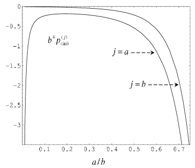
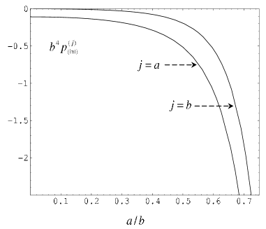
Figure 1: Vacuum interaction forces acting per unit surfaces of the cylindrical shells as functions of $a/b$. The left panel corresponds to the case of $D=3$ massless Dirichlet scalar and the right one is for Neumann scalar.

In figure 2 we present the same graphs for the Robin boundary conditions with the coefficients $B_{a}=0$, $B_{b}/(A_{b}b)=-0.2$. The left panel corresponds to the minimally coupled scalar and the right one is for a conformally coupled scalar. As we see, for the considered example the interaction force are repulsive for small distances between the surfaces and are attractive for large distances. This provides a possibility for the stabilization of the radii by the vacuum forces. However, it should be noted that to make reliable predictions regarding quantum stabilization, the renormalized single shell parts $p_{1}^{(j)}$ also should be taken into account.

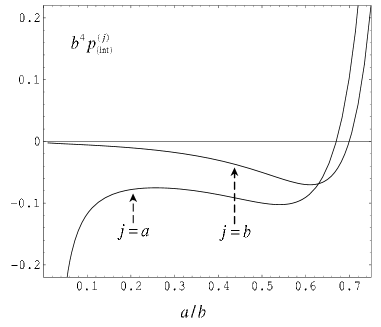
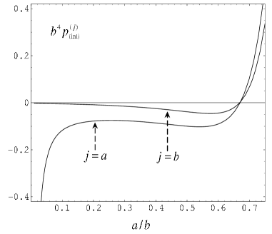
Figure 2: The same as in figure 1 for minimally (left panel) and conformally (right panel) coupled Robin scalars with $B_{a}=0$, $B_{b}/(A_{b}b)=-0.2$.

5 Casimir energy

In this section we consider the total vacuum energy for the configuration of two coaxial cylindrical boundaries. In the region between the boundaries the total vacuum energy per unit hypersurface in the axial direction is the sum of the zero-point energies of elementary oscillators:

$$E_{a\leqslant r\leqslant b}=\int\frac{d^{N}{\mathbf{k}}}{(2\pi)^{N}}\sideset{}{{}^{\prime}}{\sum}_{n=0}^{\infty}\sum_{l=1}^{\infty}(k^{2}+m^{2}+\sigma_{n,l}^{2}/a^{2})^{1/2}.$$ (53)

The expression on the right is divergent and to deal with this divergence we take the zeta function approach (for the application of the zeta function technique to the calculations of the Casimir energy see [42] and references therein). We consider the related zeta function

$$\zeta(s)=\mu^{s+1}\int\frac{d^{N}{\mathbf{k}}}{(2\pi)^{N}}\sideset{}{{}^{\prime}}{\sum}_{n=0}^{\infty}\sum_{l=1}^{\infty}(k^{2}+\sigma_{n,l}^{2}/a^{2}+m^{2})^{-s/2},$$ (54)

where the parameter $\mu$ with dimension of mass is introduced by dimensional reasons. Evaluating the integral over ${\mathbf{k}}$ we present this function in the form

$$\zeta(s)=\frac{\mu^{s+1}}{(4\pi)^{\frac{N}{2}}}\frac{\Gamma\left(\frac{s-N}{2}\right)}{\Gamma\left(\frac{s}{2}\right)a^{N-s}}\sideset{}{{}^{\prime}}{\sum}_{n=0}^{\infty}\zeta_{n}\left(s-N\right),$$ (55)

with the partial zeta function

$$\zeta_{n}\left(s\right)=\sum_{l=1}^{\infty}(\sigma_{n,l}^{2}+m^{2}a^{2})^{-s/2}.$$ (56)

We need to perform the analytic continuation of the sum on the right of (55) to the neighborhood of $s=-1$. An immediate consequence of the Cauchy’s formula for the residues of a complex function is the expression

$$\zeta_{n}\left(s\right)=\frac{1}{2\pi i}\int_{C}dz\,(z^{2}+m^{2}a^{2})^{-s/2}\frac{\partial}{\partial z}\ln C_{n}^{ab}(\eta,z),$$ (57)

where $C$ is a closed counterclockwise contour in the complex $z$ plane enclosing all zeros $\sigma_{n,l}$. We assume that this contour is made of a large semicircle (with radius tending to infinity) centered at the origin and placed to its right, plus a straight part overlapping the imaginary axis and avoiding the points $\pm iam$ by small semicircles in the left half-plane. When the radius of the large semicircle tends to infinity the corresponding contribution into $\zeta_{n}\left(s\right)$ vanishes for ${\mathrm{Re}}\,s>1$. Let us denote by $C^{1}$ and $C^{2}$ the upper and lower halves of the contour $C$. The integral on the right of Eq. (57) can be presented in the form

$$\zeta_{n}\left(s\right) = \frac{1}{2\pi i}\int_{C}dz\,(z^{2}+m^{2}a^{2})^{-s/2}\frac{\partial}{\partial z}\ln\left[z^{-n}\bar{J}_{n}^{(b)}(\eta z)\right]$$ (58)

$$+\frac{1}{2\pi i}\sum_{\alpha=1,2}\int_{C^{\alpha}}dz\,(z^{2}+m^{2}a^{2})^{-s/2}\frac{\partial}{\partial z}\ln\left[z^{n}\bar{H}_{n}^{(\alpha a)}(z)\right]$$

$$+\frac{1}{2\pi i}\sum_{\alpha=1,2}\int_{C^{\alpha}}dz\,(z^{2}+m^{2}a^{2})^{-s/2}\frac{\partial}{\partial z}\ln\left[1-\frac{\bar{J}_{n}^{(a)}(z)\bar{H}_{n}^{(\alpha b)}(\eta z)}{\bar{H}_{n}^{(\alpha a)}(z)\bar{J}_{n}^{(b)}(\eta z)}\right],$$

where $H_{n}^{(\alpha)}(z)$ are the Hankel functions. After parameterizing the integrals over imaginary axis we see that the parts of the integrals over $(0,\pm ima)$ cancel and we arrive at the expression

$$\zeta_{n}\left(s\right) = \frac{1}{\pi}\sin\frac{\pi s}{2}\int_{ma}^{\infty}dz\,(z^{2}-m^{2}a^{2})^{-s/2}\frac{\partial}{\partial z}\Bigg{\{}\ln\left[z^{-n}\bar{I}_{n}^{(b)}(\eta z)\right]$$ (59)

$$+\ln\left[z^{n}\bar{K}_{n}^{(a)}(z)\right]+\ln\left(1-\frac{\bar{I}_{n}^{(a)}(z)\bar{K}_{n}^{(b)}(\eta z)}{\bar{K}_{n}^{(a)}(z)\bar{I}_{n}^{(b)}(\eta z)}\right)\Bigg{\}}.$$

The integral with the last term in square brackets on the right of this formula is finite at $s=-(N+1)$ and vanishes in the limits $a\rightarrow 0$ or $b\rightarrow\infty$. The integrals with the first and second terms in the square brackets correspond to the partial zeta functions for the region inside a cylindrical shell with radius $b$ and for the region outside a cylindrical shell with radius $a$, respectively. As a result the total energy in the region $a\leqslant r\leqslant b$ is presented in the form

$$E_{a\leqslant r\leqslant b}=\zeta(s)|_{s=-1}=E_{r\geqslant a}^{(a)}+E_{r\leqslant b}^{(b)}+\Delta E,$$ (60)

where $E_{r\geqslant a}^{(a)}$ ($E_{r\leqslant b}^{(b)}$) is the vacuum energy for the region outside (inside) a cylindrical shell with radius $a$ ($b$) and the interference term is given by the formula

$$\Delta E = -\frac{(4\pi)^{\frac{1-D}{2}}}{\Gamma(\frac{D+1}{2})}\sideset{}{{}^{\prime}}{\sum}_{n=0}^{\infty}\int_{m}^{\infty}du\,(u^{2}-m^{2})^{\frac{D-1}{2}}\frac{\partial}{\partial u}\ln\left|1-\frac{\bar{I}_{n}^{(a)}(au)\bar{K}_{n}^{(b)}(bu)}{\bar{K}_{n}^{(a)}(au)\bar{I}_{n}^{(b)}(bu)}\right|$$ (61)

$$= \pi A_{D}\sideset{}{{}^{\prime}}{\sum}_{n=0}^{\infty}\int_{m}^{\infty}du\,u(u^{2}-m^{2})^{\frac{D-3}{2}}\ln\left|1-\frac{\bar{I}_{n}^{(a)}(au)\bar{K}_{n}^{(b)}(bu)}{\bar{K}_{n}^{(a)}(au)\bar{I}_{n}^{(b)}(bu)}\right|$$

To obtain the first of these formulae from the corresponding zeta function we have used the relation $\Gamma(x)\sin\pi x=\pi/\Gamma(1-x)$ for the gamma function. The interaction part of the vacuum energy (61) is negative for Dirichlet or Neumann boundary conditions and positive for Dirichlet boundary condition on one shell and Neumann boundary condition on the another. By the way similar to that used before for the case of the interaction forces it can be seen that in the limit $a,b\rightarrow\infty$ for fixed $b-a$ the corresponding result is obtained for parallel plates. In the limit $a\rightarrow 0$ for $A_{a},B_{a}\neq 0$ the main contribution into the interaction part of the vacuum energy comes from $n=0$ term. By using the expansions for the Bessel modified functions for small values of the argument to the leading order one finds

$$\Delta E\approx A_{D}\frac{\pi A_{a}a}{2B_{a}}\int_{m}^{\infty}du\,u(u^{2}-m^{2})^{\frac{D-3}{2}}\frac{\bar{K}_{0}^{(b)}(bu)}{\bar{I}_{0}^{(b)}(bu)}.$$ (62)

In the same limit and for Dirichlet boundary condition on the inner cylinder, $B_{a}=0$, the leading behavior for $\Delta E$ is obtained from (62) by the replacement $A_{a}a/B_{a}\rightarrow\ln(a/b)$. In the case of Neumann boundary condition on $r=a$, the main contribution comes from $n=0$ and $n=1$ terms and $\Delta E$ vanishes as $a^{2}$:

$$\Delta E\approx A_{D}\frac{\pi a^{2}}{2}\int_{m}^{\infty}du\,u^{3}(u^{2}-m^{2})^{\frac{D-3}{2}}\sideset{}{{}^{\prime}}{\sum}_{n=0}^{1}\frac{\bar{K}_{n}^{(b)}(bu)}{\bar{I}_{n}^{(b)}(bu)}$$

In the limit $b\rightarrow\infty$ and for a massless scalar field we have an asymptotic behavior with the leading term coming from $n=0$ summand:

$$\Delta E\approx\frac{\pi A_{D}}{2b^{D-1}\ln(a/b)}\int_{0}^{\infty}du\,u^{D-2}\frac{K_{0}(u)}{I_{0}(u)},$$ (63)

assuming that $A_{a},A_{b}\neq 0$. For $A_{a}=0$ and $A_{b}\neq 0$ the main contribution into the interaction part of the vacuum energy comes from $n=0$ and $n=1$ terms:

$$\Delta E\approx\frac{\pi a^{2}A_{D}}{2b^{D+1}}\int_{0}^{\infty}du\,u^{D}\sideset{}{{}^{\prime}}{\sum}_{n=0}^{1}\frac{K_{n}(bu)}{I_{n}(bu)}.$$ (64)

For the Neumann boundary condition on the outer cylinder, $A_{b}=0$, in the integrands of (63) and (64) instead of ratio of the Bessel modified functions the ratio of their derivatives stands. For a massive field and large values for the radius of the outer cylinder, under the condition $mb\gg 1$ the main contribution into the integral over $u$ in Eq. (61) comes from the lower limit of the integral. By using the asymptotic formulae for the Bessel modified function for large values of the argument, to the leading order we find

$$\Delta E\approx-\frac{2^{1-D}m^{\frac{D-1}{2}}}{\pi^{\frac{D-3}{2}}b^{\frac{D-1}{2}}}\frac{A_{b}-B_{b}m}{A_{b}+B_{b}m}e^{-2mb}\sideset{}{{}^{\prime}}{\sum}_{n=0}^{\infty}\frac{\bar{I}_{n}^{(a)}(am)}{\bar{K}_{n}^{(a)}(am)},$$ (65)

and the interaction part of the vacuum energy is exponentially suppressed. In figure 3 we have plotted the dependence of the interaction parts (full curves) in the total vacuum energy on the ratio $a/b$ for $D=3$ massless scalar fields with Dirichlet, Neumann and Robin boundary conditions. For the Robin case we have chosen the parameters in the boundary conditions as $B_{a}=0$, $B_{b}/(A_{b}b)=-0.2$.

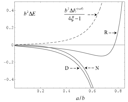
Figure 3: Interaction parts of the total and surface energies as functions of $a/b$. The graphs are plotted for $D=3$ massless scalar fields with Dirichlet (D) and Neumann (D) boundary conditions and in the case of Robin (R) boundary condition with $B_{a}=0$, $B_{b}/(A_{b}b)=-0.2$.

To obtain the total Casimir energy, $E$, we need to add to the energy in the region between the shells, given by Eq. (61), the energies coming from the regions $r\leqslant a$ and $r\geqslant b$. As a result one receives

$$E=\sum_{j=a,b}E^{(j)}+\Delta E,$$ (66)

where $E^{(j)}$ is the Casimir energy for a single cylindrical shell with the radius $j$. The latter is investigated in Ref. [22] as a function on the ratio of coefficients in Robin boundary condition. In particular, for Dirichlet and Neumann massless scalars one has the Casimir energies $E_{D}^{(j)}=6.15\cdot 10^{-4}j^{-2}$ and $E_{N}^{(j)}=-1.42\cdot 10^{-2}j^{-2}$ (see [12]). Note that in the total vacuum energy single boundary parts dominate for small values of the ratio $a/b$ and the interaction part is dominant for $a/b\lesssim 1$. In particular, combining the results for the single surface energies with the graphs from figure 3, we see that the total Casimir energy for a massless Dirichlet scalar in the geometry of two cylindrical shells is positive for small values $a/b$ and is negative for $a/b\lesssim 1$. For Neuamnn case the vacuum energy is negative for all values $a/b$ and has a maximum for some intermediate value of this ratio.

The total volume energy in the region $a\leqslant r\leqslant b$ is derived by the integration of ${{}_{0}^{0}}$-component of the volume energy-momentum tensor over this region:

$$E^{{\mathrm{(vol)}}}=2\pi\int_{a}^{b}dr\,r\langle 0|T_{0}^{0}|0\rangle.$$ (67)

Substituting mode-sum expansion (11) into formula (31), after the integration for the volume part of the vacuum energy we obtain

$$E^{{\mathrm{(vol)}}}=E_{a\leqslant r\leqslant b}-\pi(4\xi-1)\sum_{j=a,b}\frac{jA_{j}}{B_{j}}\langle 0|\varphi^{2}|0\rangle_{r=j}.$$ (68)

As we see this energy differs from the total Casimir energy (53) (see Ref. [36] for the discussion in general case of bulk and boundary geometries). This difference is due to the presence of the surface energy located on the bounding surfaces. By using the standard variational procedure, in Ref. [36] it has been shown that the energy-momentum tensor for a scalar field on manifolds with boundaries in addition to the bulk part contains a contribution located on the boundary. For an arbitrary smooth boundary $\partial M_{s}$ with the inward-pointing unit normal vector $n^{l}$, the surface part of the energy-momentum tensor is given by the formula

$$T_{ik}^{\mathrm{(surf)}}=\delta(x;\partial M_{s})\tau_{ik}$$ (69)

with

$$\tau_{ik}=\xi\varphi^{2}K_{ik}-(2\xi-1/2)h_{ik}\varphi n^{l}\nabla_{l}\varphi,$$ (70)

and the ’one-sided’ delta-function $\delta(x;\partial M_{s})$ locates this tensor on $\partial M_{s}$. In Eq. (70), $K_{ik}$ is the extrinsic curvature tensor of the boundary $\partial M_{s}$ and $h_{ik}$ is the corresponding induced metric. In the region between the cylindrical surfaces for separate boundaries one has $K_{ik}^{(j)}=-jn_{j}\delta_{i}^{2}\delta_{k}^{2}$, $j=a,b$. Now substituting the eigenfunctions into the corresponding mode-sum formula and using the boundary conditions, for the surface energy-momentum tensor on the boundary $r=j$ one finds

$$\langle 0|\tau_{i}^{(j)k}|0\rangle=\left[-\xi jn_{j}\delta_{i}^{2}\delta_{2}^{k}+(2\xi-1/2)\delta_{i}^{k}A_{j}/B_{j}\right]\langle 0|\varphi^{2}|0\rangle_{r=j},$$ (71)

for $i,k=0,1,\ldots,D$, and $\langle 0|\tau_{1}^{(j)1}|0\rangle=0$. From (71) for the surface energy we obtain the formula

$$E^{{\mathrm{(surf)}}}=2\pi\int_{a}^{b}dr\,r\langle 0|T_{0}^{\mathrm{(surf)}0}|0\rangle=\pi(4\xi-1)\sum_{j=a,b}\frac{jA_{j}}{B_{j}}\langle 0|\varphi^{2}|0\rangle_{r=j},$$ (72)

which, in accordance with (68), exactly coincides with the difference between the total and volume energies. Of course, the VEVs of the field square on the right of this formula and, hence, the surface energy-momentum tensor diverge and need some regularization with further renormalization. Note that due to the surface divergences the subtraction of the boundary-free part is not sufficient to obtain the finite result and additional renormalization procedure is needed. In particular, the generalized zeta function method is in general very powerful to give physical meaning to the divergent quantities. However, in this paper we will not go into the details of the renormalization for the surface energy-momentum tensor for a single cylindrical boundary. This investigation will be presented in the forthcoming paper [40]. Here we note that after the subtraction of the boundary-free part the remained divergences in the surface energy-momentum tensor are the same as those for a single surfaces when the second surface is absent. The additional parts induced by the presence of the second surface are finite and can be obtained by using the representation of the VEV for the field square given by formula (26). By taking into account the relation (43), the surface energy on the boundary $r=j$ is presented in the form

$$E_{j}^{{\mathrm{(surf)}}}=E_{1j}^{{\mathrm{(surf)}}}+\Delta E_{j}^{{\mathrm{(surf)}}},$$ (73)

where $E_{1j}^{{\mathrm{(surf)}}}$ is the surface energy for a single cylindrical boundary with radius $j$ when the second boundary is absent and the term

$$\Delta E_{j}^{{\mathrm{(surf)}}}=-\pi(4\xi-1)A_{D}\frac{A_{j}B_{j}}{j}\sideset{}{{}^{\prime}}{\sum}_{n=0}^{\infty}\int_{m}^{\infty}du\,u\left(u^{2}-m^{2}\right)^{\frac{D-3}{2}}\Omega_{jn}(au,bu)$$ (74)

is induced by the presence of the second boundary. The latter is finite for all non-zero intersurface distances. Note that on the base of relation (45) it can also be written in the form

$$\Delta E_{j}^{{\mathrm{(surf)}}} = -\pi A_{D}(4\xi-1)\sideset{}{{}^{\prime}}{\sum}_{n=0}^{\infty}\int_{m}^{\infty}du\,u\left(u^{2}-m^{2}\right)^{\frac{D-3}{2}}$$ (75)

$$\times\frac{n_{j}A_{j}B_{j}}{B_{jn}(u)}\frac{\partial}{\partial j}\ln\left|1-\frac{\bar{I}_{n}^{(a)}(au)\bar{K}_{n}^{(b)}(bu)}{\bar{I}_{n}^{(b)}(bu)\bar{K}_{n}^{(a)}(au)}\right|,$$

where $B_{jn}(u)$  is defined by Eq. (46). Now, by using formulae (40), (61), (75) it can be explicitly checked the relation

$$\Delta E=\Delta E^{\mathrm{(vol)}}+\sum_{j=a,b}\Delta E_{j}^{{\mathrm{(surf)}}}$$ (76)

for the interaction parts of the separate energies. In figure 3 we have plotted the interaction part of the surface energy (dashed curve) for the case of $D=3$ massless Robin scalar with $B_{a}=0$, $B_{b}/(A_{b}b)=-0.2$ as a function on the ratio $a/b$. For the considered example this energy is located on the surface $r=b-0$ of the outer cylinder. The surface energies for Dirichlet and Neumann scalars vanish.

Now let us explicitly check that for the interaction parts the standard energy balance equation is satisfied. We expect that in the presence of the surface energy this equation will be in the form

$$dE=-pdV+\sum_{j=a,b}\frac{E_{j}^{{\mathrm{(surf)}}}}{2\pi j}dS^{(j)},$$ (77)

where $V=\pi(b^{2}-a^{2})$ and $S^{(j)}=2\pi j$ are the volume and surface area per unit hypersurface in the axial direction. In Eq. (77), $p$ is the perpendicular vacuum stress on the boundary and is determined by the vacuum expectation value of the ${}_{1}^{1}$-component of the bulk energy-momentum tensor: $p=-\langle 0|T_{1}^{1}|0\rangle$. From equation (77) one obtains

$$\frac{\partial E}{\partial j}=2\pi jn_{j}p^{(j)}+E_{j}^{{\mathrm{(surf)}}}/j,$$ (78)

with $p^{(j)}$ being the perpendicular vacuum stress on the boundary $r=j$. Assuming that relation (78) is satisfied for the single boundary parts, for the interference parts we find

$$\frac{\partial\Delta E}{\partial j}=2\pi jn_{j}p_{{\mathrm{(int)}}}^{(j)}+\Delta E_{j}^{{\mathrm{(surf)}}}/j.$$ (79)

Now by taking into account expressions (47), (61), (75) for the separate terms in this formula and integrating by part in (61), we see that this relation indeed takes place. Hence, we have explicitly checked that the vacuum energies and effective pressures on the boundaries obey the standard energy balance equation. Note that here the role of the surface energy is crucial and the vacuum forces acting on the boundary evaluated from the bulk stress tensor [determined by $p_{{\mathrm{(int)}}}^{(j)}$], in general, can not be obtained by a simple differentiation of the total vacuum energy. The second term on the right of formula (79) corresponds to the additional pressure acting on the curved boundary. Noting that $\Delta E_{j}^{{\mathrm{(surf)}}}/(2\pi j)$ is the corresponding surface energy density, we see that this pressure is determined by Laplace formula. The total pressure on the boundary evaluated as the sum of bulk and surface parts is related to the total vacuum energy by standard formula and does not depend on the curvature coupling parameter.

6 Conclusion

In the present paper, we have investigated the one-loop quantum vacuum effects produced by two coaxial cylindrical shells in the $(D+1)$-dimensional Minkowski spacetime. The case of a massive scalar field with general curvature coupling parameter and satisfying the Robin boundary conditions on the boundaries is considered. To derive formulae for the VEVs of the field operator squared and the energy-momentum tensor, we first construct the positive frequency Wightman function. This function is also important in considerations of the response of a particle detector at a given state of motion through the vacuum under consideration [38]. The application of a variant of the generalized Abel-Plana formula to the mode-sum over zeros of the combinations of the cylindrical functions allowed us to extract the parts due to a single cylindrical boundary and to present the second boundary induced parts in terms of the exponentially convergent integrals. For the exterior and interior regions of a single cylindrical shell the Wightman functions are given by formulae (20) and (24) respectively. The second boundary induced parts are presented by the last terms on the right of formulae (19) and (23). The VEVs of the field square and the energy-momentum tensor are obtained by the evaluation of the Wightman function and the combinations of its derivatives in the coincidence limit of arguments. In both cases the expectation values are presented as the sum of single boundary induced and interference terms. The surface divergences in the VEVs of the local observables are contained in the single boundary parts and the interference parts are finite on both boundaries. In particular, the integrals in the corresponding formulae are exponentially convergent and they are useful for numerical evaluations. Due to the presence of boundaries the vacuum stresses in radial, azimuthal and axial directions are anisotropic. For the axial stress and the energy density we have standard relation for the unbounded vacuum. We have considered various limiting cases of the formulae for the interference parts. In particular, in the limit $a,b\rightarrow\infty$ for a fixed value $b-a$, we recover the result for the geometry of two parallel Robin plates on the Minkowski background. The vacuum forces acting on boundaries are considered in section 4. These forces contain two terms. The first ones are the forces acting on a single surface then the second boundary is absent. Due to the well-known surface divergences in the VEVs of the energy-momentum tensor these forces are infinite and need an additional regularization with further renormalization. The another terms in the vacuum forces are finite and are induced by the presence of the second boundary. They correspond to the interaction forces between the boundaries and are determined by formula (44) or equivalently by formula (47). For the Dirichlet and Neumann scalars these forces are always attractive and they are repulsive for the mixed Dirichlet-Neumann case. In the case of general Robin scalar the interaction forces can be both attractive or repulsive in dependence of the coefficients in the boundary conditions and the distance between the boundaries. As an illustration, in figure 2 we present an example when the interaction forces are repulsive for small distances and are attractive for large distances. This provides a possibility for the stabilization of the radii by vacuum forces. However, it should be noted that for the reliable predictions regarding quantum stabilization, the renormalized single shell parts also should be taken into account. In section 5 we consider the total vacuum energy in the region between the cylindrical surfaces, evaluated as the sum of the zero-point energies for elementary oscillators. It is argued that this energy differs from the energy, obtained by the integration of the volume energy density over the region between the boundaries. We show that this difference is due to the presence of the surface energy located on the bounding surfaces. Further for the evaluation of the total and surface energies we use the zeta function technique. They are presented as the sum of single boundary and interaction parts. The latter are given by formula (61) for the total vacuum energy and by formula (75) for the surface energy and are finite for all nonzero values of the intersurface separation. In the total vacuum energy single boundary parts dominate for small values of the ratio $a/b$ and the interaction part is dominant for $a/b\lesssim 1$. For an arbitrary number of spatial dimensions and independent on the value of the mass, the interaction part of the vacuum energy is negative for Dirichlet or Neumann boundary conditions and is positive for Dirichlet boundary condition on one shell and Neumann boundary condition on the another. Further, we have shown that the induced vacuum densities and vacuum effective pressures on the cylindrical surfaces satisfy the energy balance equation (77) with the inclusion of the surface terms, which can also be written in the form (79).

References

- [1] H.B.G. Casimir, Proc. Kon. Ned. Akad. Wetensch. B 51, 793 (1948).
- [2] V.M. Mostepanenko and N.N. Trunov, The Casimir Effect and Its Applications (Oxford University Press, Oxford, 1997).
- [3] G. Plunien, B. Muller and W. Greiner, Phys. Rep. 134, 87 (1986).
- [4] M. Bordag, U. Mohidden, and V.M. Mostepanenko, Phys. Rep. 353, 1 (2001).
- [5] K.A. Milton, The Casimir Effect: Physical Manifestation of Zero–Point Energy (World Scientific, Singapore, 2002).
- [6] M. Bordag and K. Kirsten, Phys. Rev. D 53, 5753 (1996); M. Bordag and K. Kirsten, Phys. Rev. D 60, 105019 (1999); M. Schaden and L. Spruch, Phys. Rev. A 58, 935 (1998); M. Schaden and L. Spruch, Phys. Rev. Lett. 84, 459 (2000); R. Golestanian and M. Kardar, Phys. Rev. A 58, 1713 (1998); T. Emig and R. Buscher, Nucl. Phys. B 696, 468 (2004); N. Graham, R.L. Jaffe, V. Khemani, M. Quandt, M. Scandurra, and H. Weigel, Nucl. Phys. B 645, 49, (2002); N. Graham, R.L. Jaffe, and H. Weigel, Int. J. Mod. Phys. A 17, 846 (2002); N. Graham, R.L. Jaffe, V. Khemani, M. Quandt, M. Scandurra, and H. Weigel, Phys. Lett. B572, 196 (2003); H. Gies, K. Langfeld, and L. Moyaerts, JHEP 0306, 018 (2003); A. Scardicchio and R.L. Jaffe, Phys. Rev. Lett. 92, 070402 (2004); A. Scardicchio and R.L. Jaffe, Nucl. Phys. B 704, 552, (2005); A. Bulgac, P. Magierski, and A. Wirzba, hep-th/0511056.
- [7] P. Fishbane, S. Gasiorowicz and P. Kaus, Phys. Rev. D 36, 251 (1987); P. Fishbane, S. Gasiorowicz and P. Kaus, Phys. Rev. D 37, 2623 (1988).
- [8] B.M. Barbashov and V.V. Nesterenko, Introduction to the Relativistic String Theory (World Scientific, Singapore, 1990).
- [9] J. Ambjørn and S. Wolfram, Ann. Phys. 147, 1 (1983).
- [10] L.L. De Raad Jr. and K.A. Milton, Ann. Phys. 136, 229 (1981).
- [11] K.A. Milton, A.V. Nesterenko and V.V. Nesterenko, Phys. Rev. D 59, 105009 (1999).
- [12] P. Gosdzinsky and A. Romeo, Phys. Lett. B 441, 265 (1998).
- [13] G. Lambiase, V.V. Nesterenko, and M. Bordag, J. Math. Phys. 40, 6254 (1999).
- [14] A.A. Saharian, Izv. AN Arm. SSR. Fizika 23, 130 (1988) [Sov. J. Contemp. Phys. 23, 14 (1988)].
- [15] A.A. Saharian, Dokladi AN Arm. SSR 86, 112 (1988) (Reports NAS RA, in Russian).
- [16] A.A. Saharian, The generalized Abel-Plana formula. Applications to Bessel functions and Casimir effect. Preprint IC/2000/14, hep-th/0002239.
- [17] F.D. Mazzitelli, M.J. Sanchez, N.N. Scoccola, J. von Stecher, Phys. Rev. A 67, 013807 (2002); D.A.R. Dalvit, F.C. Lombardo, F.D. Mazzitelli, R. Onofrio, Europhys. Lett. 67, 517 (2004); F.D. Mazzitelli, in Quantum Field Theory under the Influence of External Conditions, ed. by K. A. Milton (Rinton Press, Princeton NJ, 2004), quant-ph/0406116.
- [18] V.V. Nesterenko, G. Lambiase, and G. Scarpetta, J. Math. Phys. 42, 1974 (2001).
- [19] A.H. Rezaeian and A.A. Saharian, Class. Quantum Grav. 19, 3625 (2002); A.A. Saharian and A.S. Tarloayn, J. Phys. A 38, 8763 (2005).
- [20] I. Brevik and G.H. Nyland, Ann. Phys. 230, 321 (1994); V.V. Nesterenko and I.G. Pirozhenko, Phys. Rev. D 60, 125007 (1999); I. Klich and A. Romeo, Phys. Lett. B 476, 369 (2000); G. Barton, J. Phys. A 34, 4083 (2001); I. Cavero-Peláez and K.A. Milton, Ann. Phys. 320, 108 (2005); A. Romeo and K.A. Milton, Phys. Lett. B 621, 309 (2005); I. Brevik and A. Romeo, hep-th/0601211.
- [21] A.A. Saharian and A.S. Kotanjyan, Nucl. Instrum. Meth. B 226, 351 (2004); A.A. Saharian and A.S. Kotanjyan, J. Phys. A 38, 4275 (2005).
- [22] A. Romeo and A.A. Saharian, Phys. Rev. D 63, 105019 (2001).
- [23] V.M. Mostepanenko and N.N. Trunov, Sov. J. Nucl. Phys. 42, 812 (1985).
- [24] S.L. Lebedev, Yadernaya Fizika 64, 1413 (2001) (Physics of Atomic Nuclei 64, 1337 (2001)).
- [25] S.N. Solodukhin, Phys. Rev. D 63, 044002 (2001).
- [26] J. Ambjørn and S. Wolfram, Ann. Phys. 147, 33 (1983).
- [27] I.G. Moss, Class. Quantum Grav. 6, 759 (1989).
- [28] G. Esposito and A.Yu. Kamenshchik, Class. Quantum Grav. 12, 2715 (1995).
- [29] G. Esposito, A.Yu. Kamenshchik, and G. Polifrone, Euclidean Quantum Gravity on Manifolds with Boundary (Kluwer, Dordrecht, 1997).
- [30] T. Gherghetta and A. Pomarol, Nucl. Phys. B 586, 141 (2000); A. Flachi and D.J. Toms, Nucl. Phys. B 610, 144 (2001); A.A. Saharian, Nucl. Phys. B 712, 196 (2005).
- [31] A. Romeo and A.A. Saharian, J. Phys. A 35, 1297 (2002).
- [32] G. Kennedy, R. Critchley, and J.S. Dowker, Ann. Phys. 125, 346 (1980).
- [33] S.A. Fulling, J. Phys. A 36, 6857 (2003).
- [34] A.A. Saharian, Phys. Rev. D 63, 125007 (2001).
- [35] I. Cavero-Peláez, K.A. Milton, and J. Wagner, hep-th/0508001.
- [36] A.A. Saharian, Phys. Rev. D 69, 085005 (2004).
- [37] A.A. Saharian, Phys. Rev. D 70, 064026 (2004).
- [38] N. D. Birrell and P. C. W. Davies, Quantum Fields in Curved Space (Cambridge University Press, Cambridge, 1982).
- [39] A.P. Prudnikov, Yu.A. Brychkov, and O.I. Marichev, Integrals and Series (Gordon and Breach, New York, 1986), Vol.2.
- [40] A.A. Saharian and A.S. Tarloyan, in preparation.
- [41] M. Abramowitz and I.A. Stegun, Handbook of Mathematical functions (National Bureau of Standards, Washington DC, 1964).
- [42] E. Elizalde, S.D. Odintsov, A. Romeo, A.A. Bytsenko, and S. Zerbini, Zeta Regularization Techniques with Applications (World Scientific, Singapore, 1994); K. Kirsten, Spectral Functions in Mathematics and Physics (Chapman and Hall/CRC, Boca Raton, 2002).