Stringy Black Holes and the Geometry of Entanglement

Abstract

Recently striking multiple relations have been found between pure state $2$ and $3$-qubit entanglement and extremal black holes in string theory. Here we add further mathematical similarities which can be both useful in string and quantum information theory. In particular we show that finding the frozen values of the moduli in the calculation of the macroscopic black hole entropy in the STU model, is related to finding the canonical form for a pure three qubit entangled state defined by the dyonic charges. In this picture the extremization of the BPS mass with respect to moduli is connected to the problem of finding the optimal local distillation protocol of a GHZ state from an arbitrary three-qubit pure state. These results and a geometric classification of STU black holes BPS and non-BPS can be described in the elegant language of twistors. Finally an interesting connection between the black hole entropy and the average real entanglement of formation is established.

I Introduction

Recently there has been much progress in seemingly two unrelated fields of theoretical physics. One of them is quantum information theory which concerns the study of quantum entanglement the ”characteristic trait of quantum mechanics”Sch and its possible applications such as quantum teleportation Bennett , quantum cryptography Ben2 and more importantly quantum computing Nielsen . The other is the physics of stringy black holes which has provided spectacular results such as the black hole attractor mechanismFerrara and the microscopic calculation of the black hole entropyStrominger related to the nonperturbative symmetries found between different string theories Hull ; Witten ; Polchinski .

As far as mathematics is concerned these two different strains of knowledge have turned out to be related when DuffDuff pointed out that the entropy of the so called extremal BPS STU black hole can be expressed in a very compact way in terms of Cayley’s hyperdeterminantGelfand which plays a prominent role as the three-tangleckw in studies of three-qubit entanglement. Recently further mathematical similarities have been found by Kallosh and LindeLinde . They have shown that the entropy of the axion-dilaton black hole is related to the concurrence which is the unique pure two-qubit entanglement measure. They have streched the validity of the relationship between the three-tangle and the STU black hole entropy found by Duff to non-BPS black holes. They have also related the well-known entanglement classes of pure three-qubit entanglement to different classes of black holes in string theory. Finally they emphasized the univeral role of the Cartan-Cremmer-Julia $E_{7(7)}$ invariant playing as the expression for the entropy of black holes and black rings in $N=8$ supergravity/M-theory. By making use of the $SU(8)$ symmetry they have pointed out that the three-tangle shows up in this invariant too.

These results are intriguing mathematical connections arising from the similar symmetry properties of qubit systems and the web of dualities in the STU model. As far as classical supergravity is concerned the symmetry of the extremal STU model is $SL(2,{\bf R})^{\otimes 3}$, or taking into account quantum corrections and the quantized nature of electric and magnetic charges $SL(2,{\bf Z})^{\otimes 3}$. In string theory the latter symmetry group is also dictated by internal consistency. In qubit systems on the other hand the symmetry group in question is the group of stochastic local operations and classical communication (SLOCC) which is $SL(2,{\bf C})^{\otimes 3}$. Hence the groups connected to dualities occurring in stringy black holes are related to integers or at most to the real number system. However, the power of entanglement is related to the special role played by complex numbers in quantum theory. This manifests itself at the level of three-partite protocols in the use of the larger group $SL(2,{\bf C})^{\otimes 3}$ (or more generally in $GL(2,{\bf C})^{\otimes 3}$), giving rise to interesting complex geometryLevay1 similar to the one found in twistor theoryPenrose ; Ward .

In the treatments of Refs.Duff ; Linde instead of the $8$ complex numbers characterizing a general (unnormalized) three-qubit state the $8$ integers corresponding to the quantized electric and magnetic charges of $N=2$ , $D=4$ supergravity has been used. Hence in this case we have a correspondence between quantized charges and the integer amplitudes of a special class of (unnormalized) real three-qubit states. Already using these real quantum bits or rebitsCaves enabled the authors of Refs.Duff ; Linde to obtain amazing formal correspondences between stringy black holes and quantum entanglement. Now the question arises: can we find further relationships displaying the power of three-qubit entanglement in the more general complex context? One of the aims of the present paper is to answer this question in the affirmative. We show that the well-known process of finding the frozen values of the moduli for the calculation of the macroscopic black hole entropy in the STU model, is related to the problem of obtaining the canonical decomposition for the three-qubit states defined by the charges using complex SLOCC transformations. We also regard this paper as an attempt to establish some sort of dictionary between the languages used by string theorists and researchers working in the field of quantum information theory. In particular we would like to show how the general theory of complex three-qubit entanglement contains in the form of real states the important cases studied by string theorists in the special case of STU black holes.

The organization of the paper is as follows. In Section II. the background concerning three-qubit entanglement is presented. Here we also discuss the canonical form of three-qubit states (the analogue of the Schmidt decomposition for two-qubits), and its relationship to three-qubit invariants. Special attention is paid to the important special case of real states which will play the dominant role in subsequent chapters as the ones describing STU black holes. Here a new result concerning a geometric characterization of such real states embedded in the more general complex ones is obtained. In section III. in the context of the supersymmetric STU-model we present the quantum entanglement version of the well-known process of freezing the moduli by extremization of the BPS massFerrara . It turns out that this extremization is related to finding the optimal distillation protocol of a GHZ state in the entanglement picture. The solution of the stabilization equations resulting in the STU black hole entropy formula have been obtained in Shmakova . We show that the process of finding the frozen values of the moduli is just the one of obtaining a canonical form for the corresponding three-qubit state by employing complex SLOCC transformations. In Section IV. using the complex principal null directions of the two-plane in ${\bf C}^{4}$ containing the two real four-vectors of the charges we shed some light on the geometric meaning of this canonical form. Here an alternative geometric picture for the classification of BPS and non-BPS black holes small and large is also suggested. It is based on the intersection properties of a complex line in ${\bf CP}^{3}$ with a fixed quadric. Finally an interesting connection between the black hole entropy and the real entanglement of formation is established. This section also contains some comments and the conclusions.

II Three-qubit entanglement

An arbitrary (unnormalized) three-qubit pure state $|\psi\rangle\in{\bf C}^{2}\otimes{\bf C}^{2}\otimes{\bf C}^{2}$ is characterized by $8$ complex numbers ${\psi}_{lkj}$ with $l,k,j=0,1$ and can be written in the following form

$$|\psi\rangle=\sum_{l,k,j}{\psi}_{lkj}|lkj\rangle\quad|lkj\rangle\equiv{|l\rangle}_{C}\otimes{|k\rangle}_{B}\otimes{|j\rangle}_{A}.$$ (1)

We can imagine three parties (Alice, Bob and Charlie), wildly separated, possessing a qubit from the entangled three-qubit state $|\psi\rangle$. (Above we have adopted the convention of Ref. [13] of labelling these qubits from the right to the left.) In a class of quantum information protocols the parties can manipulate their qubits reversibly with some probability of success by performing local manipulations assisted by classical communication between them. Such protocols are yielding special transformations of the states, called stochastic local operations and classical communication (SLOCC). It can be shownVidal that such operations can be represented mathematically by applying the group $GL(2,{\bf C})^{\otimes 3}$ on the state $|\psi\rangle$ in the form

$$|\psi\rangle\mapsto({\cal C}\otimes{\cal B}\otimes{\cal A})|\psi\rangle,\quad{\cal C}\otimes{\cal B}\otimes{\cal A}\in GL(2,{\bf C})^{\otimes 3}.$$ (2)

Since we are interested in states up to a physically irrelevant complex constant we can fix the determinants of the $GL(2,{\bf C})$ transformations to one, hence we can assume that the group of SLOCC transformations is just $SL(2,{\bf C})^{\otimes 3}$.

In the SLOCC classification of pure three-qubit states one forms the space of equivalence classes ${\bf C}^{2}\otimes{\bf C}^{2}\otimes{\bf C}^{2}/SL(2,{\bf C})^{\otimes 3}$. The result is as followsVidal . We have six different equivalence classes. Four of them correspond to the completely separable class $(A)(B)(C)$ represented e.g. by $|000\rangle$, and three classes of biseparable states of the form $A(BC)$, $B(AC)$ and $C(AB)$ represented e.g. by $(|00\rangle+|11\rangle)\otimes|0\rangle$ for the first of them. The remaining two classes are the so-called Werner and Greenberger-Horne-Zeilinger classes represented by the states $|W\rangle=|001\rangle+|010\rangle+|100\rangle$ and $|GHZ\rangle=|000\rangle+|111\rangle$. Hence apart from the separable cases three qubits can be entangled in two essentially different ways. The class carrying the genuine tripartite entanglement is the GHZ class. It is known that the GHZ state appears as the maximally entangled stateGisin , it violates Bell-inequalities maximally and it maximizes the mutual information of local measurements, moreover it is the only state from which an EPR state can be obtained with certainty. On the other hand the W-state maximizes only two-qubit quantum correlationsVidal inside our three-qubit state.

There are a number of polynomial invariants characterizing these entanglement classes. The most important one is the $SL(2,{\bf C})^{\otimes 3}$ and permutation (triality) invariant three-tangleckw ${\tau}_{ABC}\equiv 4|D({\psi})|$ where

$$D({\psi}) \equiv {\psi}_{000}^{2}{\psi}_{111}^{2}+{\psi}_{001}^{2}{\psi}_{110}^{2}+{\psi}_{010}^{2}{\psi}_{101}^{2}+{\psi}_{011}^{2}{\psi}_{100}^{2}$$ (3)

$$- 2({\psi}_{000}{\psi}_{001}{\psi}_{110}{\psi}_{111}+{\psi}_{000}{\psi}_{010}{\psi}_{101}{\psi}_{111}$$

$$+ {\psi}_{000}{\psi}_{011}{\psi}_{100}{\psi}_{111}+{\psi}_{001}{\psi}_{010}{\psi}_{101}{\psi}_{110}$$

$$+ {\psi}_{001}{\psi}_{011}{\psi}_{110}{\psi}_{100}+{\psi}_{010}{\psi}_{011}{\psi}_{101}{\psi}_{100})$$

$$4 ({\psi}_{000}{\psi}_{011}{\psi}_{101}{\psi}_{110}+{\psi}_{001}{\psi}_{010}{\psi}_{100}{\psi}_{111})$$

is the Cayley hyperdeterminantGelfand . By chosing the first, second or third qubit one can introduce three sets of complex four vectors, e.g. by chosing the first i.e. Alice’s qubit we define

$${\xi}^{(A)}_{I}=\begin{pmatrix}{\psi}_{000}\\ {\psi}_{010}\\ {\psi}_{100}\\ {\psi}_{110}\end{pmatrix},\quad{\eta}^{(A)}_{J}=\begin{pmatrix}{\psi}_{001}\\ {\psi}_{011}\\ {\psi}_{101}\\ {\psi}_{111}\end{pmatrix}\quad I,J=1,\dots 4$$ (4)

similarly we can define the pairs of four-vectors $({\xi}^{(B)},{\eta}^{(B)})$ and $({\xi}^{(C)},{\eta}^{(C)})$. Alternatively one can define three bivectors $P^{(A)}={\xi}^{(A)}\wedge{\eta}^{(A)}$ with components (Plücker coordinates)

$$P^{(A)}_{IJ}={\xi}^{(A)}_{I}{\eta}^{(A)}_{J}-{\xi}^{(A)}_{J}{\eta}^{(A)}_{I}$$ (5)

and similarly with the label $A$ replaced by $B$ or $C$. Then we haveLevay1 ; Levay2

$${\tau}_{ABC}=2|P^{(A)}_{IJ}P^{(A)IJ}|=2|P^{(B)}_{IJ}P^{(B)IJ}|=2|P^{(C)}_{IJ}P^{(C)IJ}|,$$ (6)

where indices are raised with respect to the $SL(2,{\bf C})\times SL(2,{\bf C})$ invariant metric $g={\varepsilon}\otimes{\varepsilon}$

$$g^{IJ}=\begin{pmatrix}0&0&0&1\\ 0&0&-1&0\\ 0&-1&0&0\\ 1&0&0&0\end{pmatrix}=\begin{pmatrix}0&1\\ -1&0\end{pmatrix}\otimes\begin{pmatrix}0&1\\ -1&0\end{pmatrix}.$$ (7)

Since the Plücker coordinates (5) are $SL(2,{\bf C})$ invariant Eq. (6) shows the $SL(2,{\bf C})^{\otimes 3}$ invariance and triality at the same time. Notice that the three-tangle can also be written in the form

$${\tau}_{ABC}=4|({\xi}\cdot{\xi})({\eta}\cdot{\eta})-({\xi}\cdot{\eta})^{2}|=4|-D(\psi)|,$$ (8)

with ${\xi}\cdot{\eta}\equiv g^{IJ}{\xi}_{I}{\eta}_{J}$ and the possible labels $A,B,C$ of ${\xi}$ and ${\eta}$ are now supressed.

The physical importance of the three-tangle ${\tau}_{ABC}$ is that it discriminates between the two different types of three-qubit entanglement. For the W-class we have ${\tau}_{ABC}=0$ and for the GHZ-class ${\tau}_{ABC}\neq 0$. In order to also discriminate between different types of separability we need further invariants. These are defined as follows.

Let us define the one and two partite reduced density matrices

$${\rho}_{A}={\rm Tr}_{BC}|\psi\rangle\langle\psi|,\quad{\rho}_{BC}={\rm Tr}_{A}|\psi\rangle\langle\psi|,$$ (9)

and the quantities ${\rho}_{B},{\rho}_{C},{\rho}_{AC}$ and ${\rho}_{AB}$ are defined accordingly. Note, that the trace of these quantities for unnormalized pure three-qubit states is not fixed to one. Then we can define the quantity ${\tau}_{A(BC)}$ called the squared-concurrence between the subsystems $A$ and $BC$ as

$${\tau}_{A(BC)}=4{\rm Det}{\rho}_{A}=2\sum_{I,J=1}^{4}{\overline{P}}^{(A)}_{IJ}P^{(A)}_{IJ}.$$ (10)

Similarly one can define ${\tau}_{B(AC)}$ and ${\tau}_{C(AB)}$, using $P^{(B)}$ and $P^{(C)}$ respectively. Notice that now we have complex conjugation in the first factor and now the indices are not contracted by the metric $g$. In order to understand this by supressing subsystem labels we can alternatively write

$${\tau}_{A(BC)}=4(\langle{\xi}|{\xi}\rangle\langle{\eta}|{\eta}\rangle-{|\langle{\xi}|{\eta}\rangle|}^{2}),$$ (11)

where $\langle{\xi}|{\eta}\rangle=\sum_{\mu=1}^{4}\overline{\xi}_{I}{\eta}_{I}$. Eq. (11) should be compared with Eq.(8). We remark that the expressions for ${\tau}_{ABC}$ and ${\tau}_{A(BC)}$ can be written in a unified way by going to the ”magic base”Wootters via using a suitable unitary transformation. In this caseLevay1 ${\tau}_{ABC}=2|P_{MN}P^{MN}|$ and ${\tau}_{A(BC)}=2\overline{P}_{MN}P^{MN}$ where in this base indices are simply raised by ${\delta}^{MN}$ $M,N=1,2,3,4$ with $M$ and $N$ now labelling the components in the ”magic base”. This way of writing uses the fact that $(SL(2,{\bf C})\otimes SL(2,{\bf C}))/{\bf Z}_{2}\simeq O(4,{\bf C})$. Here, in order to establish connections with the formalism of stringy black holes, however, we follow a different route and use the somewhat more complicated expressions of Eqs. (6), and (10). Notice also the factors of $2$ appearing in these formulae. These are necessary for normalized states, since in this case all four quantities take values in the interval $[0,1]$.

Looking at Eq. (11) it is clear that ${\tau}_{A(BC)}=0$ if and only if ${\xi}^{(A)}$ and ${\eta}^{(A)}$ are linearly dependent. (We exclude the trivial cases with $\xi$ or $\eta$ vanishing.) This means that the corresponding reduced density matrix ${\rho}_{A}$ has rank one a condition equivalent to $A(BC)$ separability. Hence ${\tau}_{A(BC)}=0$ iff $|\psi\rangle$ is $A(BC)$ separable. Similarly the vanishing of the squared concurrences ${\tau}_{B(AC)}$ and ${\tau}_{C(AB)}$ indicate separability of the form $B(AC)$ and $C(AB)$.

What about the invariance properties of our quantities ${\tau}_{A(BC)}$ ,${\tau}_{B(AC)}$ and ${\tau}_{C(AB)}$? Clearly these quantities are individually invariant with respect to $SL(2,{\bf C})\otimes U(4)$, where the $SL(2,{\bf C})$ part is acting on the qubit which can be separated from the rest. However, all three quantities are left invariant merely with respect to the action of the subgroup $SU(2)^{\otimes 3}$.

Using the four invariants ${\tau}_{ABC}$, ${\tau}_{A(BC)}$, ${\tau}_{B(AC)}$ and ${\tau}_{C(AB)}$ one can obtain the classification of pure three-qubit statesVidal . For the completely separable class all of our invariants are vanishing. For the $A(BC)$ class only ${\tau}_{ABC}$ and ${\tau}_{A(BC)}$ is vanishing. After the appropriate permutations the same can be said for the remaining biseparable classes. For the W-class only ${\tau}_{ABC}$ is vanishing, and at last for the GHZ-class none of the invariants is vanishing.

How can we characterize two-partite correlations inside our three-qubit state? In order to do this we have to look at the density matrices ${\rho}_{AB}$, ${\rho}_{AC}$ and ${\rho}_{BC}$. Generally these states are mixed, so we have to characterize also two-qubit mixed-state entanglement. A useful measure for the most general type of two-qubit mixed-state entanglement isWootters ${\tau}_{AB}$ which is the squared-concurrence for the mixed state in question

$${\tau}_{AB}=\left({\rm max}\{{\lambda}_{1}-{\lambda}_{2}-{\lambda}_{3}-{\lambda}_{4},0\}\right)^{2}$$ (12)

where ${\lambda}_{i},i=1,2,3,4$ is the nonincreasing sequence of the square-roots of the eigenvalues of the nonnegative matrix

$${\rho}\tilde{\rho}\equiv{\rho}({\varepsilon}\otimes{\varepsilon})\overline{\rho}({\varepsilon}\otimes{\varepsilon}).$$ (13)

The quantities ${\tau}_{AC}$ and ${\tau}_{BC}$ are defined accordingly. Notice that the trace of the matrix ${\rho}\tilde{\rho}$ due to the Hermiticity of ${\rho}$ is an $SL(2,{\bf C})\times SL(2,{\bf C})$ invariant, since it is of the form

$${\rm Tr}({\rho}\tilde{\rho})={\rho}_{IJ}{\rho}^{IJ}.$$ (14)

Consequently the traces of all powers of the matrix ${\rho}\tilde{\rho}$ are also invariant with respect to this group. The result is that the quantities ${\tau}_{AB}$, ${\tau}_{BC}$ and ${\tau}_{AC}$ are $SL(2,{\bf C})\otimes SL(2,{\bf C})$ invariant too.

In the special case when the mixed two-qubit state sits inside the pure three-qubit state we have e.g.

$$({\rho}_{BC})_{IJ}={\xi}^{(A)}_{I}\overline{\xi}^{(A)}_{J}+{\eta}^{(A)}_{I}\overline{\eta}^{(A)}_{J},$$ (15)

i.e. all of our two-qubit mixed state density matrices have rank at most two. This means that in the formula (12) we have at most two nonzero eigenvalues ${\lambda}_{1}$ and ${\lambda}_{2}$. The invariants discussed above are not independent, they are subject to the important relationsckw

$${\tau}_{A(BC)}={\tau}_{AB}+{\tau}_{AC}+{\tau}_{ABC}$$ (16)

with the two other ones can be obtained by cyclic permutations. These relations implying that e.g. ${\tau}_{A(BC)}\leq{\tau}_{AB}+{\tau}_{AC}$ that are also called the entanglement monogamy relations expressing the fact that unlike classical, quantum correlations cannot be shared freely between the parties.

There is one more invariant whose geometric meaning was clarified in Ref.Levay1 . Consider a pure three-qubit state which is nonseparable (i.e. none of the quantities ${\tau}_{A(BC)}$, ${\tau}_{B(AC)}$ and ${\tau}_{C(AB)}$ is vanishing.) Then the three separable bivectors $P={\xi}\wedge{\eta}$ (in the following the labels $A$, $B$ and $C$ are implicit, we refer to the triple of these objects by using plural for the corresponding quantities) are giving rise to the planes $a{\xi}_{I}+b{\eta}_{I}$ with $a,b\in{\bf C}$. Then we can find the principal null directions of these planes by solving the quadratic equations $a^{2}({\xi}\cdot{\xi})+2ab({\xi}\cdot{\eta})+b^{2}({\eta}\cdot{\eta})=0$. The discriminant of these equations is just the Cayley hyperdeterminant so we have two principal null directions for ${\tau}_{ABC}\neq 0$ and one for ${\tau}_{ABC}=0$ for each plane. Hence the number of principal null directions corresponds to the two nonseparable three-qubit entanglement classes the W and the GHZ class. Assuming ${\xi}\cdot{\xi}\neq 0$ and solving the quadratic equations for the ratio $\frac{a}{b}$, these directions are

$$u_{I}^{\pm}=-P_{IJ}{\xi}^{J}\pm\sqrt{D}{\xi}_{I},$$ (17)

or alternatively assuming ${\eta}\cdot{\eta}\neq 0$ and solving for the ratio $\frac{b}{a}$

$${v}_{I}^{\pm}=P_{IJ}{\eta}^{J}\pm\sqrt{D}{\eta}_{I},$$ (18)

where $D\equiv D(\psi)$ is the Cayley hyperdeterminant (3). Of course these vectors are null i.e. $u^{\pm}\cdot u^{\pm}=v^{\pm}\cdot v^{\pm}=0$, moreover the two sets of solutions are proportional i.e. $u^{\pm}\sim v^{\mp}$. One can show that

$$P_{I}^{J}u^{\pm}_{J}=\mp\sqrt{D}u^{\pm}_{J}\quad P_{I}^{J}v^{\pm}_{J}=\pm\sqrt{D}v^{\pm}_{J},$$ (19)

i.e.they are eigenvectors of the Plücker matrix with eigenvalues $\pm 1$ times the square root of Cayley’s hyperdeterminant.

Let us now define the quantity

$${\sigma}_{ABC}\equiv||u^{+}||^{2}+||u^{-}||^{2}+||v^{+}||^{2}+||v^{-}||^{2}.$$ (20)

It can be shownLevay1 that ${\sigma}_{ABC}$ is permutation and $SU(2)^{\otimes 3}$ invariant, and for normalized states takes values in the interval $[0,1]$. (Remember that Eq. (20) can be defined with three similar expressions with the corresponding quantities $u^{\pm}$ and $v^{\pm}$ labelled by $A$ , $B$ and $C$. The three similar expressions turn out to be equal reflecting triality.) For the relationship of ${\sigma}_{ABC}$ to other permutation invariants expressed in terms of density operators see Refs. [14], [23].

What is the significance of our new invariant ${\sigma}_{ABC}$? It will turn out that the sufficient and necessary condition for an arbitrary complex three-qubit pure sate to be $SU(2)^{\otimes 3}$ equivalent to a real state can be expressed in terms of ${\sigma}_{ABC}$ in a simple form. These real states will be playing an important role in our description of stringy black holes in terms of three-qubit entanglement.

In order to find this condition we have to see how one can find canonical forms for three-qubit statesAcin1 ; Acin2 . For definiteness let us fix a qubit say $A$. It was noted inLevay1 that finding this canonical form is equivalent to first finding one of the principal null directions by performing a transformation $I\otimes I\otimes U_{A}$, with $U_{A}$ unitary and then performing further unitaries of the form $U_{C}\otimes U_{B}\otimes I$. After the first step we can have ${\xi}^{\prime}\cdot{\xi}^{\prime}=0$ , i.e. ${\rm Det}({\psi}^{\prime}_{lk0})=0$, and after the second ${\xi}^{\prime\prime}=(r_{0},0,0,0)^{T}$, with $r_{0}$ a real number. The result of this process for the canonical form is Acin1 ; Acin2

$$|\psi\rangle=r_{0}|000\rangle+e^{i\varphi}r_{1}|001\rangle+r_{2}|011\rangle+r_{3}|101\rangle+r_{4}|111\rangle,$$ (21)

where the numbers $r_{a},\quad a=0,\dots 4$ are real nonnegative and $0\leq\varphi\leq\pi$. Notice that unlike in the two qubit case where the canonical form (the well-known Schmidt decomposition) contains merely two real nonnegative numbers, here we also have an unremovable complex phase. Note also that this decomposition is unique for $0<\varphi<\pi$. For the remaining cases $\varphi=0,\pi$ two canonical forms exist (corresponding to the two principal null directions). One can break this degeneracy by taking the form with the smallest value for $r_{1}$, or if $r_{1}$ is unique taking the form with the smallest $r_{0}$Acin2 .

Based on the results of Ref. [25] we can show that the expansion coefficients $r_{a}$, $a=0,1,\dots 4$ and $\cos\varphi$ can be expressed in terms of the invariants ${\tau}_{AB}$, ${\tau}_{BC}$, ${\tau}_{AC}$, ${\tau}_{ABC}$ and ${\sigma}_{ABC}$. It is straightforward to show that Eqs. (24)-(27) of that paper in our notation look like

$$(r_{0}^{\pm})^{2}=\frac{{\sigma}_{ABC}\pm\sqrt{\Delta}}{2({\tau}_{AB}+{\tau}_{ABC})}$$ (22)

$$(r_{2}^{\pm})^{2}=\frac{{\tau}_{AC}({\tau}_{AB}+{\tau}_{ABC})}{2({\sigma}_{ABC}\pm\sqrt{\Delta})}$$ (23)

$$(r_{3}^{\pm})^{2}=\frac{{\tau}_{BC}({\tau}_{AB}+{\tau}_{ABC})}{2({\sigma}_{ABC}\pm\sqrt{\Delta})}$$ (24)

$$(r_{4}^{\pm})^{2}=\frac{{\tau}_{ABC}({\tau}_{AB}+{\tau}_{ABC})}{2({\sigma}_{ABC}\pm\sqrt{\Delta})}$$ (25)

$$(r_{1}^{\pm})^{2}={\omega}_{ABC}-(r_{0}^{\pm})^{2}-(r_{2}^{\pm})^{2}-(r_{3}^{\pm})^{2}-(r_{4}^{\pm})^{2}$$ (26)

$$\cos{\varphi}^{\pm}=\frac{(r_{1}^{\pm}r_{4}^{\pm})^{2}+(r_{2}^{\pm}r_{3}^{\pm})^{2}-{\tau}_{BC}/4}{2r_{1}^{\pm}r_{2}^{\pm}r_{3}^{\pm}r_{4}^{\pm}},$$ (27)

where

$${\Delta}={\sigma}_{ABC}^{2}-({\tau}_{AB}+{\tau}_{ABC})({\tau}_{BC}+{\tau}_{ABC})({\tau}_{AC}+{\tau}_{ABC}).$$ (28)

Notice that due to the fact that our states are unnormalized the norm squared ${\omega}_{ABC}=\langle\psi|\psi\rangle$ as an obvious $SU(2)^{\otimes 3}$ invariant appears.

Now at last, how can we characterize real states inside the complex ones? A pure three-qubit state is said to be real when there exists a product basis where all coefficients are real. There is a theoremAcin2 stating that a pure three-qubit state is real if and only if

$$\sqrt{{\tau}_{AB}{\tau}_{BC}{\tau}_{AC}}=|{\sigma}_{ABC}-{\omega}_{ABC}{\tau}_{ABC}|$$ (29)

or

$${\Delta}=0$$ (30)

holds. Notice that unlike in Ref. [25] in these reality conditions as the first result of this paper the role of geometry via the occurrence of the principal null directions is clearly displayed. Actually in the paper of Acin et.al.Acin2 the reality conditions are not even expressed in terms of our fundamental invariants. Looking back to the quadratic equations determining the principal null directions one can show that if the initial states are real then (29) holds and the null directions are both real, or (30) holds and the null directions are complex conjugate of each other. In the second case from Eqs. (22)-(27) one can see that in this case $r_{a}^{+}=r_{a}^{-}$ and $\cos{\varphi}^{+}=\cos{\varphi}^{-}$. Notice the simple form of the coefficients $r_{a}$ for the ${\Delta}=0$ case. As we will see in the next section the ${\Delta}=0$ case will hold for supersymmetric BPS black holes, and the case characterized by Eq.(29) will correspond to non-supersymmetric non-BPS black holes.

Closing this section we note the following important facts to be used later. In order to reach a canonical form we can start by choosing any of the qubits to play a special role. In order to preserve the norm untill this point we used unitary transformations to obtain this canonical form. However, for unnormalized states we can relax this constraint and we can use the more general class of SLOCC transformations on the chosen qubit, while for the remaining ones we can continue using local unitaries. As we have seen this process will still result in a five term canonical form. However, if we chose the full group of SLOCC transformations than we can reach the simpler looking representative states of the SLOCC classes, namely the separable, biseparable, W and GHZ classes. Starting from an arbitrary complex state for the special case with $D\neq 0$ we can arrive at the canonical $GHZ$ state $|000\rangle+|111\rangle$. However, from the real states with $\Delta=0$ we can only reach $GHZ$ states of the formAcin2

$$|{\psi}^{\prime}\rangle=\alpha(|000\rangle+e^{i\delta}|111\rangle)$$ (31)

with $\delta$ generally not equal to $0$. This canonical form will play an important role in our later considerations concerning BPS STU black holes. This completes our study of three-qubit entanglement of the most general complex type. In the following section we turn our attention to a very special class of three qubit entanglement. Representative states will be unnormalized and having integer amplitudes. These states and their complexifications will describe the entanglement properties of STU black holes.

III STU black holes and entanglement

Based on the results of the previous section now we establish some new connections between the theory of three-qubit quantum entanglement and the $STU$ model admitting extremal black hole solutions. In the following we consider ungauged $N=2$ supergravity in $D=4$ coupled to $n$ vector multiplets. At first the number $n$ will be arbitrary we will specialize to the $n=3$ case corresponding to the $STU$ model later. The Lagrangian of such models can be constructedWitt and the relevant piece of its bosonic part that we need is of the formKallosh

$${\cal L} = \frac{1}{2}\int d^{4}x\sqrt{-g}\{-R+2G_{i\overline{j}}{\partial}_{\mu}z^{i}{\partial}_{\nu}{\overline{z}}^{\overline{j}}g^{\mu\nu}$$ (32)

$$+ 2({\rm Im}{\cal N}_{IJ}{\cal F}^{I}{\cal F}^{J}+{\rm Re}{\cal N}_{IJ}{\cal F}^{I}{{}^{\ast}{\cal F}^{J}})\}$$

Here ${\cal F}^{I}$, and ${{}^{\ast}{\cal F}^{I}}$, $I=1,2\dots n+1$ are two-forms associated to the field strengths ${\cal F}^{I}_{\mu\nu}$ of $n+1$ $U(1)$ gauge-fields and their duals. The $z^{i}$ $i=1,\dots n$ are complex scalar fields that can be regarded as local coordinates on a projective special Kähler manifold ${\cal M}$. This manifold can be defined by constructing a flat symplectic bundle of dimension $2n+2$ over a Kähler-Hodge manifold with a symplectic section $(L^{I}(z,\overline{z}),M_{J}(z,\overline{z})),\quad I,J=1,\dots n+1$ satisfying

$$i(\overline{L}^{I}M_{I}-L^{I}\overline{M}_{I})=1.$$ (33)

Here $L^{I}$ and $M_{J}$ are covariantly holomorphic with respect to the Kähler connection implying that after introducing the holomorphic sections $(X^{I},F_{J})$ as

$$L^{I}=e^{K/2}X^{I},\quad M_{J}=e^{K/2}F_{J},\quad{\partial}_{\overline{i}}X^{I}={\partial}_{\overline{j}}F_{J}=0$$ (34)

the Kähler metric is $G_{i\overline{j}}={\partial}_{i}{\partial}_{\overline{j}}K$ with the Kähler potential

$$K=-{\rm ln}i(\overline{X}^{I}F_{I}-X^{I}\overline{F}_{I}).$$ (35)

Finally the complex symmetric matrix ${\cal N}_{IJ}$ satisfies the constraints

$$M_{I}={\cal N}_{IJ}L^{J},\quad{\rm Im}{\cal N}_{IJ}L^{I}\overline{L}^{J}=-\frac{1}{2}.$$ (36)

and

$$D_{\overline{i}}\overline{M}_{I}={\cal N}_{IJ}D_{\overline{i}}\overline{L}^{J},\quad D_{\overline{i}}={\partial}_{\overline{i}}-\frac{1}{2}K_{\overline{i}}.$$ (37)

For the physical motivation of Eq. (32) we note that such Lagrangians arise by dimensional reduction of the ten-dimensional string theory on a compact six dimensional manifold ${\cal K}$ and restriction to massless modes. In this case our ${\cal M}$ is just the moduli space of ${\cal K}$. Indeed, Calabi-Yau three-folds provide moduli spaces as realizations of special geometryStrominger2 .

Defining

$${\cal G}_{I}={\rm Re}{\cal N}_{IJ}{\cal F}^{J}-{\rm Im}{\cal N}_{IJ}{{}^{\ast}{\cal F}}^{J}$$ (38)

the covariant charges are defined as

$$\begin{pmatrix}p^{I}\\ q_{J}\end{pmatrix}=\begin{pmatrix}\int{\cal F}^{I}\\ \int{\cal G}_{J}\end{pmatrix}.$$ (39)

The central charge formula is given by

$$Z(z,\overline{z},p,q)=e^{K(z,\overline{z})/2}(X^{I}(z)q_{I}-F_{I}(z)p^{I}).$$ (40)

As we see the central charge is depending on the charges and the moduli $z^{i}$. Note that $z^{i}$ are space-time dependent. It is well-known that extremal BPS black hole solutions to the equations of motion corresponding to the Lagrangian (32) can be found. These are static, spherically symmetric, asymptotically flat solutions with regular event horizons. The solutions contain besides the metric our $n+1$ gauge-fields and $n$ scalars $z^{i}$ both functions of the radial coordinate only. Hence in these models the central charge (40) is a function of the radial coordinate $r$. In the asymptotically flat limit $r\to\infty$ we have for the mass of the BPS black hole

$$M=|Z|_{\infty}=M(z^{i}(\infty),p,q),$$ (41)

i.e. it saturates the mass bound demanded by supersymmetry. In the other (i.e. the near horizon) limit as in the case of the extremal Reissner-Nordstrom solution the metric takes the $AdS^{2}\times S^{2}$ form

$$ds^{2}=-\frac{r^{2}}{{|Z|}^{2}_{\rm hor}}dt^{2}+\frac{{|Z|}^{2}_{\rm hor}}{r^{2}}dr^{2}+{|Z|}^{2}_{\rm hor}d{\Omega}^{2}$$ (42)

with ${|Z|}^{2}_{\rm hor}$ is the value of the central charge at the horizon. Since the area of the event horizon is $A=4\pi{|Z|}^{2}_{\rm hor}$ the macroscopic Bekenstein-Hawking entropy is

$${\cal S}_{BH}=\frac{A}{4}=\pi{|Z|}^{2}_{\rm hor}.$$ (43)

${\cal S}_{BH}$ again seems to be depending on both the charges and the values of the moduli on the horizon. However, it turns out that the values of the moduli on the horizon are determined by the chargesFerrara . This result is compatible with the one of relating ${\cal S}_{BH}$ a macroscopic entropy to a microscopic one which counts statesStrominger . In string compactifications the fields $z^{i}(r)$ define a flow in moduli space converging to a fixed point the ”attractor”-value of the moduli determined by the charges. The attractor equations equivalent to the ones coming from the extremization of the BPS mass

$$M^{2}_{BPS}={|Z|}^{2}=e^{K}{|X^{I}q_{I}-F_{I}p^{I}|}^{2}$$ (44)

with respect to moduli are of the formFerrara

$$\begin{pmatrix}p^{I}\\ q_{J}\end{pmatrix}=2{\rm Im}\begin{pmatrix}Z\overline{L}^{I}\\ Z\overline{M}_{J}\end{pmatrix}.$$ (45)

Equation (45) provides a highly nontrivial constraint between the charges and the moduli.

There exist black-hole solutions for which the moduli remain constant even away from the horizonShmakova ; Kallosh , hence in this case the black hole mass itself is also a function of the dyonic charges. These solutions are called double extreme solutions. In the following we will concentrate on such type of solutions. Moreover, in order to find mathematical similarities with the three-qubit system we restrict our attention to the $n=3$ case. The double extreme solutions of the arising STU model were found by Behrndt et. al.Shmakova in the following we follow their notation.

For the STU-model we have $n=3$ and the corresponding three constant moduli are conventionally denoted as $(z^{1},z^{2},z^{3})=(S,T,U)$. Our aim is to produce a quantum entanglement version of the determination of their frozen value dictated by the supersymmetric attractor mechanism. We use special (inhomogeneous) coordinates for the holomorphic section $(X^{I}(z),F_{J}(z))$ as

$$X^{I}(z)=\begin{pmatrix}1\\ z^{1}\\ z^{2}\\ z^{3}\end{pmatrix},\quad F_{J}(z)=\begin{pmatrix}-z^{1}z^{2}z^{3}\\ z^{2}z^{3}\\ z^{1}z^{3}\\ z^{1}z^{2}\end{pmatrix}.$$ (46)

Recall that the model is described by the prepotential $F(X)=\frac{X^{1}X^{2}X^{3}}{X^{0}}$ i.e. $F_{J}=\frac{{\partial}F}{\partial X^{J}}$. In accordance with Eq. (35) the Kähler potential is

$$K(z,\overline{z})=-\log(-i(z^{1}-\overline{z}^{1})(z^{2}-\overline{z}^{2})(z^{3}-\overline{z}^{3})).$$ (47)

Then using the notation

$$S=S_{1}+iS_{2},\quad T=T_{1}+iT_{2},\quad U=U_{1}+iU_{2}$$ (48)

we can write $M_{BPS}^{2}$ Eq. (44) in the following form

$$M^{2}_{BPS}=\frac{1}{8S_{2}T_{2}U_{2}}{|q_{0}+q_{1}S+q_{2}T+q_{3}U+p^{0}STU-p^{1}TU-p^{2}SU-p^{3}ST|}^{2}.$$ (49)

We would like to write this expression in an alternative form reflecting trialityRahmfeld

$$M^{2}_{BPS}=\frac{1}{8}{\psi}^{T}\left({\cal M}_{U}^{-1}\otimes{\cal M}_{T}^{-1}\otimes{\cal M}_{S}^{-1}-{\varepsilon}_{U}\otimes{\varepsilon}_{T}\otimes{\cal M}_{S}^{-1}-{\varepsilon}_{U}\otimes{\cal M}_{T}^{-1}\otimes{\varepsilon}_{S}-{\cal M}_{U}^{-1}\otimes{\varepsilon}_{T}\otimes{\varepsilon}_{S}\right){\psi},$$ (50)

where

$${\cal M}_{S}=\frac{1}{S_{2}}\begin{pmatrix}1&S_{1}\\ S_{1}&|S|^{2}\end{pmatrix},$$ (51)

with similar expressions for ${\cal M}_{T}$ and ${\cal M}_{U}$. ${\psi}$ is the hypermatrix of Eq. (1) defining our (real) three-qubit state. In order to find the exact relationship between the eight components of ${\psi}_{lkj}$ and the eight components of the two four vectors $(p^{0},p^{1},p^{2},p^{3})^{t}$ and $(q_{0},q_{1},q_{2},q_{3})^{t}$ and to gain some additional insight we proceed as follows.

First let us write ${\cal M}_{S}^{-1}$ in the form

$${\cal M}_{S}^{-1}={\cal A}^{t}_{S}{\cal A}_{S},\quad{\cal A}_{S}=\frac{1}{\sqrt{S_{2}}}\begin{pmatrix}S_{2}&0\\ -S_{1}&1\end{pmatrix},$$ (52)

similarly we define

$${\cal M}_{T}^{-1}={\cal B}^{t}_{T}{\cal B}_{T}\quad{\cal M}_{U}^{-1}={\cal C}^{t}_{U}{\cal C}_{U},$$ (53)

where the matrices ${\cal B}_{T}$ and ${\cal C}_{U}$ are defined accordingly. Using ${\cal A}^{t}_{S}{\varepsilon}{\cal A}_{S}={\varepsilon}$ and similar expressions for ${\cal B}_{T}$ and ${\cal C}_{U}$ we get

$$M^{2}_{BPS}={\psi}^{t}({\cal C}^{t}_{U}\otimes{\cal B}^{t}_{T}\otimes{\cal A}^{t}_{S}){\varrho}^{\prime}({\cal C}_{U}\otimes{\cal B}_{T}\otimes{\cal A}_{S}){\psi},$$ (54)

where

$${\varrho}^{\prime}\equiv\frac{1}{8}(I\otimes I\otimes I+{\sigma}_{2}\otimes{\sigma}_{2}\otimes I+{\sigma}_{2}\otimes I\otimes{\sigma}_{2}+I\otimes{\sigma}_{2}\otimes{\sigma}_{2}).$$ (55)

Notice that ${\varrho}^{\prime}=\frac{1}{2}{\Pi}$ where ${\Pi}$ is a rank-two projector, i.e. ${\Pi}^{2}={\Pi}$. In other words ${\varrho}^{\prime}$ is a simple example of a mixed state three-qubit density matrix. To reveal the rank-two structure of this density matrix we diagonalize ${\sigma}_{2}=-i\varepsilon$

$${\sigma}_{3}={\cal U}{\sigma}_{2}{\cal U}^{\dagger},\quad{\cal U}=\frac{1}{\sqrt{2}}\begin{pmatrix}1&-i\\ 1&i\end{pmatrix}.$$ (56)

Then the new density matrix is ${\varrho}={\cal U}_{U}\otimes{\cal U}_{T}\otimes{\cal U}_{S}{\varrho}^{\prime}{\cal U}^{\dagger}_{U}\otimes{\cal U}^{\dagger}_{T}\otimes{\cal U}^{\dagger}_{S}=\frac{1}{2}{\rm diag}(1,0,0,0,0,0,0,1)$, or in the notation used in quantum information

$${\varrho}=\frac{1}{2}(|000\rangle\langle 000|+|111\rangle\langle 111|).$$ (57)

Using these unitary transformations we obtain a complex representation for $M^{2}_{BPS}$ as follows

$$M^{2}_{BPS}=\langle\psi|(C^{\dagger}_{U}\otimes B^{\dagger}_{T}\otimes A^{\dagger}_{S}){\varrho}(C_{U}\otimes B_{T}\otimes A_{S})|\psi\rangle,$$ (58)

where $A_{S}$, $B_{T}$ and $C_{U}$ are now SLOCC i.e. $GL(2,{\bf C})$ transformations of the form

$$A_{S}=\frac{1}{\sqrt{2S_{2}}}\begin{pmatrix}\overline{S}&-1\\ -S&1\end{pmatrix},$$ (59)

with $B_{T}$ and $C_{U}$ defined similarly. Notice that we could have multiplied these $GL(2,{\bf C})$ matrices by $e^{i\pi/4}$ rendering them to $SL(2,{\bf C})$ ones a transformation not changing $M^{2}_{BPS}$.

Using the explicit form of $\varrho$ we obtain the nice result

$$M^{2}_{BPS}=\frac{1}{2}(|{\psi}^{\prime}_{000}|^{2}+|{\psi}^{\prime}_{111}|^{2}),$$ (60)

where

$$|{\psi}^{\prime}\rangle\equiv(C_{U}\otimes B_{T}\otimes A_{S})|\psi\rangle$$ (61)

is the SLOCC transformed state. Looking at Eq.(60) it is clear that $M^{2}_{BPS}$ is expressed in terms of the magnitudes of the GHZ part of the SLOCC transformed state depending on the values of the moduli $S$, $T$ and $U$ and their complex conjugates.

Choosing the first qubit as a reference (recall that we are labelling qubits from the right to the left) it is straightforward to show that

$$\begin{pmatrix}{\psi}^{\prime}_{000}&{\psi}^{\prime}_{010}\\ {\psi}^{\prime}_{100}&{\psi}^{\prime}_{110}\end{pmatrix}=\frac{1}{\sqrt{8S_{2}T_{2}U_{2}}}\begin{pmatrix}\overline{U}&-1\\ -U&1\end{pmatrix}\begin{pmatrix}\overline{S}{\psi}_{000}-{\psi}_{001}&\overline{S}{\psi}_{010}-{\psi}_{011}\\ \overline{S}{\psi}_{100}-{\psi}_{101}&\overline{S}{\psi}_{110}-{\psi}_{111}\end{pmatrix}\begin{pmatrix}\overline{T}&-T\\ -1&1\end{pmatrix},$$ (62)

$$\begin{pmatrix}{\psi}^{\prime}_{001}&{\psi}^{\prime}_{011}\\ {\psi}^{\prime}_{101}&{\psi}^{\prime}_{111}\end{pmatrix}=\frac{1}{\sqrt{8S_{2}T_{2}U_{2}}}\begin{pmatrix}\overline{U}&-1\\ -U&1\end{pmatrix}\begin{pmatrix}-S{\psi}_{000}+{\psi}_{001}&-S{\psi}_{010}+{\psi}_{011}\\ -S{\psi}_{100}+{\psi}_{101}&-S{\psi}_{110}+{\psi}_{111}\end{pmatrix}\begin{pmatrix}\overline{T}&-T\\ -1&1\end{pmatrix}.$$ (63)

Calculating and substituting the components ${\psi}^{\prime}_{000}$ and ${\psi}^{\prime}_{111}$ into Eq. (60) a comparison with Eq.(49) yields the relation ${\psi}^{\prime}_{000}=-\overline{{\psi}^{\prime}}_{111}$ and the correspondence

$$\begin{pmatrix}{\psi}_{000}\\ {\psi}_{001}\\ {\psi}_{010}\\ {\psi}_{011}\end{pmatrix}=\begin{pmatrix}p^{0}\\ p^{1}\\ p^{2}\\ q_{3}\end{pmatrix},\quad\begin{pmatrix}{\psi}_{100}\\ {\psi}_{101}\\ {\psi}_{110}\\ {\psi}_{111}\end{pmatrix}=\begin{pmatrix}p^{3}\\ q_{2}\\ q_{1}\\ -q_{0}\end{pmatrix}.$$ (64)

Notice that our convention differs from the one of DuffDuff in a sign change in the first four vector and from the one adopted by Kallosh and LindeLinde by a change in sign of the components $q_{0},p^{1},p^{2}$ and $p^{3}$.

In order to proceed with the extremization of the BPS mass we introduce some notation. Let us label qubits instead of $A$, $B$ and $C$ by the letters $S$, $T$ and $U$. We still label qubits from the left to the right so for example the four-vectors ${\xi}^{(S)}$ and ${\eta}^{(S)}$ are just the ones of Eq. (4) obtained by chosing the first qubit to play a special role. The pair of four-vectors $({\xi}^{(T)},{\eta}^{(T)})$ and $({\xi}^{(U)},{\eta}^{(U)})$ are defined accordingly. Moreover, using the dictionary Eq.(64), we can express the following results in terms of the dyonic charges. Let us now define the following set of three complex four vectors

$$n^{(TU)}_{I}=\begin{pmatrix}1\\ T\\ U\\ TU\end{pmatrix},\quad n^{(US)}_{I}=\begin{pmatrix}1\\ S\\ U\\ US\end{pmatrix},\quad n^{(ST)}_{I}=\begin{pmatrix}1\\ S\\ T\\ ST\end{pmatrix}.$$ (65)

Notice that these are null with respect to our metric Eq.(7), i.e. $n\cdot n=0$ due to their tensor product structure (e.g. $n^{(TU)}=(1,U)^{t}\otimes(1,T)^{t}$). With this notation the BPS mass can be written as

$$M^{2}_{BPS}=\frac{1}{8S_{2}T_{2}U_{2}}{|(S{\xi}^{(S)}-{\eta}^{(S)})\cdot n^{(TU)}|}^{2},$$ (66)

where due to triality one can permute the labels $STU$ cyclically. Extremization with respect to $S$, $T$ and $U$ and their complex conjugates yields the equations

$$(\overline{S}{\xi}^{(S)}-{\eta}^{(S)})\cdot n^{(TU)}=0,$$ (67)

$$(\overline{T}{\xi}^{(T)}-{\eta}^{(T)})\cdot n^{(US)}=0,$$ (68)

$$(\overline{U}{\xi}^{(U)}-{\eta}^{(U)})\cdot n^{(ST)}=0$$ (69)

and their complex conjugates.

Let us use in the forthcoming manipulations the simplified notation ${\xi}_{I}\equiv{\xi}_{I}^{(S)}$ and ${\eta}_{I}\equiv{\eta}_{I}^{(S)}$ $I=1,2,3,4$. This means that in the following we look at the system of equations above from the viewpoint of the first qubit. Substracting the conjugate of Eq.(69) from Eq.(67) we get

$$(T-\overline{T})(U\overline{S}{\xi}_{1}-U{\eta}_{1}-\overline{S}{\xi}_{3}+{\eta}_{3})=0$$ (70)

yielding for nonzero $T_{2}$ the equations

$$U=\frac{\overline{S}{\xi}_{3}-{\eta}_{3}}{\overline{S}{\xi}_{1}-{\eta}_{1}},\quad\overline{S}=\frac{U{\eta}_{1}-{\eta}_{3}}{U{\xi}_{1}-{\xi}_{3}}.$$ (71)

Adding the conjugate of Eq.(69) to Eq.(67) and using Eq.(70) in the result we get

$$U\overline{S}{\xi}_{2}-U{\eta}_{2}-\overline{S}{\xi}_{4}+{\eta}_{4}=0$$ (72)

which implies

$$U=\frac{\overline{S}{\xi}_{4}-{\eta}_{4}}{\overline{S}{\xi}_{2}-{\eta}_{2}},\quad\overline{S}=\frac{U{\eta}_{2}-{\eta}_{4}}{U{\xi}_{2}-{\xi}_{4}}.$$ (73)

From Eqs.(71) and (73) we see that

$$(\overline{S}{\xi}^{(S)}-{\eta}^{(S)})^{2}=0,\quad(\overline{U}{\xi}^{(U)}-{\eta}^{(U)})^{2}=0.$$ (74)

Doing similar manipulations with the remaining equations (or which is the same permuting differently the labels $S$, $T$ and $U$) we obtain the constraint

$$(\overline{T}{\xi}^{(T)}-{\eta}^{(T)})^{2}=0.$$ (75)

The last two set of equations and their conjugates show that the six complex four-vectors appearing in Eqs.(67)-(69) are null. In the formalism of Section II. they define the principal null directions for the planes in ${\bf C}^{4}$ spanned by the three pairs of four-vectors $({\xi}^{(S)},{\eta}^{(S)})$, $({\xi}^{(T)},{\eta}^{(T)})$, and $({\xi}^{(U)},{\eta}^{(U)})$. Solving the quadratic equations we can write these principal null directions in the form of Eq.(17) with appropriate labels $S$, $T$ or $U$ to be attached. Notice that in Eq.(17) $D$ is complex. Here the components of $\xi$ and $\eta$ are real and due to consistency we have to require that the quantity under the square root in Eq.(17) must be real and positive. This ensures that the moduli are complex hence the Kähler potential is well defined.

Using Eq. (8), and the fact that the Kähler potential $e^{-K}=-8S_{2}T_{2}U_{2}$ should be positiveShmakova , from the viewpoint of the first qubit the frozen values of the moduli are

$$S=\frac{(\xi\cdot\eta)-i\sqrt{-D}}{(\xi\cdot\xi)},\quad T=\frac{\overline{S}{\xi}_{2}-{\eta}_{2}}{\overline{S}{\xi}_{1}-{\eta}_{1}},$$ (76)

with the value of $U$ expressed in terms of $\overline{S}$ given by the first formula of Eq.(71) or alternatively the first of Eq.(73). These formulae imply that

$$UT=\frac{\overline{S}{\xi}_{4}-{\eta}_{4}}{\overline{S}{\xi}_{1}-{\eta}_{1}}$$ (77)

providing the useful formula for $n^{(TU)}$

$$n_{I}^{(TU)}=\frac{1}{\overline{S}{\xi}_{1}-{\eta}_{1}}(\overline{S}{\xi}_{I}-{\eta}_{I}).$$ (78)

Let us write this relation in the form

$$\frac{1}{\overline{S}{\xi}_{1}-{\eta}_{1}}\begin{pmatrix}\overline{S}{\xi}_{1}-{\eta}_{1}&\overline{S}{\xi}_{2}-{\eta}_{1}\\ \overline{S}{\xi}_{3}-{\eta}_{3}&\overline{S}{\xi}_{4}-{\eta}_{4}\end{pmatrix}=\begin{pmatrix}1\\ U\end{pmatrix}\begin{pmatrix}1&T\end{pmatrix}.$$ (79)

Using this and its conjugate in Eqs.(62-63) we obtain the transformed state Eq.(61) as

$$|{\psi}^{\prime}\rangle=\sqrt{\frac{2T_{2}U_{2}}{S_{2}}}\left[({\eta}_{1}-\overline{S}{\xi}_{1})|000\rangle-({\eta}_{1}-S{\xi}_{1})|111\rangle\right]$$ (80)

which is of the generalized GHZ form. Hence we obtained the nice result: finding the frozen values of the moduli for STU black holes is equivalent to finding an optimal distillation protocol for a GHZ state starting from the one defined by the charges as in Eq. (64).

In fact we can simplify further our expression for the transformed state as follows. First notice that the BPS mass is not sensitive to multiplication to an overall phase factor appearing in $|{\psi}^{\prime}\rangle$. Moreover, a straightforward calculation shows that

$${|\overline{S}{\xi}_{1}-{\eta}_{1}|}^{2}=-\frac{1}{2}\frac{({\xi}^{(T)}\cdot{\xi}^{(T)})({\xi}^{(U)}\cdot{\xi}^{(U)})}{({\xi}^{(S)}\cdot{\xi}^{(S)})}.$$ (81)

Recalling Eq. (76) we see that $S_{2}=-\sqrt{-D}/({\xi}^{(S)}\cdot{\xi}^{(S)})$ and similar expressions for $T_{2}$ and $U_{2}$ hold. Collecting everything we get

$$|{\psi}^{\prime}\rangle=|D|^{1/4}(|000\rangle+e^{i\delta}|111\rangle),$$ (82)

where

$$\delta=\pi+2\arctan\frac{S_{2}{\xi}_{1}}{S_{1}{\xi}_{1}-{\eta}_{1}}.$$ (83)

Notice that this state is of the Eq. (31) form, verifying the claim that the process of finding the frozen values for the moduli for BPS STU black holes is equivalent to finding the canonical form of the corresponding three qubit state using complex SLOCC transformations.

Having the exact values of ${\psi}_{000}^{\prime}$ and ${\psi}_{111}^{\prime}$ at our disposal we can put these into our formula Eq. (60) yielding the extremal value for the BPS mass the expression $M^{2}_{BPS}{|}_{\rm extr}=|Z|^{2}_{\rm extr}=|Z|^{2}_{\rm hor}=\sqrt{-D}$. Hence according to Eqs. (43) and (8) our final result for the macroscopic entropy of the extremal STU BPS black hole is

$$S_{BH}=\pi\sqrt{-D}=\frac{\pi}{2}\sqrt{{\tau}_{ABC}}$$ (84)

where using the correspondence between our three-qubit amplitudes and dyonic charges Eq.(64) we obtain

$$-D=({\xi}\cdot{\xi})(\eta\cdot\eta)-(\xi\cdot\eta)^{2}=-(p\circ q)+4((p^{1}q_{1})(p^{2}q_{2})+(p^{1}q_{1})(p^{3}q_{3})+(p^{2}q_{2})(p^{3}q_{3}))-4p^{0}q_{1}q_{2}q_{3}+4q_{0}p^{1}p^{2}p^{3},$$ (85)

where $p\circ q=p^{0}q_{0}+p^{1}q_{1}+p^{2}q_{2}+p^{3}q_{3}$. This expression for the black hole entropy expressed in terms of the charges has been obtained in Ref. [18] by solving the stabilization equations Eq. (45). Comparing our results Eqs.(71) and (76) for the frozen values of the moduli with that paper (see the somewhat more complicated looking expressions as given by Eqs. (32) and (35) of Ref. [18] we find that they agree. (Recall, however our different sign convention, see the paragraph following Eq. (64.) The observation that the black hole entropy can be expressed in the nice form as the negative of Cayley’s hyperdeterminant is due to DuffDuff . Here we presented a complete rederivation of this result using the language of quantum information theory. Our approach also provided some new insights into this process in the form of Eqs. (61), (59) and (82). These expressions show, that the process of finding the frozen values of the moduli is equivalent to the quantum information theoretic one of performing an optimal set of SLOCC transformations on the initial three-qubit state with integer amplitudes to arrive at a state of GHZ form. It is important to realize however, that though the transformed states seem to be complex, they are really real states in disguised form. This means that the invariant $\Delta$ of Eq. (28) is vanishing for both of these states so according to the results of Section II. we can find a basis where they are real. In the next section we explore a little bit more the geometric meaning of these reality conditions and the embedding of the real entangled states of the STU model in the most general complex ones of three-qubit entanglement.

IV A geometric classification of STU Black Holes

In the previous section we considered double extreme BPS STU black holes. We concluded that these black holes are characterized by the constraints ${\tau}_{ABC}\neq 0$ and $\Delta=0$, meaning that in the SLOCC classification these black holes are in the subclass of the GHZ class, characterized by a special reality condition. As we already know there are two different classes of real states in the GHZ class characterized by the conditions (29) and (30). The second of these conditions means that the principal null directions as four vectors in ${\bf C}^{4}$ are complex conjugate of one another. These conditions characterize the BPS STU black holes. What about the other condition?

In the paper of Kallosh and LindeLinde the authors using the SLOCC classification of three-qubit states presented a complete classification of STU black holes. The black holes corresponding to the GHZ class are called ”large” black holes. This term means that these black holes have classically non vanishing event horizons. According to that authors there are two different classes of such black holes. One of them is the BPS black hole studied in the previous section. The other class corresponds to large non-BPS black holes. It is easy to demonstrate that these black holes are characterized by the other set of reality conditions namely the one of Eq. (29). Indeed, according to this condition such states have two linearly independent real four vectors as their principal null directions. For example the canonical GHZ state $|000\rangle+|111\rangle$ belongs to this class. It should be also clear by now that the two different reality classes can also be characterized by the sign of the Cayley hyperdeterminant. Positive sign corresponds to non-BPS and negative to BPS black holes. Our observations based on the reality conditions Eqs. (29) and (30) can be regarded as a refinement of the classification of Ref. [13], by also clarifying the embedding of these entangled states corresponding to ”large” STU black hole solutions into the complex states of more general type used in quantum information theory.

Next the classification of Ref. [13] proceeds also to include the so called ”small” black holes. These are the ones with classically vanishing horizons corresponding to the vanishing of ${\tau}_{ABC}$. These black holes are represented by the separable classes, and the W-class (see Section II.) In the following we show that using the language of twistor theory we can obtain a nice geometric characterization of this classification.

The basic objects of our geometric correspondence are pairs of complex four vectors. These are elements of the twistor space ${\bf C}^{4}$. These pairs of complex four vectors span planes in ${\bf C}^{4}$. Since our coordinates are defined merely projectively, it is convenient to switch to the projective picture and use the projective twistor space which is ${\bf CP}^{3}$. In this space our pairs of complex four-vectors define complex lines. For example our four-vectors ${\xi}^{(S)}$ and ${\eta}^{(S)}$ with integer components used in the previous section for an arbitrary complex number $S$ define the line $S{\xi}^{(S)}-{\eta}^{(S)}$ in ${\bf CP}^{3}$. Alternatively for complex $T$ and $U$ we can also define the lines $T{\xi}^{(T)}-{\eta}^{(T)}$ and $U{\xi}^{(U)}-{\eta}^{(U)}$. Explicitly we have

$${\xi}^{(S)}_{I}=\begin{pmatrix}p^{0}\\ p^{2}\\ p^{3}\\ q_{1}\end{pmatrix},\quad{\eta}^{(S)}_{I}=\begin{pmatrix}p^{1}\\ q_{3}\\ q_{2}\\ -q_{0}\end{pmatrix},$$ (86)

$${\xi}^{(T)}_{I}=\begin{pmatrix}p^{0}\\ p^{1}\\ p^{3}\\ q_{2}\end{pmatrix},\quad{\eta}^{(T)}_{I}=\begin{pmatrix}p^{2}\\ q_{3}\\ q_{1}\\ -q_{0}\end{pmatrix},$$ (87)

$${\xi}^{(U)}_{I}=\begin{pmatrix}p^{0}\\ p^{1}\\ p^{2}\\ q_{3}\end{pmatrix},\quad{\eta}^{(S)}_{I}=\begin{pmatrix}p^{3}\\ q_{2}\\ q_{1}\\ -q_{0}\end{pmatrix}.$$ (88)

Of course these lines are very special compared to the ones of most general complex type.

Let us describe three-qubit entanglement of the most general type from the viewpoint of one of the parties e.g. Alice. The eight complex amplitudes characterizing this type of entanglement are then characterized by the vectors ${\xi}^{(A)}$and ${\eta}^{(A)}$ of Eq. (4). The important special case related to black holes is obtained by restricting these complex amplitudes to ${\xi}^{(S)}$ and ${\eta}^{(S)}$ i.e. to the ones of Eq. (86). In the following we drop the superscript $(A)$ or $(S)$ again to reduce clutter in notation. Let us now define a nondegenerate quadratic form $Q:{\bf C}^{4}\times{\bf C}^{4}\to{\bf C}$ as follows. For $\xi,\eta\in{\bf C}^{4}$ define

$$Q(\xi,\eta)\equiv\xi\cdot\eta={\xi}_{1}{\eta}_{4}-{\xi}_{2}{\eta}_{3}-{\xi}_{3}{\eta}_{2}+{\xi}_{4}{\eta}_{1}.$$ (89)

Then the vectors $\zeta\in{\bf C}^{4}$ satisfying $Q(\zeta,\zeta)=0$ define a quadric surface ${\cal Q}$ in ${\bf CP}^{3}$. We regard the twistor space with this quadric ${\cal Q}$ as fundamental.

Let us now consider an arbitrary complex line corresponding to a three-qubit state in ${\bf CP}^{3}$ of the form $w{\xi}-{\eta}$ where $w$ is a nonzero complex number and ${\xi}$ and $\eta$ are non null i.e. they are not lying on the quadric ${\cal Q}$. In the following we shall examine the intersection properties of a complex line of the above form with the fixed quadric ${\cal Q}$. When the equation $Q(w\xi-\eta,w\xi-\eta)=0$ has two solutions for $w$ (corresponding to the two principal null directions) the line intersects ${\cal Q}$ in two different points. The sufficient and necessary condition for this to happen is just $D\neq 0$ i.e. ${\tau}_{ABC}\neq 0$. Hence states belong to the GHZ class iff the representative lines intersect ${\cal Q}$ in two points. Large black holes within this class are represented by the real lines described by the vectors of Eq. (86) with integer components. They are either BPS ($D<0$) or non BPS ($D>0$). In the first case the principal null directions defined by the frozen value of the moduli $S$ on the horizon $u^{\pm}$ are complex conjugate of one another, in the other they are real (see Fig. 1.).

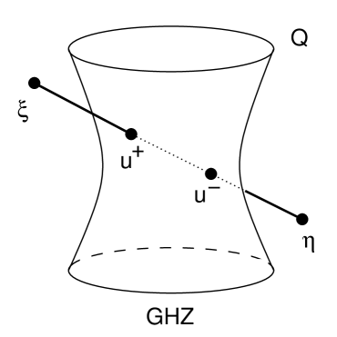
Figure 1: Geometric representation of large black holes corresponding to real states in the GHZ class. The line is defined by the vectors $\xi$ and $\eta$ of Eq. (86) defined by the dyonic charges. The points of intersection of the line with the quadric ${\cal Q}$ are the principal null directions $u^{\pm}$ defined by the frozen value of the moduli $S$ Eq. (76) on the horizon.

If the equation $Q(w\xi-\eta,w\xi-\eta)=0$ has merely one solution (the case of one principal null direction) the line is tangent to the quadric ${\cal Q}$ at this particular point. This can happen iff $D=0$ i.e. ${\tau}_{ABC}=0$. Then states belong to the W-class iff the corresponding lines are tangent to the quadric. After specializing again to real states now representing the small black holes we obtain the geometric situation depicted by Fig. 2.

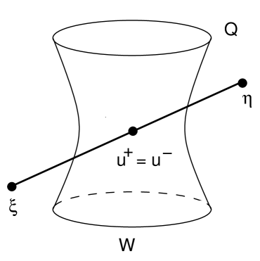
Figure 2: Geometric representation of small black holes corresponding to real states in the W class. The line is defined by the vectors $\xi$ and $\eta$ defined by the dyonic charges. The point of intersection of the line tangent to the quadric ${\cal Q}$ corresponds to the two coincident principal null directions $u^{\pm}$.

Note, however that in these two cases of genuine three-qubit entanglement the points through which the lines were defined are themselves not lying on ${\cal Q}$.

The next special case is the one of $A(BC)$ separable states. In this case ${\tau}_{A(BC)}=0$ hence according to Eq. (11) the vectors $\xi$ and $\eta$ are proportional, hence our line degenerates to a point not lying on the quadric ${\cal Q}$. Including also the degenerate case when one of the vectors e.g. $\eta$ is vanishing, we can represent the corresponding situation of small black holes by drawing a point off the quadric represented by the vector $\xi$ now with integer components (see Fig. 3).

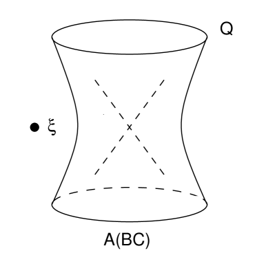
Figure 3: Geometric representation of small black holes corresponding to real states in the A(BC) class. The point off the quadric ${\cal Q}$ is defined by the vector $\xi$ of dyonic charges. The other vector $\eta$ is either projectively equivalent to $\xi$ or vanishing. The dashed lines intersecting at a point refer to the existence of two families of lines on ${\cal Q}$ ruling it.

Let us now turn to the cases when the lines themselves are lying inside the quadric ${\cal Q}$. Such lines are called isotropicHughston with respect to ${\cal Q}$. It is well-known that there are exactly two families of lines on a nondegenerate quadric ${\cal Q}$ in ${\bf CP}^{3}$. In other words our quadric ${\cal Q}$ is ruled by two families of lines. They are conventionally called $\alpha$-lines and ${\beta}$-linesHughston . Two of such representative lines are depicted in Fig. 3. Two lines belonging to the same family do not intersect; whereas, two lines belonging to the opposite families intersect at a single point (see Fig. 3.) on ${\cal Q}$. Hence any nondegenerate quadric in ${\bf CP}^{3}$ is isomorphic to ${\bf CP}^{1}\times{\bf CP}^{1}$. Using the results of our previous paperLevay1 one can show that these isotropic lines correspond precisely to $B(AC)$ and $C(AB)$ separable states. In order to see this recall thatLevay1 by defining ${\tau}_{+}={\tau}_{C(AB)}$ and ${\tau}_{-}={\tau}_{B(AC)}$ we have

$${\tau}_{\pm}=|\xi\cdot\xi|^{2}+2|\xi\cdot\eta|^{2}+|\eta\cdot\eta|^{2}+(P^{IJ}\mp\ast P^{IJ})\overline{P}_{IJ},$$ (90)

where

$$\ast P_{IJ}\equiv\frac{1}{2}{\varepsilon}_{IJKL}P^{KL},$$ (91)

and see Eq. (5) for the definition of the Plücker coordinates. Isotropic lines satisfy the relations $\xi\cdot\xi=\eta\cdot\eta=\xi\cdot\eta=0$, moreover such lines are necessarily self-dual or anti-self-dualHughston . Hence for isotropic lines we have either ${\tau}_{+}=0$ or ${\tau}_{-}=0$. Conversely, using the positivityLevay1 of the terms in Eq. (90) the vanishing of ${\tau}_{\pm}$ implies that the corresponding lines are isotropic. Since the states are C(AB) or B(AC) separable if and only if ${\tau}_{+}$ or ${\tau}_{-}$ vanishes, isotropic lines on ${\cal Q}$ represent precisely two of our biseparable classes. Specializing again to real states of $C(AB)$ or $B(AC)$ separable form representing small STU black holes we have the geometrical situation of Figs. 4 and 5.

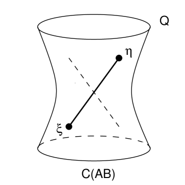
Figure 4: Geometric representation of small black holes corresponding to real states in the $C(AB)$ class. The line through the points $\xi$ and $\eta$ lying now on ${\cal Q}$ is an isotropic line, i.e. it lies entirely inside the quadric and coincides with one from the family of special lines of ${\cal Q}$. These lines are related to the self-duality of the Plücker matrix and are called $\alpha$-lines.

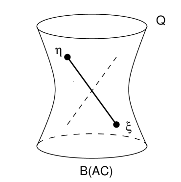
Figure 5: Geometric representation of small black holes corresponding to real states in the $B(AC)$ class. The line through the points $\xi$ and $\eta$ lying now on ${\cal Q}$ is an isotropic line, coinciding with one from the other family of special lines of ${\cal Q}$. These lines are related to the anti-self-duality of the Plücker matrix and are called $\beta$-lines.

Finally we are left with the geometrical representation of the small black holes corresponding to the totally separable class, i.e. the states of the form $(A)(B)(C)$. Such states are represented by points since they are $A(BC)$ separable, moreover they have to lie on the quadric since due to $C(AB)$ and $B(AC)$ separability they are parts of isotropic lines. The only possible way of representing them is by a point on the quadric which is of course located at the intersection of an $\alpha$ and a $\beta$-plane (see Fig. 6).

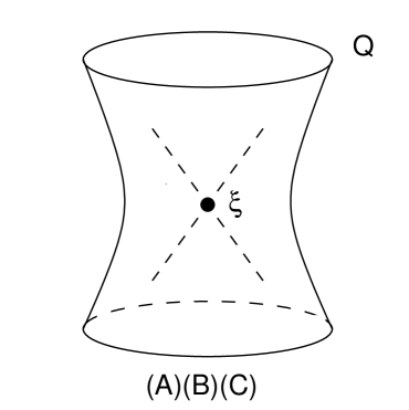
Figure 6: Geometric representation of small black holes corresponding to real states in the totally separable $(A)(B)(C)$ class. Such holes are represented by a single point lying at the intersection of an $\alpha$ and a $\beta$-line. Here this point is represented by $\xi$. The other point ${\eta}$ is either projectively equivalent to ${\xi}$ or can be taken to be zero.

Note that this geometrical representation is from the viewpoint of system $A$ or which is the same the $S$-part of the STU model. The fixed quadric ${\cal Q}$ is defined by using the $SL(2,{\bf R})\otimes SL(2,{\bf R})$ invariant metric Eq. (7). Since the symmetry of the STU model is $[SL(2,{\bf R})/SO(2)]^{\otimes 3}$ (the moduli are coordinates of this manifold) this choice of ${\cal Q}$ is dictated by the basic structure of the STU model. Physically however, all parties are equivalent hence the geometric picture as given by Figs. 1-6. is independent from the choice of parties. We can give however, to the subsystem $A$ a physically different role by allowing transformations on the combined system $BC$ (i.e. $TU$) of more general type. For example instead of applying the real version of the SLOCC group $SL(2,{\bf R})^{\otimes 3}$ we can have the larger one $SL(2,{\bf R})\otimes SO(2,2)$. This means that $B$ and $C$ are sharing among each other local resources of a more general kind than $A$. This enlargement of the SLOCC group in the entanglement picture amounts to using a dual description of black holes where the moduli $S$ is singled out and whose imaginary part plays the role of the string coupling constantRahmfeld ; Shmakova ; Kallosh . The manifold for the moduli in this picture is $\frac{SL(2,{\bf R})}{SO(2)}\times\frac{SO(2,2)}{SO(2)\times SO(2)}$. The different roles the parties $A$ and $BC$ play in the local protocols performed by them corresponds to the different characters $S$-duality and $T$ and $U$ dualities have in string theory. Indeed $S$-duality ( associated with the $SL(2,{\bf Z})$ subgroup of $SL(2,{\bf R})$) in this picture is of nonperturbative whereas $T$ and $U$ dualities based on $SO(2,2)$ symmetry are of perturbative character (i.e. they are not mixing electric and magnetic charges). This point has been emphasized by Kallosh and LindeLinde .

In our geometric representation this dual picture means that now Figs 1-6. repesent the physical situation of $S(TU)$ black holes. Althoug the nondegenerate quadric ${\cal Q}$ is now represented differently (i.e. in the $SO(2,2)$ form) the intersection properties are invariant. The choice of base describing the situation is the one obtained after applying an $Sp(8,{\bf R})$ transformation to the chargesShmakova which is in our labelling of the three-qubit system is equivalent to the $O(4,{\bf R})$ transformation

$$\hat{p}^{I}=\begin{pmatrix}\hat{p}^{1}\\ \hat{p}^{2}\\ \hat{p}^{3}\\ \hat{p}^{4}\end{pmatrix}=\frac{1}{\sqrt{2}}\begin{pmatrix}{\xi}_{1}-{\xi}_{4}\\ {\xi}_{2}+{\xi}_{3}\\ -{\xi}_{1}-{\xi}_{4}\\ -{\xi}_{2}+{\xi}_{3}\end{pmatrix}$$ (92)

$$\hat{q}^{I}=\begin{pmatrix}\hat{q}^{1}\\ \hat{q}^{2}\\ \hat{q}^{3}\\ \hat{q}^{4}\end{pmatrix}=\frac{1}{\sqrt{2}}\begin{pmatrix}{\eta}_{1}-{\eta}_{4}\\ {\eta}_{2}+{\eta}_{3}\\ -{\eta}_{1}-{\eta}_{4}\\ -{\eta}_{2}+{\eta}_{3}\end{pmatrix},$$ (93)

where now indices are lowered with the $SO(2,2)$ invariant metric $h_{IJ}={\rm diag}(-1,-1,+1,+1)$. Clearly $\hat{p}^{I}\hat{q}_{I}=h_{IJ}\hat{p}^{I}\hat{q}{J}=\xi\cdot\eta$, see Eq. (89). In closing this section we note that the choice of base Eqs. (92) and (93) corresponds to the real version of the so called magic base of Hill and Wootters Wootters , which is related to the usual conversion of four-vector indices to spinorial ones of twistor theoryPenrose .

V Conclusions

In this paper we have studied intresting similarities between two different fields of theoretical physics, quantum information theory and the physics of stringy black holes. Though they are seemingly unrelated, one can realize that the unifying themes in both of these fields such as information, entropy, and entanglement are the same. Since the near horizon geometry of black holes is $AdS^{2}\times S^{2}$ using the idea of Ads/CFT holography one might certainly expect connections between entanglement entropy and black hole entropy. Though there are some interesting recent developmentsBrustein in relating entanglement entropy and black hole entropy, the correspondence between these notions is not well-understood. In order to get some further insight into the nature of such important problems it is sometimes useful to look for the clues coming from different strains of knowledge. Hence, following the initiative of DuffDuff and Kallosh and Linde Linde in the present paper we have established new relations between extremal black holes in the $STU$-model of string theory and qubit systems in quantum information theory.

In particular we have shown that the well-known process of finding the frozen values for the moduli on the horizon in the theory of STU black holes corresponds to the problem of finding a canonical form for the three qubit state defined by the dyonic charges using ${\it complex}$ SLOCC transformations in quantum information theory. Alternatively, this process equivalent to solving the stabilization (attractor) equations in one picture corresponds to obtaining the optimal distillation protocol for a GHZ-state in the other. The geometric representation for this process was found. It is equivalent to finding the principal null directions of a complex plane in ${\bf C}^{4}$. We have managed to characterize geometrically the real states describing STU black holes by embedding them inside the more general complex ones used in quantum information theory. Using the language of twistors based on the intersection properties of complex lines with a fixed quadric ${\cal Q}$ in ${\bf CP}^{3}$ an instructive geometric classification for STU black holes was given.

Let us now add some important observations to these results. Let us first consider the transformed state of Eq. (61). As we have shown using the frozen values for the moduli $S$, $T$ and $U$ results in the state of the $GHZ$ form Eq. (82). Since the amplitudes of this state besides ${\psi}^{\prime}_{000}$ and ${\psi}^{\prime}_{111}$ are zero the projection onto these components in Eq. (60) is not needed. Hence $M^{2}_{BPS}|_{\rm extr}=\frac{1}{2}{||{\psi}^{\prime}||^{2}}_{\rm hor}=\frac{1}{2}\langle\psi|C_{U}^{\dagger}C_{U}\otimes B_{T}^{\dagger}B_{T}\otimes A_{S}^{\dagger}A_{S}|\psi\rangle_{\rm hor}$. Then we get for the black hole entropy

$$S_{BH}=\frac{\pi}{2}{||{\psi}^{\prime}||^{2}}_{\rm hor}=\frac{\pi}{2}\sqrt{{\tau}_{ABC}}.$$ (94)

This interesting formula relates the black hole entropy to the value of the norm of the transformed state at the horizon. Now in papersAcin3 ; Verstr the optimal local distillation protocol for the canonical GHZ state $\frac{1}{\sqrt{2}}(|000\rangle+|111\rangle)$ was found. In particular it was provedVerstr that the total probability for obtaining the canonical GHZ state is bounded from above by $\sqrt{{\tau}_{ABC}}/{\lambda}_{max}(C^{\dagger}C\otimes B^{\dagger}B\otimes A^{\dagger}A)$. Here ${\lambda}_{max}(X)$ denotes the largest eigenvalue of the operator $X$ and the parameter dependent operators $A,B,C$ are the generalizations of our $A_{S},B_{T},C_{U}$ of Eq. (59) for the complex case. Hence an upper bound is achieved by minimizing this largest eigenvalue with respect to the parameters. These observations show that in the case of BPS STU black holes the minimum area principle of the supersymmetric attractor mechanism is somehow related to the maximization of the probability of success for converting a particular state to the canonical GHZ state . It would be interesting to use the insight and formalism provided by stringy black holes for obtaining an alternative description of this optimization process.

As our second observation let us consider the real state

$$|\hat{\psi}(S,T,U)\rangle\equiv{\cal C}_{U}\otimes{\cal B}_{T}\otimes{\cal A}_{S}|\psi\rangle,$$ (95)

known from Eq. (54). Then it is easy to show that

$$\langle\hat{\psi}|{\sigma}_{2}\otimes{\sigma}_{2}\otimes I|\hat{\psi}\rangle={\rm Tr}(\hat{\varrho}_{BC}{\sigma}_{2}\otimes{\sigma}_{2}),$$ (96)

where now $\hat{\varrho}_{BC}(S,T,U)\equiv\hat{\psi}_{lk0}\hat{\psi}_{l^{\prime}k^{\prime}0}+\hat{\psi}_{lk1}\hat{\psi}_{l^{\prime}k^{\prime}1}=\hat{\xi}_{I}\hat{\xi}_{J}+\hat{\eta}_{I}\hat{\eta}_{J}$ (compare with Eq. (15)). Using similar manipulations for the expectation values of the operators ${\sigma}_{2}\otimes I\otimes{\sigma}_{2}$ and $I\otimes{\sigma}_{2}\otimes{\sigma}_{2}$ we obtain for the BPS mass squared Eq. (54) the formula

$$M_{BPS}^{2}=\frac{1}{8}(||\hat{\psi}||^{2}+{\rm Tr}(\hat{\varrho}_{BC}{\sigma}_{2}\otimes{\sigma}_{2})+{\rm Tr}(\hat{\varrho}_{AC}{\sigma}_{2}\otimes{\sigma}_{2})+{\rm Tr}(\hat{\varrho}_{AB}{\sigma}_{2}\otimes{\sigma}_{2})).$$ (97)

Now in Ref. 17. it was shown that the magnitudes ${\cal C}_{BC}\equiv|{\rm Tr}(\hat{\varrho}_{BC}{\sigma}_{2}\otimes{\sigma}_{2})|$ etc. define the concurrences for the real qubits i.e. rebits. Moreover, this quantity defines the important quantity, the entanglement of formation for rebits via the formula

$$E(\hat{\varrho}_{BC})=H\left(\frac{1+\sqrt{1-{\cal C}^{2}(\hat{\varrho}_{BC})}}{2}\right)$$ (98)

where $H(x)=-x\log_{2}x-(1-x)\log_{2}(1-x)$ is the binary Shannon entropy. Since $|\hat{\psi}\rangle$ and $|{\psi}^{\prime}\rangle$ are unitarily related (see Eq. (56)) we have $||\hat{\psi}||^{2}=||{\psi}^{\prime}||^{2}$ hence the extremal BPS mass squared can also be written in the form ${M^{2}_{BPS}}|_{\rm extr}=\frac{1}{2}\overline{\cal C}_{\rm hor}$ where $\overline{\cal C}=\frac{1}{3}({\cal C}_{AB}+{\cal C}_{BC}+{\cal C}_{AC})$ is the average real concurrence. Hence the entropy for the large BPS STU black hole can be written in the alternative forms

$$S_{BH}=\frac{\pi}{2}\sqrt{\hat{\tau}_{ABC}}=\frac{\pi}{2}\overline{\cal C}_{\rm hor}=\frac{\pi}{2}||\hat{\psi}||^{2}_{\rm hor}.$$ (99)

Notice that in these expressions all quantities are expressed in terms of the real moduli dependent three-qubit state $|\hat{\psi}\rangle$ Eq. (95) calculated with the frozen values for them at the horizon. Of course due to the $SL(2,{\bf R})$ invariance of the three-tangle we have $\hat{\tau}_{ABC}={\tau}_{ABC}$ so it has the same value, no matter we use the state $|\psi\rangle$ with integer or the one $|\hat{\psi}\rangle$ with moduli dependent real amplitudes. However, the norm and the average real concurrence depends on the values of the moduli in a nontrivial way. Indeed, according to Eq. (97) the combination of these quantities gives $M_{BPS}^{2}$ to be extremized. However, quite remarkably all three quantities are frozen to the same value at the horizon.

The occurrence of the real concurrence (of which the real entanglement of formation is a monotonically increasing and convex function) in the STU black-hole scenario suggests a possibility for an alternative physical interpretation of the macroscopic black hole entropy. As it is well-known (see Ref. 34 for a nice review) the entanglement of formation of a two-qubit mixed state $\varrho$ is related to the minimum number of EPR pairs required to create that state $\varrho$. More precisely we have the following definition. Let us consider all pure state decompositions of the mixed state $\varrho$ of two qubits say $A$ and $B$ in the form $\varrho=\sum_{k=1}^{M}p_{k}|{\Phi}_{k}\rangle\langle{\Phi}_{k}\rangle$. Let us moreover introduce the quantity $E(\Phi)=S({\rm Tr}_{B}|\Phi\rangle\langle\Phi|)=S({\rm Tr}_{A}|\Phi\rangle\langle\Phi|)$ with $S$ denoting the von Neumann entropy. Then the definition of the entanglement of formation isWootters ; Wootters2

$$E(\varrho)={\rm inf}\sum_{k}p_{k}E({\Phi}_{k}),$$ (100)

where the infimum is taken over all pure state decompositions of $\varrho$. These definitions and Eq. (99) clearly shows the possibility of relating the BPS STU black hole entropy to the minimization of the number of EPR pairs needed to create a state characterized by the density matrices $\hat{\varrho}_{AB}$, $\hat{\varrho}_{BC}$ and $\hat{\varrho}_{AC}$ as a function of the moduli fields. This number according to the very definition of the entanglement of formation Eq. (100) is also related to the minimization of the convex hull of the von-Neumann entropies with respect to all possible pure state decompositions of the state ${\varrho}$. This idea relating the average entanglement of formation to the black hole entropy might turn out to be relevant in identifying the black hole entropy with the entanglement entropy within the framework of AdS/CFT correspondence.

It is important to interpret the message of these sentences correctly. The entanglement present in the physics of STU black holes is of unusual type. Here the entanglement is not carried by distinguishable particles as in quantum information theory, but rather by special nonlocal objects that are composites of quantized charges and the moduli (see Eq. (95)). Indeed the real entangled state of Eq. (95) is represented by an entire line in our geometric representation. Then when we are talking about entanglement of formation using EPR pairs etc. one has to have in mind this strange kind of entanglement. Of course according to the microscopic interpretation of black hole entropy since the quantized charges are relatedLinde to the numbers of $D0$, $D2$, $D4$, and $D6$ branes this kind of entanglement somehow should boil down to the usual one of string theory states.

Returning back to the real concurrence, we stress that its square is not the same as the restrictions of the squares of the complex concurrences , i.e. the quantities ${\tau}_{AB}$, ${\tau}_{BC}$ and ${\tau}_{AC}$ to the real domain. In fact it is easy to show that for BPS STU black holes i.e. $D<0$ we have

$${\cal C}^{2}_{AB}={\tau}_{AB}+{\tau}_{ABC}.$$ (101)

However, for non-BPS STU black-holes i.e. $D>0$ the two concepts turn out to be identical, i.e. in this case we have for example ${\cal C}^{2}_{AB}={\tau}_{AB}$. Looking back at the form of our reality conditions Eqs. (29) and (30) it is clear that using the notion of the real concurrence these expressions can be cast into a unified form. For example the reality condition for BPS STU black holes is ${\sigma}_{ABC}={\cal C}_{AB}{\cal C}_{BC}{\cal C}_{AC}$.

These considerations and the geometric representation of Section IV. shows that the three-qubit states relevant to STU black holes are described by real lines in ${CP}^{3}$. These lines are lying on $SU(2)^{\otimes 3}$ orbits of the ones determined by the vectors ${\xi}$ and ${\eta}$ defined by the dyonic charges or of the more general ones determined by the ones $\hat{\xi}$ and ${\hat{\eta}}$ corresponding to the moduli dependent real states $|\hat{\psi}\rangle$. In this paper we have used the complex geometry of three-qubit states of the most general type. However, the three-qubit states having some relevance for stringy black holes are at most real. Though we have clarified how these states are embedded in the space of the most general three-qubit ones the question arises, is there any relevance to string theory the existence of complex three-qubit states of the most general kind? Though we do not know the answer, we note that the situation is somewhat similar to the one in twistor theory. In twistor theoryPenrose ; Ward ; Hughston real lines (defined differently than here) in ${\bf CP}^{3}$ correspond to points of conformally compactified Minkowski space time, however to see the full power of twistor geometry one is forced to include also complex lines corresponding to points of complexified and compactified Minkowski space time. This Klein correspondence where instead of lines in ${\bf CP}^{3}$ points in a space (the complex Grassmannian Gr(2,4)) isomorphic to compactified and complexified Minkowski space-time can be used to obtain a geometrical representation for three-qubit states similar to the one presented hereLevay1 . Notice that this correspondence between lines and space-time points is a non local one, which according to the original motivation of twistor theory is expected to play an important role in describing the nonlocality of quantum entanglement.

Though the similarity between the real lines found here and the ones of twistor theory is obvious it is not at all clear how can we relate these geometric considerations to the underlying special geometry of $N=2$, $D=4$ supergravity or to string theory states with some number of $D$-branes. Note, however that the special role of real coordinates (the analogue of our real lines found here) in supergravity theories is currently under investigationMohaupt ; Macia . For the moment the status of the new relations found in this paper is just like the ones of Refs. [10,13] that they are merely mathematical coincidences. Though we are aware that the appearance of a mathematical structure in two disparate subjects does not necessarily imply a deeper unity, the realization that these relations do exist might turn out to be important for obtaining further insights for both string theorists and researchers working in the field of quantum information.

VI Acknowledgements

Financial support from the Országos Tudományos Kutatási Alap (OTKA), (grant numbers T032453 and T038191) is gratefully acknowledged. We also thank Dr. László Borda for his help with the figures.

References

- (1) E. Schrödinger, Proceedings of the Cambridge Philosophical Society, 31, 555 (1935).
- (2) C. H. Bennett, G. Brassard, C. Crépeau, R. Jozsa, A. Peres, and W. K. Wootters, Phys. Rev. Lett. 70, 1895 (1993).
- (3) C. H. Bennett and D. P. DiVincenzo, Nature (London) 404, 247 (2000).
- (4) M. A. Nielsen and I. L. Chuang, Quantum Computation and Quantum Information (Cambridge University Press, Cambridge, 2000).
- (5) S. Ferrara, R. Kallosh and A. Strominger, Phys. Rev. 52 5412 (1995), A. Strominger, Phys. Lett B 383 39 (1996), S. Ferrara and R. Kallosh, Phys. Rev. D 54, 1514 (1996).
- (6) A. Strominger and C. Vafa, Phys. Lett. B 379, 99 (1995).
- (7) C. M. Hull and P. K. Townsend, Nucl. Phys. B 348, 109, (1995).
- (8) E. Witten, Nucl. Phys. B 443, 85 (1995).
- (9) J. Polchinski, Phys. Rev. Lett. 75 4724 (1995).
- (10) M. Duff, hep-th/0601134.
- (11) I. M. Gelfand, M. M. Kapranov, A. V. Zelevinsky, Discriminants, resultants and multidimensional determinants, Birkhäuser Boston 1994.
- (12) V. Coffman, J Kundu and W. K. Wootters, Phys. Rev. A 61 052306 (2000).
- (13) R. Kallosh and A. Linde, hep-th/0602061
- (14) P. Lévay, Phys.Rev. A 71, 012334 (2005), quant-ph/0403060
- (15) R. Penrose and W. Rindler, Spinors and Space-Time, Vols.1-2. Cambridge University Press, 1984.
- (16) R. S. Ward, R. O. Wells jr., Twistor geometry and field theory , Cambridge monographs on mathematical physics (1990).
- (17) C. M. Caves, C. A. Fuchs, and P. Rungta, Foundations of Physics Letters 14 199 (2001), quant-ph/0009063.
- (18) K. Behrndt, R. Kallosh, J. Rahmfeld, M. Shmakova and W. K. Wong, Phys. Rev. D 54 6293 (1996).
- (19) W. Dür, G. Vidal, and J. I. Cirac, Phys. Rev. A 62, 062314 (2000).
- (20) N. Gisin and H. Beschmann-Pasquinucci, Phys. Lett. A 246 1 (1998).
- (21) P. Lévay, J. Phys. A 38, 9075 (2005).
- (22) S. Hill and W. Wootters, Phys. Rev. Lett. 78, 5022 (1997).
- (23) T. Sudbery, J. Phys. A 34, 643 (2001).
- (24) A. Acin, A. Andrianov, L. Costa, E. Jané, J. I. Latorre and R. Tarrach, Phys. Rev. Lett. 85, 1560 (2000).
- (25) A. Acin, A. Andrianov, E. Jané and R. Tarrach, J. Phys. A 34 6725 (2001).
- (26) B. de Wit, P. G. Lauwers and A. Van Proeyen, Nucl. Phys. B 255 568 (1985).
- (27) R. Kallosh, M. Shmakova and W. K. Wong, Phys. Rev. D 54 6284 (1996).
- (28) A. Strominger, Commun. Math. Phys. 133 163 (1990).
- (29) M. J. Duff, J. T. Liu and J. Rahmfeld, Nucl. Phys. B 459 125 (1996).
- (30) L. P. Hughston and T. R. Hurd, Physics Reports 100, 273 (1983).
- (31) R. Brustein. M. B. Einhorn and A. Yarom, JHEP 0601 098 (2006), S. Ryu and T. Takayanagi, hep-th/0603001, R. Emparan, hep-th/0603081.
- (32) A. Acin, E. Jané, W. Dür, and G. Vidal, Phys. Rev. Lett. 22 4811 (2000).
- (33) F. Verstraete, J. Dehaene and B. De Moor, Phys. Rev. A65 032308 (2002).
- (34) W. K. Wootters, Quantum Information and Computation, Vol 1. 27 (2001).
- (35) T. Mohaupt, New developements in special geometry, hep-th/0602171.
- (36) S. Ferrara and O. Maciá, Observations on the Darboux coordinates for rigid special geometry,hep-th/0602262.