Inflating in a Better Racetrack

Abstract:

We present a new version of our racetrack inflation scenario which, unlike our original proposal, is based on an explicit compactification of type IIB string theory: the Calabi-Yau manifold ${\rm I\kern-1.79993ptP}^{4}_{[1,1,1,6,9]}$. The axion-dilaton and all complex structure moduli are stabilized by fluxes. The remaining 2 Kähler moduli are stabilized by a nonperturbative superpotential, which has been explicitly computed. For this model we identify situations for which a linear combination of the axionic parts of the two Kähler moduli acts as an inflaton. As in our previous scenario, inflation begins at a saddle point of the scalar potential and proceeds as an eternal topological inflation. For a certain range of inflationary parameters, we obtain the COBE-normalized spectrum of metric perturbations and an inflationary scale of $M=3\times 10^{14}$ GeV. We discuss possible changes of parameters of our model and argue that anthropic considerations favor those parameters that lead to a nearly flat spectrum of inflationary perturbations, which in our case is characterized by the spectral index $n_{s}=0.95$.

1 Introduction

The past two years have seen continued progress in identifying how cosmological inflation can arise from within string theory. Several interesting mechanisms have been examined so far, including brane/antibrane inflation [1]–[7], D3/D7 brane inflation [8], DBI inflation [9], tachyon inflation [10] and inflation driven by various kinds of closed-string moduli [11]–[14] or more stringy degrees of freedom [15]. There is continued interest in identifying where inflation can arise within the enormous landscape of string configurations.

The Racetrack Inflation scenario of Ref. [12] gives a particularly simple scenario, based on a Calabi-Yau compactification of type IIB string theory having only a single Kähler modulus once fluxes are used to fix the complex-structure moduli. It was argued that the one remaining Kähler modulus could be the inflaton provided the nonperturbative superpotential for this modulus has a double-exponential form, known in the literature as a racetrack model [16]. For appropriate choices of the parameters of this superpotential this model can give rise to standard hill-top, topological slow-roll inflation. This is in contrast with the simplest single-exponential case originally discussed in the KKLT model [17], which does not similarly give rise to inflation.

Even though very simple and predictive, a drawback with this scenario is the absence of an explicit string construction which produces the required racetrack superpotential. More generally, it remains a challenge to derive inflation within an explicit string configuration for which all of the features of the complete potential which stabilize the moduli are explicitly calculable.

In this paper we identify how inflation can be obtained using the low-energy field theory which is known to describe the two Kähler moduli of the ${\rm I\kern-1.79993ptP}^{4}_{[1,1,1,6,9]}$ model, for which Denef, Douglas and Florea were able to provide explicit calculations of the nonperturbative superpotential [18]. The title of their paper — “Building a Better Racetrack” — explains the title of ours. We should note, however, that although the superpotential they find is a sum of two exponentials, it differs from the usual racetrack superpotential because each exponential depends only on a different Kähler modulus. We find that the resulting scalar potential can nevertheless produce inflation in a racetrack-like way: through the slow-roll of a linear combination of the Kähler moduli axions away from a local saddle point towards a nearby local minimum.

We describe these results in the following way. Section 2 starts with a brief summary of the original racetrack-inflation mechanism for a single modulus, followed in Section 3 by a description of its generalization to the two-modulus case of interest for the ${\rm I\kern-1.79993ptP}^{4}_{[1,1,1,6,9]}$ type IIB vacuum. In Section 4 we describe a particular choice of parameters which lead to eternal topological inflation in this model. In Section 5 we describe the derivation of the amplitude of the spectrum of scalar metric perturbations in our model. In Section 6 we discuss a relation between our parameters, the flatness of the spectrum, and the total duration of inflation, and argue that anthropic considerations show some preferences for the parameters leading to the flat spectrum. Our conclusions are then discussed in Section 7.

2 Single-Modulus Racetrack Inflation

In this section we briefly review the original proposal for racetrack inflation within the KKLT scenario [12]. This scenario is based on those vacua of type IIB string theory which are obtained by compactifying to 4 dimensions in an $N=1$ supersymmetric way on an orientifolded Calabi-Yau manifold in the presence of three-form RR and NS fluxes and D7 branes. The presence of the fluxes can fix the values of the complex dilaton field and of the various complex-structure moduli of the underlying Calabi-Yau space [19, 20], leading to a low-energy 4D supergravity describing the remaining Kähler moduli which has the no-scale form [21], for which the remaining moduli correspond to exactly flat directions of the scalar potential.

2.1 Vacuum Solutions

Explicitly, the potential for these moduli is given by the standard $N=1$ F-term potential of $N=1$ supergravity, which in Planck units reads

$$V_{F}~{}=~{}e^{K}\left(K^{i\bar{\jmath}}D_{i}W\overline{D_{j}W}-3|W|^{2}\right)\,,$$ (1)

with $i,j$ running over the various complex chiral fields, $\varphi^{i}$. $K^{i\bar{\jmath}}$ denotes the inverse of the matrix $K_{i\bar{\jmath}}=\partial_{i}\partial_{\bar{\jmath}}K$, and the Kähler covariant derivative is $D_{i}W=\partial_{i}W+(\partial_{i}K)W$, where $K$ is the system’s Kähler potential and $W$ its superpotential. For the low-energy moduli obtained from a flux compactification typically $W=W_{0}$ depends only on the complex-structure moduli, and is therefore a constant so far as the Kähler moduli are concerned. The Kähler function for the Kähler moduli also satisfies the no-scale identity

$$K^{i\bar{\jmath}}K_{i}{K_{j}}=3\,,$$ (2)

implying that $V_{F}=0$; hence these moduli are not fixed by the fluxes themselves.

In order to fix all moduli KKLT imagined starting with a Calabi-Yau space having just a single Kähler modulus, the volume modulus $T$. For this the Kähler potential $K$, obtained neglecting possible corrections in powers of $\alpha^{\prime}$ and the string coupling has been computed to have the no-scale form [24]

$$K=-3\log(T+T^{*})\,.$$ (3)

The flat direction in the $T$ direction is lifted once $W$ acquires a $T$-dependence, such as can be generated by D3-instantons, or gaugino condensation if a suitable gauge sector exists on one of the D7 branes.

Writing the field $T$ in terms of its real and imaginary parts,

$$T\,\equiv X+iY\,,$$ (4)

and using (1) and (3), the supersymmetric part of the scalar potential turns out to be

$$V_{F}=\frac{1}{8X^{3}}\left\{\frac{1}{3}\left|2XW^{\prime}-3W\right|^{2}-3|W|^{2}\right\}\,,$$ (5)

where ^′ denotes differentiation with respect to $T$. The supersymmetric minima of this potential are given by the solutions of

$$2XW^{\prime}-3W=0\,,$$ (6)

for which it is clear that the value of the potential at the minimum is generically negative, leading to vacua with 4D anti-de Sitter geometry.

KKLT obtain metastable vacua having de Sitter geometry in four dimensions by raising the potential at this minimum to positive values by introducing anti-D3 branes. The presence of these branes does not introduce extra translational moduli since their positions are fixed by the fluxes [25], and so their low-energy effect is just a contribution to the energy density of the system. Provided the antibrane tension is small — such as if they reside at the tip of a strongly-warped throat — it represents a small perturbation to the total energy density, and the 4D scalar potential which results is a sum of two parts

$$V=V_{F}+\delta V\,.$$ (7)

Here $\delta V$ represents the small, explicitly nonsupersymmetric, part of the potential induced by the tension of the anti-D3 branes.

Alternatively, this same lifting could be obtained by turning on magnetic fluxes on the D7 branes, and using the resulting Fayet-Iliopoulos D-term potential to raise the value of the potential at its minimum [26], again leading to a result of the form of eq. (7), with $\delta V$ being the D-term part of the potential induced by the magnetic field fluxes. In either case the form of $\delta V$ is positive definite and depends on an inverse power of the overall volume of the Calabi-Yau space,

$$\delta V=\frac{E}{X^{\alpha}}\,.$$ (8)

for constants $E,\alpha>0$. The coefficient $E$ is proportional to the antibrane tension, $T_{3}$, gravitationally redshifted by the local value of the warp factor. The exponent is $\alpha=2$ if $\delta V$ arises from anti-D3 branes sitting at the end of a Calabi-Yau throat, or if it arises from magnetic-field fluxes on D7 branes wrapped on cycles at the tip of such a throat. Otherwise $\alpha=3$, corresponding to anti-D3 branes (or magnetic flux on D7 branes) situated in an unwarped region. For anti-D3 branes the warped region is energetically preferred and so in what follows we take $\alpha=2$.

Further progress requires specifying the $T$-dependence of the superpotential, for which KKLT take the simplest form:

$$W=W_{0}+A\,e^{-aT}\,.$$ (9)

This choice allows minima for $V_{F}$ at large $X$ — as is required by the supergravity approximation to string theory — provided the fluxes are arranged to ensure that $W_{0}$ is sufficiently small. (In the limit $W_{0}\to 0$ the minima disappear, leading instead to a runaway potential.) The analysis also goes through for more complicated possibilities for $W$, however, such as if $W$ were given by modular functions as would be expected for $N=2^{*}$ models [27], or if it involved the sum of two exponentials [12]

$$W=W_{0}+A\,e^{-aT}+B\,e^{-bT}\,.$$ (10)

This last superpotential includes the original KKLT scenario if $AB=0$ and has the property that it can naturally provide minima for $V_{F}$ which lie in the large-field region. (When $W_{0}=0$ the superpotential of eq. (10) reduces to the standard racetrack form, which was studied in the past as a superpotential which could stabilize the dilaton field at weak coupling for heterotic string vacua [16].) Such a superpotential arises when gauginos condense for a supersymmetric gauge theory (with no charged matter) involving a product gauge group. For instance, the gauge group $SU(N)\times SU(M)$ leads to a sum of exponentials with both $A$ and $B$ nonzero, while $a=2\pi/N$ and $b=2\pi/M$ [28]. Minima at large $X$ are then generic for large values of $N$ and $M$, with $M$ close to $N$.

In terms of the real component fields the supersymmetric part of the potential obtained using the superpotential (10) takes the following form (for real $W_{0}$):

$$V_{F} = \frac{e^{-(a+b)X}}{6X^{2}}\Bigl{\{}aA^{2}\left(aX+3\right)~{}e^{(b-a)X}+bB^{2}\left(bX+3\right)\,e^{-(b-a)X}$$

$$\qquad\qquad+AB\left(2abX+3a+3b\right)\cos[\left(a-b\right)Y]$$

$$\qquad\qquad\qquad+3W_{0}\left(aAe^{bX}\cos[aY]+bBe^{aX}\cos[bY]\right)\Bigr{\}}$$

The scalar potential obtained by summing this with $\delta V=E/X^{\alpha}$ has several de Sitter minima, depending on the values of the parameters $A,a,B,b,W_{0}$ and $E$. In general the different periodicities of the $Y$-dependent terms lead to a very rich landscape of vacua [27, 29]. This is particularly so if $a-b$ is taken to be very small (as is done for the standard racetrack models), such as if we take $a=2\pi/M$ and $b=2\pi/N$ with integers $N\sim M$ and both large.

The pattern of vacua obtained using (10) differs from that found with the original KKLT scenario in that it allows nontrivial minima even when $W_{0}=0$. For $W_{0}\neq 0$, many new local minima appear due to the small periodicity of the terms proportional to $W_{0}$ in the scalar potential. By choosing the background fluxes appropriately we have the freedom to adjust the values of $W_{0}$ and $E$. In particular $E$ can be tuned, as in KKLT, to adjust the value of the potential at its minimum. Unlike for the KKLT case, these parameters can also be adjusted to arrange the existence of local minima which are both supersymmetric and flat in four dimensions [29].

2.2 Inflationary Slow Roll

Another important difference between the superpotentials (9) and (10) is seen once one examines the dynamics of the field $T$ as it rolls towards these vacua. In particular, for inflationary purposes our interest is in slow rolls, for which the scalar-field energy is dominated by its potential rather than its kinetic energy. The main point of ref. [12] was that such slow rolls can exist for the superpotential (10), even though they do not for (9).

A sufficient condition for the occurrence of an inflationary slow roll is $\epsilon,|\eta|\ll 1$, where $\epsilon$ and $\eta$ are the slow-roll parameters [30], suitably generalized [6, 31] for scalars having nonminimal kinetic terms, ${\cal L}_{\rm kin}=-\frac{1}{2}\,g_{ab}(\phi)\partial_{\mu}\phi^{a}\partial^{\mu}\phi^{b}$. Explicitly, these are

$$\epsilon=\frac{1}{2}\left(\frac{g^{ab}\,\partial_{a}V\partial_{b}V}{V^{2}}\right)$$ (12)

while $\eta$ is defined as the most-negative eigenvalue of the matrix

$${N^{a}}_{b}=\left[\frac{g^{ac}(\partial_{c}\partial_{b}V-\Gamma^{d}_{cb}\partial_{d}V)}{V}\right]\,,$$ (13)

These definitions assume Planck units, and in them the indices ‘$a,b,c,d$’ run over a complete basis of fields, $\phi^{a}$. The connection, $\Gamma^{d}_{cb}(\phi)$, appearing in $\eta$ is constructed in the usual way from the target-space metric, $g_{ab}(\phi)$, which is in turn defined by the scalar-field kinetic terms. The point behind these definitions is their invariance under redefinitions of the scalar fields, and their reduction to the standard ones when evaluated for fields with minimal kinetic terms.

Notice also that the complications in $\eta$ having to do with the connection $\Gamma^{a}_{bc}$ are irrelevant when specialized to points for which $\epsilon$ vanishes.

The above expressions simplify when expressed in a complex field basis $\{\phi^{a}\}=\{\varphi^{i},\overline{\varphi}^{\bar{\jmath}}\}$, for which the target-space metric has components $g_{ij}=g_{\bar{\imath}\bar{\jmath}}=0$ and $g_{i\bar{\jmath}}=g_{\bar{\imath}j}=\partial_{i}\partial_{\bar{\jmath}}K$. In this case the only nonzero connection components are $\Gamma^{i}_{jk}=K^{i\bar{n}}\partial_{j}\partial_{k}\partial_{\bar{n}}K$ and their complex conjugates. The above definitions then reduce to

$$\epsilon=\left(\frac{K^{i\bar{\jmath}}\,\partial_{i}V\partial_{\bar{\jmath}}V}{V^{2}}\right)$$ (14)

and

$${N^{a}}_{b}=\left({\begin{array}[]{cc}{N^{i}}_{j}&{N^{i}}_{\bar{\jmath}}\\ {N^{\bar{\imath}}}_{j}&{N^{\bar{\imath}}}_{\bar{\jmath}}\end{array}}\right)\,,$$ (15)

where

$${N^{i}}_{k}=\frac{K^{i\bar{\jmath}}\partial_{\bar{\jmath}}\partial_{k}V}{V}\,,\qquad{N^{k}}_{\bar{\imath}}=\frac{K^{k\bar{\jmath}}(\partial_{\bar{\imath}}\partial_{\bar{\jmath}}V-K^{l\bar{n}}\partial_{\bar{\imath}}\partial_{\bar{\jmath}}\partial_{l}K\,\partial_{\bar{n}}V)}{V}\,,$$ (16)

and ${N^{\bar{\imath}}}_{\bar{\jmath}}$ and ${N^{\bar{k}}}_{i}$ are obtained from these by complex conjugation.

Usually a fine tuning of some of the parameters of the model are required in order to ensure that both $\epsilon$ and $|\eta|$ are sufficiently small. For instance for the superpotential (10) it was found in [12] that the potential has a saddle point (for which $\epsilon=0$) near a flat local minimum, but a tuning of the order of 1 part in 1000 was needed, in some of the parameters of the model, in order for $|\eta|$ to be small enough to obtain the minimal $60$ $e$-foldings of inflation ( See [12] for details.).

Once an inflationary region is obtained, the observed size of the CMB temperature fluctuations may be obtained by adjusting the string scale, typically leading to a value close to the GUT scale. The consistency of this with the observed value of Newton’s constant then implies a condition on the VEV of the volume modulus that determines the string scale from the Planck scale. Even though this procedure looks (and is) quite restrictive, solutions nonetheless exist having acceptable values for all of these experimentally measurable quantities. In refs. [6, 12] the scaling properties of the low-energy action were exploited in finding values of the parameters which satisfied all of these criteria.

3 The orientifold of ${\rm I\kern-1.79993ptP}^{4}_{[1,1,1,6,9]}$

We now return to the main line of development, and repeat the above steps for the orientifold of degree 18 hypersurface ${\rm I\kern-1.79993ptP}^{4}_{[1,1,1,6,9]}$, an elliptically fibered Calabi-Yau over $\mathbb{P}^{2}$. The stabilization of moduli in this model was performed in [18] where it was also shown how D3 instantons generate a nonperturbative superpotential, thus providing an explicit realization of the KKLT scenario.

The model is a Calabi-Yau threefold with the number of Kähler moduli $h^{1,1}=2$ and the number of complex structure moduli $h^{2,1}=272$. The 272 parameter prepotential for this model is not known. We will restrict ourselves to the slice of the complex structure moduli space which is fixed under the action of the discrete symmetry $\Gamma\equiv\mathbb{Z}_{6}\times\mathbb{Z}_{18}$. This allows to reduce the the moduli space of the complex Calabi-Yau structures to just 2 parameters, since the slice is two-dimensional. This restricted model has a long string pedigree, starting with [32]; it is a hypersurface in the weighted projective space ${\rm I\kern-1.79993ptP}^{4}_{[1,1,1,6,9]}$. The remaining 270 moduli are required to vanish to support this symmetry. The defining equation for the Calabi-Yau 2-parameter subspace of the total moduli space is

$$f=x_{1}^{18}+x_{2}^{18}+x_{3}^{18}+x_{4}^{3}+x_{5}^{2}-18\psi x_{1}x_{2}x_{3}x_{4}x_{5}-3\phi x_{1}^{6}x_{2}^{6}x_{3}^{6}\,.$$ (17)

The first stage of the GKP-KKLT scenario [19, 17], stabilization of the type IIB axion-dilaton $\tau$ and the two complex structure moduli $\psi$ and $\phi$ in eq. (17) was performed in [18] explicitly. It was important at this stage to turn on only the fluxes on $\Gamma$-invariant cycles, the same tool has been used in other models of flux vacua stabilization in [33].

The Kähler geometry of the remaining two Kähler moduli $h^{1,1}=2$ was specified in [32, 18]. We denote them by $\tau_{1,2}=X_{1,2}+iY_{1,2}$. These moduli correspond geometrically to the complexified volumes of the divisors (or four-cycles) $D_{4}$ and $D_{5}$, and give rise to the gauge couplings for the field theories on the D7 branes which wrap these cycles. For this manifold the Kähler potential is given by

$$K=-2\ln R\,,$$ (18)

where $R$ denotes the volume of the underlying Calabi-Yau space, given in terms of the two Kähler moduli by

$$R=\frac{\sqrt{2}}{18}\left({X_{2}}^{3/2}-{X_{1}}^{3/2}\right)\,.$$ (19)

As is easily verified, this Kähler potential satisfies the identity $K^{i\bar{\jmath}}K_{i}K_{\bar{\jmath}}=3$, and so is of the no-scale type, showing that both $\tau_{1}$ and $\tau_{2}$ represent flat directions so long as the superpotential does not depend on them (as is true in particular for the Gukov-Vafa-Witten superpotential [34] for these fields). These flat directions are lifted by D3 instantons, which have been computed for this manifold [18] to generate the following nonperturbative superpotential:

$$W=W_{0}+A\,e^{-a\tau_{1}}+B\,e^{-b\tau_{2}}\,.$$ (20)

This form is similar to the racetrack models inasmuch as it involves two exponential terms, but differs in that each exponential depends only on one of the two complex Kähler moduli.

Given these expressions for $K$ and $W$, the supersymmetric part of the scalar potential takes the following form:

$$V_{F} =\frac{108}{({X_{2}}^{3/2}-{X_{1}}^{3/2})^{2}}\big{\{}4(X_{1}X_{2})^{1/2}|X_{2}^{1/2}W_{\tau_{1}}+X_{1}^{1/2}W_{\tau_{2}}|^{2}$$ (21)

$$-3X_{1}({W_{\tau_{1}}}^{*}W+W_{\tau_{1}}W^{*})-3X_{2}({W_{\tau_{2}}}^{*}W+W^{*}W_{\tau_{2}})$$ (22)

$$+2|X_{1}W_{\tau_{1}}+X_{2}W_{\tau_{2}}|^{2}\big{\}}\,,$$ (23)

which gives the following function of $X_{i}$ and $Y_{i}$:

$$V_{F} ={216\over({X_{2}}^{3/2}-{X_{1}}^{3/2})^{2}}\big{\{}B^{2}b(b{X_{2}}^{2}+2b{X_{1}}^{3/2}{X_{2}}^{1/2}+3X_{2})e^{-2bX_{2}}$$ (24)

$$+A^{2}a(3X_{1}+2a{X_{2}}^{3/2}{X_{1}}^{1/2}+aX_{1}^{2})e^{-2aX_{1}}$$ (25)

$$+3Bb\,W_{0}X_{2}e^{-bX_{2}}\cos(bY_{2})+3Aa\,W_{0}X_{1}e^{-aX_{1}}\cos(aY_{1})$$ (26)

$$+3ABe^{-aX_{1}-bX_{2}}(aX_{1}+bX_{2}+2abX_{1}X_{2})\cos(-aY_{1}+bY_{2}))\big{\}}\,$$ (27)

Notice that this potential is parity invariant, $(X_{i},Y_{i})\to(X_{i},-Y_{i})$, with $Y_{i}$ being pseudoscalars. It is also invariant under the two discrete shifts, $Y_{1}\to Y_{1}+2\pi m_{1}/a$ and $Y_{2}\to Y_{2}+2\pi m_{2}/b$, where the $m_{i}$ are arbitrary integers. Notice also the approximate $U_{R}(1)$ $R$-symmetry, $a\delta Y_{1}=b\delta Y_{2}=\epsilon$, which becomes exact in the limit $W_{0}\to 0$. Since the $Y_{i}$ only enter the full potential through $V_{F}$, these fields may be fixed without reference to the nonsupersymmetric part of the potential, $\delta V$. If $a,b,A,B$ and $W_{0}$ are all positive (as we assume for simplicity) then inspection of eq. (24) shows that for fixed $X_{i}>0$, the potential $V_{F}$ would be smallest if we could choose $\cos(aY_{1})=\cos(bY_{2})=\cos(-aY_{1}+bY_{2})=-1$ (or maximized by choosing them equal to $+1$). But this cannot be done since these three conditions are mutually incompatible. For small $W_{0}$, the case of interest in what follows, it is energetically preferable to have $\cos(-aY_{1}+bY_{2})=-1$, leading to

$$aY_{1}-bY_{2}=\pi\qquad\hbox{(mod $2\pi$)}\,,$$ (28)

and to allow $\cos(aY_{1})$ and/or $\cos(bY_{2})$ to be larger than $-1$. For instance, if we follow Douglas et. al. [18] by making the choices $A=B=1$, $a=2\pi/4$ and $b=2\pi/30$ then because $a>b$ the minima prefer $\cos(bY_{2})=\cos(-aY_{1}+bY_{2})=-1$, corresponding to the following lattice of degenerate minima: $(Y_{1},Y_{2})=(4m_{1},30m_{2}-15)$, with $m_{1}$ and $m_{2}$ integers.

We find numerically that using these values for $Y_{i}$ in $V_{F}$ leads to a unique minimum for $(X_{1},X_{2})$. The precise position of this minimum varies with the parameters $A,B,a,b$ and $W_{0}$, and in particular the minimum is shifted to arbitrarily large values of $X_{i}$ as $W_{0}\rightarrow 0$. The potential $V_{F}$ is negative when evaluated at this minimum, but it can be made positive once we add the anti-D3 branes à la KKLT. For this purpose we take $\delta V={E/R^{2}}$ if warping is not important at the anti-D3 position, or $\delta V={E/R^{4/3}}$ if warping is important. In both cases $E$ is a positive constant, as in previous sections. For our subsequent numerical purposes we use the unwarped case in what follows, and write the lifting term as

$$\delta V={D\over\left(X_{2}^{3/2}-X_{1}^{3/2}\right)^{2}}$$ (29)

4 Inflationary parameters and slow roll

We next ask whether slow-roll evolution is possible with this superpotential and Kähler potential. We are guaranteed the existence of saddle points for which $\epsilon=0$ because of the existence of periodic minima in the $(Y_{1},Y_{2})$ plane. For instance, when $a\gg b$ — like for the parameters chosen in ref. [18] — we found above that the minima correspond to the choices $aY_{1}=0$ (mod $2\pi$) and $bY_{2}=\pi$ (mod $2\pi$). Saddle points are then found midway in between, such as for $aY_{1}=bY_{2}=\pi$ (mod $2\pi$). The question is whether the parameters $a,b,A,B$ and $W_{0}$ can be chosen to ensure $|\eta|$ is small enough at these points.

Numerically, we find the following results. For small $W_{0}$ the minimum discussed above exists for large $X_{1,2}$, corresponding to large volume $R$. Fixing the $X_{i}$ fields at their particular values of the global minimum of the potential, we can find an infinite number of maxima and minima obtained from one another by shifts in the two $Y_{i}$ directions. There are saddle points in between these minima, at $(aY_{1},bY_{2})=(\pi+2\pi n,\pi+2\pi n)$, whose unstable directions lie purely within the $(Y_{1},Y_{2})$ subspace of the four possible field directions. Since these are purely axionic directions, the inflation we obtain resembles in some ways the natural inflation mechanism [35]. However, the scalar potential and the field evolution during inflation in our model differ significantly from their counterparts in the natural inflation scenario.

Because of the approximate $U_{R}(1)$ symmetry which appears in the limit $W_{0}\to 0$, the flatness of the potential at these saddle points turns out to depend sensitively on the value of $W_{0}$. For $W_{0}=0$ one of the $Y_{i}$ directions would be perfectly flat, corresponding to the direction $aY_{1}\propto bY_{2}$ which is the Goldstone boson for this symmetry. This can be seen by expanding the potential near a saddle point, $aY_{1}=\pi+y_{1},\ bY_{2}=\pi+y_{2}$:

$$V \sim f(X_{1},X_{2})+\,{A}\,a{W_{0}}\,{X_{1}}\,{e^{-a{X_{1}}}}{{y_{1}}}^{2}+\,{B}\,b{W_{0}}\,{X_{2}}\,{e^{-b{X_{2}}}}{{y_{2}}}^{2}$$ (30)

$$- \,{A}\,{B}\,{e^{-a{X_{1}}-b{X_{2}}}}\left(a{X_{1}}+b{X_{2}}+2\,ab{X_{1}}\,{X_{2}}\right)\left({y_{1}}-{y_{2}}\right)^{2}$$

However, for $A,B>0$, the direction orthogonal to $y_{1}=y_{2}$ is unstable, so $W_{0}\to 0$ is not the tuning needed to get a nearly flat saddle point. Rather we need to tune the $W_{0}$-dependent terms against those which are independent of $W_{0}$. Moreover, unlike the single-modulus case of the previous section (but similar to KKLT), in the limit $W_{0}=0$ there is no minimum in the $X_{1,2}$ directions. Both of these considerations show that the optimal value of $W_{0}$ is nonzero. For fixed values of $a,b,A,B$ (and adjusting $D$ so as to keep the final vacuum energy zero), the saddle point at $(aY_{1},bY_{2})=(\pi,\pi)$ becomes increasingly flat as $W_{0}$ is increased, up to some critical value $W_{c}$ beyond which it is no longer a saddle point, but becomes a shallow local minimum.

Searching the parameter space, we are able to find choices for which the scalar potential behaves similarly to the original racetrack inflation potential. Starting at the saddle point, since only one of the four real directions is unstable, we have sufficient freedom to make this direction flat enough to give rise to successful inflation. The technical details are more complicated in this case than for the original racetrack model, as we now show.

Our goal was to find a set of parameters which would lead to inflation satisfying the COBE normalization of power spectrum,

$$P(k_{0})=4\times 10^{-10}$$ (31)

at the scale $k_{0}/(a_{0}H_{0})=7.5$. If there are $N_{e}$ $e$-foldings of inflation after horizon crossing, this corresponds to $\Delta N=N_{e}-\ln(7.5)=N_{e}-2$ $e$-foldings before the end of inflation. We also need to have the spectrum to be sufficiently flat, $n_{s}=0.95\pm 0.02$ [36].

After some searching of parameter space, we found a few examples which satisfy these criteria. These examples are not particularly easy to find. The example with $P(k_{0})=4\times 10^{-10}$ and $n_{s}=0.95$, on which we focus for the rest of the paper, has the following parameters:

$$W_{0} = 5.22666\times 10^{{-6}},\quad A=0.56,\quad B=7.46666\times 10^{{-5}},\quad a=2\pi/40,\quad b=2\pi/258,$$

$$D = 6.21019\times 10^{-9}$$ (32)

where $W_{0}$ is chosen to be close to the critical value mentioned above; hence these are optimal values for getting a long period of inflation and a flat spectrum of density perturbations.

The choice of parameters $W_{0}$, $A$, $a$ and $D$ in eq. (4) is quite reasonable from the point of view of already available stringy construction in [18]. The situation is more tense for our choice of $B$ and $b$. It may be difficult to get such a small value of $B$ but taking into account of the fact that the value of $B$ depends on the stabilization point for complex structure moduli, it does not seem to be impossible. On the other hand, to find explicit stringy constructions with a large value of the inverse of $b$ may require special effort. Since we take care that the volume of stabilization with such parameters is still large in stringy units, we conclude that the full set of parameters in eq. (24) is possible in principle, however, the extreme values of $B$ and $b$ may need a better justification in more general explicit constructions.

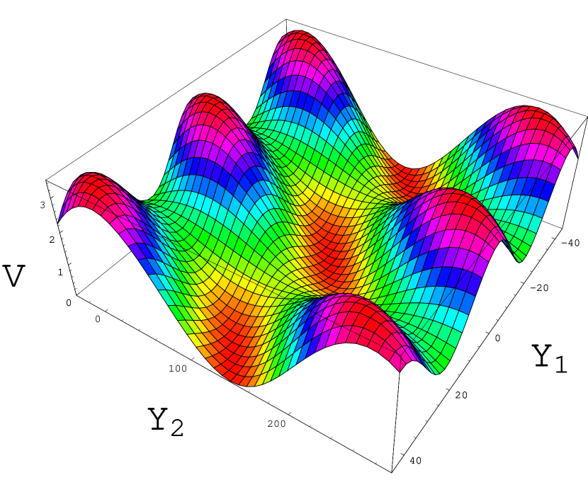
Figure 1: The potential as a function of the axion variables $Y_{1}$, $Y_{2}$ at the minimum of the radial variables $X_{1},X_{2}$, , in units $10^{{-15}}$ of the Planck density.

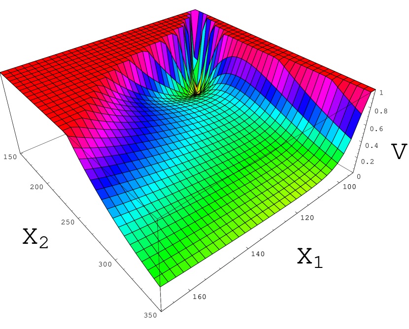
Figure 2: The potential as a function of the radial variables $X_{1}$, $X_{2}$ at the minimum of the angular variables $Y_{1},Y_{2}$, in units $10^{{-14}}$ of the Planck density.

With these choices of the parameters the minimum described above is located at

$$X_{1}=98.75839\qquad X_{2}=171.06117\qquad Y_{1}=0\qquad Y_{2}=129\,,$$ (33)

corresponding to a volume $R=99$ in string units, which is large enough to trust the effective field theory treatment we use. The parameter $D$ is tuned so that the potential vanishes at this minimum.

It is very difficult to plot the potential since it is a function of 4 variables. Here we will only show the behavior of this potential as a function of the axion variables $Y_{1}$, $Y_{2}$ at the minimum of the radial variables $X_{1},X_{2}$, and the potential as a function of the radial variables $X_{1}$, $X_{2}$ at the minimum of the angular variables $Y_{1},Y_{2}$. Figures 1 and 2 illustrate the behavior of the potential near the minimum (33).

We have checked that the eigenvalues of the Hessian (mass²) matrix are all positive, verifying that it is indeed a local minimum. The value of the masses for the moduli at this minimum turn out to be of order $10^{-6}-10^{-7}$ in Planck units.

Inflation occurs near the saddle point located at

$$X_{1}=108.96194\qquad X_{2}=217.68875\qquad Y_{1}=20\qquad Y_{2}=129\,.$$ (34)

At this point the mass matrix has three positive eigenvalues and one negative one in the direction of $(\delta X_{1},\delta X_{2},\delta Y_{1},\delta Y_{2})=(0,0,-0.6546,0.7560)$, corresponding to a purely axion direction. This is the initial direction of the slow roll away from the saddle point towards the nontrivial minimum described above.

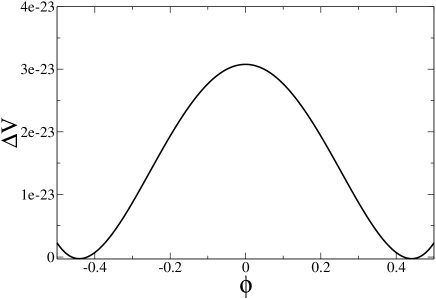
Figure 3: A cross section of the change in the potential near the saddle point, along the tangent to the initial unstable direction, in units of the Planck density.

The value of the effective potential at the saddle point is $V\sim 3.35\times 10^{{-16}}=M^{4}$ in Planck units, so that the scale of inflation is $M=3.25\times 10^{14}$ GeV. This is a rather small scale. The ratio of tensor to scalar perturbations in this scenario is very small, $r\ll 1$, so the gravitational waves produced in this scenario will be very hard to observe [37]. We plot the shape of the potential along the initial unstable direction, $(Y_{1},Y_{2})=(-0.6546,0.7560)\phi$ in figure 3. (The zero of the $y$-axis is not the true minimum of the potential since the real inflaton trajectory curves away from the initial tangent to the trajectory.)

To find the slow roll parameter $\eta$ at the saddle point (recall that $\epsilon=0$ automatically at a saddle point), as well as to compute the inflationary trajectories, we must also specify the kinetic terms for the fields. The general supergravity expression is given in terms of derivatives with respect to the Kähler potential,

$${\cal L}_{\rm kin}={\partial^{2}K\over\partial\phi_{i}^{*}\partial\phi_{j}}\,\partial_{\mu}\phi_{i}^{*}\partial^{\mu}\phi_{j}$$ (35)

Explicitly, we find

$${\cal L}_{\rm kin}\ = \ \frac{3}{8\left(X_{1}^{3/2}-X_{2}^{3/2}\right)^{2}}\left(\frac{2X_{1}^{3/2}+X_{2}^{3/2}}{\sqrt{X_{1}}}\ \left(\partial X_{1}^{2}+\partial Y_{1}^{2}\right)\ \right.$$

$$- 6\sqrt{X_{1}X_{2}}\,\left(\partial X_{1}\partial X_{2}+\partial Y_{1}\partial Y_{2}\right)+\left.\frac{X_{1}^{3/2}+2X_{2}^{3/2}}{\sqrt{X_{2}}}\,(\partial X_{2}^{2}+\partial Y_{2}^{2})\right)$$ (36)

The noncanonical kinetic terms require the use of the generalized definitions of the slow-roll parameters defined earlier. Alternatively, because the initial roll is purely in the $(Y_{1},Y_{2})$ plane we can instead choose to diagonalize the kinetic terms for the $Y_{i}$ fields in the approximation that the $X_{i}$’s are constants. This diagonalization is straightforward but cumbersome, and leads to the value

$$\eta=-0.01$$ (37)

at the saddle point. As we will discuss below, this leads to $n_{s}\approx 0.95$ and a long period of inflation, 980 $e$-foldings after the end of eternal inflation.

5 Normalization of spectrum and scale of inflation

We have computed the power spectrum for the model under consideration by first numerically evolving the full set of field equations, which can be efficiently written in the form

$${d\phi_{i}\over dN} = {1\over H}{\dot{\phi}_{i}}(\pi_{i})$$

$${d\pi_{i}\over dN} = -3\pi_{i}-{1\over H}{\partial\over\partial\phi_{i}}\left(V(\phi_{i})-{\cal L}_{\rm kin}\right)$$ (38)

where $N$ is the number of $e$-foldings starting from the beginning of inflation, $\pi_{i}=\partial{\cal L}_{\rm kin}/\partial\dot{\phi}_{i}$ are the canonical momenta, and the time derivatives ${\dot{\phi}_{i}}$ are regarded as functions of $\pi_{i}$, which can conveniently be solved for using symbolic manipulation. (This procedure alleviates the need for computing Christoffel symbols in field space, or explicitly diagonalizing the kinetic term. However we have also checked our results by directly integrating the second order equations for $X_{i},Y_{i}$ in Mathematica.) We use initial conditions where the field starts from rest along the unstable direction, close enough to the saddle point to give more than 60 e-foldings of inflation. In fact our starting point corresponds to the boundary of the eternally inflating region around the saddle point where the field is dominated by quantum fluctuations [38] . An example of the inflationary trajectories for all the fields is shown in figures 5-5.

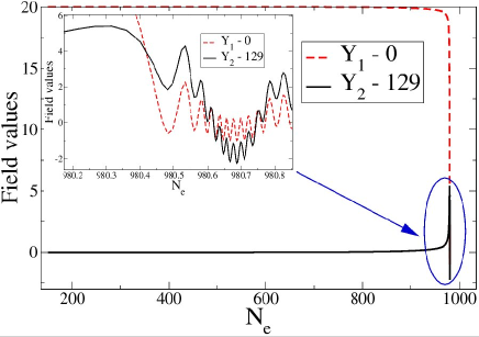
Figure 4: Evolution of the axionic fields $Y_{1},Y_{2}$ during inflation. Inset shows oscillations around the minimum at the end of inflation.

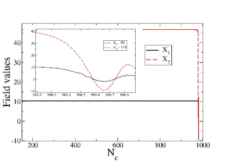
Figure 5: Evolution of the $X_{1},X_{2}$ directions during the inflationary period. Note that even though the potential at the minimum is only protected by a small barrier, our numerical evolutions shows that the fields do relax to this minimum evading a potential overshooting problem.

To compute the spectrum of adiabatic scalar density perturbations, we use the effective one-field approximation, namely that the power is given by

$$P(k)={1\over 50\pi^{2}}{H^{4}\over{\cal L}_{\rm kin}}$$ (39)

evaluated at horizon crossing, $k/a=H$. Equivalently, we can parametrize $P$ as a function of the number of $e$-foldings of inflation.

If we assume that the reheat temperature is of the same order as the scale of inflation, $T_{r}\sim M=3.25\times 10^{14}$ GeV, the number of $e$-foldings of inflation since horizon crossing is

$$N_{e}=53+\ln(M/10^{13}{\rm\ GeV})\approx 56.5$$ (40)

and the COBE normalization scale is at $\Delta N=N_{e}-\ln(k_{0}/(aH_{0}))=N_{e}-\ln(7.5)=N_{e}-2\sim 55$ $e$-foldings before the end of inflation. If $T_{r}<M$, then $N_{e}$ is reduced by the amount $\frac{1}{3}\ln(M/T_{r})$. For example, one might like to satisfy the gravitino bound $T_{r}<10^{10}$ GeV, which decreases $N_{e}$ to 53. The running of the spectral index (which will be studied in the next section) is sufficiently small that this changes the value of $n_{s}$ only by $-0.003$, thus our results do not depend sensitively on assumptions about the reheating temperature.

Our numerical analysis shows that the amplitude of density perturbations for the parameters given above does satisfy the COBE normalization of the power spectrum,

$$P(k_{0})=4\times 10^{-10}$$ (41)

at the COBE normalization scale.

6 Power spectrum, dependence on $W_{0}$, and anthropic considerations

The choice of the parameters leading to $P(k_{0})=4\times 10^{-10}$ is not unique. First of all, just as in the Racetrack scenario [12], there is a rescaling of parameters

$$(a,b)\to\lambda^{-1}\,(a,b),\quad\left(A,B,W_{0},D^{1/2}\right)\to\lambda^{3/2}\left(A,B,W_{0},D^{{1/2}}\right),\quad\left(X_{i},Y_{i}\right)\to\lambda\ \left(X_{i},Y_{i}\right)$$ (42)

This transformation does not alter inflationary dynamics or the height of the potential; it rescales the fields, but leaves the slow-roll parameters and the amplitude of density perturbations invariant. If a set of parameters gives rise to slow-roll inflation in a region of field space, the transformed parameters will also yield inflation with the same spectrum of density fluctuations, in the transformed region of field space.

A less trivial change occurs if we keep $a,b,X_{i},Y_{i}$ invariant and rescale $W_{0},A,B$ by $\mu^{-3/2}$ each and $D$ by $\mu^{-3}$. This transformation rescales the potential $V$ and the amplitude of density perturbations $P$ as $\mu^{3}$ without altering the values of the fields, the slow roll parameters, or the total duration of inflation.

It would be interesting to compare different sets of parameters related to each other by the $\mu$-transformation and find which of these parameters are more probable in the stringy landscape, which ones lead to the greater volume for the inflationary universe and more efficient reheating, etc. This would allow us to determine the most probable amplitude of density perturbations in this class of theories, see e.g. [41] for a discussion of closely related issues. This is a complicated problem which goes beyond the scope of the present investigation. We still do not know what is the proper choice for the probability measure in eternal inflation. In addition, it is not obvious whether a simultaneous scaling of several different parameters which have different origin can be easily achieved within the full string theory landscape.

Therefore we may instead pursue a more modest goal and study what happens when we change just one of the parameters, e.g., $W_{0}$. Let us recall the arguments concerning the distribution of flux vacua in string theory with a given value of $W_{0}$, [42], [43]. This distribution is believed to be uniform near zero. This means that if one wants $|W_{0}|\leq\epsilon$, the fraction of flux vacua that may provide this value is of the order $\epsilon^{2}$. Keeping in mind an enormously large number of flux vacua we deduce that any value of $W_{0}$ which we may need for cosmology is available, at least in principle, in some explicit constructions, in particular in the “better racetrack” model. To obtain the particular value which we need would require an intensive numerical search, by varying sets of stabilizing fluxes, and this is not guaranteed to be a computable problem in a reasonable amount of time [44]. It is therefore satisfying to know that at least in principle, the value of $W_{0}$ which we need in our model for cosmology is possible. Particularly, we may relax the restriction to the 2-parameter model defined in eq. (17) and engage all 272 complex structure moduli of the full model, which admits a huge number of possible fluxes. In this way we expect that eventually any required value of $W_{0}$ can be achieved constructively.

Since inflation in our scenario requires fine tuning, it is not surprising that a change of $W_{0}$ by several percent can spoil inflation. We have found, for example, that when one decreases $W_{0}$ from $5.227\times 10^{-6}$ to $5.147\times 10^{-6}$, i.e. by 1.5%, the height of the saddle point and the amplitude of perturbations change insignificantly, while $n_{s}$ decreases to $0.92$, which is at the verge of being ruled out by observations.

We have evaluated the scalar spectral index, $n_{s}=d\ln P/d\ln k$ at two different points along the inflationary trajectory: at the beginning, when the fields are near the saddle point, and at 50 $e$-foldings before the end of inflation, near the COBE normalization point. We carried this out for a range of $W_{0}$ values around our fiducial value $W_{0}=5.227\times 10^{-6}$, going up to the critical value $W_{c}=5.267\times 10^{-6}$, beyond which the saddle point becomes a local minimum. The results are shown in figure 7.

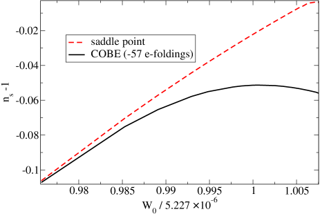
Figure 6: Spectral index at the saddle point and at the COBE scale, as a function of $W_{0}$ divided by its optimal value, with other parameters (except $D$) held fixed.

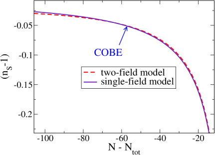
Figure 7: Spectral index as a function of the number of $e$-foldings of inflation (minus the total number of $e$-foldings), for the original racetrack model, and the two-Kähler modulus model of this paper.

Evaluating the spectral index at $55$ $e$-foldings before the end of inflation gives the spectral properties relevant for the CMB. Figure 7 shows that for $W_{0}=5.227\times 10^{-6}$ the spectral index reaches its largest value

$$n_{s}\approx 0.95$$ (43)

This is the same value which we found in the original racetrack model. The figure shows that $W_{0}$ has to be tuned at the level of a percent to keep the spectral index from decreasing into a range of phenomenologically disfavored values. The comparison between the model of this paper and the original single-Kähler modulus racetrack model is shown in figure 7, where we chose the endpoint of inflation to coincide for the two models, for ease of comparison. The figure plots the spectral index as a function the number of $e$-foldings, minus the total number of $e$-foldings, showing that the spectral properties of the two models are remarkably similar.

During most of inflation, the parameter $n_{s}$ remains nearly constant, at its value near the saddle point, shown in figure (7). Only during the latter part of its evolution does it move toward the smaller values which apply at horizon crossing. Since $\ln k\sim N$ during inflation, the power grows in the past like $P\sim e^{(n_{s}-1)N}$ to some approximation, where $n_{s}$ is evaluated at the saddle point. Knowing that $P(k_{0})=4\times 10^{-10}$ at the COBE point, we can thus roughly estimate the number of $e$-foldings $N_{b}$ from the end of the stage of eternal inflation, where $P=O(1)$, to the COBE point, where $P(k_{0})\sim 4\times 10^{-10}$:

$$N_{b}\sim{\ln(4\times 10^{-10})\over n_{s}-1}={C\over 1-n_{s}}\ ,$$ (44)

with $C\approx 20$. In the model with $W_{0}=5.227\times 10^{-6}$ one has $1-n_{s}\approx 0.022$ during the main part of inflation (much earlier than horizon crossing), which gives $N_{b}\approx 980$, in reasonable agreement with the actual value of 920 obtained numerically. (Note, however, that even though $n_{s}=0.98$ near the saddle point, its value at the COBE scale is $n_{s}=0.95$.). On the other hand, eq. (44) suggests that there will be a smaller number of $e$-foldings as we decrease the value of $n_{s}$. In fact, we have proved explicitly that this is indeed what happens in our model. Solving the equations of motion numerically we found that the number of $e$-folds after eternal inflation for the case with $n_{s}=0.92$ gives us $300$ $e$-folds instead of the $920$ of the $n_{s}=0.95$ case.

This means that the total volume of the universe after eternal inflation grows additionally by the factor of

$$e^{3N_{b}}\sim\exp\left({3C\over 1-n_{s}}\right).$$ (45)

One could arrive at a similar conclusion by investigating the total growth of the universe for inflation which begins when the field was at a given distance from the saddle point.

The meaning of this result is very simple: The small value of $1-n_{s}$ correspond to small values of the slow-roll parameters. One may argue that in this case eternal inflation near the saddle point becomes more efficient (“longer eternity”). In addition to it, the normal inflationary regime becomes longer, the growth of the volume of the universe is proportional to $\exp\left({3C\over 1-n_{s}}\right)$, and therefore the total volume of the universe will be dominated by the regions with the smallest possible values of $1-n_{s}$.

This argument has a following interesting implication, which seems quite plausible: If one assumes that the probability to live in a given part of the universe is proportional to its volume, this assumption singles out those parameters which lead to $n_{s}$ as close to 1 as possible. In this sense, one may argue that the value $W_{0}=5.227\times 10^{-6}$, which gives the largest value of $n_{s}$ in our model (all other parameters being fixed), is determined not by fine-tuning but by anthropic considerations: The parts of the universe with a flat spectrum of perturbations tend to have larger volume; the flatter the better.

7 Discussion

We have seen that the superpotential and Kähler potential which have been computed for compactifications to four dimensions on the orbifolded Calabi-Yau manifold, ${\rm I\kern-1.79993ptP}^{4}_{[1,1,1,6,9]}$, is rich enough to allow inflationary regimes to occur. These inflationary regimes resemble those of the original racetrack scenario inasmuch as they correspond to regions where $|\eta|$ is arranged to be small at a saddle point which lies between two degenerate minima.

In the KKLT model, with the superpotential containing only one exponent for the volume modulus, one could not have inflation without adding moving branes. In our original racetrack inflation scenario [12] we were able to find the first working inflationary model without adding any new branes to the KKLT vacuum stabilization scenario. In the present work we have made a new step and achieved inflation in a theory with two moduli fields, without introducing the standard racetrack potentials with two exponential terms for each of them. This suggests that by increasing the number of moduli fields, inflation may be easier to achieve. Actually, in Ref. [14] inflation is generically achieved in models with more than two Kähler moduli, but the inflaton in those models is the real part of a Kähler modulus rather than its axionic component. A similar observation was made in Ref. [45] in a different context.

The properties of the resulting density fluctuations in our model can be computed in the usual way in terms of the slow-roll parameters, leading to inflationary phenomenology which resembles in many ways that of the original racetrack inflation model. Depending on the choice of parameters for the improved racetrack, one can obtain spectra with different values of the spectral index $n_{s}$. We find it interesting that the volume of the universe becomes exponentially larger for the models with the smallest deviation of $n_{s}$ from unity. For the full range of inflationary parameters that we were able to find, the largest value of $n_{s}$, corresponding to the largest volume of the universe, is $n_{s}\approx 0.95$, which is in a good agreement with the latest observational data [36].

Finally, we would like to comment on the non-Gaussianity of the metric perturbations in our model. As should be clear from the discussion above, the model we are presenting can be recast as a single field inflation, once the trajectory in field space is obtained numerically. Based on this realization one would expect the non-Gaussianity in our model to be very small, and we checked numerically that this is indeed the case.

Note Added

This paper was completed shortly before the WMAP third year data release, and our results (including the prediction $n_{s}=0.95$) were reported by A.L. at the UK Cosmology Meeting, Newcastle University, March 14 2006.

References

- [1] G. R. Dvali and S. H. H. Tye, “Brane inflation,” Phys. Lett. B 450 (1999) 72 [arXiv:hep-ph/9812483].
- [2] C. P. Burgess, M. Majumdar, D. Nolte, F. Quevedo, G. Rajesh and R. J. Zhang, “The inflationary brane-antibrane universe,” JHEP 0107 (2001) 047 [arXiv:hep-th/0105204]. G. R. Dvali, Q. Shafi and S. Solganik, “D-brane inflation,” arXiv:hep-th/0105203.
- [3] J. Garcia-Bellido, R. Rabadan and F. Zamora, “Inflationary scenarios from branes at angles,” JHEP 0201, 036 (2002); N. Jones, H. Stoica and S. H. H. Tye, “Brane interaction as the origin of inflation,” JHEP 0207, 051 (2002); M. Gomez-Reino and I. Zavala, “Recombination of intersecting D-branes and cosmological inflation,” JHEP 0209, 020 (2002).
- [4] For reviews with more references see: F. Quevedo, Class. Quant. Grav. 19 (2002) 5721, [arXiv:hep-th/0210292]; A. Linde, “Prospects of inflation,” Phys. Scripta T117 (2005) 40 [arXiv:hep-th/0402051], C.P. Burgess, “Inflationary String Theory?,”Pramana 63 (2004) 1269 [arXiv:hep-th/0408037];
- [5] S. Kachru, R. Kallosh, A. Linde, J. Maldacena, L. McAllister and S. P. Trivedi, “Towards inflation in string theory,” JCAP 0310 (2003) 013 [arXiv:hep-th/0308055].
- [6] C. P. Burgess, J. M. Cline, H. Stoica and F. Quevedo, “Inflation in realistic D-brane models,” JHEP 0409 (2004) 033 [arXiv:hep-th/0403119].
- [7] J. M. Cline and H. Stoica, “Multibrane inflation and dynamical flattening of the inflaton potential,” Phys. Rev. D 72, 126004 (2005) [arXiv:hep-th/0508029].
- [8] J. P. Hsu, R. Kallosh and S. Prokushkin, “On brane inflation with volume stabilization,” JCAP 0312 (2003) 009 [arXiv:hep-th/0311077]; F. Koyama, Y. Tachikawa and T. Watari, “Supergravity analysis of hybrid inflation model from D3-D7 system”, [arXiv:hep-th/0311191]; H. Firouzjahi and S. H. H. Tye, “Closer towards inflation in string theory,” Phys. Lett. B 584 (2004) 147 [arXiv:hep-th/0312020]. J. P. Hsu and R. Kallosh, “Volume stabilization and the origin of the inflaton shift symmetry in string theory,” JHEP 0404 (2004) 042 [arXiv:hep-th/0402047];
- [9] E. Silverstein and D. Tong, “Scalar speed limits and cosmology: Acceleration from D-cceleration,” Phys. Rev. D 70 (2004) 103505 [arXiv:hep-th/0310221]. M. Alishahiha, E. Silverstein and D. Tong, “DBI in the sky,” Phys. Rev. D 70 (2004) 123505 [arXiv:hep-th/0404084]. X. g. Chen, “Inflation from warped space,” JHEP 0508 (2005) 045 [arXiv:hep-th/0501184]. X. G. Chen, “Running non-Gaussianities in DBI inflation,” arXiv:astro-ph/0507053.
- [10] D. Cremades, F. Quevedo and A. Sinha, “Warped tachyonic inflation in type IIB flux compactifications and the open-string completeness conjecture,” JHEP 0510 (2005) 106 [arXiv:hep-th/0505252].
- [11] C. P. Burgess, P. Martineau, F. Quevedo, G. Rajesh and R. J. Zhang, “Brane antibrane inflation in orbifold and orientifold models,” JHEP 0203 (2002) 052 [arXiv:hep-th/0111025].
- [12] J. J. Blanco-Pillado et al., “Racetrack inflation,” JHEP 0411 (2004) 063 [arXiv:hep-th/0406230].
- [13] Z. Lalak, G. G. Ross and S. Sarkar, “Racetrack inflation and assisted moduli stabilisation,” [arXiv:hep-th/0503178].
- [14] J. P. Conlon and F. Quevedo, “Kaehler moduli inflation,” JHEP 0601 (2006) 146 [arXiv:hep-th/0509012].
- [15] O. DeWolfe, S. Kachru and H. Verlinde, “The giant inflaton,” JHEP 0405 (2004) 017 [arXiv:hep-th/0403123]. N. Iizuka and S. P. Trivedi, “An inflationary model in string theory,” arXiv:hep-th/0403203.
- [16] N. V. Krasnikov, “On Supersymmetry Breaking In Superstring Theories,” Phys. Lett. B 193 (1987) 37. L.J. Dixon, ”Supersymmetry Breaking in String Theory”, in The Rice Meeting: Proceedings, B. Bonner and H. Miettinen eds., World Scientific (Singapore) 1990; T.R. Taylor, ”Dilaton, Gaugino Condensation and Supersymmetry Breaking”, Phys. Lett. B252 (1990) 59; B. de Carlos, J. A. Casas and C. Muñoz, “Supersymmetry breaking and determination of the unification gauge coupling constant in string theories,” Nucl. Phys. B 399 (1993) 623 [arXiv:hep-th/9204012].
- [17] S. Kachru, R. Kallosh, A. Linde and S. P. Trivedi, “de Sitter Vacua in String Theory,” Phys. Rev. D 68 (2003) 046005 [arXiv: hep-th/0301240].
- [18] F. Denef, M. R. Douglas and B. Florea, “Building a better racetrack,” JHEP 0406 (2004) 034 [arXiv:hep-th/0404257].
- [19] S. B. Giddings, S. Kachru and J. Polchinski, “Hierarchies from fluxes in string compactifications,” Phys. Rev. D66, 106006 (2002).
- [20] S. Sethi, C. Vafa and E. Witten, “Constraints on low-dimensional string compactifications,” Nucl. Phys. B 480 (1996) 213 [arXiv:hep-th/9606122]; K. Dasgupta, G. Rajesh and S. Sethi, “M theory, orientifolds and G-flux,” JHEP 9908 (1999) 023 [arXiv:hep-th/9908088].
- [21] E. Cremmer, S. Ferrara, C. Kounnas and D.V. Nanonpoulos, “Naturally vanishing cosmological constant in supergravity,” Phys. Lett. B133, 61 (1983); J. Ellis, A.B. Lahanas, D.V. Nanopoulos and K. Tamvakis, “No-scale Supersymmetric Standard Model,” Phys. Lett. B134, 429 (1984).
- [22] V. Balasubramanian, P. Berglund, J. P. Conlon and F. Quevedo, “Systematics of moduli stabilization in Calabi-Yau flux compactifications,” JHEP 0503 (2005) 007 [arXiv:hep-th/0502058]; J. P. Conlon, F. Quevedo and K. Suruliz, JHEP 0508 (2005) 007 [arXiv:hep-th/0505076]; J. P. Conlon, “The QCD axion and moduli stabilisation,” [arXiv:hep-th/0602233].
- [23] A. Westphal, “Eternal inflation with alpha’ corrections,” JCAP 0511 (2005) 003 [arXiv:hep-th/0507079]; B. Greene and A. Weltman, “An effect of alpha’ corrections on racetrack inflation,” arXiv:hep-th/0512135.
- [24] E. Witten, “Dimensional Reduction Of Superstring Models,” Phys. Lett. B 155 (1985) 151; C. P. Burgess, A. Font and F. Quevedo, “Low-Energy Effective Action For The Superstring,” Nucl. Phys. B 272 (1986) 661.
- [25] S. Kachru, J. Pearson and H. L. Verlinde, “Brane/flux annihilation and the string dual of a non-supersymmetric field theory,” JHEP 0206, 021 (2002) [arXiv:hep-th/0112197].
- [26] C. P. Burgess, R. Kallosh and F. Quevedo, “de Sitter string vacua from supersymmetric D-terms,” hep-th/0309187. A. Saltman and E. Silverstein, “The scaling of the no-scale potential and de Sitter model building,” JHEP 0411 (2004) 066 [arXiv:hep-th/0402135].
- [27] C. Escoda, M. Gomez-Reino and F. Quevedo, “Saltatory de Sitter string vacua,” JHEP 0311 (2003) 065 [arXiv:hep-th/0307160].
- [28] For more low-energy properties of supersymmetric product gauge groups see, for example, C. P. Burgess, A. de la Macorra, I. Maksymyk and F. Quevedo, “Supersymmetric models with product groups and field dependent gauge couplings,” JHEP 9809 (1998) 007 [arXiv:hep-th/9808087].
- [29] J. J. Blanco-Pillado, R. Kallosh and A. Linde, “Supersymmetry and stability of flux vacua,” arXiv:hep-th/0511042.
- [30] For reviews, see, A. Linde, Particle Physics and Inflationary Cosmology, Harwood Academic Publishers (1990) [arXiv:hep-th/0503203]; E. W. Kolb and M. S. Turner, The Early Universe, Addison-Wesley (1990); A. R. Liddle and D. H. Lyth, Cosmological Inflation and Large-Scale Structure, Cambridge University Press (2000).
- [31] See for example R. Kallosh and S. Prokushkin, “Supercosmology,” arXiv:hep-th/0403060; C.P. Burgess, P. Grenier and D. Hoover, JCAP 0403 (2004) 008, [arXiv:hep-ph/0308252].
- [32] P. Candelas, A. Font, S. Katz and D. R. Morrison, “Mirror symmetry for two parameter models. 2,” Nucl. Phys. B 429, 626 (1994) [arXiv:hep-th/9403187].
- [33] A. Giryavets, S. Kachru, P. K. Tripathy and S. P. Trivedi, “Flux compactifications on Calabi-Yau threefolds,” JHEP 0404, 003 (2004) [arXiv:hep-th/0312104].
- [34] S. Gukov, C. Vafa and E. Witten, “CFTs from Calabi-Yau Fourfolds,” Nucl. Phys. B584, 69 (2000).
- [35] K. Freese, J. A. Frieman and A. V. Olinto, “Natural Inflation With Pseudo - Nambu-Goldstone Bosons,” Phys. Rev. Lett. 65, 3233 (1990); F. C. Adams, J. R. Bond, K. Freese, J. A. Frieman and A. V. Olinto, “Natural inflation: Particle physics models, power law spectra for large scale structure, and constraints from COBE,” Phys. Rev. D 47 (1993) 426 [arXiv:hep-ph/9207245].
- [36] C. J. MacTavish et al., “Cosmological parameters from the 2003 flight of BOOMERANG,” arXiv:astro-ph/0507503.
- [37] G. Efstathiou and S. Chongchitnan, “The Search For Primordial Tensor Modes,” arXiv:astro-ph/0603118.
- [38] A. D. Linde, “Monopoles as big as a universe,” Phys. Lett. B 327, 208 (1994) [arXiv:astro-ph/9402031]; A. Vilenkin, “Topological inflation,” Phys. Rev. Lett. 72, 3137 (1994) [arXiv:hep-th/9402085].
- [39] R. Brustein and P. J. Steinhardt, “Challenges for superstring cosmology,” Phys. Lett. B 302 (1993) 196 [arXiv:hep-th/9212049].
- [40] W. Buchmuller, K. Hamaguchi, O. Lebedev and M. Ratz, “Maximal temperature in flux compactifications,” JCAP 0501 (2005) 004 [arXiv:hep-th/0411109].
- [41] A. D. Linde, D. A. Linde and A. Mezhlumian, “From the Big Bang theory to the theory of a stationary universe,” Phys. Rev. D 49, 1783 (1994) [arXiv:gr-qc/9306035]; J. Garcia-Bellido, A. D. Linde and D. A. Linde, “Fluctuations of the gravitational constant in the inflationary Brans-Dicke cosmology,” Phys. Rev. D 50, 730 (1994) [arXiv:astro-ph/9312039]; A. Vilenkin, “The Birth Of Inflationary Universes,” Phys. Rev. D 27 (1983) 2848; J. Garcia-Bellido and A. D. Linde, “Stationarity of inflation and predictions of quantum cosmology,” Phys. Rev. D 51, 429 (1995) [arXiv:hep-th/9408023]; M. Tegmark and M. J. Rees, “Why is the CMB fluctuation level ?,” Astrophys. J. 499, 526 (1998) [arXiv:astro-ph/9709058]. B. Feldstein, L. J. Hall and T. Watari, “Density perturbations and the cosmological constant from inflationary landscapes,” Phys. Rev. D 72, 123506 (2005) [arXiv:hep-th/0506235]; J. Garriga and A. Vilenkin, “Anthropic prediction for Lambda and the Q catastrophe,” arXiv:hep-th/0508005; J. Garriga, D. Schwartz-Perlov, A. Vilenkin and S. Winitzki, “Probabilities in the inflationary multiverse,” JCAP 0601, 017 (2006) [arXiv:hep-th/0509184]; A. Linde and V. Mukhanov, “The curvaton web,” arXiv:astro-ph/0511736; M. Tegmark, A. Aguirre, M. Rees and F. Wilczek, “Dimensionless constants, cosmology and other dark matters,” Phys. Rev. D 73, 023505 (2006) [arXiv:astro-ph/0511774]. L. J. Hall, T. Watari and T. T. Yanagida, “Taming the runaway problem of inflationary landscapes,” arXiv:hep-th/0601028; D. H. Lyth, “Non-gaussianity and cosmic uncertainty in curvaton-type models,” arXiv:astro-ph/0602285.
- [42] S. Kachru, private communication, 2003.
- [43] M. R. Douglas, “Statistical analysis of the supersymmetry breaking scale,” arXiv:hep-th/0405279.
- [44] F. Denef and M. R. Douglas, “Computational complexity of the landscape. I,” arXiv:hep-th/0602072.
- [45] S. Dimopoulos, S. Kachru, J. McGreevy and J. G. Wacker, “N-flation,” arXiv:hep-th/0507205.
- [46] C. Y. Sun and D. H. Zhang, “The non-Gaussianity of racetrack inflation models,” arXiv:astro-ph/0604298.