SINP-TNP/06-09

Quasinormal modes for tensor and vector type perturbation of

Gauss Bonnet black hole using third order WKB approach

Abstract

We obtain the quasinormal modes for tensor perturbations of Gauss-Bonnet (GB) black holes in $d=5,7,8$ dimensions and vector perturbations in $d=5,6,7$ and $8$ dimensions using third order WKB formalism. The tensor perturbation for black holes in $d=6$ is not considered because of the fact that it is unstable to tensor mode perturbations. In the case of uncharged GB black hole, for both tensor and vector perturbations, the real part of the QN frequency increases as the Gauss-Bonnet coupling ($\alpha^{\prime}$) increases. The imaginary part first decreases upto a certain value of $\alpha^{\prime}$ and then increases with $\alpha^{\prime}$ for both tensor and vector perturbations. For larger values of $\alpha^{\prime}$, the QN frequencies for vector perturbation differs slightly from the QN frequencies for tensorial one. It has also been shown that as $\alpha^{\prime}\to 0$, the quasinormal mode frequency for tensor and vector perturbation of the Schwarzschild black hole can be obtained. We have also calculated the quasinormal spectrum of the charged GB black hole for tensor perturbations. Here we have found that the real oscillation frequency increases, while the imaginary part of the frequency falls with the increase of the charge. We also show that the quasinormal frequencies for scalar field perturbations and the tensor gravitational perturbations do not match as was claimed in the literature. The difference in the result increases if we increase the GB coupling.

Keywords: Quasinormal modes, Gauss-Bonnet black holes, Vector and Tensor perturbations

PACS : 04.70.-s, 04.50.+h

1.  Introduction

Quasinormal Modes (QNMs) are of great relevance in discussing the perturbations of black holes [1, 2, 3, 4, 5, 6]. For a large class of black holes, the equations governing the perturbations can be cast into the Schrödinger like wave equation. For asymptotically flat space-times, the QNMs are solutions of the corresponding wave equation with complex frequencies which are purely ingoing at the horizon and purely outgoing at spatial infinity [1, 2]. QNMs associated with metric perturbations have been found to be a useful probe of the underlying space-time geometry [3, 5]. QN frequencies carry unique information about black hole parameters and are expected to be detected in future gravitational wave detectors [7]. In addition, it has also been shown that quasinormal modes in Anti-de Sitter space-time appear naturally in the description of the corresponding dual conformal field theories living on the boundary [8, 9]. In spite of their classical origin, it has also been suggested that QNMs might provide a glimpse into the quantum nature of the black hole [10, 11, 12, 13, 14, 15].

QNMs of black holes have been traditionally studied for the backgrounds which arise out of the Einstein’s theory of general relativity (see [1, 2] for a complete list of references). Recently there has been a renewed interest in black holes arising from higher curvature corrections to Einstein-Hilbert action, partly due to new developments in string theory [16, 17]. Low energy limits of string theories give rise to effective models of gravity in higher dimensions. These effective models of gravity involve higher powers of the Riemann curvature tensor in the action in addition to the usual Einstein-Hilbert term [18]. Among these higher powers of Riemann curvature, the Gauss-Bonnet combination is of special interest [19, 20, 21, 22, 23]. The Gauss-Bonnet black holes has also been discussed in the context of brane world models [24]. The entropy and related thermodynamic properties of GB black holes have been discussed in [25, 26, 27, 28, 29, 30]. Recently GB black holes have received attention in the context of possible production at the LHC [31].

Scalar QN frequencies of the Gauss-Bonnet black holes were first discussed long time ago [32], where the scalar modes of the uncharged GB black hole for a few values of the Gauss-Bonnet coupling were evaluated in $5$ and $6$ dimensions. Recently, in [33] the QNMs for scalar perturbations of neutral and charged Gauss-Bonnet black holes have been discussed. In a related work a detailed analysis of scalar perturbations in the background of Gauss-Bonnet, Gauss-Bonnet-de Sitter and Gauss-Bonnet-Anti-de Sitter black hole space-time were presented [34]. Using both numerical as well as a semi-analytic WKB approach it has been shown that the scalar field evolution is dependent on the cosmological constant and the GB coupling. The late time behaviors of the scalar fields were also discussed there.

In this paper we shall discuss the QNMs for tensor and vector perturbations of the neutral Gauss-Bonnet black hole using a semi-analytic WKB approach [35]. It was claimed in the literature [33] that the QN frequencies of the scalar field perturbations and the tensor perturbations would be the same even in the case of black holes arising in the Gauss-Bonnet gravity. We explicitly show that they do not give rise to the same QN frequency for GB black holes. We use the potential for tensor and vector mode perturbations of static spherically symmetric solutions of the Einstein equations with a Gauss-Bonnet term in dimensions $d>4$ as analyzed in [36, 37] respectively. Using the form of the potential in [36, 37] we obtain QN frequencies of the Gauss-Bonnet black holes for different multipole numbers $l$ and different values of the GB coupling. We have found that the quasinormal behavior for the tensor and vector perturbation is dependent on the GB coupling. We have also shown that the QN frequencies approach their Schwarzschild values when the GB coupling tends to zero. The new results obtained in this paper are as follows:
-The QN frequencies for vector and tensor perturbations of the GB black hole are obtained using the WKB method.
-We show that the quasinormal frequencies for scalar field perturbations and the tensor gravitational perturbations do not match as was claimed in the literature [33] and the difference in the result increases when the GB coupling is increased.
-It is shown that the Schwarzschild QN frequencies can be obtained from the values of QN frequencies of the Gauss-Bonnet black hole when the GB coupling goes to zero.

This paper is organized as follows: In Section 2 we shall briefly review the Gauss-Bonnet action and the tensor perturbation of the spherically symmetric Gauss-Bonnet space-time and will apply the third order WKB formula to obtain QN frequencies for tensor and vector perturbations of the Gauss-Bonnet black hole. Section 3 concludes the paper with some discussion of our results and an outlook.

2.  Tensor and vector perturbation of spherically symmetric Gauss-Bonnet space-time and the Gauss-Bonnet black hole

In space-time dimensions $d\geq 5$ the Einstein-Gauss-Bonnet action is given by

$$I=\frac{1}{16\pi G_{d}}\int d^{d}x\sqrt{-g}R+\alpha^{\prime}\int d^{d}x\sqrt{-g}(R_{\mu\nu\beta\gamma}R^{\mu\nu\beta\gamma}-4R_{\beta\gamma}R^{\beta\gamma}+R^{2}),$$ (2.1)

where $G_{d}$ is the $d$-dimensional Newton’s constant and the parameter $\alpha^{\prime}$ denotes the Gauss-Bonnet coupling. We will choose $G_{d}=1$ from now on and will consider only positive $\alpha^{\prime}$ which is consistent with the string expansion [20].

We consider the metric in space-time dimension $d$ [36]

$$ds^{2}=-f(r)dt^{2}+f^{-1}(r)dr^{2}+r^{2}\bar{g}_{ij}dy^{i}dy^{j}$$ (2.2)

where $\bar{g}_{ij}dy^{i}dy^{j}$ is the line element of the unit $(d-2)$-dimensional sphere. Here, the latin indices $i,j,k,..$ and a bar is used to denote tensors and operators in $S^{d-2}$[36]. Considering the tensor perturbations $g_{\mu\nu}\to g_{\mu\nu}+h_{\mu\nu}$, and using the following ansatz:

$$h_{ij}(t,r,y)=r^{2}\phi(r,t)\bar{h}_{ij}(y)\,\,\,\rm{and}\,\,\,\phi(r,t)=e^{\omega t}\chi(r),$$ (2.3)

one obtains the linearized Einstein-Gauss-Bonnet equations [36]

$$\delta G_{(1)\mu}~{}^{\nu}+\alpha^{\prime}\delta G_{(2)\mu}~{}^{\nu}=0$$ (2.4)

where

$$G_{(2)\mu}~{}^{\nu}=R_{\sigma\mu}^{~{}\beta\gamma}R_{\beta\gamma}^{~{}\sigma\nu}-2R_{\beta}^{~{}\sigma}R_{\sigma\mu}^{~{}\beta\nu}-2R_{\mu}^{~{}\sigma}R_{\sigma}^{~{}\nu}+RR_{\mu}^{~{}\nu}-\frac{1}{4}\delta_{\mu}^{\nu}(R_{\sigma\beta}^{~{}\gamma\delta}R_{\gamma\delta}^{~{}\sigma\beta}-4R_{\sigma}^{~{}\beta}R_{\beta}^{~{}\sigma}+R^{2})$$ (2.5)

From here on we will use subscript $T$ and $V$ to denote quantities relating to tensor and vector perturbations respectively. Now, introducing $\Phi(r)=\chi(r)K_{T}(r)$, Eqn. (2.4) reduces to a second order ordinary differential equation [36]:

$$-\frac{d^{2}\Phi}{dx^{2}}+V(r(x))\Phi=\omega^{2}\Phi$$ (2.6)

Where $x$ is the “tortoise coordinate” defined by $\frac{dx}{dr}=\frac{1}{f(r)}$, where $r=\infty$ corresponds to $x=\infty$ and the event horizon $r=r_{h}$ corresponds to $x=-\infty$. Now, $K_{T}(r)$ is defined as :

$$K_{T}(r)=r^{\frac{d-4}{2}}\sqrt{r^{2}~{}+~{}\alpha^{\prime}(d-4)\left[(d-5)(1-f(r))~{}-~{}r\frac{df}{dr}\right]}.$$ (2.7)

Now, the potential has the form [36]

$$V_{T}(r)=q_{T}(r)+\left(f\frac{d}{dr}ln(K_{T})\right)^{2}+f\frac{d}{dr}\left(f\frac{d}{dr}ln(K_{T})\right)$$ (2.8)

with $q_{T}(r)$ being given by:

$$q_{T}(r)=\left(\frac{f(2-\gamma)}{r^{2}}\right)\left(\frac{(1-\alpha^{\prime}f^{\prime\prime}(r))r^{2}+\alpha^{\prime}(d-5)[(d-6)(1-f(r))-2rf^{\prime}(r)]}{r^{2}+\alpha^{\prime}(d-4)[(d-5)(1-f(r))-rf^{\prime}(r)]}\right),$$ (2.9)

where $\gamma=-l(l+d-3)+2$ and $l=2,3,4,\cdots$ [38, 39]. It is important to mention that the results of Dotti and Gleiser readily reproduces the results of Einstein gravity in the $\alpha^{\prime}\to 0$ limit, which was studied by Ishibashi and Kodama [40, 41].

The vector perturbations of the Einstein-Gauss-Bonnet spacetime was discussed in [37]. The method used there is different from the computations carried out for the tensor perturbations. Without going into the details of the techniques used in [37], we mention here the potential for vector perturbation:

$$V_{V}(r)=q_{V}(r)+\frac{1}{K_{V}(r)}\left[\left(\frac{d^{2}K_{V}}{dr^{2}}\right)f^{2}+\left(\frac{dK_{V}}{dr}\right)f\frac{df}{dr}\right]$$ (2.10)

where

$$K_{V}(r)=\left[r^{(d-2)}+\alpha^{\prime}(d-4)r^{2}\frac{\partial}{\partial r}(r^{(d-5)}(1-f))\right]$$ (2.11)

and

$$q_{V}(r)=\frac{f[(l(l+d-3)-1)-(d-3)]H}{r^{2}},\,\,l=1,2,3...$$ (2.12)

where,

$$H=\frac{\alpha^{\prime 2}(d-2)(d-4)^{2}(d-5)(d-3)\psi^{2}+2\alpha^{\prime}(d-2)(d-4)(d-5)\psi+4(d-4)\Lambda\alpha^{\prime}+2(d-2)}{2(d-2)((d-3)(d-4)\psi\alpha^{\prime}+1)^{2}}$$

Here $\psi(r)$ is a solution of

$$\frac{(d-2)(d-3)(d-4)}{4}\psi^{2}+\frac{(d-2)}{2\alpha^{\prime}}\psi-\frac{\Lambda}{(d-1)\alpha^{\prime}}=\frac{M}{\alpha^{\prime}r^{(d-1)}}$$ (2.13)

Where $\Lambda$ is the cosmological constant. In what follows, we shall take $\Lambda=0$.

2a. Uncharged Gauss-Bonnet Black Hole

The metric for spherically symmetric asymptotically flat Gauss-Bonnet black hole solution of mass $M$ is given by Eqn. (2.2), where $f(r)$ has the form [20]

$$f(r)=1+\frac{r^{2}}{2\alpha}-\frac{r^{2}}{2\alpha}\sqrt{1+\frac{8\alpha M}{r^{d-1}}},$$ (2.14)

where,

$$\alpha=16\pi G_{d}(d-3)(d-4)\alpha^{\prime}.$$ (2.15)

For $\alpha^{\prime}>0$, this black hole admits only a single horizon [20]. The horizon $r=r_{h}$ is determined by the real positive solution of the equation

$$r_{h}^{d-3}+\alpha r_{h}^{d-5}=2M.$$ (2.16)

For most spacetime geometries, the wave equation governing the QNMs is not exactly solvable. Various numerical schemes have been used in the literature to find the QN frequencies, which include direct integration of the wave equation in the frequency domain [42], Pöschl-Teller approximation [43], WKB method [44, 45, 35, 46], phase integral method [47, 48] and continued fraction method [49]. We will use the WKB method in this paper.

The formula for QN frequencies using third order WKB approach is given by [44, 35]

$$\omega^{2}=[V_{0}+(-2V_{0}^{\prime\prime})^{1/2}\tilde{\Lambda}(n)]-i(n+\frac{1}{2})(-2V_{0}^{\prime\prime})^{1/2}[1+\tilde{\Omega}(n)].$$ (2.17)

where, $\tilde{\Lambda}=\Lambda/i$ and $\tilde{\Omega}=\Omega/(n+\frac{1}{2})$ and $\Lambda$ and $\Omega$ are given by

$$\Lambda(n) = \frac{i}{(-2V^{\prime\prime}_{0})^{1/2}}\left[\frac{1}{8}\left(\frac{V^{(4)}_{0}}{V^{\prime\prime}_{0}}\right)\left(\frac{1}{4}+\nu^{2}\right)-\frac{1}{288}\left(\frac{V^{(3)}_{0}}{V^{\prime\prime}_{0}}\right)^{2}(7+60\nu^{2})\right],$$

$$\Omega(n) = \frac{(n+\frac{1}{2})}{(-2V^{\prime\prime}_{0})^{1/2}}\bigg{[}\frac{5}{6912}\left(\frac{V^{(3)}_{0}}{V^{\prime\prime}_{0}}\right)^{4}(77+188\nu^{2})$$ (2.18)

$$-\frac{1}{384}\left(\frac{V^{(3)^{2}}_{0}V^{(4)}_{0}}{V^{\prime\prime^{3}}_{0}}\right)(51+100\nu^{2})+\frac{1}{2304}\left(\frac{V^{(4)}_{0}}{V^{\prime\prime}_{0}}\right)^{2}(67+68\nu^{2})$$

$$+\frac{1}{288}\left(\frac{V^{(3)}_{0}V^{(5)}_{0}}{V^{\prime\prime^{2}}_{0}}\right)(19+28\nu^{2})-\frac{1}{288}\left(\frac{V^{(6)}_{0}}{V^{\prime\prime}_{0}}\right)(5+4\nu^{2})\bigg{]}.$$

Where, $V^{(n)}_{0}=(d^{n}V/dx^{n})_{x=x_{0}}$ and $\nu=n+1/2$.

It may be mentioned here that the accuracy of the WKB method depends on the multipole number $l$ and the overtone number $n$. It has been shown [50] that the WKB approach is a good one for $l>n$, i.e. the numerical and the WKB results are in good agreement if $l>n$, but the WKB approach is not so good if $l=n$ and not at all applicable for $l<n$.

Now, using Eqns. (2.17), (2.18) and Eqns. (2.8), (2.10) we numerically evaluate the QNMs of this black hole. In Tables 1-3 we present the quasinormal frequencies for the uncharged Gauss-Bonnet black hole for tensor perturbation, where the metric is given by Eqn. (2.2) with $f(r)$ being given by Eqn. (2.14) in $d=5,7\,\,\rm{and}\,\,8$ for $l=2,3\,\,\rm{and}\,\,4$. Here the black hole in $d=6$ is not considered because of the fact that it is unstable to tensor mode perturbations [36]. Note also that in $d=5$, the horizon is at $r_{h}=\sqrt{2-\alpha}$. Thus for $d=5$, black hole type solutions exist only for $\alpha<2$ and hence the corresponding entries in the table are kept empty. We have calculated the frequencies for fundamental overtone $(n=0)$, which will be dominating in a signal. We have set $M=1$ in our calculations.

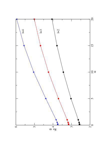
Figure 3: Re $\omega$ as a function of Gauss-Bonnet coupling $\alpha$ for $l=2,3,4$ and $n=0$ in $d=8$ for tensor perturbations.

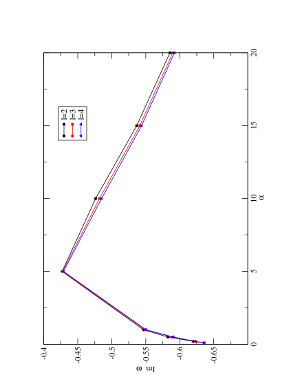
Figure 5: Im $\omega$ as a function of Gauss-Bonnet coupling $\alpha$ for $l=2,3,4$ and $n=0$ in $d=8$ for tensor perturbations.

The behavior of the real part of the quasinormal mode frequencies with the Gauss Bonnet coupling $\alpha$ in seven and eight dimensions respectively are shown in Figure 3 and 3. In Figure 5 and 5, we have plotted the behavior of imaginary part of the quasinormal frequency with the coupling $\alpha$ in $d=7\,\rm{and}\,8$ respectively. It is observed that the real part of the quasinormal mode frequency increases with $\alpha$, i.e the real oscillation frequency increases as the Gauss-Bonnet coupling increases. But the imaginary part shows a different kind of behavior, the damping decreases as $\alpha$ is increased from some lower values until some minimum value and then the damping increases as we go to larger values of $\alpha$.

In [33], scalar perturbations of the Gauss-Bonnet black hole were considered and it was shown that the quasinormal modes have greater oscillation frequency and greater damping rate at large $\alpha$. However, at moderate $\alpha$, the damping rate is decreasing until some minimum value and then begin to grow as a function of $\alpha$. It has been mentioned in [33] that the tensor type gravitational potential and the scalar field potential coincide as in the case of higher dimensional black holes in Einstein gravity as was established in [40]. But it was shown by Dotti and Gleiser [36] that the tensor perturbations of the Einstein-Gauss-Bonnet black hole is completely different from that of the tensor perturbations of black holes in Einstein gravity and as the Gauss-Bonnet coupling $\alpha$ goes to zero, the results of Einstein gravity can be recovered. We give a plot in fig. 1 to show how the potential for tensor gravitational perturbations and the scaler perturbation differ for a particular value of $\alpha$ and $l$.

 

Figure 1: Comparison between the potential for tensor gravitational perturbations and scalar field perturbations for Gauss-Bonnet black hole for $\alpha=1$ and $l=2$. The lower curve denotes the potential for tensor gravitational perturbations while the upper one denotes the same for scaler field perturbations.

Here we have used the potential for tensor perturbations obtained by Dotti and Gleiser and derived the QN frequencies for tensor perturbations of the Gauss-Bonnet black holes. The qualitative behavior of real and imaginary part of QN frequencies for tensor perturbations with $\alpha$ that we have obtained, is similar to that obtained in [33], where scalar perturbations were considered. If we compare our results with the results obtained in [33] for $d=7,\,\rm{and}\,\,l=2$, then we find that the real and imaginary parts of the QN frequency are different and the difference increases as $\alpha$ is increased. For example, the real and imaginary parts of our result differs from [33] by $0.5\%$ and $0.7\%$ respectively for $\alpha=0.1$, but the difference is $9\%$ and $1\%$ respectively for $\alpha=20$.

Here, we have used third order WKB approximation to find the quasinormal frequency of the Gauss-Bonnet black hole as we were unable to use sixth order corrections to this formula due to computational complcacies. However, there is not a very huge difference between third and sixth order result of QN frequencies for $l>n$ [46]. In the case for $l=0$, where the lowest overtone implies $l=n$, the WKB formula has a large amount of error when third order results are compared with the accurate numerical result for the Schwarzschild black hole, while the sixth order results almost matches with the numerical result [46]. But as we are considering tensor perturbations, where the lowest overtone implies $l>n$, we expect that the third order WKB treatment will be of good accuracy.

We have also verified that indeed the Schwarzschild QN frequency for tensorial perturbations can be obtained if $\alpha$ tends to zero. Now, to see that the numerical value of the QN frequency of the Gauss-Bonnet black hole approaches the value of the quasinormal mode frequency of the Schwarzschild black hole, we first consider six sample modes ($d=5,\,l=2,\,n=0$), found out from different small values of $\alpha$, $\alpha=1/100,1/200,1/300,1/400,1/500$ as considered in [33]. Then we find the quadratic fit and get

$$\omega=(1.06566-0.25305i)+(0.06285+0.05782i)\alpha+(0.16704-0.06213i)\alpha^{2}+O[\alpha^{3}]$$ (2.19)

So, we observe that the fit is approaching the fundamental ($n=0$) and $l=2$ quasinormal frequency for tensor type perturbation of the Schwarzschild black hole in five dimension, which is $1.0681-0.2529i$ [52]. It may be mentioned here that in [52], sixth order WKB correction formula was used to determine the quasinormal frequencies, but due to the complicacy of the potential here we were forced to use third order WKB correction formula. Therefore we expect that one can get more exact value of the frequency from the fit if sixth order WKB correction formula is used.

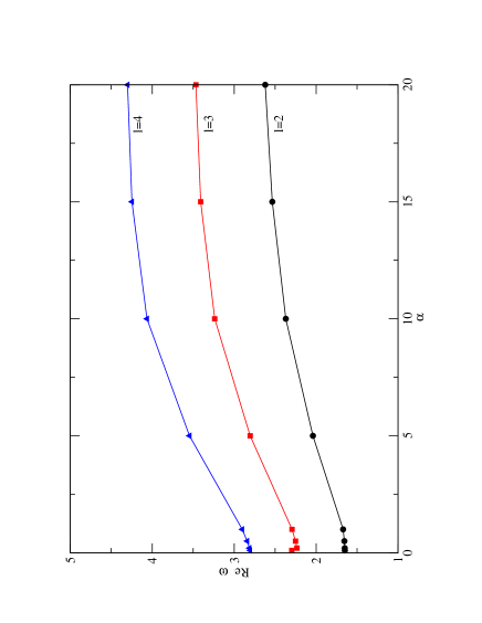
Figure 6: Re $\omega$ as a function of Gauss-Bonnet coupling $\alpha$ for $l=2,3,4$ and $n=0$ in $d=7$ for vector perturbations.

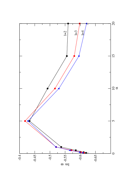
Figure 9: Im $\omega$ as a function of Gauss-Bonnet coupling $\alpha$ for $l=2,3,4$ and $n=0$ in $d=8$ for vector perturbations.

The numerical results for the quasinormal modes for vector perturbations are given in Tables 4-7. Here we have considered the values of $l=1,2,3$ and $4$ in $d=5,6,7$ and $8$ dimensions. As there is no problem of stability of the black hole in $d=6$ under vector perturbations like the tensor perturbation case, we consider $d=6$ also. But the problem with $d=6$ is that we are getting double peaks in the potential for larger values of $\alpha$. As that causes problem in the WKB analysis we left the corresponding entries in the tables blank. There is also some problem with the QN frequencies of $l=1$ in the case of vector perturbations. The nature of the dependence of QN frequencies for $l=1$ differ a little bit with those of $l=2,\,3\,\rm{and}\,4$. The probable cause for this might be due to the fact that we are using third order WKB approach to determine the QN frequencies. If sixth order treatment is used, we think that results from $l=1$ will be less erroneous. The plot for real and imaginary parts of the QN frequency in seven and eight dimensions are shown in fig. 6 - fig. 9 respectively.

Like the tensorial perturbations, here also we checked that Schwarzschild QN frequencies can be obtained from lower values of $\alpha$. For that we first consider five sample modes ($d=5,\,l=2,\,n=0$), found out from different small values of $\alpha$, $\alpha=1/100,1/200,1/300,1/400,1/500$. Then we find the quadratic fit and get

$$\omega=(0.80559-0.23545i)+(0.03376+0.005496i)\alpha+(0.00465+0.00729i)\alpha^{2}+O[\alpha^{3}]$$ (2.20)

We note that the fit is approaching the fundamental ($n=0$) and $l=2$ quasinormal frequency for vector type perturbation of the Schwarzschild black hole in five dimension, which is $0.8056-0.2355i$ [52]

$\alpha$	$\omega$
	d=5	d=7	d=8
0.1	1.07234-0.24737i	2.09158-0.51813i	2.57245-0.63574i
0.2	1.07949-0.24175i	2.09568-0.50563i	2.57391-0.61982i
0.5	1.10393-0.22500i	2.11523-0.47490i	2.58863-0.58251i
1.0	1.15641-0.19529i	2.16399-0.44120i	2.63419-0.54656i
5.0	-	2.64723-0.33309i	3.02722-0.42703i
10.0	-	3.31276-0.43274i	3.43874-0.47634i
15.0	-	3.84348-0.52104i	3.78370-0.53669i
20.0	-	4.23657-0.59334i	4.05205-0.58548i

Table 1: Quasinormal mode frequencies for tensor perturbation for $l=2$ in $d=5,7$ and $8$

$\alpha$	$\omega$
	d=5	d=7	d=8
0.1	1.42825-0.24648i	2.62080-0.51715i	3.15722-0.63605i
0.2	1.43818-0.24123i	2.62803-0.50632i	3.16206-0.62266i
0.5	1.47124-0.22497i	2.65471-0.47757i	3.18328-0.58829i
1.0	1.54074-0.19430i	2.71209-0.44140i	3.23448-0.54912i
5.0	-	3.33102-0.33905i	3.70504-0.42783i
10.0	-	4.19705-0.43708i	4.24267-0.48196i
15.0	-	4.87089-0.52488i	4.67515-0.54131i
20.0	-	5.36533-0.59728i	5.00776-0.58973i

Table 2: Quasinormal mode frequencies for tensor perturbation for $l=3$ in $d=5,7$ and $8$

$\alpha$	$\omega$
	d=5	d=7	d=8
0.1	1.78374-0.24604i	3.14573-0.51602i	3.73477-0.63489i
0.2	1.79630-0.24094i	3.15560-0.50603i	3.74238-0.62289i
0.5	1.83780-0.22488i	3.18919-0.47854i	3.77012-0.59069i
1.0	1.92439-0.19367i	3.25649-0.44120i	3.82896-0.55030i
5.0	-	4.01271-0.34219i	4.38417-0.42912i
10.0	-	5.07277-0.43935i	5.04128-0.48505i
15.0	-	5.88797-0.52690i	5.55942-0.54389i
20.0	-	6.48321-0.59934i	5.95548-0.59212i

Table 3: Quasinormal mode frequencies for tensor perturbation for $l=4$ in $d=5,7$ and $8$

      

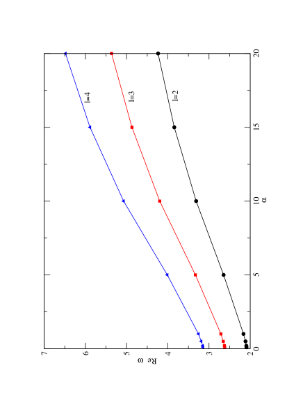
Figure 2: Re $\omega$ as a function of Gauss-Bonnet coupling $\alpha$ for $l=2,3,4$ and $n=0$ in $d=7$ for tensor perturbations.

          

      

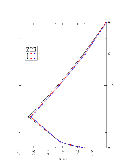
Figure 4: Im $\omega$ as a function of Gauss-Bonnet coupling $\alpha$ for $l=2,3,4$ and $n=0$ in $d=7$ for tensor perturbations.

          

$\alpha$	$\omega$
	d=5	d=6	d=7	d=8
0.1	0.38852-0.23491i	0.71811-0.37339i	1.08031-0.50041i	1.46373-0.61715i
0.2	0.38845-0.23310i	0.71772-0.37044i	1.07951-0.49660i	1.46250-0.61271i
0.5	0.38801-0.22691i	0.71640-0.36036i	1.07711-0.48362i	1.45897-0.59754i
1.0	0.38612-0.21348i	0.71389-0.33903i	1.07361-0.45689i	1.45410-0.56680i
5.0	-	0.95379-0.07595i	1.33952-0.45084i	1.66619-0.49783i
10.0	-	-	1.46092-0.36981i	1.79779-0.39821i
15.0	-	-	1.68586-0.47334i	1.94080-0.49012i
20.0	-	-	1.87237-0.54573i	2.07360-0.54533i

Table 4: Quasinormal mode frequencies for vector perturbation for $l=1$ in $d=5,6,7$ and $8$

$\alpha$	$\omega$
	d=5	d=6	d=7	d=8
0.1	0.80908-0.22980i	1.22692-0.37114i	1.64991-0.50074i	2.07904-0.61909i
0.2	0.81282-0.22383i	1.22918-0.36377i	1.65098-0.49298i	2.07920-0.61118i
0.5	0.82668-0.20401i	1.23772-0.33942i	1.65571-0.46751i	2.08109-0.58516i
1.0	0.86280-0.16695i	1.26100-0.29391i	1.67071-0.42051i	2.09037-0.53716i
5.0	-	1.79853-0.29350i	2.03929-0.32006i	2.41661-0.43291i
10.0	-	-	2.37045-0.45111i	2.66779-0.49225i
15.0	-	-	2.53501-0.45766i	2.83381-0.55573i
20.0	-	-	2.62139-0.34334i	2.92724-0.55988i

Table 5: Quasinormal mode frequencies for vector perturbation for $l=2$ in $d=5,6,7$ and $8$

$\alpha$	$\omega$
	d=5	d=6	d=7	d=8
0.1	1.22732-0.23143i	1.74514-0.36568i	2.22978-0.49349i	2.70311-0.61275i
0.2	1.23556-0.22612i	1.75199-0.35737i	2.23449-0.48374i	2.70603-0.60251i
0.5	1.26382-0.20983i	1.77616-0.33261i	2.25186-0.45407i	2.71766-0.57078i
1.0	1.32628-0.18150i	1.83089-0.29695i	2.29356-0.40943i	2.74804-0.52034i
5.0	-	2.60496-0.31368i	2.80530-0.34825i	3.15756-0.41819i
10.0	-	-	3.23719-0.47697i	3.51637-0.51655i
15.0	-	-	3.40873-0.51161i	3.70743-0.58013i
20.0	-	-	3.46675-0.48649i	3.80401-0.59800i

Table 6: Quasinormal mode frequencies for vector perturbation for $l=3$ in $d=5,6,7$ and $8$

$\alpha$	$\omega$
	d=5	d=6	d=7	d=8
0.1	1.62271-0.23563i	2.25087-0.36801i	2.80549-0.49205i	3.32693-0.60901i
0.2	1.63381-0.23061i	2.26119-0.36020i	2.81365-0.48223i	3.33289-0.59806i
0.5	1.67107-0.21492i	2.29598-0.33755i	2.84194-0.45386i	3.35437-0.56581i
1.0	1.75070-0.18540i	2.36771-0.30442i	2.90198-0.41485i	3.40253-0.51999i
5.0	-	3.35548-0.32099i	3.54531-0.35999i	3.90098-0.42763i
10.0	-	-	4.06418-0.48967i	4.34217-0.52963i
15.0	-	-	4.24763-0.53548i	4.55712-0.59556i
20.0	-	-	4.30050-0.53964i	4.65663-0.62039i

Table 7: Quasinormal mode frequencies for vector perturbation for $l=4$ in $d=5,6,7$ and $8$

      

          

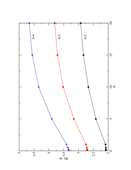
Figure 7: Re $\omega$ as a function of Gauss-Bonnet coupling $\alpha$ for $l=2,3,4$ and $n=0$ in $d=8$ for vector perturbations.

      

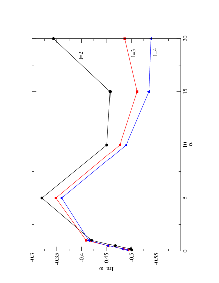
Figure 8: Im $\omega$ as a function of Gauss-Bonnet coupling $\alpha$ for $l=2,3,4$ and $n=0$ in $d=7$ for vector perturbations.

          

2b. Charged Gauss-Bonnet Black Hole

The charged Gauss-Bonnet black hole has the following form of $f(r)$ [23]:

$$f(r)=1+\frac{r^{2}}{2\alpha}-\frac{r^{2}}{2\alpha}\sqrt{1+\frac{8\alpha M}{r^{d-1}}-\frac{4\alpha Q^{2}}{2\pi(d-2)(d-3)r^{2d-4}}},$$ (2.21)

if $M>0$ and $\alpha>0$, then there will be a timelike singularity which will be shielded by two horizons if $Q<Q_{ex}$. Here $Q_{ex}$ is the extremal value of the charge determined from [23]:

$$r_{ex}^{2(d-3)}+\frac{d-5}{d-3}\alpha r_{ex}^{2(d-4)}-\frac{Q_{ex}^{2}}{2\pi(d-2)(d-3)}=0,$$ (2.22)

where,

$$r_{ex}^{d-3}=-\frac{1}{2}(d-5)M+\left[\frac{1}{4}(d-5)^{2}M^{2}+\frac{(d-4)Q_{ex}^{2}}{2\pi(d-2)(d-3)}\right]^{1/2}.$$ (2.23)

$Q$	$\omega$
	d=7	d=8
1.0	2.16438-0.44078i	2.63435-0.54628i
2.0	2.16556-0.43951i	2.63485-0.54543i
3.0	2.16750-0.43731i	2.63566-0.54400i
4.0	2.17016-0.43411i	2.63677-0.54196i
5.0	2.17347-0.42977i	2.63814-0.53929i
6.0	2.17730-0.42414i	2.63971-0.53596i
7.0	2.18137-0.41711i	2.64143-0.53194i

Table 8: Quasinormal frequency of charged Gauss Bonnet Black Hole for $\alpha=1$, $l=2$ and $n=0$ in $d=7,8$ for tensor perturbations.

For $Q=Q_{ex}$, there is a single degenerate horizon at $r=r_{ex}$. For the charged case, we find that the real part of the frequency is just increasing and the damping is decreasing as the charge of the black hole is increased. In Table 8, we give the quasinormal frequencies of the charged Gauss-Bonnet black hole with the charge of the black hole (normalized by the extremal value of the charge) for $\alpha=1$, $l=2$ and $n=0$.

In Figure (10) and (11) the real and imaginary part of the quasinormal frequency is plotted as a function of $Q/Q_{ex}$. This nature is also quite similar to that obtained by Konoplya [33] while discussing the scalar perturbation of the charged Gauss-Bonnet black hole.

      

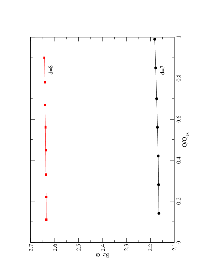
Figure 10: Plot of Re $\omega$ vs. $Q/Q_{ex}$ for charged Gauss-Bonnet black hole in $d=7$ and $8$ where $\alpha=1$, $l=2$ and $n=0$

          

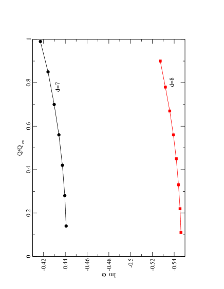
Figure 11: Plot of Im $\omega$ vs. $Q/Q_{ex}$ for charged Gauss-Bonnet black hole in $d=7$ and $8$ where $\alpha=1$, $l=2$ and $n=0$

3.  Discussion

We have obtained the QN frequencies for tensor type perturbations of the uncharged Gauss-Bonnet black hole in five, seven and eight dimensions using the tensor type gravitational potential derived in [36]. We have also obtained the QN frequencies for vector type perturbations [37] of the same black hole in five, six, seven and eight dimensions. We have shown that in the limit $\alpha\to 0$, one gets the QN frequency for the tensor type as well as vector type perturbations of the Schwarzschild black hole. This indicates that when the Gauss-Bonnet coupling $\alpha$ goes to zero, results of Einstein gravity can be reproduced. The case for $d=6$ is ruled out in case of tensor type perturbations because of the fact that it is unstable to tensorial perturbations [36]. We observe that the real and imaginary part of the QN frequencies depend on the Gauss-Bonnet coupling $\alpha$ for both the cases. The real oscillation frequency for tensor and vector type perturbations always increases with the increase of the GB coupling $\alpha$. The damping decreases as we increase the Gauss-Bonnet coupling, but after reaching certain value of $\alpha$ the damping increases. Though our results for the QN frequencies of tensor perturbations matches qualitatively with the results for quasinormal frequencies arising due to scalar field perturbations [33], the values of the QN frequencies are different.

We have also discussed about the nature of QN frequency of the charged GB black hole under tensor perturbations. The QN frequencies of the charged Gauss-Bonnet black hole for vector perturbations were difficult to find out because of the computational complicacy. It has been found that the real part of the frequency increases and the imaginary part decreases with the increase of charge for the tensor perturbation case.

The problem of finding asymptotically highly damped QNMs is beyond our study. The study of asymptotic QNMs of higher dimensional Schwarzschild black hole with a Gauss-Bonnet correction was done in [51], but the investigation of asymptotic QNMs for the full Gauss-Bonnet metric still remains incomplete.

4.  Acknowledgement

The author wishes to thank Kumar S. Gupta for numerous discussions and comments during the work and for carefully reading the manuscript.

References

- [1] Kokkotas, K.D., Schmidt, B.G.: Living Rev. Rel. 2, 2 (1999)
- [2] Nollert, H.-P.: Class. Quantum Grav. 16, R159 (1999)
- [3] Regge, T., Wheeler, J.A.: Phys. Rev. 108, 1063 (1957)
- [4] Zerilli, F.J.: Phys. Rev. D2, 2141 (1970)
- [5] Vishveshwara, C.V.: Phys. Rev. D1, 2870 (1970)
- [6] Vishveshwara, C.V.: Nature, 227 936 (1970)
- [7] Kokkotas, K.D., Stergioulas, N.: Proc. th Int. Workshop on New Worlds in Astroparticle Physics, Faro, Portugal, - January, 2005, eds. Mourao, A.M. et al (World Scientific, Singapore, 2006)
- [8] Birmingham, D., Sachs, I., Solodukhin, S.N.: Phys. Rev. Lett. 88, 151301 (2002)
- [9] Birmingham, D., Sachs, I., Solodukhin, S.N.: Phys. Rev. D67, 104026 (2003)
- [10] Hod, S.: Phys. Rev. Lett. 81, 4293 (1998)
- [11] Dreyer, O.: Phys. Rev. Lett. 90, 081301 (2003)
- [12] Motl, L., Neitzke, A.: Adv. Theor. Math. Phys. 7, 307 (2003)
- [13] Das, S., Shankaranarayanan, S.: Class. Quantum Grav. 22, L7 (2005)
- [14] Ghosh, A., Shankaranarayanan, S., Das, S.: Class. Quantum Grav. 23, 1851 (2006)
- [15] Natário, J., Schiappa, R.: Adv. Theor. Math. Phys. 8, 1001 (2004)
- [16] Sen, A.: JHEP 0603, 008 (2006)
- [17] Moura, F., Schiappa, R.: Class. Quantum Grav. 24, 361 (2007)
- [18] Scherk, J., Schwarz, J.H.: Nucl. Phys. B81, 118 (1974)
- [19] Zwiebach, B.: Phys. Lett B156, 315 (1985)
- [20] Boulware, D.G., Deser, S.: Phys. Rev. Lett. 55, 2656 (1985)
- [21] Wheeler, J.T.: Nucl. Phys. B268, 737 (1986)
- [22] Wheeler, J.T.: Nucl. Phys. B273, 732 (1986)
- [23] Wiltshire, D.L.: Phys. Rev. D38, 2445 (1988)
- [24] Meissner, K.A., Olechowski, M.: Phys. Rev. D65, 064017 (2002)
- [25] Cvetic, M., Nojiri, S., Odintsov, S.D.: Nucl. Phys. B628, 295 (2002);
- [26] Nojiri, S., Odintsov, S.D., Ogushi, S,: Phys. Rev. D65, 023521 (2002)
- [27] Cho, Y.M., Neupane, I.P.: Phys. Rev. D66, 024044 (2002);
- [28] Neupane, I.P.: Phys. Rev. D67, 061501 (2003)
- [29] Cai, R.G.: Phys.Lett. B582, 237 (2004)
- [30] Clunan, T., Ross, S.F., Smith, D.J.: Class. Quantum Grav. 21, 3447 (2004)
- [31] Barrau, A., Grain, J., Alexeyev, S.O.: Phys. Lett. B584, 114 (2004)
- [32] Iyer, B.R., Iyer, S., Vishveshwara, C.V.: Class. Quantum Grav. 6, 1627 (1989)
- [33] Konoplya, R.: Phys. Rev. D71, 024038 (2005)
- [34] Abdalla, E., Konoplya, R.A., Molina, C.: Phys. Rev. D72, 084006 (2005)
- [35] Iyer, S.: Phys. Rev. D35, 3632 (1987)
- [36] Dotti, G., Gleiser, R.J.: Class. Quantum Grav. 22 L1, (2005)
- [37] Gleiser, R.J., and Dotti, G.: Phys. Rev. D72, 124002 (2005)
- [38] Higuchi, A.: J. Math. Phys. 28, 1553 (1987)
- [39] Rubin, M.A., Ordóñez, C.R.: J. Math. Phys. 25, 2888 (1984)
- [40] Ishibashi, A., Kodama, H.: Prog. Theor. Phys. 110, 701 (2003)
- [41] Kodama, H., Ishibashi, A.: Prog. Theor. Phys. 110, 901 (2003)
- [42] Chandrasekhar, S., Detweiler, S.: Proc. Roy. Soc.(London) A344, 441 (1975)
- [43] Ferrari, V., Mashhoon, B.: Phys. Rev. D30, 295 (1984)
- [44] Schutz, B., Will, C.M.: Astrophys. J. 291, L33 (1988)
- [45] Iyer, S., Will, C.M.: Phys. Rev D35, 3621 (1985)
- [46] Konoplya, R.A.: Phys. Rev. D68, 024018 (2003)
- [47] Andersson, N.: Proc. R. Soc. (London) A439, 47 (1992);
- [48] Andersson, N., Linnaeus, S.: Phys. Rev. D46, 4179 (1992)
- [49] Leaver, E.W.: Proc. R. Soc. (London) A402, 285 (1985)
- [50] Cardoso, V., Lemos, J.P.S., Yoshida, S.: Phys. Rev. D69, 044004 (2004)
- [51] Chakrabarti, S.K., Gupta, K.S.: Int. J. Mod. Phys. A21, 3565 (2006)
- [52] Konoplya, R.A.: Phys. Rev. D68, 124017 (2003)