$\theta$ dependence of the spectrum of SU($N$) gauge theories

Abstract:

We study the $\theta$ dependence of the spectrum of four-dimensional SU($N$) gauge theories, where $\theta$ is the coefficient of the topological term in the Lagrangian, for $N\geq 3$ and in the large-$N$ limit. We compute the $O(\theta^{2})$ terms of the expansions around $\theta=0$ of the string tension and the lowest glueball mass, respectively $\sigma(\theta)=\sigma\left(1+s_{2}\theta^{2}+...\right)$ and $M(\theta)=M\left(1+g_{2}\theta^{2}+...\right)$, where $\sigma$ and $M$ are the values at $\theta=0$. For this purpose we use numerical simulations of the Wilson lattice formulation of SU($N$) gauge theories for $N=3,4,6$. The $O(\theta^{2})$ coefficients turn out to be very small for all $N\geq 3$. For example, $s_{2}=-0.08(1)$ and $g_{2}=-0.06(2)$ for $N=3$. Their absolute values decrease with increasing $N$. Our results are suggestive of a scenario in which the $\theta$ dependence in the string and glueball spectrum vanishes in the large-$N$ limit, at least for sufficiently small values of $|\theta|$. They support the general large-$N$ scaling arguments that indicate $\bar{\theta}\equiv\theta/N$ as the relevant Lagrangian parameter in the large-$N$ expansion.

1 Introduction

Four-dimensional SU($N$) gauge theories have a nontrivial dependence on the angle $\theta$ that appears in the Euclidean Lagrangian as

$${\cal L}_{\theta}={1\over 4}F_{\mu\nu}^{a}(x)F_{\mu\nu}^{a}(x)-i\theta{g^{2}\over 64\pi^{2}}\epsilon_{\mu\nu\rho\sigma}F_{\mu\nu}^{a}(x)F_{\rho\sigma}^{a}(x)$$ (1)

($q(x)=\frac{g^{2}}{64\pi^{2}}\epsilon_{\mu\nu\rho\sigma}F_{\mu\nu}^{a}(x)F_{\rho\sigma}^{a}(x)$ is the topological charge density). Indeed, the most plausible explanation of how the solution of the so-called U(1)_A problem can be compatible with the $1/N$ expansion (performed keeping $g^{2}N$ fixed [1]) requires a nontrivial $\theta$ dependence of the ground-state energy density $F(\theta)$,

$$F(\theta)=-{1\over V}\ln\int[dA]\exp\left(-\int d^{d}x{\cal L}_{\theta}\right),$$ (2)

in the $d$-dimensional pure gauge theory to leading order in $1/N$ [2, 3]. The large-$N$ ground-state energy is expected to behave as [4, 5, 6]

$$\Delta F(\theta)\equiv F(\theta)-F(0)={\cal A}\,\theta^{2}+O\left(1/N^{2}\right)$$ (3)

for sufficiently small values of $\theta$, i.e. $\theta<\pi$. This has been supported by Monte Carlo simulations of the lattice formulation of SU($N$) gauge theories [7]. Indeed, the numerical results for $N=3,4,6$ are consistent with a scaling behavior around $\theta=0$ given by

$$f(\theta)\equiv\sigma^{-2}\Delta F(\theta)={1\over 2}C\theta^{2}(1+b_{2}\theta^{2}+...),$$ (4)

$$C=C_{\infty}+c_{2}/N^{2}+...,\qquad b_{2}=b_{2,2}/N^{2}+...$$

where $\sigma$ is the string tension at $\theta=0$. $C$ is the ratio $\chi/\sigma^{2}$ where $\chi=\int d^{4}x\langle q(x)q(0)\rangle$ is the topological susceptibility at $\theta=0$. Its large-$N$ limit $C_{\infty}$ is [7, 8] $C_{\infty}\approx 0.022$. Moreover, estimates of $c_{2}$ and $b_{2,2}$ are [7] $c_{2}\approx 0.06$, and $b_{2,2}\approx-0.2$ ($b_{2}\approx-0.02$ for SU(3) [7, 9]). Note that Eq. (4) can be recast in the form

$$f(\theta)=N^{2}\bar{f}(\bar{\theta}\equiv\theta/N),$$ (5)

$$\bar{f}(\bar{\theta})={1\over 2}C\bar{\theta}^{2}(1+\bar{b}_{2}\bar{\theta}^{2}+...),$$

where $\bar{b}_{2}=b_{2,2}+O(1/N^{2})=O(1)$. This is consistent with general large-$N$ scaling arguments applied to the Lagrangian (1), which indicate $\bar{\theta}\equiv\theta/N$ as the relevant Lagrangian parameter in the large-$N$ limit of the ground-state energy [4].

Another interesting issue concerns the $\theta$ dependence of the spectrum of the theory. This is particularly interesting in the large-$N$ limit where the issue may also be addressed by other approaches, such as AdS/CFT correspondence applied to nonsupersymmetric and non conformal theories, see e.g. Ref. [10]. The analysis of the $\theta$ dependence of the glueball spectrum using AdS/CFT suggests that the only effect of the $\theta$ term in the leading large-$N$ limit is that the lowest spin-zero glueball state becomes a mixed state of $0^{++}$ and $0^{-+}$ glueballs, as a consequence of the fact that the $\theta$ term breaks parity, but its mass does not change [11].

In this paper we present an exploratory numerical study of the $\theta$ dependence in the spectrum of SU($N$) gauge theories. For this purpose we use numerical simulations of the Wilson lattice formulation. Numerical Monte Carlo studies of the $\theta$ dependence are made very difficult by the complex nature of the $\theta$ term. In fact the lattice action corresponding to the Lagrangian (1) cannot be directly simulated for $\theta\neq 0$. Here we restrict ourselves to the region of relatively small $\theta$ values, where one may expand the observable values around $\theta=0$. We consider the string tension and the lowest glueball mass. We write

$$\sigma(\theta)=\sigma\left(1+s_{2}\theta^{2}+...\right),$$ (6)

where $\sigma$ is the string tension at $\theta=0$. When $N\geq 4$ analogous expressions can be written for the other independent $k$-strings associated with group representations of higher $n$-ality. Moreover, for the lowest glueball state we write

$$M(\theta)=M\left(1+g_{2}\theta^{2}+...\right)$$ (7)

where $M$ is the $0^{++}$ glueball mass at $\theta=0$. Then the coefficients of these expansions can be computed from appropriate correlators at $\theta=0$. The $O(\theta^{2})$ coefficients $s_{2}$ and $g_{2}$ are dimensionless quantities, which should approach a constant in the continuum limit, with $O(a^{2})$ scaling corrections. The idea is analogous to the one exploited in Ref. [7] to study the $\theta$-dependence of the ground-state energy.

We shall present results for four-dimensional SU($N$) gauge theories with $N=3,4,6$. The estimates of the $O(\theta^{2})$ coefficients turn out to be very small for all $N\geq 3$. For example $s_{2}=-0.08(1)$ and $g_{2}=-0.06(2)$ for $N=3$. Moreover, their absolute values decrease with increasing $N$. We also observe that the $O(\theta^{2})$ terms are substantially smaller in dimensionless ratios such as $M/\sqrt{\sigma}$ and, for $N>3$, the ratios of independent $k$ strings, $R_{k}=\sigma_{k}/\sigma$. Our results are suggestive of a large-$N$ scenario in which the $\theta$ dependence in the string and glueball spectrum vanishes around $\theta=0$. They are consistent with the general large-$N$ scaling arguments indicating $\bar{\theta}\equiv\theta/N$ as the relevant parameter in the large-$N$ limit. We also show that a similar scenario emerges in the two-dimensional CP^N-1 models by an analysis of their $1/N$ expansion.

The paper is organized as follows. In Sec. 2 we outline the numerical method to estimate the $O(\theta^{2})$ terms of the expansion in powers of $\theta$ around $\theta=0$. The results of our exploratory numerical study are presented in Sec. 3. Finally, in Sec. 4 we discuss the $\theta$ dependence of two-dimensional CP^N-1 models within their $1/N$ expansion around their large-$N$ saddle-point solution.

2 Numerical method

2.1 Monte Carlo simulations

We consider the Wilson formulation of lattice gauge theories:

$$S=-N\beta\sum_{x,\mu>\nu}{\rm Tr}\left[U_{\mu}(x)U_{\nu}(x+\mu)U_{\mu}^{\dagger}(x+\nu)U_{\nu}^{\dagger}(x)+{\rm h.c.}\right],$$ (8)

where $U_{\mu}(x)\in$ SU($N$) are link variables. In our simulations we employed the Cabibbo-Marinari algorithm [12] to upgrade SU($N$) matrices by updating their SU(2) subgroups (we selected $N(N-1)/2$ subgroups and each matrix upgrading consists of $N(N-1)/2$ SU(2) updatings). This was done by alternating microcanonical over-relaxation and heat-bath steps, typically in a 4:1 ratio.

Computing quantities related to topology using lattice simulation techniques is not a simple task. In a lattice theory the fields are defined on a discretized set, therefore the topological properties are strictly trivial. One relies on the fact that the physical topological properties are recovered in the continuum limit. Various techniques have been proposed and employed to associate a topological charge $Q$ to a lattice configuration, see, e.g, Refs. [13, 14] for techniques based on bosonic operators, and Refs. [15, 16] for techniques based on fermionic estimators. The most robust definition of topology on the lattice is the one obtained using the index of the overlap Dirac operator. However, due to the computational cost of fermionic methods and the need for very large statistics to measure correlations of Polyakov and plaquette operators with topological quantities, we decided to use the simpler cooling method, implemented as in Ref. [7]. Direct comparison with a fermionic estimator is known to show a good agreement in the case of SU(3) [15, 7, 17], supporting the idea that the cooling method is fairly stable in this case. Moreover, the agreement among different methods is expected to improve with increasing $N$ [18, 19].

A severe form of critical slowing down affects the measurement of $Q$, posing a serious limitation for numerical studies of the topological properties in the continuum limit, especially at large values of $N$. The autocorrelation time $\tau_{Q}$ of the topological modes rapidly increases with the length scale, much faster than the standard square law of random walks [7, 20]. The available estimates of $\tau_{Q}$ appear to increase as an exponential of the length scale, or with large power laws. A qualitative explanation of this severe form of critical slowing down may be that topological modes give rise to sizeable free-energy barriers separating different regions of the configuration space. As a consequence, the evolution in configuration space may present a long-time relaxation due to transitions between different topological charge sectors. This dramatic effect has not been observed in plaquette-plaquette or Polyakov line correlations, suggesting an approximate decoupling between topological modes and nontopological ones, such as those determining the confining properties and the glueball spectrum. But, as we shall see, such a decoupling is not complete. Therefore the strong critical slowing down that is clearly observed in the topological sector will eventually affect also the measurements of nontopological quantities, such as those related to the string and glueball spectrum.

2.2 The $O(\theta^{2})$ coefficients of the $\theta$ expansion

In this subsection we describe the method to determine the $O(\theta^{2})$ coefficients of the $\theta$ expansions such as Eqs. (6) and (7). Let us first discuss the case of the fundamental string tension. The string tension can be determined from the torelon mass, i.e. the mass describing the large-time exponential decay of the wall-wall correlations $G_{P}$ of Polyakov lines [21]. In the presence of a $\theta$ term,

$$G_{P}(t,\theta)=\langle A_{P}(t)\rangle_{\theta}={\int[dU]A_{P}(t)e^{-\int d^{4}x{\cal L}_{\theta}}\over\int[dU]e^{-\int d^{4}x{\cal L}_{\theta}}}$$ (9)

where

$$A_{P}(t)=\sum_{x_{1},x_{2}}{\rm Tr}\,P(0;0)\;{\rm Tr}\,P(x_{1},x_{2};t),$$ (10)

and $P(x_{1},x_{2};t)$ is the Polyakov line along the $x_{3}$ direction of size $L$. The time separation $t$ is an integer multiple of the lattice spacing $a$: $t=n_{t}\,a$. The correlation $G_{P}$ can be expanded in powers of $\theta$. Here, we are considering the case of the fundamental string tension, but the discussion can be easily extended to any other group representation, by replacing the trace with the corresponding character in Eq. (10). Taking into account the parity symmetry at $\theta=0$, we obtain

$$G_{P}(t,\theta)=G_{P}^{(0)}(t)+\frac{1}{2}\theta^{2}G_{P}^{(2)}(t)+O(\theta^{4}),$$ (11)

where

$$G_{P}^{(0)}(t)=\langle A_{P}(t)\rangle_{\theta=0},$$ (12)

$$G_{P}^{(2)}(t)=-\langle A_{P}(t)Q^{2}\rangle_{\theta=0}+\langle A_{P}(t)\rangle_{\theta=0}\langle Q^{2}\rangle_{\theta=0}$$ (13)

and $Q$ is the topological charge.

The correlation function $G_{P}$ is expected to have a large-$t$ exponential behavior

$$G_{P}(t,\theta)\approx B(\theta)e^{-E(\theta)t},$$ (14)

where $E(\theta)$ is the $\theta$-dependent energy of the lowest state (torelon mass), and $B(\theta)$ is the overlap of the source with the lowest-energy state. If the lattice size $L$ is sufficiently large, the lowest-energy states describing the long-distance behavior of Polyakov correlators should be those of a string-like spectrum. Then, the string tension is extracted using the relation

$$E(\theta)=\sigma(\theta)L-{\pi\over 3L}$$ (15)

Here we are assuming that the $O(1/L)$ (Lüscher) correction is independent of $\theta$. Actually we are also assuming the so called free string spectrum

$$W_{n}=\sigma L\left(1-{\pi\over 3l_{\sigma}^{2}}+n{4\pi\over l_{\sigma}^{2}}\right),\qquad l_{\sigma}\equiv\sqrt{\sigma}L$$ (16)

($n$: excitation level), obtained neglecting the self-interaction terms in the string effective action, see e.g. Ref. [22]. As shown in Ref. [22], only the $O(1/L)$ correction should be universal, while subleading corrections are generally expected. They depend on the unknown coefficients of the higher order terms of the effective QCD string action. For example, besides the free string spectrum, one may also consider the Nambu-Goto string spectrum [22, 23]

$$W_{n}=\sigma L\left(1-{2\pi\over 3l_{\sigma}^{2}}+n{8\pi\over l_{\sigma}^{2}}\right)^{1/2}$$ (17)

In particular, if one assumes the Nambu-Goto spectrum, instead of Eq. (15), one should use the Nambu-Goto lowest-energy state to determine the string tension, i.e.

$$W_{0}=\sigma L\left(1-{2\pi\over 3l_{\sigma}^{2}}\right)^{1/2}=\sigma L\left[1-{\pi\over 3l_{\sigma}^{2}}-{\pi^{2}\over 18l_{\sigma}^{4}}+O\left({1/l_{\sigma}^{6}}\right)\right]$$ (18)

Therefore the Nambu-Goto string spectrum leads to a different estimate of the string tension at finite $l_{\sigma}$:

$$\sigma_{\rm fs}=\sigma_{\rm NG}\left[1-{\pi^{2}\over 18l_{\sigma}^{4}}+O(l_{\sigma}^{-6})\right]$$ (19)

where $\sigma_{\rm fs}$ and $\sigma_{\rm NG}$ are the string tensions extracted from the torelon mass assuming respectively the free and Nambu-Goto spectrum.

Lattice sizes such that $l_{\sigma}\gtrsim 3$ should be sufficiently large to have an effective string picture parametrized by a constant string tension $\sigma$ [24]. Then the different estimates of $\sigma$ obtained by using the free and Nambu-Goto spectra might provide an estimate of systematic error on the determination of $\sigma$ from the lowest torelon mass due to our partial knowledge of the effective QCD string action. For $l_{\sigma}=3$ one has $\sigma_{\rm NG}/\sigma_{\rm fs}-1\approx 0.007$.

We expand the large-$t$ behavior (14) of $G(t,\theta)$ as

$$G_{P}(t,\theta)\approx B_{0}e^{-E_{0}t}\left[1+\theta^{2}h(t)+...\right]$$ (20)

where we set

$$B(\theta)=B_{0}+\theta^{2}B_{2}+...,$$ (21)

$$E(\theta)=E_{0}+\theta^{2}E_{2}+...,$$ (22)

and

$$h(t)=\frac{B_{2}}{B_{0}}-E_{2}t$$ (23)

Comparing the Eq. (20) with the Eq. (13), we find that

$$h(t)={G^{(2)}_{2}(t)\over 2G^{(0)}(t)}$$ (24)

Thus $E_{2}$ can be estimated from the difference

$$\Delta h(t)=h(t)-h(t+a),$$ (25)

indeed

$${\displaystyle\lim_{t\to\infty}}\;\Delta h(t)=E_{2}\,a$$ (26)

Corrections are exponentially suppressed as $\exp[-(E^{*}_{0}-E_{0})t]$ where $E^{*}_{0}$ is the mass of the first excited state at $\theta=0$. Assuming the free-string spectrum (16), $E^{*}_{0}-E_{0}=4\pi/L$. Notice that, although $E^{*}_{0}-E_{0}\rightarrow 0$ for $L\rightarrow\infty$, this difference is not small in our calculations. Indeed, since we choose the lattice size $L$ so that $l_{\sigma}\equiv\sqrt{\sigma}L\approx 3$, $(E_{0}^{*}-E_{0})/E_{0}\approx 4\pi/l_{\sigma}^{2}\approx 1.4$.

Finally, the coefficient $s_{2}$ of the $O(\theta^{2})$ term in the expansion (6) is obtained by

$$s_{2}={E_{2}\over\sigma L}$$ (27)

$s_{2}$ is a dimensionless scaling quantity. It is expected to approach a constant in the continuum limit, with $O(a^{2})$ scaling corrections.

An analogous procedure can be used to determine the leading $O(\theta^{2})$ term in the $\theta$ expansion of the lowest glueball mass $M(\theta)$ around $\theta=0$, cf. Eq. (7). In this case we employ wall-wall correlators of plaquette-like operators with up to 6 links, all in spatial directions, in order to determine the $0^{++}$ glueball mass. Correspondingly we define

$$\Delta k(t)\equiv k(t)-k(t+a)$$ (28)

where $k(t)$ is the function analogous to $h(t)$ defined from the glueball wall-wall correlators. Then, the $O(\theta^{2})$ coefficient $g_{2}$ in the expansion (7) can be obtained by

$$g_{2}={1\over a\,M}\,\lim_{t\to\infty}\;\Delta k(t)$$ (29)

where $M$ is the $0^{++}$ glueball mass.

Finally, we mention that in order to improve the efficiency of the measurements we used smearing and blocking procedures (see, e.g., Refs. [25, 24]) to construct new operators with a better overlap with the lightest propagating state. Our implementation of smearing and blocking was already described in Ref. [26]. We only mention that we constructed new super-links using three smearing, and a few (2-4) blocking steps, according to the value of $L$. These super-links were used to compute improved Polyakov lines or plaquette operators.

3 Results

Table 1: Some information on our Monte Carlo simulations for $N=3,4,6$. The estimates of the string tension $\sigma$ are obtained using Eq. (15).

$N$	$\beta$	lattice	stat	$a^{2}\,\sigma$	$a\,M_{0^{++}}$	$M_{0^{++}}/\sqrt{\sigma}$
3	5.9	$12^{3}\times 18$	25M/20	0.0664(6)	0.80(1)	3.09(4)
3	6.0	$16^{3}\times 36$	25M/40	0.0470(3)	0.70(1)	3.23(4)
4	10.85	$12^{3}\times 18$	16M/50	0.0646(6)	0.76(1)	2.99(5)
6	24.5	$8^{3}\times 12$	9M/50	0.114(2)	0.83(1)	2.46(4)

In this section we present the results of our exploratory study of the $\theta$ dependence of the spectrum using the method outlined in the preceding section. Table 1 contains some information on our MC runs for $N=3,4,6$ on lattices $L^{3}\times T$. Since the coefficients of the $\theta$ expansions (6) and (7) are computed from connected correlation functions, such as (13), and turn out to be quite small, high statistics is required to distinguish their estimates from zero: Our runs range from 9 to 25 million sweeps, with measures taken every 20-50 sweeps. This requirement represents a serious limitation to the possibility of performing runs for large lattices and in the continuum limit, especially for large values of $N$, due also to the severe critical slowing down discussed in Sec. 2.1. For all values of $\beta$ considered in this work, the autocorrelation time satisfies $\tau_{Q}\lesssim 100$ sweeps [7]. Furthermore, $\beta$ values were chosen to lie in the weak-coupling region, i.e., beyond the first order phase transition in the case $N=6$, and beyond the crossover region characterized by a peak of the specific heat for $N=3,4$; see Ref. [26] for a more detailed discussion of this point. Runs generally started from cold configurations, to avoid problems due to metastable states at the transition (in the case $N=6$). The lattice size $L$ was chosen so that $l_{\sigma}\equiv\sqrt{\sigma}L\gtrsim 3$, which should be sufficiently large to obtain infinite-volume results (see, e.g., Refs. [24, 26]), at least within our precision. Due to the above-mentioned limitations, and in particular for $N=4,6$ we could afford only one value of $\beta$, so that no stringent checks of scaling could be performed. For this reason our study should be still considered as a first exploratory investigation.

Figure 1: Plot of $\Delta h(t)$ and $\Delta k(t)$ for $N=3$ at $\beta=5.9$ (above) and $\beta=6.0$ (below). The data for $\Delta k(t)$ are slightly shifted along the $t$ axis.

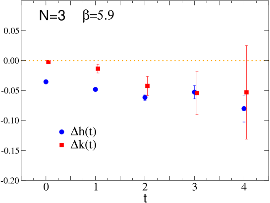
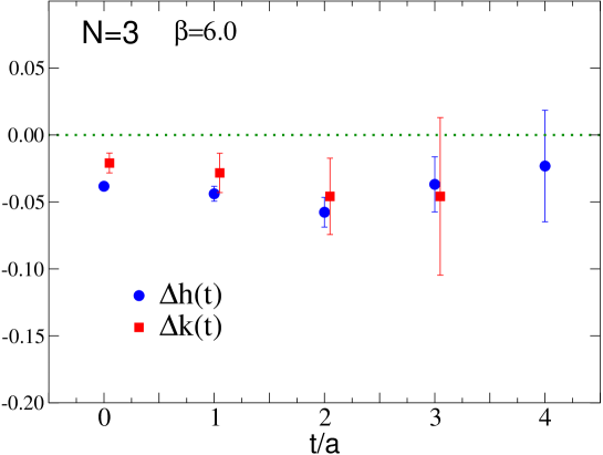
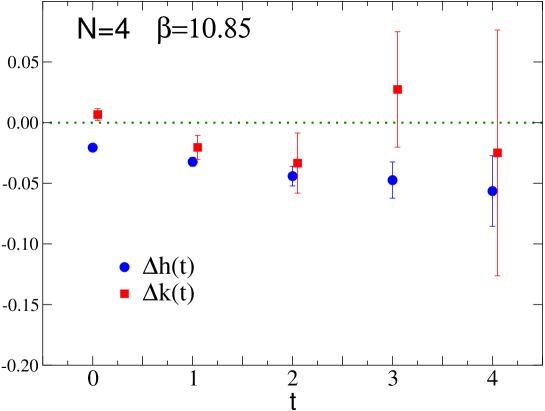
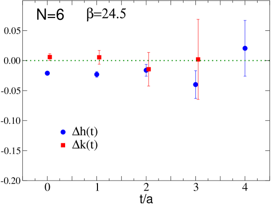
Figs. 1 and 2 show the results for the discrete differences $\Delta h(t)$ and $\Delta k(t)$, cf. Eqs. (25) and (28), for $N=3$ at $\beta=5.9,6.0$ and for $N=4,6$ respectively. As expected, the signal degrades rapidly with increasing $t$. Anyway, they appear rather stable already for small values of $t$. As already discussed in Sec. 2.2, the approach to a constant in the large-$t$ limit should be exponential, as $\exp[-(E^{*}_{0}-E_{0})t]$, where $E^{*}_{0}$ is the energy of the first excited state at $\theta=0$. In the case $N=3$ the data at $\beta=6$ appear to approach the asymptotic behavior more rapidly than at $\beta=5.9$. This should be due to the fact that a more effective blocking procedure can be applied when $L=16$, rather than $L=12$, achieving a better overlap with the lowest state.

We estimate the coefficients $s_{2}$ and $g_{2}$ of the $O(\theta^{2})$ terms in the expansions (6) and (7) from the corresponding discrete differences $\Delta h(t)$ and $\Delta k(t)$ [cf. Eqs. (26), (27), and (29)], taking the data at $t/a=2$ in the $N=3,4$ runs, and at $t/a=1$ for $N=6$. In Table 2 we report the results. The estimates of $s_{2}$ and $g_{2}$ are small in all cases, and decrease with increasing $N$. For $N=3$ the results at $\beta=5.9$ and $\beta=6.0$ are consistent, supporting the expected scaling behavior. As final estimate one may consider

$$s_{2}=-0.08(1),\quad g_{2}=-0.06(2)\qquad{\rm for}\;\;N=3$$ (30)

Figure 2: Plot of $\Delta h(t)$ and $\Delta k(t)$ for $N=4$ at $\beta=10.85$ (above) and $N=6$ at $\beta=24.5$ (below). The data for $\Delta k(t)$ are slightly shifted along the $t$ axis.

One may also consider the $\theta$ dependence of the scaling ratio

$${M(\theta)\over\sqrt{\sigma(\theta)}}={M\over\sqrt{\sigma}}(1+c_{2}\theta^{2}+...),$$ (31)

where $c_{2}=g_{2}-s_{2}/2$. Using the numbers reported in Table 2, we see that the $O(\theta^{2})$ terms tend to cancel in the ratio. Indeed, we find $c_{2}=-0.02(2),\,-0.01(3),\,-0.01(2)$ respectively for $N=3,4,6$.

For $N=4,6$ there are other independent $k$-strings associated with representations of higher $n$-ality. Analogously to the fundamental string, one may write

$$\sigma_{k}(\theta)=\sigma_{k}\left(1+s_{k,2}\,\theta^{2}+...\right),$$ (32)

where $\sigma_{k}$ is the $k$-string tension at $\theta=0$. The case $k=1$ corresponds to the fundamental string tension, i.e. $\sigma_{1}\equiv\sigma$ and $s_{1,2}\equiv s_{2}$. One may also consider the ratio $R_{k}=\sigma_{k}/\sigma$,

$$R_{k}(\theta)=R_{k}\left(1+r_{k,2}\,\theta^{2}+...\right),$$ (33)

where $R_{k}$ is the ratio at $\theta=0$ (see e.g. Refs. [24, 26, 27, 28] for recent numerical studies of the $k$-string spectrum), and $r_{k,2}=s_{k,2}-s_{2}$. In the case $N=4$ there is one independent $k$ string, $\sigma_{2}$, besides the fundamental one; in the case $N=6$ there are two. Our results for the $k>1$ strings are less stable. We obtained sufficiently precise results only from the simulation for $N=4$. In the channel of Polyakov lines corresponding to the $k=2$ string, we found $a^{2}\sigma_{2}=0.091(2)$, $\Delta h_{2}(t/a=1)=-0.044(13)$, while at distance $t/a=2$ the signal was already unreliable. This leads to the estimate $s_{2,2}=-0.040(12)$. Note that $s_{2,2}\approx s_{1,2}$ ($s_{1,2}\equiv s_{2}$ is reported in Table 2), suggesting an even smaller $O(\theta^{2})$ term in the ratio $R_{2}$, i.e. $|r_{2,2}|\lesssim 0.02$.

Table 2: Results for the coefficients $s_{2}$ and $g_{2}$, as derived from the discrete differences at distance $t/a=2$ for $N=3,4$, and at $t/a=1$ for $N=6$.

$N$		$\beta$		$s_{2}$	$g_{2}$
3		5.9		$-$0.077(8)	$-$0.05(2)
3		6.0		$-$0.077(15)	$-$0.07(4)
4		10.85		$-$0.057(10)	$-$0.04(3)
6		24.5		$-$0.025(5)	0.006(15)

In conclusion, the above results show that the $O(\theta^{2})$ terms in the expansion around $\theta=0$ of the spectrum of SU($N$) gauge theories are very small, especially when dimensionless ratios are considered. Moreover, they appear to decrease with increasing $N$, and the coefficients do not show evidence of convergence to a nonzero value. This is suggestive of a scenario in which the $\theta$ dependence of the spectrum disappears in the large-$N$ limit, at least for sufficiently small values of $\theta$ around $\theta=0$. General large-$N$ scaling arguments applied to the Lagrangian (1) indicate $\bar{\theta}\equiv\theta/N$ as the relevant Lagrangian parameter in the large-$N$ limit [4]. In the case of the spectrum, this would imply that $O(\theta^{2})$ coefficients should decrease as $1/N^{2}$. This is roughly verified by our results, taking also into account that they may be subject to scaling corrections, especially those at $N=4,6$. For example, in the case of the string tension, $s_{2}\approx s_{2,2}/N^{2}$ with $s_{2,2}\approx-0.9$ . Of course, further investigations are required to put this scenario on a firmer ground.

The hypothesis of a simple $\theta$ dependence in the large-$N$ limit may be extended to finite temperature, up to the first-order transition point. Recent studies [29, 30] have shown that in the large-$N$ limit the topological properties remain substantially unchanged up to the first-order transition point.

4 $\theta$ dependence in the two-dimensional CP^N-1 model

Issues concerning the $\theta$ dependence can also be discussed in two-dimensional CP^N-1 models [31, 32], which are an interesting theoretical laboratory. Indeed they present several features that hold in QCD: asymptotic freedom, gauge invariance, existence of a confining potential between non gauge invariant states (that is eventually screened by the dynamical constituents), and non-trivial topological structure (instantons, $\theta$ vacua). Moreover, unlike SU($N$) gauge theories, a systematic $1/N$ expansion can be performed around the large-$N$ saddle-point solution [31, 32, 33].

Analogously to four-dimensional SU($N$) gauge theories, one may add a $\theta$ term to the Lagrangian, writing

$${\cal L}_{\theta}={N\over 2g}\overline{D_{\mu}z}\,D_{\mu}z+i\theta{1\over 2\pi}\,\epsilon_{\mu\nu}\,\partial_{\mu}A_{\nu},$$ (34)

where $z$ is a $N$-component complex scalar field subject to the constraint $\bar{z}z=1$, $A_{\mu}=i\bar{z}\partial_{\mu}z$ is a composite gauge field, and $D_{\mu}=\partial_{\mu}+iA_{\mu}$ is a covariant derivative. The topological charge density is $q(x)={1\over 2\pi}\,\epsilon_{\mu\nu}\,\partial_{\mu}A_{\nu}$ . Then one may study the $\theta$ dependence of the ground state and other observables. In the following we discuss this issue within the $1/N$ expansion, performed keeping $g$ fixed. Simple large-$N$ scaling arguments applied to the Lagrangian (34) indicate that the relevant $\theta$ parameter in the large-$N$ limit should be $\bar{\theta}\equiv\theta/N$.

As mass scale we consider the zero-momentum mass  $M$ defined from the small-momentum behavior of the Fourier trasformed two-point correlation function of the operator $P_{ij}(x)\equiv\bar{z}_{i}(x)z_{j}(x)$,

$$G_{P}(x-y)=\langle{\rm Tr}\,P(x)P(y)\rangle,$$ (35)

i.e. from the relation

$$\widetilde{G}_{P}(p)^{-1}=Z^{-1}[M^{2}+p^{2}+O(p^{4})]$$ (36)

where $Z$ is a renormalization constant.

Analogously to SU($N$) gauge theories, the ground state energy $F(\theta)$ depends on $\theta$. One may define a scaling ground state energy $f(\theta)$ and expand it around $\theta=0$,

$$f(\theta)\equiv M^{-2}[F(\theta)-F(0)]={1\over 2}C\theta^{2}\left(1+\sum_{n=1}b_{2n}\theta^{2n}\right)$$ (37)

where $F(\theta)$ is defined as in Eq. (2), $M$ is the mass scale at $\theta=0$, and $C,b_{j}$ are constants. $C$ is the scaling ratio $\chi/M^{2}$ at $\theta=0$, where $\chi$ is the topological susceptibility, i.e. the two-point correlation function of the topological charge density at zero momentum. The correlation function of the topological charge density, and in particular the topological susceptibility, has been computed within the $1/N$ expansion [34, 35, 36]. We have

$$C=\chi/M^{2}={1\over 2\pi N}+O(1/N^{2})$$ (38)

The coefficients $b_{2n}$ are obtained from appropriate $2n$-point correlation functions of the topological charge density operators at $\theta=0$. For example

$$b_{2}=-{\chi_{4}\over 12\chi},$$ (39)

$$\chi_{4}={1\over V}\left[\langle Q^{4}\rangle_{\theta=0}-3\left(\langle Q^{2}\rangle_{\theta=0}\right)^{2}\right],$$ (40)

where $Q=\int d^{2}x\,q(x)$ is the topological charge.

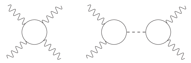
We refer to Ref. [33] for a discussion of the $1/N$ expansion within CP^N-1 models, its set up, and the list of the corresponding Feynman rules. In Fig. 3 we show the $1/N$-expansion Feynman diagrams contributing to $\chi_{4}$ at leading order. The analysis of the Feynman diagrams of the connected correlations necessary to compute $b_{2n}$ shows that they are suppressed in the large-$N$ limit, as

$$b_{2n}=O(1/N^{2n}).$$ (41)

This implies that the ground-state energy can be rewritten as

$$f(\theta)=N\bar{f}(\bar{\theta}\equiv\theta/N),$$ (42)

$$\bar{f}(\bar{\theta})={1\over 2}\bar{C}\bar{\theta}^{2}(1+\sum_{n=1}\bar{b}_{2n}\bar{\theta}^{2n}),$$

where $\bar{C}\equiv NC$ and $\bar{b}_{2n}=N^{2n}b_{2n}$ are $O(1)$ in the large-$N$ limit. Note the analogy with the expected $\theta$ dependence of the ground-state energy in SU($N$) gauge theories, cf. Eq. (5). The calculation of the coefficients of the leading large-$N$ terms is rather cumbersome. Here, we only report the results obtained for the leading terms of $\bar{b}_{2}$ and $\bar{b}_{4}$

$$\bar{b}_{2}=-{27\over 5},\qquad\bar{b}_{4}=-{1830\over 7}.$$ (43)

Within the $1/N$ expansion one may also study the dependence of the mass $M$ on the parameter $\theta$. We write

$$M(\theta)=M\left(1+m_{2}\theta^{2}+...\right)$$ (44)

The coefficient $m_{2}$ can be extracted from the connected correlations

$$\langle{\rm Tr}\,P(x)P(0)Q^{2}\rangle_{\theta=0}-\langle{\rm Tr}\,P(x)P(0)\rangle_{\theta=0}\langle Q^{2}\rangle_{\theta=0}$$ (45)

The analysis of its diagrams giving the corresponding $1/N$ expansion indicates that $m_{2}$ is suppressed as

$$m_{2}=O(1/N^{2})$$ (46)

This confirms the general large-$N$ scaling arguments indicating $\bar{\theta}\equiv\theta/N$ as the relevant parameter in the large-$N$ limit, as in the scenario put forward for the four-dimensional SU($N$) gauge theories.

Figure 3: Diagrams contributing to the four-point connected function $\chi_{4}$, cf. Eq. (40), within the $1/N$ expansion (the corresponding Feynman rules can be found in Ref. [33]).