Joakim Arnlind⋆,
Martin Bordemann∼, Laurent Hofer⋆∼,
Jens
Hoppe⋆ and Hidehiko Shimada† Department of MathematicsRoyal
Institute of TechnologyLindstedtsvägen 25S-10044 Stockholm.jarnlind@math.kth.sehoppe@math.kth.seLaboratoire de MIA4, rue des Frères LumièreUniversité de Haute-AlsaceF-68093 Mulhouse.martin.bordemann@uha.frlaurent.hofer@uha.frMax Planck Institute forGravitational Physics(Albert Einstein Institute)Am M hlenberg 1D-14476 Golm.hidehiko.shimada@aei.mpg.de
Abstract.We introduce C-Algebras (quantum analogues of
compact Riemann surfaces), defined by polynomial relations in
non-commutative variables and containing a real parameter that, when
taken to zero, provides a classical non-linear, Poisson-bracket,
obtainable from a single polynomial C(onstraint) function. For a
continuous class of quartic constraints, we explicitly work out finite
dimensional representations of the corresponding C-Algebras.
Introduction
Harmonic homogenous polynomials in 3 commuting variables, upon
substitution of -dimensional representations of for the
commuting variables, can be used to define a map from functions on
to matrices, that sends Poisson brackets to matrix
commutators [GH82]. The result was dubbed “Fuzzy Sphere”, in
[Mad92]. In [KL92] and [BMS94] it was proven
(conjectured in [BHSS91]) that the (complexified) Poisson algebra
of functions on any Riemann surface arises as a
limit of . Insight on how matrices can
encode topological information (certain sequences having been
indentifyable as converging to a particular function, but
lacking topological invariants) was gained in [Shi04]. That no
concrete anologue of the Fuzzy Sphere construction [GH82] for
higher genus compact surfaces could be found, and that the one found
for the torus [FFZ89, Hop88] was of a very different nature,
remained an unsolved puzzle, just as the rigidity of the 2
constructions. We are happy to announce a resolution by presenting a
unified (and concrete, as well as non-rigid, and intuitively
simple) treatment for general compact Riemann surfaces. In section
1 we describe Riemann surfaces of genus
embedded in as inverse images of polynomial
contraint-functions, . In section 2
we define a Poisson bracket on , to be restricted to the
embedded Riemann surface. In section 3 we review
the quantization for the round 2-sphere. In section
4 we outline our construction for general
genus. In section 5 we work out the conjectured
construction for a continuous class of tori and deformed spheres. In
section 6 we discuss how the classical singularity at
is reflected in the quantum world.
1 Genus Riemann surfaces
The aim of this section is to present compact connected
Riemann surfaces of any genus embedded in by inverse images of
polynomials. For this purpose we use the regular value theorem and
Morse theory. Let be a polynomial in 3 variables and define
. What are the conditions on , for
to be a genus Riemann surface? If is a submersion on ,
then is an orientable submanifold of . has to
be compact and of the desired genus. For further details see
[Hir76, Hof02].
The classification of 2 dimensional compact (connected) manifolds is
well known. In this case, there is a one to one correspondance between
topological and diffeomorphism classes. The result is that any compact
orientable surfaces is homeomorphic (hence diffeomorphic) to a sphere
or to a surface obtained by glueing tori together (connected sum). The
number of tori is called the genus and is related to the
Euler-Poincaré characteristic by the formula .
Morse theory
To compute we apply Morse theory to a specific
function. A point of a (smooth) function on is a
singular point if , in which case is a singular
value. At any singular point one can consider the second
derivative of and is said to be non-degenerate if
. Moreover one can attach an index to each such
point depending on the signature of : 0 if positive, 1 if
hyperbolic and 2 if negative. A Morse function is a function such that
every singular point is non-degenerated and singular values all
distinct. Then is given by the formula:
where is the number of
singular points which have an index .
The function is defined as the restriction of the first
projection on the surface. It’s not necessarily a Morse function (one
has to choose a “good” embedding for that), but the singular points
are those for which the gradient is parallel to the
axis. Moreover the Hessian matrix of at such a point is:
Polynomial model
Take
where ,
with
and . Obviously is closed and bounded (even
degree of ) hence compact. is a submanifold of if,
and only if for each , which is equivalent
to requiring that the polynomials and have only simple
roots. The singular points of the function on are the
points such that and the Hessian matrix is:
Hence it is positive or negative if, and only
if and hyperbolic if, and only if . With the
fact that can’t be zero at a singular point, it also proofs
that is a genuine Morse function. Finally,
If the polynomial has exactly 2 simple roots and the
polynomial has exactly simple roots, then
and is a surface of genus .
Explicit construction of
Let . Set:
(i)
and
(ii)
and
One can directly see that has exactly simple roots, hence
has exactly simple roots. For , the
function has no zero. On the other hand, for ,
is strictly growing and has exacly one zero. Consequently
the polynomial has exactly 2 simple roots and the surface
defined above is a genus compact Riemann surface.
2 Poisson brackets in
For arbitrary (twice continuously differentiable)
(2.1)
defines a Poisson bracket for functions on (see e.g. Nowak
[Now97] who studied the formal deformability of
(2.1))111While we did not (yet find a way to) use his results,
we are very grateful for his “New Year’s Eve” explanations, as well as
providing us with his Ph.D. Thesis..
Let be described, as in section 1,
by a “constraint”:
(2.2)
The Poisson brackets between , and then read:
(2.3)
Explicitely, substituting for , one obtains
(2.4)
resp.
(2.5)
Let , ,
be a local parametrisation of
. Restricting to a
Poisson bracket, , on the surface
, and realizing on locally as
the
relation (equivalence!, up to different constant values on the r.h.s. of
(2.4)) between (2.4) and (2.5) is
seen as follows: differentiating (2.4) with respect to the
local parameters, and , one obtains a linear
system of equations for and , whose algebraic
solution (via Cramers rule, e.g. ) gives (2.5). To go from
(2.5) to (2.4) (with the constant unspecified,
of course) one either notes simply that the l.h.s. of (2.4)
commutes with both and (according to (2.5)), or
one directly solves (2.5) via a hodograph-transformation
(cp. [BKL05], in which Poisson bracket equations are considered,
whose solutions also contain surfaces of general type222Apart from
spheres, however, these surfaces are either non-polynomial, or
non-compact – or both – causing the corresponding quantum-algebras to
be necessarily different from ours.);
changing independent variables from , to
and ; using
(deriving) (as e.g. in [BH93])
eigenfunctions of the Laplace operator on (). Write them as harmonic homogenous
polynomials in ,
and (restricted to
):
(3.1)
(where the tensor is by definition traceless and totally
symmetric), and then replace the commuting variables by
generators of the -dimensional irreducible (spin
) represensation of , to obtain -matrices:
(3.2)
automatically, for . Instead of
having equal to
(the usual normalisation), it is advantageous
to choose the normalisation ,
(3.3)
and then .
As the Poisson bracket on ,
(3.4)
can be obtained by restricting the Poisson bracket
(3.5)
to (via ), can be
computed from
(3.6)
by using the derivation property, and
(3.7)
(following from (3.5)), as well as then decomposing the
resulting polynomial of degree into harmonic homogenous ones,
to obtain the structure constants of the Lie-Poisson algebra of
functions on the -sphere (in the basis of the spherical
harmonics).
Calculating
(3.8)
the first step is identical to the one after (3.6), while
any further use of the commutation relations (3.3) –
necessary to obtain the desired traceless totally symmetric tensors –
induces factors of ; hence one finds agreement to
leading order of of the structure constants of , in the
basis , satisfying
with those of the Poisson algebra.
4 The construction for general Riemann surfaces
Let us consider compact Riemann surfaces described by
(4.1)
(with P, as in section (1), an even polynomial of degree ), resp.
(4.2)
(for (2.3)). We claim that fuzzy analogues of
can be obtained via matrix analogues of (4.1) and
(4.2). Apart from possible “explicit
corrections”, direct ordering questions arise both on the r.h.s. of
(4.2), and in (4.1), while on the l.h.s. of (4.2) one replaces Poisson brackets by
(commutator(s)).
Consider therefore the problem of
looking for matrices satisfying
(4.3)
resp.
(4.4)
(4.5)
if ; the r.h.s. of (4.5)
will also be denoted by (for a term in , e.g. ,
would correspondingly include ). This ordering in (4.4) and
(4.5) is consistent, as
(4.7)
indeed equals to zero (insert (4.4) and
(4.5) for the 2 double commutators to get ), which is has to, due to
associativity of matrix multiplication (and resulting Jacobi
identity).
Finding (for specific values of ) concrete representations of
(4.4) and (4.5), resp.(4.3), let alone classifying them, is of course a very
complicated task. We succeeded in doing so for
(corresponding to a torus when , and deformed spheres, when
, see section (5), but first we would
like to outline some qualitative features involved for the general
case. As mentioned in the introduction, one of the
puzzles was the rigidity of the construction for the round 2-sphere
[GH82] and the toral rational rotation algebra [FFZ89] (see
also [Hop89]). In the present construction we now have a
(generally, i.e. apart from certain critical values – signaling
topology change) continuous dependence on the data () which
describe the Riemann surface. For given , and , we define
the corresponding Fuzzy Riemann Surface (for fixed
, expected to exist for infinitely many discrete values of ,
coming arbitrarily close to zero) as the algebra generated by the
corresponding finite (-)dimensional solutions of
(4.4),(4.5), resp.(4.3). According to the semiclassical philosophy
explained below (cp. [Shi04]) and will exhibit eigenvalue
sequencies (generically smoothly depending on ) characteristic of
the topological type, reflecting the behaviour of the corresponding
classical embedding functions and .
Let us observe that we can read off information of topology from a
generic single function by using Morse theory. This Morse
theoretic information of topology manifests itself in the eigenvalue
distribution of the matrix corresponding to the function
:
the key idea is to introduce an auxilary Hamiltonian dynamical
system, whose phase space is the surface and whose Hamiltonian is
given by . Thus we consider ordinary differential equations
(4.8)
where parametrise the embedded surface. Since
classical orbits of (4.8) are equal- lines on the
surface, the family of the classical orbits exhibits branching
processes which exactly reflect Morse theoretic information. The
eigenvalue distribution of is determined (to leading order
in ) by the Bohr-Sommerfeld rule. That is, the
eigenvalues are values of on classical orbits which are such that
the area between adjacent orbits is equal to the total area of the
surface divided by . It follows that the eigenvalues are grouped
into subsets each corresponding to the branches on the surface. These
subsets are called in [Shi04] as eigenvalue sequences, and have
the property that (for sufficiently large ) the eigenvalues
belonging to a sequence rise in a smooth way. The branching processes
of the sequences are the same as those of the classical
orbits. Furthermore, using the eigenvalue sequences and
(4.8), a rule to calculate general (off-diagonal)
matrix elements of a matrix corresponding to a general
function was given in [Shi04]. Essential properties of the
matrix regularisation, such as the correspondence of the matrix
commutator and the Poisson bracket, can be derived from those rules.
5 Explicit solutions for tori and deformed spheres:
Representations of the simplest non-linear –Algebras
Let now which, for describes a torus, and for
a (deformed) sphere. We will construct solutions for
the corresponding matrix equations, which we take as
(5.1)
(5.2)
(5.3)
(5.4)
(in this section, denotes the anti-commutator ,
and not a Poisson-bracket).
Denoting by , one finds (using the Jacobi-identity,
the derivation property, and equations (5.2) + (5.3)) that
(5.5)
hence and commute, and can be diagonolized
simultaneously; it then also follows that is central,
i.e. commutes with and .
In complex notation, , (5.2) and (5.3) can be
written together as
(5.6)
from which the crucial commutativity of and ,
(5.7)
also follows directly (by using (5.6)). In the basis where both
and are diagonal
are the only equations relating the eigenvalue pairs.
What can we say about the possibility of coming back to
the same point after iterations, i.e
(5.14)
Multiplying by gives
(5.15)
and one deduces that either , in which case
(5.16)
– a fix point of the transformation (i.e.
, making all ’s and ’s equal to one another,
i.e. , which we don’t want) – or is a multiple
of , i.e.
(5.17)
in which case (5.14) holds for every , as then
and (the eigenvalues of are ). Expressing the constraint
(5.4) in terms of
(5.18)
giving
(5.19)
one sees that the transformation (5.10) must leave
invariant the ellipse given via (5.19). Although this becomes
obvious in the “circle-coordinates”
(5.20)
in which the transformation (5.13) between eigenvalue-pairs is simply a
rotation by ,
(5.21)
the picture of a by rotated ellipse (with halfaxes 1 and
) lying in the -plane is extremely useful,
in particular when discussing the -dependence of -dimensional representations of
eqs (5.1)–(5.4) (s.b.).
Remembering, e.g. that we get
which is only solvable if the ellipse defined by
entirely lies in the first quadrant. This observation leads to the
following: Assume that for some and let
lie on the ellipse . If
then there exists no such that and
for . If and then,
for every choice of on the ellipse, and
for all .
These solutions take the form
(5.22)
and the ellipse, on which lie, will typically look like
in Figure 1.
Figure 1: , .
In the region the set of , for which
for all , is a union of disjoint intervals whose
lengths decreases and eventually become a set of
distinct points as (however, making for some
, giving not a “loop”, but a “string” solution. This transition
will be discussed in Section 6). For a loop solution in this region,
the points will precisely “miss” the negative
region, like in Figure 2.
Figure 2: , .
For , by making a “string” Ansatz for
(5.23)
one derives, from and , the condition
, which makes the choice
necessary. Can we now, for given , find such that
? Assume that and let
.
If is a solution of
(5.24)
then and for .
There are three values of for which it is particularly easy to calculate
these solutions explicitly: and .
:
(5.25)
:
(5.26)
:
(5.27)
In the region the corresponding ellipse for a string
solution will typically look like Figure 3.
Figure 3: , and .
Let us now derive the subcritical condition for existence of
an -dimensional string representation,
(5.28)
valid for all ; with no solution for as
cannot have any nontrivial solutions. It is
useful to remember that
(5.29)
For (other values of can be
treated analogously):
(5.30)
gives
(5.31)
Let be the angle from to
:
Figure 4:
If we, by doing rotations by ,
want to go from to , we get the
condition
(5.32)
since . Rearranging (5.32), and inserting
the expression for one obtains, by taking
of both sides
(5.33)
Squaring the expression and solving for yields
(5.34)
By knowing the sign of and , we see that one of the roots
is a false root, leaving
(5.35)
For given , out of the solutions for ,
it is only the smallest that gives
the string solution; the larger ’s correspond to a total
rotation of more than (giving negative ’s).
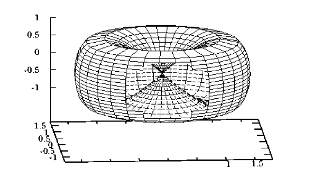
6 The singularity
Figure 5:
The equation
(6.1)
defines a regular surface, except for (the singularity being
at the origin, , see figure 5). How is this
singularity reflected in the “fuzzy world”, i.e. when looking at
finite dimensional representation of (5.1-5.4)? Interestingly,
“does exist”, for an
integer fraction of . Equations (5.1-5.4) do have, for
, (up to conjugation) a unique (“irreducible”)
dimensional solution:
(6.2)
What happens, is the following: while for large enough
(), the ellipse lies entirely in the first
quadrant of the plane (), leading to an
-dimensional representation (if ) for arbitrary
initial conditions (i.e. an arbitrary initial point on the ellipse),
this is no longer the case when approaches 1; when becomes
smaller than , and approaches from above, the
continuous range of inital conditions gradually shrinks, leaving at
precisely one “-dimensional” representation, which
however has the additional feature that in the limit () the
first row and column of , and becomes identically
zero. This drop of the dimensionality (by 1) for given
could be viewed as reflecting the singularity, while on the other
hands it cleverly (“smoothly”) leads over to the subcritical
() -dependence of .
The only representation that
survives as is the one given by
(6.3)
i.e. (the lower tip of the ellipse) as the
starting point (due to it is qualitatively
clear, that, with that initial condition one “jumps” over the small
region of negative , as well as, “at the end” the one of
negative ).
The drop in dimensionality (for ) then is
simply the vanishing of and . One could of course
relabel the points (always start with the second point, instead of the
lower tip) such that the upper block has a
smooth limit (and the row/column
“disappears” as ). As noted above, the subcritical
behaviour of as a function of (to have a
-dimensional representation) is more involved. As the allowed
part of the ellipse shrinks to zero as goes from to ),
has to accordingly decrease (for fixed dimension of the
representation); for , it is equal to .
As a
reflection of the classical singularity at , the quantum
(fuzzy) analogue manifests itself not only (by the sudden drop in
dimension) at , but also in the neighbouring region,
, which we shall now discuss in detail: in this
range,
(6.4)
the -values at which the ellipse crosses the -axis, are both
(real and) positive. The corresponding points on the –
circle have coordinates
(6.5)
Let us denote the angles between the negative axis and the 2
points (given by (6.5)) by (cp. Figure 2).
At
: and at :
, . To find a “closed string”
solution, initial conditions with angles
, are forbidden (as well as those
regions obtained by rotating the interval
by (). To the “black” regions one has to
add rotation images of the corresponding part of the ellipse that
extended into the negative -region
.
Hence one obtains
(6.6)
as the forbidden (“black”) region. continuously grows from empty (at ) to
(6.7)
(at , where ; due to at the “closed string” solution disappears, the
corresponding dimensionality drops by 1, and the “truely
-dimensional” open-string representation then corrponds to
).
Note that while in the “critical region”
() both –closed and open– string
-dimensional solutions exist, they never coexist for the same value
of (resp.). -dimensional closed-string-solutions
naturally require , while -dimension
open-string-solutions are subject to the quantisation condition
(6.8)
(the derivation is identical to the one for the subcritical region(s),
), which gives for , and
for (and no integer lying between and
).
Acknowledgement
We would like to thank the Royal Institute of Technology, the Albert
Einstein Institute, the Japan Society for the Promotion of Science,
the Sonderforschungsbereich "Raum-Zeit-Materie", and the Marie Curie
Research Training Network ENIGMA for financial support and
hospitality.
References
[BH93]
M. Bordemann and J. Hoppe.
The Dynamics of Relativistic Membranes I; Reduction to 2-dimensional
Fluid Dynamics.
Phys. Lett. B, 317(3):315–320, 1993.
[BHSS91]
M. Bordemann, J. Hoppe, P. Schaller, and M. Schlichenmaier.
and geometric quantization.
Commun. Math. Phys., 138:209–244, 1991.
[BKL05]
D. Bak, S. Kim, and K. Lee.
All Higher Genus BPS Membranes in the Plane Wave Background.
JHEP 0506 035, 2005.
hep-th/050120.
[BMS94]
M. Bordemann, E. Meinrenken, and M. Schlichenmaier.
Toeplitz Quantization of Kähler Manifolds and
Limits.
Commun. Math. Phys., 165:281–296, 1994.
[FFZ89]
D. Fairlie, P. Fletcher, and C. Zachos.
Trigonometric structure constants for new infinite algebras.
Phys. Lett. B, 218:203, 1989.
[GH82]
J. Hoppe.
Quantum Theory of a Relativistic Surface.
Ph. D. Thesis (Advisor: J. Goldstone), MIT, 1982.
http://www.aei.mpg.de/~hoppe/.
[Hof02]
L. Hofer.
Surfaces de Riemann compactes, 2002 (unpublished).
[Hop88]
J. Hoppe.
, and the curvature of some infinite
dimensional manifolds.
Phys. Lett. B, 215:706–710, 1988.
[Hop89]
J. Hoppe.
Diffeomorphism Groups, Quantization, and .
Int. J. of Mod. Phys. A, 4(19):5235–5248, 1989.
[KL92]
S. Klimek and A. Lesniewski
Quantum Riemann Surfaces I. The Unit Disc
Comm. in Math. Phys., 146:103–122, 1992.
Quantum Riemann Surfaces II. The Discrete Series
Letters. in Math. Phys. 24:125–139, 1992
[Mad92]
J. Madore.
The Fuzzy Sphere.
Classical and Quantum Gravity, 9:69–88, 1992.
[Now97]
C. Nowak.
Über Sternprodukte auf nichtregul ren Poissonmannigfaltigkeiten
(PhD Thesis, Freiburg University 1997).
Star Products for integrable Poisson Structures on .
Preprint q-alg/9708012.
[Shi04]
H. Shimada.
Membrane topology and matrix regularization.
Nucl. Phys. B, 685:297–320, 2004.