Notes on the algebraic curves in $(p,q)$ minimal string theory

Abstract:

Loop amplitudes in $(p,q)$ minimal string theory are studied in terms of the continuum string field theory based on the free fermion realization of the KP hierarchy. We derive the Schwinger-Dyson equations for FZZT disk amplitudes directly from the $W_{1+\infty}$ constraints in the string field formulation and give explicitly the algebraic curves of disk amplitudes for general backgrounds. We further give annulus amplitudes of FZZT-FZZT, FZZT-ZZ and ZZ-ZZ branes, generalizing our previous D-instanton calculus from the minimal unitary series $(p,p+1)$ to general $(p,q)$ series. We also give a detailed explanation on the equivalence between the Douglas equation and the string field theory based on the KP hierarchy under the $W_{1+\infty}$ constraints.

1 Introduction

Noncritical string theory is a good laboratory for investigating various aspects of string theory. It has fewer degrees of freedom but still has some specific features shared with critical counterparts. Moreover, it can be analyzed within the framework of string field theory [1, 2, 3, 4]. Recently, renewed interest has arisen since conformally invariant boundary states were constructed in Liouville theory [5, 6, 7], and various noncritical string theories have so far been studied [8, 9, 10, 11, 12, 13, 14, 15, 16, 17, 18, 19, 20, 21, 22, 23, 24, 25, 26, 27].

In the previous work [4], we discussed a relation between ZZ branes in Liouville theory [7, 8] and D-instanton operators in $(p,p+1)$ minimal string field theory [1, 2, 3] evaluating the D-instanton partition function explicitly. The restriction to such unitary $(p,p+1)$ series was mainly due to a lack of systematic methods to calculate loop amplitudes in general $(p,q)$ cases, and this lack prevents us from applying string field theoretical framework of this type to other string theories.

In this paper, we develop the minimal string field theory for generic $(p,q)$ in subject to finite perturbations with respect to background operators, and derive the Schwinger-Dyson equations for loop amplitudes of various kinds. In particular, we show that the Schwinger-Dyson equations for disk amplitudes give rise to the algebraic curves defined in [8].

The derivation of the Schwinger-Dyson equations is based on the equivalence between the $W_{1+\infty}$ constraints and the Schwinger-Dyson equations of matrix models [29, 30, 31, 32, 33, 34]. However, as will be discussed in section 3, the Schwinger-Dyson equations are not complete in determining loop amplitudes uniquely. In fact, the string field theory is constituted not only by the $W_{1+\infty}$ constraints but also by the KP hierarchy, and the latter turns out to provide us with the additional information.

The above argument is justified by starting from the Douglas equation [35]

$$\bigl{[}\bm{P},\,\bm{Q}\bigr{]}=g\,\bm{1}\quad\bigl{(}g:~{}\hbox{string~{}coupling}\bigr{)}$$ (1)

for a pair of differential operators $\bm{P}$ and $\bm{Q}$ (of order $p$ and $q$, respectively) that also satisfy the equations for background deformations,

$$g\,\frac{\partial\bm{P}}{\partial x_{n}} =\bigl{[}(\bm{P}^{\,n/p})_{+},\,\bm{P}\bigr{]},$$ (2)

$$g\,\frac{\partial\bm{Q}}{\partial x_{n}} =\bigl{[}(\bm{P}^{\,n/p})_{+},\,\bm{Q}\bigr{]}.$$ (3)

In fact, as will be reviewed in detail in the next section, eq. (2) defines the KP hierarchy of the $p^{\rm th}$ reduction, and the set of solutions to the KP equations are given by that of decomposable fermion states $\bigl{|}\Phi\bigr{>}$ [36]. Here a fermion state $\bigl{|}\Phi\bigr{>}$ is said to be decomposable when it can be written as $\bigl{|}\Phi\bigr{>}=e^{H}\bigl{|}0\bigr{>}$ with a fermion bilinear operator $H$. The rest of equations, (1) and (3), then impose the $W_{1+\infty}$ constraints on $\bigl{|}\Phi\bigr{>}$ [33]. Thus, both of the two conditions on the fermion state $\bigl{|}\Phi\bigr{>}$ (i.e. decomposability and the $W_{1+\infty}$ constraints) must be considered if we rely on the Douglas equation as a starting point of analysis.

Loop operators (or string fields) of the string field theory have a correspondence with D-branes in $(p,q)$ minimal string theory. There are two types of D-branes that are described as conformally invariant boundary states [6, 7]. D-branes of the first type are given by taking Neumann-like boundary conditions in the Liouville direction, and called FZZT branes [6]. The emission of closed strings from these branes is given by unmarked macroscopic loops of matrix models, and among them there is essentially one kind of FZZT brane, a principle FZZT brane characterized by the boundary cosmological constant $\zeta$ [8]. D-branes of the second type are given by taking Dirichlet-like boundary conditions, which fix Liouville coordinates of strings in the strong coupling region, and called ZZ branes [7]. The ZZ branes are identified with eigenvalue instantons of matrix models [37, 38, 39], and there exist $(p-1)(q-1)/2$ principle ZZ branes in $(p,q)$ minimal string theory, labelled by two integers $(m,n)$ with $1\leq m\leq p-1$, $1\leq n\leq q-1$ and $mq-np>0$ [8].

The corresponding operators in minimal string field theory are constructed from $p$ pairs of free chiral fermions $c_{a}(\zeta)$ and $\bar{c}_{a}(\zeta)$ $(a=0,1,\cdots,p-1)$, living on the complex plane whose coordinate is given by the boundary cosmological constant $\zeta$. It is shown in [1] that their diagonal bilinears $c_{a}(\zeta)\bar{c}_{a}(\zeta)$ (bosonized as $\partial\varphi_{a}(\zeta)$) can be identified with marked macroscopic loops,

$$\partial\varphi_{a}(\zeta)=\,:\!c_{a}(\zeta)\bar{c}_{a}(\zeta)\!:\,=\int_{0}^{\infty}\!dl\,e^{-\zeta l}\,\Psi(l)$$ (4)

with $\Psi(l)$ being the operator creating the boundary of length $l$. This implies that the unmarked macroscopic loops (FZZT branes) are described by

$$\varphi_{a}(\zeta)\sim\int_{0}^{\infty}\!\frac{dl}{l}\,e^{-\zeta l}\,\Psi(l).$$ (5)

It is further shown in [1] that their off-diagonal bilinears $c_{a}(\zeta)\bar{c}_{b}(\zeta)$ ($a\neq b$) (bosonized as $e^{\varphi_{a}(\zeta)-\varphi_{b}(\zeta)}$) can be identified with the operators creating solitons at the “spacetime coordinate” $\zeta$ [3]. In order for the operator to be consistent with the $W_{1+\infty}$ constraints, the position of the soliton must be integrated as

$$D_{ab}\equiv\int\frac{d\zeta}{2\pi i}\,c_{a}(\zeta)\bar{c}_{b}(\zeta)=\int\frac{d\zeta}{2\pi i}\,e^{\varphi_{a}(\zeta)-\varphi_{b}(\zeta)}.$$ (6)

This integral can be regarded as defining an effective theory for the position of the soliton. In the weak coupling limit $g\rightarrow 0$ the expectation value of $c_{a}(\zeta)\bar{c}_{b}(\zeta)$ behaves as $\exp\bigl{(}g^{-1}\Gamma_{ab}(\zeta)+O(g^{0})\bigr{)}$, where the “effective action” $\Gamma_{ab}$ is expressed as the difference of the disk amplitudes:

$$\Gamma_{ab}=\left\langle\varphi_{a}\right\rangle^{\!(0)}-\left\langle\varphi_{b}\right\rangle^{\!(0)}.$$ (7)

Thus, in this limit, the soliton will get localized at a saddle point of $\Gamma_{ab}$ and behave as a D-instanton (a ZZ brane). It is shown in [4] that the saddle points are correctly labelled with those quantum numbers $\{(m,n)\}$ of ZZ branes.

The main aim of this paper is to present a concrete prescription to calculate loop amplitudes of various kinds for general backgrounds (not only for the conformal ones), and to clarify the structure of algebraic curves of FZZT disk amplitudes.

We also discuss annulus amplitudes. In particular, we show that the annulus amplitudes for two FZZT branes can be calculated in two ways; One is based only on the structure of the KP hierarchy (or the Lax operator $\bm{L}$), where the FZZT annulus amplitudes in $(p,q)$ minimal strings are shown to have a universal form for any backgrounds with fixed $p$, depending only on the uniformization parameter of the curve. The other is using the $W_{1+\infty}$ constraints that are equivalent to the Schwinger-Dyson equations for annulus amplitudes. We demonstrate that these equations are actually not complete in determining annulus amplitudes uniquely for given backgrounds and must be implemented by boundary conditions justified by the KP hierarchy. We explicitly solve the equations, together with the boundary conditions, for the Kazakov series $(p,q)=(2,2k-1)$.

With the results of disk and annulus amplitudes at hand, we present the D-instanton calculus in $(p,q)$ minimal string theory, generalizing our previous argument given in [4]. We show that it correctly reproduces the D-instanton partition function with the chemical potential same, up to a phase factor, with the one obtained in [15, 17] by using matrix models.

This paper is organized as follows. In section 2 we rewrite the Douglas equation into the form of minimal string field theory. In sections 3 and 4 we exhibit an algorithm to calculate one-point and two-point functions of FZZT branes (i.e. disk and annulus amplitudes). In section 5 we evaluate (i) one-point functions of ZZ brane, (ii) two-point functions of two ZZ branes, and (iii) two-point function of an FZZT and a ZZ brane, Section 6 is devoted to conclusion and discussions.

2 Review of minimal string field theory

From the viewpoint of noncritical strings, $(p,q)$ minimal string theory describes 2D gravity coupled to $(p,q)$ minimal conformal matters with central charge $c_{\rm matter}=1-6(q-p)^{2}/pq$. The primary operators of $(p,q)$ conformal matters are parametrized by two integers $(r,s)$ ($1\leq r\leq p-1$ and $1\leq s\leq q-1$) and have the scaling dimensions

$$\Delta_{\rm matter}^{(r,s)}=\frac{(qr-ps)^{2}-(q-p)^{2}}{4pq}.$$ (8)

Reflecting the symmetry $(r,s)\to(p-r,q-s)$, one can restrict $(r,s)$ into the region $n\equiv qr-ps>0$, and we parametrize their gravitationally dressed operators as $\mathcal{O}_{n}$ $(n=1,2,3,\cdots)$. The most relevant operator is then given by $\mathcal{O}_{1}$ which corresponds to the primary field $(r_{0},s_{0})$ satisfying the relation $qr_{0}-ps_{0}=1$. The so-called string susceptibility is measured with this operator and is given by $\gamma_{\rm string}=-2/(p+q-1)$ [40, 41]. Note that the most relevant operator $\mathcal{O}_{1}$ may differ from the cosmological term $\mathcal{O}_{q-p}$ which corresponds to the identity operator $(r,s)=(1,1)$ of conformal matters.

In this section we give a detailed review on minimal string field theory, being based on the Douglas equation which is naturally realized in two-matrix models. This section reviews known materials but also clarifies many points which have not been stated explicitly along the line of string field theory of macroscopic loops. Throughout the discussion, we utilize the language of infinite Grassmannian [42] with the free-fermion representation [36], which makes the argument transparent and simplifies proofs at many steps. Good examples may be found, e.g., in subsections 2.4, 2.5 and in Appendix B, where we prove that formal solutions to the $W_{1+\infty}$ constraints are given by generalized Airy functions, and also in subsection 2.8, where we discuss the general form of D-instanton (ZZ-brane) backgrounds.

2.1 Two-matrix models and the Douglas equation

It is known [45] that $(p,q)$ minimal string theory can be realized as a continuum limit of two-matrix models with (generically asymmetric) potentials:

$$Z_{\rm lat}\equiv\int dXdYe^{-N{\rm tr}w(X,Y)},\quad w(X,Y)\equiv V_{1}(X)+V_{2}(Y)-cXY,$$ (9)

where $X$ and $Y$ are $N\times N$ hermitian matrices. By using the Itzykson-Zuber formula [46], the partition function $Z_{\rm lat}$ can be rewritten in terms of the eigenvalues of $X$ and $Y$ ($\{x_{i}\}$ and $\{y_{i}\}$ ($i=1,\cdots,N$), respectively) as

$$Z_{\rm lat} =\int\!\prod_{i=1}^{N}dx_{i}\,dy_{i}\,\Delta(x)\,\Delta(y)\,e^{-N\sum_{i}w(x_{i},y_{i})}.$$ (10)

Here $\Delta(x)$ and $\Delta(y)$ are the Van der Monde determinants $\bigl{(}{\rm e.g.\,}\displaystyle\Delta(x)=\prod_{i<j}(x_{i}-x_{j})\bigr{)}$.

The partition function can be best calculated as $Z_{\rm lat}=N!\,\prod_{n=0}^{N-1}\,h_{n}$ by using a pair of polynomials

$$\alpha_{n}(x)=\frac{1}{\sqrt{h_{n}}}\,\bigl{(}x^{n}+\cdots\bigr{)},\quad\beta_{n}(x)=\frac{1}{\sqrt{h_{n}}}\,\bigl{(}y^{n}+\cdots\bigr{)}\qquad(n=0,1,2,\cdots)$$ (11)

satisfying the orthonormality conditions:

$$\delta_{m,n}=\bigl{<}\alpha_{m}\bigr{|}\beta_{n}\bigr{>}\equiv\int\!dx\,dy\,e^{-w(x,y)}\,\alpha_{m}(x)\,\beta_{n}(y).$$ (12)

In fact, with these polynomials, one can introduce the operators $\bm{Q_{1}}$, $\bm{P_{1}}$, $\bm{Q_{2}}$ and $\bm{P_{2}}$ as

$$x\,\alpha_{n}(x) =\sum_{m}\,\alpha_{m}(x)\,\bigl{(}\bm{Q_{1}}\bigr{)}_{mn},\qquad\frac{d}{dx}\alpha_{n}(x)=\sum_{m}\,\alpha_{m}(x)\,\bigl{(}\bm{P_{1}}\bigr{)}_{mn},$$ (13)

$$y\,\beta_{n}(y) =\sum_{m}\,\beta_{m}(y)\,\bigl{(}\bm{Q_{2}}\bigr{)}_{mn},\qquad\frac{d}{dy}\beta_{n}(y)=\sum_{m}\,\beta_{m}(y)\,\bigl{(}\bm{P_{2}}\bigr{)}_{mn},$$ (14)

which satisfy the relations

$$\bigl{[}\bm{P_{1}},\,\bm{Q_{1}}\bigr{]}=\bm{1},\qquad\bigl{[}\bm{P_{2}},\,\bm{Q_{2}}\bigr{]}=\bm{1}.$$ (15)

Note that $\bm{P_{2}}$ can be rewritten as

$$\bigl{<}\alpha_{m}\bigr{|}\bm{P_{2}}\bigl{|}\beta_{n}\bigr{>} =\int\!dx\,dy\,e^{-N\bigl{(}V_{1}(x)+V_{2}(y)-cxy\bigr{)}}\alpha_{m}(x)\,\frac{d}{dy}\beta_{n}(y)$$

$$=-\int\!dx\,dy\,\frac{d}{dy}\biggl{(}e^{-N\bigl{(}V_{1}(x)+V_{2}(y)-cxy\bigr{)}}\alpha_{m}(x)\biggr{)}\beta_{n}(y)$$

$$=N\int\!dx\,dy\,\alpha_{m}(x)\Bigl{(}-cx+V_{2}^{\prime}(y)\Bigr{)}\beta_{n}(y)$$

$$=N\bigl{(}-c\,\bm{Q_{1}}^{\rm T}+V_{2}^{\prime}(\bm{Q_{2}})\bigr{)}_{mn},$$ (16)

that is,

$$\bm{P_{2}}=N\bigl{(}-c\,\bm{Q_{1}}^{\rm T}+V_{2}^{\prime}(\bm{Q_{2}})\bigr{)}.$$ (17)

Since $V_{2}^{\prime}(\bm{Q_{2}})$ commutes with $\bm{Q_{2}}$, the relation $\bigl{[}\bm{P_{2}},\bm{Q_{2}}\bigr{]}=\bm{1}$ can be rewritten as

$$\bigl{[}\bm{Q_{1}}^{\rm T},\,\bm{Q_{2}}\bigr{]}=\hbox{const.}\,N^{-1}\,\bm{1}.$$ (18)

By using this equation, the $h_{n}$ can be calculated recursively, and thus the partition function is obtained.

The matrices $\bm{Q_{1}}^{\rm T}$ and $\bm{Q_{2}}$ generally act as difference operators with respect to the index $n$ of orthonormal polynomials. However, around the Fermi surface $n\sim N$, they can be made into differential operators by fine-tuning the potential $w(x,y)$. In fact, the continuum limit corresponding to $(p,q)$ minimal strings is obtained by requiring that the operators have the following scaling behavior with respect to the lattice spacing $a$ of random surfaces:

$$N^{-1}=g\,a^{(p+q)/2},\qquad\bm{Q_{1}}^{\rm T}=\bigl{(}\bm{Q_{1}}^{\rm T}\bigr{)}_{\rm c}+a^{p/2}\,\bm{P},\qquad\bm{Q_{2}}=\bigl{(}\bm{Q_{2}}\bigr{)}_{\rm c}+a^{q/2}\,\bm{Q}.$$ (19)

Here $\bm{P}$ and $\bm{Q}$ are differential operators of order $p$ and $q$, respectively, with respect to the scaling variable $t\equiv a^{-(p+q-1)/2}\dfrac{N-n}{N}$:

$$\bm{P}=\sum_{i=0}^{p}\,u^{P}_{i}(t)\,\partial^{p-i},\quad\bm{Q}=\sum_{j=0}^{q}\,u^{Q}_{j}(t)\,\partial^{q-j}\qquad\Bigl{(}\partial\equiv-g\,\frac{\partial}{\partial t}=a^{-1/2}\frac{\partial}{\partial n}\Bigr{)}.$$ (20)

Then eq. (18) is rewritten into the form of the Douglas equation [35]

$$\bigl{[}\bm{P},\,\bm{Q}\bigr{]}=g\,\bm{1}.$$ (21)

An immediate consequence of this equation is that the leading coefficients $u^{P}_{0}$ and $u^{Q}_{0}$ are both constant in $t$. Furthermore, since this equation is invariant under the transformation

$$\bm{P}\to c\,f\cdot\bm{P}\cdot f^{-1},\qquad\bm{Q}\to c^{-1}\,f\cdot\bm{Q}\cdot f^{-1}$$ (22)

with a nonvanishing constant $c$ and a regular function $f(t)$, we can always assume that the pair $(\bm{P},\bm{Q})$ is in the following canonical form:

$$\bm{P}=\partial^{p}+\sum_{i=2}^{p}\,u^{P}_{i}(t)\,\partial^{p-i},\qquad\bm{Q}=\sum_{j=0}^{q}\,u^{Q}_{j}(t)\,\partial^{q-j}\quad\bigl{(}u^{Q}_{0}:\,\hbox{const.}\bigr{)}.$$ (23)

2.2 Deformations of the Douglas equation and the KP hierarchy

Under deformations of the potential $w(x,y)$ in two-matrix models

$$N\,w(x,y)\to N\,w(x,y)+N\,\delta w(x,y),$$ (24)

the differential operators $\bm{P}$ and $\bm{Q}$ will change as

$$\delta\bm{P}=\frac{1}{g}\bigl{[}\bm{H},\bm{P}\bigr{]},\qquad\delta\bm{Q}=\frac{1}{g}\bigl{[}\bm{H},\bm{Q}\bigr{]},$$ (25)

with retaining the Douglas equation (21). If one requires that $\bm{P}+\delta\bm{P}$ still be a differential operator of order $p$, then $\bm{H}$ must have the following form [36, 47]:

$$\bm{H}=\sum_{n=0}^{\infty}\,\delta x_{n}\,\bigl{(}\bm{P}^{\,n/p}\bigr{)}{}_{+}=\sum_{n=0}^{\infty}\,\delta x_{n}\,\bigl{(}\bm{L}^{n}\bigr{)}{}_{+}.$$ (26)

Here $\bm{L}$ is a pseudo-differential operator

$$\bm{L}=\partial+\sum_{i=2}^{\infty}u_{i}\,\partial^{-i+1}$$ (27)

satisfying the relation

$$\bm{L}^{p}=\bm{P},$$ (28)

and the positive and negative parts of a pseudo-differential operator $\bm{A}=\sum_{n\in\mathbb{Z}}a_{n}\partial^{n}$ are defined as

$$\bm{A}_{+}\equiv\sum_{n\geq 0}a_{n}\partial^{n},\qquad\bm{A}_{-}\equiv\sum_{n<0}a_{n}\partial^{n}.$$ (29)

Now the pair of differential operators $(\bm{P},\bm{Q})$ depend on the variables $x=(x_{n})$ $(n=1,2,\cdots)$, and the Douglas equation and eq. (25) are rewritten as

$$\bigl{[}\bm{P},\bm{Q}\bigr{]} =g\,\bm{1},$$ (30)

$$g\,\frac{\partial\bm{P}}{\partial x_{n}} =\bigl{[}(\bm{L}^{n})_{+},\bm{P}\bigr{]},$$ (31)

$$g\,\frac{\partial\bm{Q}}{\partial x_{n}} =\bigl{[}(\bm{L}^{n})_{+},\bm{Q}\bigr{]}.$$ (32)

Note that $\partial=g\,\partial/\partial x_{1}$ since $\bm{L}_{+}=\partial$. Thus, the parameter $x_{1}$ can be identified with minus the most relevant parameter $t$; $x_{1}=-t$.

We first solve (31), rewriting it with the $x$-dependent pseudo-differential operator

$$\bm{L}=\bm{L}(x;\partial)=\partial +\sum_{i=2}^{\infty}u_{i}(x)\,\partial^{-i+1}\quad\bigl{(}x=(x_{n})\bigr{)}$$ (33)

as

$$g\,\frac{\partial\bm{L}}{\partial x_{n}} =\bigl{[}(\bm{L}^{n}){}_{+},\,\bm{L}\bigr{]}\quad(n=1,2,\cdots)$$ (34)

together with the condition

$$\bigl{(}\bm{L}^{p}\bigr{)}_{-}=0.$$ (35)

Equation (34) gives a series of equations concerning the coefficients $u_{i}(x)$ in $\bm{L}$, which are known as the KP hierarchy with the $p^{\rm th}$ reduction condition (35). One can easily show that the KP equations (34) are equivalent to the condition that the eigenfunctions of $\bm{L}$ have spectral-preserving deformations, which implies that there exists a function $\Psi(x;\lambda)$ (called the Baker-Akhiezer function) satisfying

$$\bm{L}\,\Psi(x;\lambda) =\lambda\,\Psi(x;\lambda),$$ (36)

$$g\,\frac{\partial\Psi}{\partial x_{n}}(x;\lambda) =(\bm{L}^{n})_{+}\Psi(x;\lambda).$$ (37)

This linear problem can be solved easily by introducing the Sato operator

$$\bm{W}(x;\partial)=\sum_{n=0}^{\infty}w_{n}(x)\partial^{-n}\quad(w_{0}\equiv 1)$$ (38)

which satisfies the relation

$$\bm{L}=\bm{W}\partial\bm{W}^{-1}.$$ (39)

In fact, one can prove that $\bm{W}$ satisfies the equations

$$g\,\frac{\partial\bm{W}}{\partial x_{n}} =(\bm{L}^{n})_{+}\bm{W}-\bm{W}\partial^{n},$$ (40)

$$\bigl{(}\bm{W} \partial^{p}\bm{W}^{-1}\bigr{)}_{-}=0,$$ (41)

with which the linear problem is solved as

$$\Psi(x;\lambda)=\bm{W}(x;\partial)\,\exp\Bigl{(}g^{-1}\,\sum_{n\geq 1}x_{n}\lambda^{n}\Bigr{)}.$$ (42)

We are now in a position to solve the rest of the Douglas equation, (30) and (32):

Theorem 1 ([48, 34]).

The Douglas equation is solved as

$$\bm{P}(x) =\bm{W}\,\partial^{p}\,\bm{W}^{-1},$$ (43)

$$\bm{Q}(x) =\bm{W}\,\dfrac{1}{p}\Bigl{[}\,\sum_{n\geq 1}nx_{n}\partial^{n-p}+g\,\gamma\,\partial^{-p}\Bigr{]}\,\bm{W}^{-1},$$ (44)

where the pseudo-differential operator $\displaystyle\bm{W}=\sum_{n\geq 0}w_{n}(x)\partial^{-n}$ $(w_{0}=1)$ satisfies the Sato equation (40) together with the conditions

$$\bigl{(}\bm{W} \cdot\partial^{p}\cdot\bm{W}^{-1}\bigr{)}_{-}=0,$$ (45)

$$\Bigl{(}\bm{W} \cdot\bigl{(}\sum_{n\geq 1}nx_{n}\,\partial^{n-p}\,+g\,\gamma\,\partial^{-p}\bigr{)}\cdot\bm{W}^{-1}\Bigr{)}_{-}=0,$$ (46)

and $\gamma$ is a constant.

Proof. We first note that (30) and (32) can be rewritten with the Sato operator into the following set of equations:

$$\bigl{[}\partial^{p},\bm{W}^{-}\bm{Q}\bm{W}\bigr{]} =g\,\bm{1},$$ (47)

$$g\,\frac{\partial}{\partial x_{n}}\bigl{(}\bm{W}^{-1}\bm{Q}\bm{W}\bigr{)} =\bigl{[}\partial^{n},\bm{W}^{-1}\bm{Q}\bm{W}\bigr{]}.$$ (48)

The first equation (47) is solved as

$$\bm{W}^{-1}\bm{Q}\bm{W}=\frac{1}{p}\,x_{1}\,\partial^{1-p}+F(x_{2},x_{3},\cdots;\partial).$$ (49)

We then substitute this into the second equation (48). The case $n=1$ is simply a consequence of the relation $\displaystyle\partial=g\,\frac{\partial}{\partial x_{1}}$. As for $n\geq 2$, we find

$$g\,\frac{\partial F}{\partial x_{n}}=\bigl{[}\partial^{n},\,\frac{1}{p}x_{1}\partial^{1-p}\bigr{]}=g\,\frac{n}{p}\,\partial^{n-p},$$ (50)

and thus we have

$$F(x_{2},x_{3},\cdots;\partial)=\frac{1}{p}\,\Bigl{[}\sum_{n\geq 2}nx_{n}\partial^{n-p}+f(\partial)\Bigr{]},$$ (51)

where $f(\partial)=\sum_{m\in\mathbb{Z}}f_{m}\,\partial^{-m-p}$ is an arbitrary function of $\partial$ with constant coefficients. We can always assume that $f_{m}=0$ for $m<0$, since they can be absorbed by shifts of $x_{-m}$. We can also set $f_{m}=0$ $(m>0)$ since they can be eliminated by redefining the Sato operator as $\displaystyle\bm{W}\to\bm{W}\cdot\exp\Bigl{(}g^{-1}\sum_{m\geq 1}\frac{f_{m}}{m}\partial^{-m}\Bigr{)}$. Denoting $f_{0}$ by $g\,\gamma$, we obtain eq. (44). $\qquad\Box$

By requiring that $\bm{P}$ and $\bm{Q}$ be differential operators of order $p$ and $q$, respectively, at the initial time $x=(b_{n})$, we set the background as $b_{n}=0$ $(n>p+q)$ and have

$$\bm{P}(b) =\bm{W}\,\partial^{p}\,\bm{W}^{-1}$$ (52)

$$\bm{Q}(b) =\bm{W}\,\dfrac{1}{p}\,\Bigl{[}\,\sum_{n=1}^{p+q}nb_{n}\partial^{n-p}+g\gamma\,\partial^{-p}\Bigr{]}\,\bm{W}^{-1}=\dfrac{1}{p}\sum_{n=p}^{p+q}nb_{n}\bigl{(}\bm{L}^{n-p}\bigr{)}{}_{+}.$$ (53)

Here we have set $\bm{W}=\bm{W}(b;\partial)$.

2.3 $\tau$ functions and free fermions

The basic observation of Sato is that the set of solutions to the Sato equation (40) forms an infinite dimensional Grassmannian [42].

For a given solution $\bm{W}(x;\partial)$ to (40), we introduce a series of functions of $\lambda$ (depending also on the deformation parameters $x=(x_{n})$) as

$$\Phi_{k}(x;\lambda)\equiv e^{-(1/g)x_{1}\lambda}\cdot\partial^{k}\cdot\bm{W}(x;\partial)\cdot e^{(1/g)x_{1}\lambda}=\bigl{[}\partial^{k}\cdot\bm{W}(x;\partial)\bigr{]}\Bigr{|}_{\partial\to\lambda}.$$ (54)

This set of functions $\{\Phi_{k}(x;\lambda)\}$ spans a linear subspace $\mathcal{V}(x)\equiv\bigl{<}\Phi_{k}(x;\lambda)\bigr{>}_{k\geq 0}$ in the space of functions of $\lambda$, $\mathcal{H}\equiv\{f(\lambda)=\sum_{n\in\mathbb{Z}}f_{n}\,\lambda^{n}\}$. Thus the set of solutions $\{\bm{W}(x;\partial)\}$ forms an infinite dimensional Grassmannian $\mathcal{M}\equiv\{\mathcal{V}(x)\subset\mathcal{H}\}$.

The $x$-evolutions starting from a given point $\mathcal{V}(0)$ in $\mathcal{M}$ can be easily solved as follows. First, from the Sato equation (40) we see that

$$g\,\frac{\partial\Phi_{k}(x;\lambda)}{\partial x_{n}} =g\,\Bigl{[}\partial^{k}\cdot\frac{\partial\bm{W}}{\partial x_{n}}\Bigr{]}\Bigr{|}_{\partial\to\lambda}$$

$$=\Bigl{[}-\partial^{k}\cdot\bm{W}\cdot\partial^{n}+\partial^{k}\cdot(\bm{L}^{n}){}_{+}\cdot\bm{W}\Bigr{]}\Bigr{|}_{\partial\to\lambda}$$

$$=-\lambda^{n}\,\Phi_{k}(x;\lambda)+\Bigl{(}\mbox{linear combination of $\{\Phi_{l}(x;\lambda)\}_{l\geq k}$}\Bigr{)}.$$ (55)

This implies that as linear subspaces in $\mathcal{H}$, the point $\mathcal{V}(x+\delta x)=\bigl{<}\Phi_{k}(x+\delta x)\bigr{>}_{k\geq 0}$ is the same with $\bigl{<}e^{-(1/g)\sum_{n\geq 1}\delta x_{n}\cdot\lambda^{n}}\Phi_{k}(x;\lambda)\bigr{>}_{k\geq 0}$. By integrating this correspondence, we thus have

$$\mathcal{V}(x)=\bigl{<}e^{-(1/g)\sum_{n\geq 1}x_{n}\cdot\lambda^{n}}\Phi_{k}(0;\lambda)\bigr{>}_{k\geq 0}\equiv e^{-(1/g)\sum_{n\geq 1}x_{n}\cdot\lambda^{n}}\,\mathcal{V}(0).$$ (56)

Here $\mathcal{V}(0)$ is the subspace in $\mathcal{H}$ corresponding to the initial value of $\bm{W}$ at $x=0$.

This $x$-evolution can also be represented as a motion over the fermion Fock space of a pair of free chiral fermions on the complex $\lambda$ plane, $(\psi(\lambda),\bar{\psi}(\lambda))$, having the OPE [36]

$$\psi(\lambda)\,\bar{\psi}(0)\sim\frac{1}{\lambda}\sim\bar{\psi}(\lambda)\,\psi(0).$$ (57)

We assume that they are expanded as

$$\psi(\lambda)=\sum_{r\in\mathbb{Z}+1/2}\psi_{r}\,\lambda^{-r-1/2},\qquad\bar{\psi}(\lambda)=\sum_{r\in\mathbb{Z}+1/2}\bar{\psi}_{r}\,\lambda^{-r-1/2},$$ (58)

and then eq. (57) implies that

$$\{\psi_{r},\bar{\psi}_{s}\}=\delta_{r+s,\,0},$$ (59)

and thus $\bar{\psi}_{r}$ is regarded as $\psi_{-r}^{\dagger}$. We bosonize them with a free chiral boson

$$\phi(\lambda) \equiv\phi_{-}(\lambda)+q+\alpha_{0}\ln\lambda+\phi_{+}(\lambda)$$

$$\equiv-\sum_{n<0}\frac{\alpha_{n}}{n}\lambda^{-n}+q+\alpha_{0}\ln\lambda-\sum_{n>0}\frac{\alpha_{n}}{n}\lambda^{-n}$$ (60)

satisfying the OPE

$$\phi(\lambda)\,\phi(0)\sim+\ln\lambda\qquad\Bigl{(}\Leftrightarrow\bigl{[}\alpha_{n},\alpha_{m}\bigr{]}=n\,\delta_{n+m,0},~{}~{}\bigl{[}\alpha_{0},q\bigr{]}=1\Bigr{)}.$$ (61)

The chiral fermions are then represented as

$$\psi(\lambda) =\begin{array}[]{r}\raisebox{-3.69885pt}{\mbox{\scriptsize{$\circ$}}}\\ \raisebox{4.83694pt}{\mbox{\scriptsize{$\circ$}}}\end{array}\!\,e^{\phi(\lambda)}\!\,\begin{array}[]{l}\raisebox{-3.69885pt}{\mbox{\scriptsize{$\circ$}}}\\ \raisebox{4.83694pt}{\mbox{\scriptsize{$\circ$}}}\end{array},\qquad\bar{\psi}(\lambda)=\begin{array}[]{r}\raisebox{-3.69885pt}{\mbox{\scriptsize{$\circ$}}}\\ \raisebox{4.83694pt}{\mbox{\scriptsize{$\circ$}}}\end{array}\!\,e^{-\phi(\lambda)}\!\,\begin{array}[]{l}\raisebox{-3.69885pt}{\mbox{\scriptsize{$\circ$}}}\\ \raisebox{4.83694pt}{\mbox{\scriptsize{$\circ$}}}\end{array}.$$ (70)

Here we define

$$\begin{array}[]{r}\raisebox{-3.69885pt}{\mbox{\scriptsize{$\circ$}}}\\ \raisebox{4.83694pt}{\mbox{\scriptsize{$\circ$}}}\end{array}\!\,e^{\sum_{j}\beta_{j}\phi(\lambda_{j})}\!\,\begin{array}[]{l}\raisebox{-3.69885pt}{\mbox{\scriptsize{$\circ$}}}\\ \raisebox{4.83694pt}{\mbox{\scriptsize{$\circ$}}}\end{array}\equiv\,e^{\sum_{j}\beta_{j}\phi_{-}(\lambda_{j})}\,e^{\sum_{j}\beta_{j}q}\,e^{\sum_{j}\beta_{j}\alpha_{0}\ln\lambda_{j}}\,e^{\sum_{j}\beta_{j}\phi_{+}(\lambda_{j})},$$ (75)

which satisfy the identity

$$\begin{array}[]{r}\raisebox{-3.69885pt}{\mbox{\scriptsize{$\circ$}}}\\ \raisebox{4.83694pt}{\mbox{\scriptsize{$\circ$}}}\end{array}\!\,e^{\sum_{j}\beta_{j}\phi(\lambda_{j})}\!\,\begin{array}[]{l}\raisebox{-3.69885pt}{\mbox{\scriptsize{$\circ$}}}\\ \raisebox{4.83694pt}{\mbox{\scriptsize{$\circ$}}}\end{array}\begin{array}[]{r}\raisebox{-3.69885pt}{\mbox{\scriptsize{$\circ$}}}\\ \raisebox{4.83694pt}{\mbox{\scriptsize{$\circ$}}}\end{array}\!\,e^{\sum_{k}\gamma_{k}\phi(\mu_{k})}\!\,\begin{array}[]{l}\raisebox{-3.69885pt}{\mbox{\scriptsize{$\circ$}}}\\ \raisebox{4.83694pt}{\mbox{\scriptsize{$\circ$}}}\end{array}=\Bigl{[}\prod_{j,k}(\lambda_{j}-\mu_{k})^{\beta_{j}\gamma_{k}}\Bigr{]}\,\begin{array}[]{r}\raisebox{-3.69885pt}{\mbox{\scriptsize{$\circ$}}}\\ \raisebox{4.83694pt}{\mbox{\scriptsize{$\circ$}}}\end{array}\!\,e^{\sum_{j}\beta_{j}\phi(\lambda_{j})+\sum_{k}\gamma_{k}\phi(\mu_{k})}\!\,\begin{array}[]{l}\raisebox{-3.69885pt}{\mbox{\scriptsize{$\circ$}}}\\ \raisebox{4.83694pt}{\mbox{\scriptsize{$\circ$}}}\end{array}.$$ (88)

Equation (70) in turn implies that

$$\begin{array}[]{r}\raisebox{-3.69885pt}{\mbox{\scriptsize{$\circ$}}}\\ \raisebox{4.83694pt}{\mbox{\scriptsize{$\circ$}}}\end{array}\!\,\psi(\lambda)\bar{\psi}(\lambda)\!\,\begin{array}[]{l}\raisebox{-3.69885pt}{\mbox{\scriptsize{$\circ$}}}\\ \raisebox{4.83694pt}{\mbox{\scriptsize{$\circ$}}}\end{array} \equiv\lim_{\lambda_{1}\to\lambda}\Bigl{(}\psi(\lambda_{1})\bar{\psi}(\lambda)-\frac{1}{\lambda_{1}-\lambda}\Bigr{)}$$ (93)

$$=\partial\phi(\lambda)=\sum_{n\in\mathbb{Z}}\alpha_{n}\lambda^{-n-1}.$$ (94)

The normal ordering $\begin{array}[]{r}\raisebox{-3.69885pt}{\mbox{\scriptsize{$\circ$}}}\\ \raisebox{4.83694pt}{\mbox{\scriptsize{$\circ$}}}\end{array}\!\,~{}\!\,\begin{array}[]{l}\raisebox{-3.69885pt}{\mbox{\scriptsize{$\circ$}}}\\ \raisebox{4.83694pt}{\mbox{\scriptsize{$\circ$}}}\end{array}$ is based on the Dirac vacuum $\bigl{|}0\bigr{>}$ which is annihilated by both of the fermions and antifermions with positive modes:

$$\psi_{r} \bigl{|}0\bigr{>}=0,\quad\bar{\psi}_{r}\bigl{|}0\bigr{>}=0\qquad(r>0),$$ (95)

or equivalently,

$$\alpha_{n}\,\bigl{|}0\bigr{>}=0\qquad(n\geq 0).$$ (96)

This vacuum respects the $\mathop{\rm SL}(2,\mathbb{C})$ symmetry on the $\lambda$ plane and can be constructed from the bare vacuum $\bigl{|}\Omega\bigr{>}$ with $\psi_{r}\bigl{|}\Omega\bigr{>}=0$ $(\forall r\in\mathbb{Z}+1/2)$ as

$$\bigl{|}0\bigr{>} \equiv\prod_{r>0}\psi_{-r}^{\dagger}\,\bigl{|}\Omega\bigr{>}=\prod_{r>0}\bar{\psi}_{r}\,\bigl{|}\Omega\bigr{>}.$$ (97)

Now we assign a point $\mathcal{V}(x)\in\mathcal{M}$ with the following state $\bigl{|}\Phi(x)\bigr{>}$ in the fermion Fock space:

$$\bigl{|}\Phi(x)\bigr{>}\equiv\prod_{k\geq 0}\Bigl{[}\oint\frac{d\lambda}{2\pi i}\,\bar{\psi}(\lambda)\,\Phi_{k}(x;\lambda)\Bigr{]}\bigl{|}\Omega\bigr{>}.$$ (98)

Since $\bigl{[}\alpha_{n},\bar{\psi}(\lambda)\bigr{]}=-\lambda^{n}\,\bar{\psi}(\lambda)$, the motion (56) in the Grassmannian $\mathcal{M}$ is expressed as

$$\bigl{|}\Phi(x)\bigr{>} =\rho(x)\,e^{+(1/g)\sum_{n\geq 1}x_{n}\alpha_{n}}\bigl{|}\Phi\bigr{>}.$$ (99)

Here $\bigl{|}\Phi\bigr{>}\equiv\bigl{|}\Phi(0)\bigr{>}$ is an initial state at $x=0$, and the factor $\rho(x)$ reflects the fact that the correspondence between a linear space and a fermion state is one-to-one only up to a multiplicative factor.

The fermion state $\bigl{|}\Phi(x)\bigr{>}$ has enough information to reconstruct the solution $\bm{W}(x;\lambda)$. To see this, we first introduce a $\tau$ function from the state as

$$\tau(x)=\bigl{<}0\bigr{|}e^{(1/g)\sum_{n}x_{n}\alpha_{n}}\bigl{|}\Phi\bigr{>}\equiv\bigl{<}x/g\bigl{|}\Phi\bigr{>}.$$ (100)

Then the function $\Phi_{0}(x;\lambda)=\bigl{[}\bm{W}(x;\partial)\bigr{]}{}_{\!\partial\to\lambda}$ is obtained as

$$\Phi_{0}(x;\lambda)=\dfrac{\bigl{<}x/g\bigr{|}\,e^{\,\phi_{+}(\lambda)}\bigl{|}\Phi\bigr{>}}{\bigl{<}x/g\bigl{|}\Phi\bigr{>}}.$$ (101)

A proof of this statement is given in Appendix A. Note that the multiplicative factor $\rho(x)$ disappears from the expression.

We conclude this subsection with a comment that not all the fermion states in the fermion Fock space

$$\mathcal{F}=\Biggl{\{}\sum_{r_{k}\in\mathbb{Z}+1/2}\,f_{r_{0}r_{1}\cdots}\,\bar{\psi}_{r_{0}}\bar{\psi}_{r_{1}}\cdots\bigl{|}\Omega\bigr{>}\Biggr{\}}=\Biggl{\{}\sum_{r_{k},\,s_{k}>0}\,g_{\,r_{0}s_{0}r_{1}s_{1}\cdots}\,\psi_{-r_{0}}\bar{\psi}_{-s_{0}}\psi_{-r_{1}}\bar{\psi}_{-s_{1}}\cdots\bigl{|}0\bigr{>}\biggr{\}}$$ (102)

can be written as in (98) where the action of fermion operators on the bare vacuum $\bigl{|}\Omega\bigr{>}$ can be decomposed into a factorized form, $\displaystyle\bigl{|}\Phi\bigr{>}=\prod_{k\geq 0}\bigl{(}\sum_{r}h_{k,r}\,\bar{\psi}_{r}\bigr{)}\,\bigl{|}\Omega\bigr{>}$. Note that a fermion state $\bigl{|}\Phi\bigr{>}$ is decomposable as above if and only if $\bigl{|}\Phi\bigr{>}$ can be also written as $\bigl{|}\Phi\bigr{>}=e^{H}\,\bigl{|}0\bigr{>}$ with $H$ a fermion bilinear operator. To sum up, the set of the possible initial values for the KP equations correspond to the set of decomposable fermion states.

2.4 $W_{1+\infty}$ constraints

We have seen that each solution $\bm{W}(x;\partial)$ to the Sato equation has a unique correspondence to a point in $\mathcal{M}$, which in turn is represented as a decomposable fermion state $\bigl{|}\Phi(x)\bigr{>}$ up to a multiplicative factor [see (98) and (99)]. According to Theorem 1, in order for the pair of differential operators $(\bm{P},\bm{Q})$ to satisfy the Douglas equation, the corresponding Sato operator $\bm{W}$ must satisfy the following equations:

$$\bigl{(}\bm{W}(x) \cdot\partial^{p}\cdot\bm{W}^{-1}(x)\bigr{)}_{-}=0,$$ (103)

$$\Bigl{(}\bm{W}(x) \cdot\bigl{(}\sum_{n=1}^{p+q}nx_{n}\,\partial^{n-p}\,+g\,\gamma\,\partial^{-p}\bigr{)}\cdot\bm{W}^{-1}(x)\Bigr{)}_{-}=0.$$ (104)

Here we set $x_{n}=0$ for $n>p+q$, intending to set them to the background values ($x_{n}=b_{n}$) later. We show that this is equivalent to the $W_{1+\infty}$ constraints on the initial state $\bigl{|}\phi\bigr{>}$.

We first prove:

Lemma 1 ([33]).

Let $\mathcal{V}(x)=e^{-(1/g)\sum_{n}x_{n}\lambda^{n}}\,\mathcal{V}$ be the point in $\mathcal{M}$ corresponding to $\bm{W}(x;\partial)$, with an initial point $\mathcal{V}$ at $x=0$. Then (103) and (104) are equivalent to the equations

$$\mathcal{P}\,\mathcal{V}\subset\mathcal{V},\qquad\mathcal{Q}\,\mathcal{V}\subset\mathcal{V}$$ (105)

with

$$\mathcal{P}\equiv\lambda^{p},\qquad\mathcal{Q}\equiv\frac{1}{p}\Bigl{(}\lambda^{1-p}\frac{\partial}{\partial\lambda}+\gamma\lambda^{-p}\Bigr{)}.$$ (106)

Proof. The first equation (103) implies that $\bm{W}\partial^{p}\bm{W}^{-1}$ is a differential operator, and thus we have

$$\partial^{k}\cdot\bm{W}\cdot\partial^{p} =\partial^{k}\cdot(\mbox{differential operator})\cdot\bm{W}$$

$$=\bigl{(}\mbox{linear combination of $\{\partial^{l}\cdot\bm{W}\}$}\bigr{)}.$$ (107)

By multiplying this relation with $e^{-(1/g)x_{1}\lambda}$ and $e^{(1/g)x_{1}\lambda}$ from the left and the right, respectively, we see that the set of functions $\Phi_{k}(x;\lambda)=e^{-(1/g)x_{1}\lambda}\cdot\partial^{k}\cdot\bm{W}\cdot e^{(1/g)x_{1}\lambda}$ satisfies

$$\lambda^{p}\,\Phi_{k}(x;\lambda)=\bigl{(}\mbox{linear combination of $\{\Phi_{l}(x;\lambda)\}$}\bigr{)}.$$ (108)

This implies that $\mathcal{V}(x)=\bigl{<}\Phi_{k}(x;\lambda)\bigr{>}_{k\geq 0}$ satisfies the relation

$$\mathcal{P}\,\mathcal{V}(x)\subset\mathcal{V}(x),\qquad\mathcal{P}\equiv\lambda^{p}.$$ (109)

Multiplying this equation with $e^{\sum_{n}x_{n}\lambda^{n}}$, we obtain

$$\mathcal{P}\,\mathcal{V}\subset\mathcal{V}.$$ (110)

To show the second equation in (105), we rewrite (104) with $\bm{W}^{\prime}\equiv\bm{W}\cdot\exp\Bigl{(}g^{-1}\displaystyle\sum_{n=2}^{p+q}x_{n}\partial^{n}\Bigr{)}$ as

$$\bm{W}^{\prime}\cdot\bigl{(}x_{1}\,\partial^{1-p}+g\,\gamma\,\partial^{-p}\bigr{)}\cdot\bigl{(}\bm{W}^{\prime}\bigr{)}{}^{-1}=(\mbox{differential operator}),$$ (111)

which implies that

$$\partial^{k}\cdot\bm{W}^{\prime}\cdot\bigl{(}x_{1}\,\partial^{1-p}+g\,\gamma\,\partial^{-p}\bigr{)}=\bigl{(}\mbox{linear combination of $\{\partial^{l}\cdot\bm{W}^{\prime}\}$}\bigr{)}.$$ (112)

By multiplying this relation with $e^{-(1/g)x_{1}\lambda}$ and $e^{(1/g)x_{1}\lambda}$ from the left and the right, respectively, we see that the set of functions $\Phi_{k}^{\prime}(x;\lambda)\equiv e^{(1/g)\sum_{n=2}^{p+q}x_{n}\lambda^{n}}\,\Phi_{k}(x;\lambda)$ satisfies

$$\bigl{(}x_{1}\lambda^{1-p}+g\,\gamma\,\lambda^{-p}\bigr{)}\,\Phi^{\prime}_{k}(x;\lambda)=\bigl{(}\mbox{linear combination of $\{\Phi_{l}^{\prime}(x;\lambda)\}$}\bigr{)}.$$ (113)

This can be further rewritten by introducing a new set of functions

$$\hat{\Phi}_{k}(x;\lambda)\equiv e^{(1/g)x_{1}\lambda}\,\Phi_{k}^{\prime}(x;\lambda)=e^{(1/g)\sum_{n=1}^{p+q}x_{n}\lambda^{n}}\,\Phi_{k}(x;\lambda)$$ (114)

as

$$\bigl{(}\lambda^{1-p}\frac{\partial}{\partial\lambda}+\gamma\,\lambda^{-p}\bigr{)}\,\hat{\Phi}_{k}(x;\lambda)=\bigl{(}\mbox{linear combination of $\{\hat{\Phi}_{k}(x;\lambda)\}$}\bigr{)}.$$ (115)

We thus find that the space $\hat{\mathcal{V}}$ spanned by $\hat{\Phi}_{k}(x;\lambda)$ $(k\geq 0)$ satisfies

$$\mathcal{Q}\,\hat{\mathcal{V}}\subset\hat{\mathcal{V}},$$ (116)

but this $\hat{\mathcal{V}}$ is nothing but $\mathcal{V}$ since $\hat{\mathcal{V}}=e^{(1/g)\sum_{n=1}^{p+q}x_{n}\lambda^{n}}\mathcal{V}(x)=\mathcal{V}$. $\qquad\Box$

Repeatedly using eq. (105), we obtain:

Proposition 1 ([33]).

The initial state $\mathcal{V}=\mathcal{V}(0)$ satisfies

$$f(\mathcal{P},\mathcal{Q})\,\mathcal{V}\,\subset\,\mathcal{V},$$ (117)

where $f(\mathcal{P},\mathcal{Q})$ is an arbitrary regular function of $\mathcal{P}$ and $\mathcal{Q}$.

In order to re-express this proposition over the fermion Fock space, we introduce the following fermion bilinear for a given operator $\mathcal{O}(\lambda,d/d\lambda)$ acting on $\mathcal{H}$:

$$\hat{\mathcal{O}}\equiv\oint\!\frac{d\lambda}{2\pi i}\begin{array}[]{r}\raisebox{-3.69885pt}{\mbox{\scriptsize{$\circ$}}}\\ \raisebox{4.83694pt}{\mbox{\scriptsize{$\circ$}}}\end{array}\!\,\psi(\lambda)\,\mathcal{O}\Bigl{(}\lambda,\frac{d}{d\lambda}\Bigr{)}\,\bar{\psi}(\lambda)\!\,\begin{array}[]{l}\raisebox{-3.69885pt}{\mbox{\scriptsize{$\circ$}}}\\ \raisebox{4.83694pt}{\mbox{\scriptsize{$\circ$}}}\end{array}.$$ (122)

Then by using the OPE $\bar{\psi}(\lambda)\psi(\lambda^{\prime})\sim 1/(\lambda-\lambda^{\prime})$, we have the identity

$$e^{\epsilon\hat{\mathcal{O}}}\,\prod_{k\geq 0}\Bigl{[}\oint\frac{d\lambda}{2\pi i}\,\bar{\psi}(\lambda)\Phi_{k}(\lambda)\Bigr{]}\,\bigl{|}\Omega\bigr{>}=\prod_{k\geq 0}\Bigl{[}\oint\frac{d\lambda}{2\pi i}\,\bar{\psi}(\lambda)\,e^{-\epsilon\mathcal{O}}\,\Phi_{k}(\lambda)\Bigr{]}\,\bigl{|}\Omega\bigr{>}.$$ (123)

This implies:

Proposition 2 ([33]).

Let $\hat{\mathcal{O}}$ be the fermion bilinear associated with an operator $\mathcal{O}(\lambda,d/d\lambda)$, and $\bigl{|}\Phi\bigr{>}$ the fermion state corresponding to $\mathcal{V}=\bigl{\{}\Phi_{k}(\lambda)\bigr{\}}$. Then $e^{\epsilon\hat{\mathcal{O}}}\bigl{|}\Phi\bigr{>}$ corresponds to $e^{-\epsilon\mathcal{O}}\mathcal{V}\equiv\bigl{\{}e^{-\epsilon\mathcal{O}}\Phi_{k}(\lambda)\bigr{\}}$.

In particular, if the operator $\mathcal{O}$ does not leave $\mathcal{V}(x)$ (i.e. $\mathcal{O}\,\mathcal{V}\subset\mathcal{V}$), then we have $e^{-\epsilon\mathcal{O}}\mathcal{V}=\mathcal{V}$ and thus $e^{\epsilon\hat{\mathcal{O}}}\bigl{|}\Phi\bigr{>}={\rm const.}\bigl{|}\Phi\bigr{>}$ for arbitrary $\epsilon$. We thus obtain:

Proposition 3 ([33]).

If an operator $\displaystyle\mathcal{O}\Bigl{(}\lambda,\frac{d}{d\lambda}\Bigr{)}$ does not leave $\mathcal{V}(x)$ (i.e. $\mathcal{O}\,\mathcal{V}\subset\mathcal{V}$), then the corresponding fermion state $\bigl{|}\Phi\bigr{>}$ is an eigenstate of the associated fermion bilinear $\hat{\mathcal{O}}$:

$$\hat{\mathcal{O}}\bigl{|}\Phi\bigr{>}=\hbox{const.}\bigl{|}\Phi\bigr{>}.$$ (124)

We now introduce the $W_{1+\infty}$ algebra which consists of fermion bilinears of the following form:

$$W_{1+\infty}\equiv\Bigl{\{}\oint\!\frac{d\lambda}{2\pi i}\begin{array}[]{r}\raisebox{-3.69885pt}{\mbox{\scriptsize{$\circ$}}}\\ \raisebox{4.83694pt}{\mbox{\scriptsize{$\circ$}}}\end{array}\!\,\psi(\lambda)g(\mathcal{P},\mathcal{Q})\,\bar{\psi}(\lambda)\!\,\begin{array}[]{l}\raisebox{-3.69885pt}{\mbox{\scriptsize{$\circ$}}}\\ \raisebox{4.83694pt}{\mbox{\scriptsize{$\circ$}}}\end{array}\quad\hbox{with}\quad g(\mathcal{P},\mathcal{Q})=\sum_{l\in\mathbb{Z}}\sum_{m=0}^{\infty}g_{lm}\,\mathcal{P}^{l}\,\mathcal{Q}^{m}\Bigr{\}}.$$ (129)

It should be clear that this is actually a Lie algebra. Then one can easily see that the operators appearing in Proposition 3 span the Borel subalgebra of $W_{1+\infty}$:

$$W_{1+\infty}^{(+)}\equiv\Bigl{\{}\oint\!\frac{d\lambda}{2\pi i}\begin{array}[]{r}\raisebox{-3.69885pt}{\mbox{\scriptsize{$\circ$}}}\\ \raisebox{4.83694pt}{\mbox{\scriptsize{$\circ$}}}\end{array}\!\,\psi(\lambda)f(\mathcal{P},\mathcal{Q})\,\bar{\psi}(\lambda)\!\,\begin{array}[]{l}\raisebox{-3.69885pt}{\mbox{\scriptsize{$\circ$}}}\\ \raisebox{4.83694pt}{\mbox{\scriptsize{$\circ$}}}\end{array}\quad\hbox{with}\quad f(\mathcal{P},\mathcal{Q})=\sum_{l=0}^{\infty}\sum_{m=0}^{\infty}f_{lm}\,\mathcal{P}^{l}\,\mathcal{Q}^{m}\Bigr{\}}.$$ (134)

Proposition 1 together with Proposition 2 thus implies that the state $\bigl{|}\Phi\bigr{>}$ is an eigenstate for any operators in $W_{1+\infty}^{(+)}$.

The normal ordering $\begin{array}[]{r}\raisebox{-3.69885pt}{\mbox{\scriptsize{$\circ$}}}\\ \raisebox{4.83694pt}{\mbox{\scriptsize{$\circ$}}}\end{array}\!\,~{}\!\,\begin{array}[]{l}\raisebox{-3.69885pt}{\mbox{\scriptsize{$\circ$}}}\\ \raisebox{4.83694pt}{\mbox{\scriptsize{$\circ$}}}\end{array}$ could vary according to the assignment of the conformal weights to $\psi(\lambda)$ and $\bar{\psi}(\lambda)$, whose change can be absorbed into the yet-undetermined constant $\gamma$. The canonical choice assigning $1/2$ to the both is found to be equivalent to setting $\gamma=-(p-1)/2$ [33], and we see below that the Borel subalgebra does not have a central part in this case. It is then convenient to introduce a new complex variable

$$\zeta=\lambda^{p}=\mathcal{P},$$ (135)

and another pair of chiral fermions

$$c_{0}(\zeta)\equiv\Bigl{(}\frac{d\lambda}{d\zeta}\Bigr{)}^{\!1/2}\,\psi(\lambda),\qquad\bar{c}_{0}(\zeta)\equiv\Bigl{(}\frac{d\lambda}{d\zeta}\Bigr{)}^{\!1/2}\,\bar{\psi}(\lambda),$$ (136)

with which the generators of the $W_{1+\infty}$ algebra are expressed as

$$\oint\!\frac{d\lambda}{2\pi i}\begin{array}[]{r}\raisebox{-3.69885pt}{\mbox{\scriptsize{$\circ$}}}\\ \raisebox{4.83694pt}{\mbox{\scriptsize{$\circ$}}}\end{array}\!\,\psi(\lambda)\,\mathcal{P}^{l}\,\mathcal{Q}^{m}\,\bar{\psi}(\lambda)\!\,\begin{array}[]{l}\raisebox{-3.69885pt}{\mbox{\scriptsize{$\circ$}}}\\ \raisebox{4.83694pt}{\mbox{\scriptsize{$\circ$}}}\end{array} =\oint\bigcirc\frac{d\zeta}{2\pi i}\cdot\frac{d\lambda}{d\zeta}\,:\!c_{0}(\zeta)\,\Bigl{(}\frac{d\lambda}{d\zeta}\Bigr{)}^{\!-1/2}\mathcal{P}^{l}\,\mathcal{Q}^{m}\,\Bigl{(}\frac{d\lambda}{d\zeta}\Bigr{)}^{\!-1/2}\,\bar{c}_{0}(\zeta)\!:$$ (141)

$$=\oint\bigcirc\frac{d\zeta}{2\pi i}\,:\!c_{0}(\zeta)\,\mathcal{P}^{l}\,\Bigl{[}\,\Bigl{(}\frac{d\lambda}{d\zeta}\Bigr{)}^{\!+1/2}\mathcal{Q}\,\Bigl{(}\frac{d\lambda}{d\zeta}\Bigr{)}^{\!-1/2}\,\Bigr{]}^{m}\,\bar{c}_{0}(\zeta)\!:$$

$$=\oint\bigcirc\frac{d\zeta}{2\pi i}\,:\!c_{0}(\zeta)\,\zeta^{l}\,\Bigl{(}\frac{d}{d\zeta}\Bigr{)}^{\!m}\bar{c}_{0}(\zeta)\!:.$$ (142)

Here “$:\,\,:$” is the normal ordering with respect to the $\mathop{\rm SL}(2,\mathbb{C})$ invariant vacuum on the $\zeta$ plane, and the symbol $\displaystyle\oint\bigcirc$ denotes that the contour integration is performed such that the origin (or the point of infinity) in the $\zeta$ plane is surrounded $p$ times. Writing the fermions on the $a^{\rm th}$ Riemann sheet as $\bigl{(}c_{a}(\zeta),\bar{c}_{a}(\zeta)\bigr{)}\equiv\bigl{(}c_{0}(e^{2\pi ia}\zeta),\bar{c}_{0}(e^{2\pi ia}\zeta)\bigr{)}$ $(a=0,1,\cdots,p-1)$, the generators of $W_{1+\infty}$ are written as

$$\sum_{a=0}^{p-1}\oint\!\frac{d\zeta}{2\pi i}\,:\!c_{a}(\zeta)\,\zeta^{l}\,\partial^{m}\bar{c}_{a}(\zeta)\!:\qquad(l\in\mathbb{Z};~{}m\in\mathbb{Z}_{\geq 0}).$$ (143)

By integrating by parts and taking appropriate linear combinations, we can set the basis as

$$W^{s}_{n}\equiv\sum_{a=0}^{p-1}\oint\!\frac{d\zeta}{2\pi i}\,s\,\zeta^{n+s-1}\,:\!\partial^{s-1}c_{a}(\zeta)\cdot\bar{c}_{a}(\zeta)\!:\qquad(s=1,2,\cdots;~{}n\in\mathbb{Z}),$$ (144)

which are compactly expressed with a series of currents

$$W^{s}(\zeta)\equiv\sum_{n\in\mathbb{Z}}W^{s}_{n}\,\zeta^{-n-s}=s\,\sum_{a=0}^{p-1}:\!\partial^{s-1}c_{a}(\zeta)\cdot\bar{c}_{a}(\zeta)\!:\qquad(s=1,2,\cdots),$$ (145)

and satisfy the following commutation relations [49]:

$$\bigl{[}W_{m}^{s},W_{n}^{t}\bigr{]}=\sum_{r=0}^{s+t-1}C_{r,mn}^{st}W_{m+n}^{s+t-r-1}+D_{n}^{st}\delta_{n+m,0}$$ (146)

with

$$C_{r,mn}^{st} \equiv\frac{st}{s+t-r-1}\biggl{[}\,\frac{(s-1)!}{(t-r-1)!}\binom{n+s-1}{r}-\frac{(t-1)!}{(s-r-1)!}\binom{m+t-1}{r}\,\bigg{]},$$ (147)

$$D_{n}^{st} \equiv p\,(-1)^{s-1}s!\,t!\,\binom{n+s-1}{r}.$$ (148)

One can easily see that the Borel subalgebra spanned by $W^{s}_{n}$ $(s=1,2,\cdots;~{}n\geq-s+1)$ has no central part. It then follows that a state $\bigl{|}\Phi\bigr{>}$ satisfying the equations

$$W^{s}_{n}\,\bigl{|}\Phi\bigr{>}=\hbox{const.}\bigl{|}\Phi\bigr{>}\qquad(s=1,2,\cdots;~{}n\geq-s+1)$$ (149)

actually obeys the equations with these constants set to zero [33]. We thus have proven:

Theorem 2.

Let $\mathcal{V}(x)=e^{-(1/g)\sum_{n}x_{n}\lambda^{n}}\,\mathcal{V}$ be the point in $\mathcal{M}$ corresponding to $\bm{W}(x;\partial)$, with an initial point $\mathcal{V}$ at $x=0$. Then the state $\bigl{|}\Phi\bigr{>}$ corresponding to $\mathcal{V}$ satisfies the following $W_{1+\infty}$ constraints:

$$W^{s}_{n}\,\bigl{|}\Phi\bigr{>}=0\qquad(s=1,2,\cdots;~{}n\geq-s+1).$$ (150)

2.5 Formal solutions to the $W_{1+\infty}$ constraints

In this subsection we show that a formal solution $\bigl{|}\Phi\bigr{>}$ to the $W_{1+\infty}$ constraints is constructed with a generalized Airy function [50]. We first note that a decomposable state $\displaystyle\bigl{|}\Phi\bigr{>}=\prod_{k\geq 0}\Bigl{[}\oint\dfrac{d\lambda}{2\pi i}\,\bar{\psi}(\lambda)\,\Phi_{k}(\lambda)\Bigr{]}\,\bigl{|}\Omega\bigr{>}$ can be rewritten in terms of the twisted fermions $(c_{a}(\zeta),\linebreak\bar{c}_{a}(\zeta))$ as

$$\bigl{|}\Phi\bigr{>}=\prod_{k\geq 0}\,\Bigl{[}\sum_{a=0}^{p-1}\oint\dfrac{d\zeta}{2\pi i}\,\bar{c}_{a}(\zeta)\,g_{k}(e^{2\pi ia}\zeta)\Bigr{]}\,\bigl{|}\Omega\bigr{>}$$ (151)

with

$$g_{k}(\zeta)\equiv\Bigl{(}\frac{d\lambda}{d\zeta}\Bigr{)}^{1/2}\,\Phi_{k}(\lambda)\qquad(\zeta=\lambda^{p}).$$ (152)

Then a solution to the $W_{1+\infty}$ constraints corresponds to a linear space $\mathcal{V}$ spanned by the functions $g_{k}(\zeta)$ that satisfy

$$\zeta\,g_{k}(\zeta)\in\mathcal{V},\qquad\frac{d}{d\zeta}\,g_{k}(\zeta)\in\mathcal{V}.$$ (153)

It is easy to see that this is realized by the functions

$$g_{k}(\zeta) =\int_{C}dx\,x^{k}\,e^{-\frac{1}{p+1}\,x^{p+1}+x\,\zeta}\quad(k=0,1,2,\cdots)$$ (154)

since

$$\zeta\,g_{k}(\zeta)=-k\,g_{k-1}(\zeta)+g_{k+p}(\zeta)\in\mathcal{V}$$ (155)

and

$$\frac{d}{d\zeta}\,g_{k}(\zeta)=g_{k+1}(\zeta)\in\mathcal{V}.$$ (156)

Note that $g_{0}(\zeta)$ is the $p^{\rm th}$ generalized Airy function satisfying the linear differential equation

$$\Bigl{(}\frac{d^{p}}{d\zeta^{p}}-\zeta\Bigr{)}\,g_{0}(\zeta)=0.$$ (157)

Since the overlap between $\bigl{|}\Phi\bigr{>}$ and $\bigl{|}0\bigr{>}$ generically diverges, the $\tau$ function $\tau(x)=\bigl{<}0\bigr{|}\,e^{(1/g)\sum_{n}x_{n}\alpha_{n}}\,\bigl{|}\Phi\bigr{>}$ is singular at $(x_{n})=0$, and a series expansion makes sense only around nonvanishing backgrounds $(x_{n})=(b_{n})\neq 0$. The so-called topological background $(p,q)=(p,1)$ is such an example where a meaningful expansion exists and can be investigated explicitly; the resulting expansion is actually given by a matrix integral of Kontsevich type [51, 52]. This is reviewed in Appendix B along the line of our formulation.

2.6 Bosonization of the $W_{1+\infty}$ constraints

By using the map $\lambda\to\zeta=\lambda^{p}$, we can introduce $p$ free twisted chiral bosons on the $\zeta$ plane as

$$\varphi_{a}(\zeta)\equiv\phi(\omega^{a}\lambda)\qquad\bigl{(}a=0,1,\cdots,p-1;~{}\omega\equiv e^{2\pi i/p}\bigr{)},$$ (158)

which satisfy the OPE

$$\varphi_{a}(\zeta)\,\varphi_{b}(0)\sim+\,\delta_{ab}\,\ln\zeta$$ (159)

and have the monodromy $\varphi_{a}(e^{2\pi i}\zeta)=\varphi_{[a+1]}(\zeta)$. Equivalently, they can also be regarded as untwisted bosons over the $\mathbb{Z}_{p}$-twisted vacuum $\bigl{|}0\bigr{>}$, which was originally $\mathop{\rm SL}(2,\mathbb{C})$ invariant with respect to $\lambda$. The twisted vacuum can be realized over the vacuum $\bigl{|}\rm vac\bigr{>}$ respecting $\mathop{\rm SL}(2,\mathbb{C})$ invariance on the $\zeta$ plane, by inserting a $\mathbb{Z}_{p}$-twist field $\sigma(\zeta)$ both at the origin and at the point of infinity of the $\zeta$ plane:

$$\bigl{|}0\bigr{>}=\sigma(0)\,\bigl{|}\rm vac\bigr{>},\qquad\bigl{<}0\bigr{|}=\bigl{<}\rm vac\bigr{|}\,\sigma(\infty).$$ (160)

Under this twisted vacuum, the chiral bosons are expanded as

$$\bigl{<}0\bigr{|}\cdots\partial\varphi_{a}(\zeta)\cdots\bigl{|}0\bigr{>}=\bigl{<}0\bigr{|}\cdots\,\frac{1}{p}\sum_{n\in\mathbb{Z}}\omega^{-na}\,\alpha_{n}\,\zeta^{-n/p-1}\,\cdots\bigl{|}0\bigr{>}.$$ (161)

The $p$ pairs of chiral fermions in the previous subsection, $(c_{a}(\zeta),\bar{c}_{a}(\zeta))$, are then bosonized as

$$c_{a}(\zeta)=:\!e^{\varphi_{a}(\zeta)}\!:\!K_{a},\qquad\bar{c}_{a}(\zeta)=:\!e^{-\varphi_{a}(\zeta)}\!:\!K_{a}.$$ (162)

Here $:\,:$ are again the normal ordering with respect to the vacuum $\bigl{|}\rm vac\bigr{>}$ which respects the ${\rm SL}(2,\mathbb{C})$ invariance for the $\zeta$ plane. The factor $K_{a}$ is a cocycle which ensures the anticommutation relations between $c_{a}$ and $c_{b}$ with $a\neq b$, and can be taken, for example, to be $\displaystyle K_{a}=\prod_{b=0}^{a-1}(-1)^{p_{a}}$ with $p_{a}$ being the fermion number for the $a^{\rm th}$ fermion pair (or the momentum of the $p^{\rm th}$ chiral boson).

A simple calculation shows that the $W_{1+\infty}$ currents are represented with $\varphi_{a}(\zeta)$ as

$$W^{s}(\zeta)=\sum_{a=0}^{p-1}\,:\!e^{-\varphi_{a}(\zeta)}\,\partial^{s}e^{\varphi_{a}(\zeta)}\!:\qquad(s=1,2,\cdots).$$ (163)

The first two are given by

$$W^{1}(\zeta) =\sum_{a}\partial\varphi_{a}(\zeta),$$ (164)

$$W^{2}(\zeta) =\sum_{a}\Bigl{[}\,:\!\bigl{(}\partial\varphi_{a}(\zeta)\bigr{)}^{2}\!:+\,\partial^{2}\!\varphi_{a}(\zeta)\Bigr{]}$$

$$=\sum_{a}\Bigl{[}\!\begin{array}[]{r}\raisebox{-3.69885pt}{\mbox{\scriptsize{$\circ$}}}\\ \raisebox{4.83694pt}{\mbox{\scriptsize{$\circ$}}}\end{array}\!\,\bigl{(}\partial\varphi_{a}(\zeta)\bigr{)}^{2}\!\,\begin{array}[]{l}\raisebox{-3.69885pt}{\mbox{\scriptsize{$\circ$}}}\\ \raisebox{4.83694pt}{\mbox{\scriptsize{$\circ$}}}\end{array}+\,\partial^{2}\!\varphi_{a}(\zeta)\Bigr{]}+\frac{p^{2}-1}{12p}\frac{1}{\zeta^{2}}.$$ (169)

By substituting the mode expansion (161), we obtain

$$W^{1}_{n} =\alpha_{np},$$ (170)

$$W^{2}_{n} =\frac{1}{p}\Bigl{[}\,\sum_{m}\!\begin{array}[]{r}\raisebox{-3.69885pt}{\mbox{\scriptsize{$\circ$}}}\\ \raisebox{4.83694pt}{\mbox{\scriptsize{$\circ$}}}\end{array}\!\,\alpha_{np-m}\alpha_{m}\!\,\begin{array}[]{l}\raisebox{-3.69885pt}{\mbox{\scriptsize{$\circ$}}}\\ \raisebox{4.83694pt}{\mbox{\scriptsize{$\circ$}}}\end{array}+\frac{p^{2}-1}{12}\delta_{n,0}\Bigr{]}-(n+1)\alpha_{np}.$$ (175)

Since $\bigl{<}x/g\bigr{|}$ is a coherent state for the oscillators $\alpha_{\pm m}$ $(m\geq 1)$ as

$$\bigl{<}x/g\bigr{|}\,\alpha_{+m}=g\,\frac{\partial}{\partial x_{m}}\,\bigl{<}x/g\bigr{|},\qquad\bigl{<}x/g\bigr{|}\,\alpha_{-m}=\frac{1}{g}\,mx_{m}\,\bigl{<}x/g\bigr{|},$$ (176)

the $W_{1+\infty}$ constraints, $\bigl{<}x/g\bigr{|}\,W^{s}_{n}\,\bigl{|}\Phi\bigr{>}=0$ $(s=1,2,\cdots;~{}n\geq-s+1)$, can be expressed as a set of differential equations on the $\tau$ function $\tau(x)=\bigl{<}x/g\bigr{|}\Phi\bigr{>}$. For example, the $W^{1}$ constraint, $W^{1}_{n}\,\bigl{|}\Phi\bigr{>}=0$ $(n\geq 0)$, implies that

$$\frac{\partial}{\partial x_{np}}\,\bigl{<}x/g\bigr{|}\Phi\bigr{>}=0\qquad(n=1,2,\cdots).$$ (177)

Then the $W^{2}$ constraints, $W^{2}_{n}\,\bigl{|}\Phi\bigr{>}=0$ $(n\geq-1)$, lead to the Virasoro constraints [29, 30]

$$\mathcal{L}_{n}\,\bigl{<}x/g\bigr{|}\Phi\bigr{>}=0\qquad(n\geq-1),$$ (178)

where

$$p\,\mathcal{L}_{+n} =\frac{g^{2}}{2}\,\sum_{m=1}^{np-1}\frac{\partial}{\partial x_{m}}\,\frac{\partial}{\partial x_{np-m}}+\sum_{m\geq 1}mx_{m}\frac{\partial}{\partial x_{m+np}}\quad(n\geq 1),$$ (179)

$$p\,\mathcal{L}_{0} =\sum_{m\geq 1}mx_{m}\frac{\partial}{\partial x_{m}}+\frac{p^{2}-1}{24},$$ (180)

$$p\,\mathcal{L}_{-n} =\frac{1}{2g^{2}}\sum_{m=1}^{np-1}m(np-m)x_{m}x_{np-m}+\sum_{m\geq np+1}mx_{m}\frac{\partial}{\partial x_{m-np}}\quad(n\geq 1).$$ (181)

The second equation, in particular, implies that the $\tau$ function obeys the following scaling relation for arbitrary $\lambda\,(\neq 0)$:

$$\bigl{<}0\bigr{|}\exp\Bigl{(}g^{-1}\sum_{n\geq 1}\lambda^{n}x_{n}\alpha_{n}\Bigr{)}\bigl{|}\Phi\bigr{>}=\lambda^{-(p^{2}-1)/24}\,\bigl{<}0\bigr{|}\exp\Bigl{(}g^{-1}\sum_{n\geq 1}x_{n}\alpha_{n}\Bigr{)}\bigl{|}\Phi\bigr{>}.$$ (182)

2.7 Minimal string field theory and the FZZT branes

After a rather lengthy preparation, we are now in a position to introduce a string field theory for microscopic loops and also for macroscopic loops in minimal string theories.

First, the generating function for microscopic-loop amplitudes is given by expanding the KP time $x$ around the background $b=(b_{n})$ $(b_{n}=0~{}(n>p+q))$ as $x_{n}/g=b_{n}/g+j_{n}$;

$$Z(j;g)\equiv\Bigl{<}\,e^{\sum_{n\geq 1}j_{n}\mathcal{O}_{n}}\Bigr{>}=\frac{\bigl{<}b/g\bigr{|}\,e^{\sum_{n\geq 1}j_{n}\alpha_{n}}\,\bigl{|}\Phi\bigr{>}}{\bigl{<}b/g\bigr{|}\Phi\bigr{>}}.$$ (183)

Then the generating function for connected correlation functions is given by

$$F(j;g)\equiv\ln Z(j)=\Bigl{<}\,e^{\sum_{n\geq 1}j_{n}\mathcal{O}_{n}}-1\Bigr{>}_{\rm c},$$ (184)

which is expanded as

$$F(j;g) =\sum_{N\geq 0}\frac{1}{N!}\sum_{n_{1},\cdots,n_{N}\geq 1}j_{n_{1}}\cdots j_{n_{N}}\,\left\langle\,\mathcal{O}_{n_{1}}\cdots\mathcal{O}_{n_{N}}\right\rangle_{\rm c}.$$

$$=\sum_{N\geq 0}\frac{1}{N!}\sum_{n_{1},\cdots,n_{N}\geq 1}\sum_{h\geq 0}g^{2h+N-2}\,j_{n_{1}}\cdots j_{n_{N}}\,\left\langle\,\mathcal{O}_{n_{1}}\cdots\mathcal{O}_{n_{N}}\right\rangle_{\rm c}^{\!(h)}.$$ (185)

In matrix models, the macroscopic-loop operator $\mathcal{O}(\zeta)$ is introduced as the Laplace transform of the creation of a boundary of length $l$:

$$\mathcal{O}(\zeta)\equiv\int_{0}^{\infty}\!dl\,e^{-\zeta l}\,\hat{\mathcal{O}}(l).$$ (186)

Note that the boundary cosmological constant $\zeta$ can take a different value on each boundary. Analysis in matrix models shows that the correlation functions of $\mathcal{O}(\zeta)$ are expressed by superpositions of the correlators of microscopic-loop operators $\mathcal{O}_{n}$ $(n=1,2,\cdots)$ up to some irregular terms which exist only for disks ($N=1$) and annuli ($N=2$):

$$\left\langle\mathcal{O}(\zeta)\right\rangle =\frac{1}{p}\sum_{n=1}^{\infty}\,\left\langle\mathcal{O}_{n}\right\rangle\,\zeta^{-n/p-1}+g^{-1}\,N_{1}(\zeta)$$ (187)

$$\left\langle\mathcal{O}(\zeta_{1})\,\mathcal{O}(\zeta_{2})\right\rangle_{\rm c} =\frac{1}{p^{2}}\sum_{n_{1},n_{2}=1}^{\infty}\,\left\langle\mathcal{O}_{n_{1}}\,\mathcal{O}_{n_{2}}\right\rangle_{\rm c}\,\zeta_{1}^{-n_{1}/p-1}\zeta_{2}^{-n_{2}/p-1}+g^{0}\,N_{2}(\zeta_{1},\zeta_{2})$$ (188)

$$\left\langle\mathcal{O}(\zeta_{1})\cdots\mathcal{O}(\zeta_{N})\right\rangle_{\rm c} =\frac{1}{p^{N}}\sum_{n_{1},\cdots n_{N}=1}^{\infty}\,\left\langle\mathcal{O}_{n_{1}}\cdots\mathcal{O}_{n_{N}}\right\rangle_{\rm c}\,\zeta_{1}^{-n_{1}/p-1}\cdots\zeta_{N}^{-n_{N}/p-1}\quad(N\geq 3).$$ (189)

These terms (sometimes called “nonuniversal terms” though they are actually universal) are calculated in matrix models and found to be

$$N_{1}(\zeta) =\frac{1}{p}\,\sum_{n=1}^{p+q}nb_{n}\,\zeta^{n/p-1}$$ (190)

$$N_{2}(\zeta_{1},\zeta_{2}) =\frac{\partial}{\partial\zeta_{1}}\frac{\partial}{\partial\zeta_{2}}\bigl{[}\ln\bigl{(}\zeta_{1}^{1/p}-\zeta_{2}^{1/p}\bigr{)}-\ln\bigl{(}\zeta_{1}-\zeta_{2}\bigr{)}\bigr{]}$$

$$=\frac{d\zeta_{1}^{1/p}}{d\zeta_{1}}\frac{d\zeta_{2}^{1/p}}{d\zeta_{2}}\frac{1}{\bigl{(}\zeta_{1}^{1/p}-\zeta_{2}^{1/p}\bigr{)}^{2}}-\frac{1}{(\zeta_{1}-\zeta_{2})^{2}}.$$ (191)

Noticing that the “universal” part $\displaystyle\frac{1}{p}\sum_{n=1}^{\infty}\bigl{<}\mathcal{O}_{n}\cdots\bigr{>}_{\rm c}\zeta^{-n/p-1}$ can be expressed as $\bigl{<}\partial\varphi_{0,+}(\zeta)\linebreak\cdots\bigr{>}_{\rm c}$, we obtain the following basic theorem [1]:

Theorem 3.

The generating function for macroscopic-loop amplitudes is given by

$$Z\bigl{[}j(\zeta);g\bigr{]}\equiv\Bigl{<}\exp\Bigl{(}\oint\bigcirc\frac{d\zeta}{2\pi i}\,j(\zeta)\,\mathcal{O}(\zeta)\Bigr{)}\Bigr{>}=\frac{\displaystyle\bigl{<}b/g\bigr{|}:\!\exp\Bigl{(}\oint\bigcirc\frac{d\zeta}{2\pi i}\,j(\zeta)\,\partial\varphi_{0}(\zeta)\Bigr{)}\!:\bigl{|}\Phi\bigr{>}}{\bigl{<}b/g\bigr{|}\,\Phi\bigr{>}},$$ (192)

where $\bigl{|}\Phi\bigr{>}$ is a decomposable state satisfying the $W_{1+\infty}$ constraints (150).

Proof. We first recall that the normal ordering $\begin{array}[]{r}\raisebox{-3.69885pt}{\mbox{\scriptsize{$\circ$}}}\\ \raisebox{4.83694pt}{\mbox{\scriptsize{$\circ$}}}\end{array}\!\,\,\!\,\begin{array}[]{l}\raisebox{-3.69885pt}{\mbox{\scriptsize{$\circ$}}}\\ \raisebox{4.83694pt}{\mbox{\scriptsize{$\circ$}}}\end{array}$ based on the harmonic oscillators $\alpha_{n}$ respects the $\mathop{\rm SL}(2,\mathbb{C})$ symmetry on the $\lambda$ plane and thus differs from the normal ordering $:\,:$ (respecting the $\mathop{\rm SL}(2,\mathbb{C})$ symmetry on the $\zeta$ plane) by a finite amount. For the operator $\displaystyle:\!\exp\Bigl{(}\oint\bigcirc\frac{d\zeta}{2\pi i}\,j(\zeta)\,\partial\varphi_{0}(\zeta)\Bigr{)}\!:$, this finite renormalization is expressed by the difference of the two-point function of chiral bosons, $\left\langle\partial\varphi_{0}(\zeta_{1})\,\partial\varphi_{0}(\zeta_{2})\right\rangle_{\rm c}^{\!(\lambda)}-\left\langle\partial\varphi_{0}(\zeta_{1})\,\partial\varphi_{0}(\zeta_{2})\right\rangle_{\rm c}^{\!(\zeta)}=\bigl{(}d\lambda_{1}/d\zeta_{1}\bigr{)}\bigl{(}d\lambda_{2}/d\zeta_{2}\bigr{)}\,\bigl{(}1/(\lambda_{1}-\lambda_{2})^{2}\bigr{)}-1/(\zeta_{1}-\zeta_{2})^{2}=N_{2}(\zeta_{1},\zeta_{2})$, and thus is given by

$$:\!\exp\Bigl{(}\oint\bigcirc\frac{d\zeta}{2\pi i}\,j(\zeta)\,\partial\varphi_{0}(\zeta)\Bigr{)}\!:$$

$$=\exp\Bigl{(}\frac{1}{2}\oint\bigcirc\frac{d\zeta_{1}}{2\pi i}\frac{d\zeta_{2}}{2\pi i}\,j(\zeta_{1})j(\zeta_{2})\,N_{2}(\zeta_{1},\zeta_{2})\Bigr{)}\,\begin{array}[]{r}\raisebox{-3.69885pt}{\mbox{\scriptsize{$\circ$}}}\\ \raisebox{4.83694pt}{\mbox{\scriptsize{$\circ$}}}\end{array}\!\,\exp\Bigl{(}\oint\bigcirc\frac{d\zeta}{2\pi i}\,j(\zeta)\,\partial\varphi_{0}(\zeta)\Bigr{)}\!\,\begin{array}[]{l}\raisebox{-3.69885pt}{\mbox{\scriptsize{$\circ$}}}\\ \raisebox{4.83694pt}{\mbox{\scriptsize{$\circ$}}}\end{array}$$ (197)

$$=\exp\Bigl{(}\frac{1}{2}\oint\bigcirc\frac{d\zeta_{1}}{2\pi i}\frac{d\zeta_{2}}{2\pi i}\,j(\zeta_{1})j(\zeta_{2})\,N_{2}(\zeta_{1},\zeta_{2})\Bigr{)}\times$$

$$\qquad\quad\times\exp\Bigl{(}\oint\bigcirc\frac{d\zeta}{2\pi i}\,j(\zeta)\,\partial\varphi_{0,-}(\zeta)\Bigr{)}\,\exp\Bigl{(}\oint\bigcirc\frac{d\zeta}{2\pi i}\,j(\zeta)\,\partial\varphi_{0,+}(\zeta)\Bigr{)}.$$ (198)

Further noticing that

$$\bigl{<}b/g\bigr{|}\,\exp\Bigl{(}\oint\bigcirc\frac{d\zeta}{2\pi i}\,j(\zeta)\,\partial\varphi_{0,-}(\zeta)\Bigr{)} =\bigl{<}0\bigr{|}\,\exp\Bigl{(}g^{-1}\sum_{n=1}^{p+q}b_{n}\alpha_{n}\Bigr{)}\,\exp\Bigl{(}\oint\bigcirc\frac{d\zeta}{2\pi i}\,j(\zeta)\,\partial\varphi_{0,-}(\zeta)\Bigr{)}$$

$$=\exp\Bigl{(}g^{-1}\oint\bigcirc\frac{d\zeta}{2\pi i}\,j(\zeta)\,N_{1}(\zeta)\Bigr{)}\,\bigl{<}b/g\bigr{|},$$ (199)

we obtain

$$\frac{\displaystyle\bigl{<}b/g\bigr{|}:\!\exp\Bigl{(}\oint\bigcirc\frac{d\zeta}{2\pi i}\,j(\zeta)\,\partial\varphi_{0}(\zeta)\Bigr{)}\!:\bigl{|}\Phi\bigr{>}}{\bigl{<}b/g\bigr{|}\,\Phi\bigr{>}}$$

$$~{}~{}~{}~{}~{}~{}=\Bigl{<}\exp\Bigl{(}\oint\bigcirc\frac{d\zeta}{2\pi i}\,j(\zeta)\,\partial\varphi_{0,+}(\zeta)\Bigr{)}\Bigr{>}\times$$

$$~{}~{}~{}~{}~{}~{}~{}~{}~{}~{}\times\exp\Bigl{(}g^{-1}\oint\bigcirc\frac{d\zeta}{2\pi i}\,j(\zeta)\,N_{1}(\zeta)\Bigr{)}\,\exp\Bigl{(}\frac{1}{2}\oint\bigcirc\frac{d\zeta_{1}}{2\pi i}\frac{d\zeta_{2}}{2\pi i}\,j(\zeta_{1})j(\zeta_{2})\,N_{2}(\zeta_{1},\zeta_{2})\Bigr{)}$$

$$~{}~{}~{}~{}~{}~{}=Z\bigl{[}j(\zeta);g\bigr{]}.\qquad\Box$$ (200)

In summary, loop amplitudes with boundary cosmological constants $\zeta_{k}$ $(k=1,\cdots,N)$ are given by

$$\left\langle\,\partial\varphi_{0}(\zeta_{1})\cdots\partial\varphi_{0}(\zeta_{N})\,\right\rangle_{\rm c}=\biggl{[}\frac{\bigl{<}b/g\bigr{|}:\!\partial\varphi_{0}(\zeta_{1})\cdots\partial\varphi_{0}(\zeta_{N})\!:\bigl{|}\Phi\bigr{>}}{\bigl{<}b/g\bigr{|}\,\Phi\bigr{>}}\biggr{]}_{\rm c}$$ (201)

and have an expansion in the string coupling $g$ as

$$\hskip 170.71652pt=\sum_{h\geq 0}\,g^{2h+N-2}\,\left\langle\,\partial\varphi_{0}(\zeta_{1})\cdots\partial\varphi_{0}(\zeta_{N})\,\right\rangle^{\!(h)}_{\rm c}.$$ (202)

The amplitudes for FZZT branes are obtained simply by integrating the loop amplitudes:

$$\left\langle\,\varphi_{0}(\zeta_{1})\cdots\varphi_{0}(\zeta_{N})\,\right\rangle_{\rm c} \equiv\int^{\zeta_{1}}\!\!\!\!d\zeta_{1}^{\,\prime}\cdots\!\int^{\zeta_{N}}\!\!\!\!d\zeta_{N}^{\,\prime}\,\left\langle\,\partial\varphi_{0}(\zeta_{1}^{\,\prime})\cdots\partial\varphi_{0}(\zeta_{N}^{\,\prime})\,\right\rangle_{\rm c}$$

$$=\sum_{h\geq 0}\,g^{2h+N-2}\,\left\langle\,\varphi_{0}(\zeta_{1})\cdots\varphi_{0}(\zeta_{N})\,\right\rangle^{\!(h)}_{\rm c}.$$ (203)

The integration constants will be taken such that the correlation functions enjoy the cluster property for the “coordinate” $\zeta$.

For later use, we here introduce the symbol $\left\langle\left\langle\,\,\right\rangle\right\rangle$ which is defined for any normal-ordered local operators $\mathcal{O}_{k}(\zeta)=\,:\!\mathcal{O}_{k}(\zeta)\!:$ as

$$\left\langle\left\langle\,\mathcal{O}_{1}(\zeta_{1})\cdots\mathcal{O}_{N}(\zeta_{N})\,\right\rangle\right\rangle\equiv\frac{\bigl{<}b/g\bigr{|}\,{\rm T}^{*}\bigl{(}\mathcal{O}_{1}(\zeta_{1})\cdots\mathcal{O}_{N}(\zeta_{N})\bigr{)}\,\bigl{|}\Phi\bigr{>}}{\bigl{<}b/g\bigr{|}\,\Phi\bigr{>}},$$ (204)

where ${\rm T}^{*}$ is the radial ordering. Their correlation functions are then given by

$$\left\langle\,\mathcal{O}_{1}(\zeta_{1})\cdots\mathcal{O}_{N}(\zeta_{N})\,\right\rangle=\left\langle\left\langle\,:\!\mathcal{O}_{1}(\zeta_{1})\cdots\mathcal{O}_{N}(\zeta_{N})\!:\,\right\rangle\right\rangle.$$ (205)

2.8 Soliton backgrounds and the ZZ branes

As for the solutions with soliton backgrounds, the crucial observation made in [1] is that the commutators between the $W_{1+\infty}$ generators and $c_{a}(\zeta)\bar{c}_{b}(\zeta)$ $(a\neq b)$ give total derivatives:

$$\bigl{[}W^{s}_{n},\,c_{a}(\zeta)\bar{c}_{b}(\zeta)\bigr{]}=\partial_{\zeta}\bigl{(}*\bigr{)},$$ (206)

and thus the operator

$$D_{ab}\equiv\oint\bigcirc\frac{d\zeta}{2\pi i}\,c_{a}(\zeta)\bar{c}_{b}(\zeta)$$ (207)

commutes with the $W_{1+\infty}$ generators:

$$\bigl{[}W^{s}_{n},\,D_{ab}\bigr{]}=0.$$ (208)

Here the contour integral in (207) needs to surround the point of infinity ($\zeta=\infty$) $p$ times in order to resolve the $\mathbb{Z}_{p}$ monodromy. Equation (208) implies that if $\bigl{|}\Phi\bigr{>}$ is a solution of the $W_{1+\infty}$ constraints (150), then so is $D_{a_{1}b_{1}}\cdots D_{a_{r}b_{r}}\bigl{|}\Phi\bigr{>}$. The latter can actually be identified with an $r$-instanton solution, or a solution with $r$ ZZ branes as backgrounds [4]. Note that if the decomposability condition is further imposed, the only possible form for the collection of instanton solutions should be

$$\bigl{|}\Phi,\theta\bigr{>}\equiv\exp\Bigl{(}\sum_{a\neq b}\theta_{ab}\,D_{ab}\Bigr{)}\bigl{|}\Phi\bigr{>}$$ (209)

with chemical potential $\theta_{ab}$ [2].

By making a weak field expansion, the expectation value of $D_{ab}$ can be expressed as

$$\left\langle D_{ab}\right\rangle =\oint\bigcirc\frac{d\zeta}{2\pi i}\left\langle e^{\varphi_{a}(\zeta)-\varphi_{b}(\zeta)}\right\rangle$$

$$=\oint\bigcirc\frac{d\zeta}{2\pi i}\exp\left\{\left\langle e^{\varphi_{a}(\zeta)-\varphi_{b}(\zeta)}-1\right\rangle_{\rm\!c}\right\}$$

$$=\oint\bigcirc\frac{d\zeta}{2\pi i}\exp\left\{\bigl{<}\varphi_{a}(\zeta)-\varphi_{b}(\zeta)\bigr{>}+\frac{1}{2}\bigl{<}\left(\varphi_{a}(\zeta)-\varphi_{b}(\zeta)\right)^{2}\bigr{>}_{\rm\!c}+\,\cdots\right\}.$$ (210)

Since connected $n$-point functions have the following expansion in $g$:

$$\bigl{<}\partial\varphi_{a_{1}}(\zeta_{1})\cdots\partial\varphi_{a_{n}}(\zeta_{n})\bigr{>}_{\rm\!c}=\sum_{h=0}^{\infty}\,g^{-2+2h+n}\,\bigl{<}\partial\varphi_{a_{1}}(\zeta_{1})\cdots\partial\varphi_{a_{n}}(\zeta_{n})\bigr{>}_{\rm\!c}^{\!\!(h)},$$ (211)

leading contributions to the exponent of (210) in the weak coupling limit come from spherical topology ($h=0$):

$$\left\langle D_{ab}\right\rangle =\oint\bigcirc\frac{d\zeta}{2\pi i}\,e^{\,(1/g)\,\Gamma_{ab}(\zeta)\,+\,(1/2)\,K_{ab}(\zeta)\,+\,O(g)}$$ (212)

with

$$\Gamma_{ab}(\zeta)\,\equiv\,\bigl{<}\varphi_{a}(\zeta)\bigr{>}^{\!\!(0)}-\bigl{<}\varphi_{b}(\zeta)\bigr{>}^{\!\!(0)},\qquad K_{ab}(\zeta)\,\equiv\,\bigl{<}\bigl{(}\varphi_{a}(\zeta)-\varphi_{b}(\zeta)\bigr{)}^{2}\,\bigr{>}_{\rm\!c}^{\!\!(0)}.$$ (213)

Thus, in the weak coupling limit the integration is dominated by the value around a saddle point $\zeta=\zeta_{*}$ on the complex $\zeta$ plane. The integral was evaluated for the $(p,p+1)$ cases in [4] and will be carried out for general $(p,q)$ cases in section 5. A detailed analysis made there shows that there exist $(p-1)(q-1)/2$ meaningful saddle points, which are labelled by the set of two integers $\{(m,n)\}$ when the so-called conformal backgrounds are taken for $b=(b_{n})$.

3 Amplitudes of FZZT branes I - disk amplitudes

In this section, we introduce an algebraic curve for each solution to the Douglas equation.

3.1 Algebraic curves from the Douglas equation

Given a pair of solutions $(\bm{P}(x;\partial),\bm{Q}(x;\partial))$ with the associated Baker-Akhiezer function $\Psi(x;\lambda)$, we introduce a set of functions $(P(x;\lambda),Q(x;\lambda))$ as

$$\bm{P}\Psi(x;\lambda)=P(x;\lambda)\Psi(x;\lambda),\qquad\bm{Q}\Psi(x;\lambda)=Q(x;\lambda)\Psi(x;\lambda).$$ (214)

Then we have the following theorem:

Theorem 4.

The functions $P(x;\lambda)$ and $Q(x;\lambda)$ defined in (214) are given by

$$P =\lambda^{p}\equiv\zeta,$$ (215)

$$Q =g\,\frac{\lambda^{-p+1}}{p}\,\dfrac{\bigl{<}x/g\bigr{|}\,\partial\phi(\lambda)\,e^{\,\phi_{+}(\lambda)}\bigl{|}\Phi\bigr{>}}{\bigl{<}x/g\bigr{|}\,e^{\,\phi_{+}(\lambda)}\bigl{|}\Phi\bigr{>}}=g\,\dfrac{\bigl{<}x/g\bigr{|}\,\partial\varphi_{0}(\zeta)\,e^{\,\varphi_{0,+}(\zeta)}\bigl{|}\Phi\bigr{>}}{\bigl{<}x/g\bigr{|}\,e^{\,\varphi_{0,+}(\zeta)}\bigl{|}\Phi\bigr{>}},$$ (216)

where $\varphi_{0}(\zeta)$ and $\varphi_{0,+}(\zeta)$ are the chiral boson represented on the $0^{\rm th}$ Riemann sheet and its positive mode part; $\varphi_{0}(\zeta)\equiv\phi(\lambda)$ and $\varphi_{0,+}(\zeta)\equiv\phi_{+}(\lambda)$.

Proof. Since $\bm{P}=\bm{L}^{p}$ and $\bm{L}\Psi=\lambda\Psi$, we have

$$\bm{P}\Psi=\bm{L}^{p}\Psi=\lambda^{p}\Psi=\zeta\Psi.$$ (217)

On the other hand, $\bm{Q}\Psi$ is written as

$$\bm{Q}\Psi =\frac{1}{p}\Bigl{[}\bm{W}\cdot\sum_{n\geq 1}nx_{n}\partial^{n-p}\cdot\bm{W}^{-1}\Bigr{]}\Psi$$

$$=\frac{1}{p}\Bigl{[}\sum_{n\geq 1}nx_{n}\bm{L}^{n-p}+\bigl{[}\bm{W},x_{1}\bigr{]}\partial^{1-p}\cdot\bm{W}^{-1}\Bigr{]}\Psi.$$ (218)

By using the equations $\bigl{[}\bm{W},x_{1}\bigr{]}=\bigl{[}\sum_{n\geq 0}w_{n}(x)\partial^{-n},x_{1}\bigr{]}=g\sum_{n\geq 1}(-n)\,w_{n}(x)\,\partial^{-n-1}=g\,\partial_{\lambda}\Phi_{0}(x;\lambda)\Bigr{|}_{\lambda\to\partial}$, and

$$\partial^{k}\cdot\bm{W}^{-1}\Psi(x;\lambda)=\partial^{k}\cdot e^{(1/g)\sum_{n\geq 1}x_{n}\lambda^{n}}=\lambda^{k}\,\frac{1}{\Phi_{0}(x;\lambda)}\Psi(x;\lambda),$$ (219)

we thus have

$$\bm{Q}\Psi =\frac{1}{p}\,\lambda^{1-p}\,\Bigl{[}\sum_{n\geq 1}nx_{n}\lambda^{n-1}+g\partial_{\lambda}\Phi_{0}(x;\lambda)\cdot\bigl{(}\Phi_{0}(x;\lambda)\bigr{)}^{-1}\Bigr{]}\Psi$$

$$=\frac{1}{p}\lambda^{1-p}\Bigl{[}\sum_{n\geq 1}nx_{n}\lambda^{n-1}+g\dfrac{\bigl{<}x/g\bigr{|}\partial\phi_{+}(\lambda)\,e^{\phi_{+}(\lambda)}\bigl{|}\Phi\bigr{>}}{\bigl{<}x/g\bigr{|}e^{\phi_{+}(\lambda)}\bigl{|}\Phi\bigr{>}}\Bigr{]}\Psi(x;\lambda).$$ (220)

By further noticing that

$$\bigl{<}x/g\bigr{|}\partial\phi_{-}(\lambda)=\bigl{<}0\bigr{|}e^{(1/g)\sum_{n\geq 1}x_{n}\alpha_{n}}\,\sum_{m\geq 1}\alpha_{-m}\lambda^{m-1}=\frac{1}{g}\sum_{n\geq 1}nx_{n}\,\lambda^{n-1}\,\bigl{<}x/g\bigr{|},$$ (221)

we finally obtain that

$$\bm{Q}\Psi=g\,\frac{\lambda^{1-p}}{p}\,\dfrac{\bigl{<}x/g\bigr{|}\partial\phi(\lambda)\,e^{\phi_{+}(\lambda)}\bigl{|}\Phi\bigr{>}}{\bigl{<}x/g\bigr{|}e^{\phi_{+}(\lambda)}\bigl{|}\Phi\bigr{>}}\Psi.\qquad\Box$$ (222)

We thus see that $Q(x;\lambda)$ becomes a disk amplitude in the weak coupling limit $g\to 0$, $Q_{0}(\zeta)\equiv\left\langle\partial\varphi_{0}(\zeta)\right\rangle^{(0)}$. In the next subsection, we show that the pair $(P,Q)\big{|}_{g=0}=(\zeta,\,Q_{0}(\zeta))$ defines an algebraic curve introduced in [8].

3.2 Schwinger-Dyson equations and algebraic curves

Given a function $f_{0}(\zeta)$ with the (formal) Laurent expansion around $\zeta=\infty$,

$$f_{0}(\zeta)=\sum_{n\in\mathbb{Z}}c_{n}\,\zeta^{n/p},$$ (223)

we define its integer and polynomial parts as

$$\bigl{[}f_{0}(\zeta)\bigr{]}_{\rm int}\equiv\sum_{l\in\mathbb{Z}}c_{lp}\,\zeta^{l},\qquad\bigl{[}f_{0}(\zeta)\bigr{]}_{\rm pol}\equiv\sum_{l\geq 0}c_{lp}\,\zeta^{l}.$$ (224)

Then, by introducing $p$ functions, $f_{a}(\zeta)\equiv f_{0}(e^{2\pi ia}\zeta)$ $(a=0,1,\cdots,p-1)$, one can easily see that the following identity holds:

$$\sum_{a=0}^{p-1}f_{a}(\zeta)=p\,\bigl{[}f_{0}(\zeta)\bigr{]}_{\rm int}.$$ (225)

Applying this identity to the $W_{1+\infty}$ currents

$$W^{s}(\zeta)=\sum_{a=0}^{p-1}\mathcal{W}^{s}_{a}(\zeta),\qquad\mathcal{W}^{s}_{a}(\zeta)\equiv\,:\!e^{-\varphi_{a}(\zeta)}\partial_{\zeta}^{s}e^{\varphi_{a}(\zeta)}\!:,$$ (226)

we obtain the following equation:

$$\sum_{a=0}^{p-1}\left\langle\mathcal{W}_{a}^{s}(\zeta)\right\rangle=p\,\bigl{[}\left\langle\mathcal{W}_{0}^{s}(\zeta)\right\rangle\bigr{]}_{\rm int}.$$ (227)

Furthermore, the $W_{1+\infty}$ constraints (150),

$$W^{s}_{n}\,\bigl{|}\Phi\bigr{>}=0\quad(s=1,2,\cdots;~{}n\geq-s+1),$$

imply that the expectation values of the $W_{1+\infty}$ currents $\displaystyle W^{s}(\zeta)=\sum_{n\in\mathbb{Z}}W^{s}_{n}\zeta^{-n-s}$ are polynomials in $\zeta$:

$$\left\langle W^{s}(\zeta)\right\rangle=\frac{\bigl{<}b/g\bigr{|}W^{s}(\zeta)\bigl{|}\Phi\bigr{>}}{\left\langle b/g|\Phi\right\rangle}=\sum_{n+s\leq 0}\frac{\bigl{<}b/g\bigr{|}W_{n}^{s}\bigl{|}\Phi\bigr{>}}{\left\langle b/g|\Phi\right\rangle}\,\zeta^{-n-s}.$$ (228)

Combining (227) and (228), we thus obtain the basic set of equations:

$$\sum_{a=0}^{p-1}\left\langle\mathcal{W}_{a}^{s}(\zeta)\right\rangle=p\,\bigl{[}\left\langle\mathcal{W}_{0}^{s}(\zeta)\right\rangle\bigr{]}_{\rm pol}\quad(s=1,2,\cdots).$$ (229)

We see below that the polynomial on the right-hand side is almost uniquely determined upon choosing backgrounds, so that the equations can be regarded as the master equation for the one-point functions of the $W_{1+\infty}$ currents.

We now take the weak coupling limit $g\to 0$. Since the $W_{1+\infty}$ currents are expanded as

$$\mathcal{W}_{a}^{s}(\zeta)=:\!\big{(}\partial\varphi_{a}(\zeta)\big{)}^{s}\!:+\frac{s(s-1)}{2}:\!\partial^{2}\varphi_{a}(\zeta)\big{(}\partial\varphi_{a}(\zeta)\big{)}^{s-2}\!:+\cdots,$$ (230)

the left-hand side of (229) has the following genus expansion [see (202)]:

$$\left\langle\mathcal{W}^{s}_{a}(\zeta)\right\rangle=g^{-s}\cdot\bigl{(}\left\langle\partial\varphi_{a}(\zeta)\right\rangle^{\!(0)}\bigr{)}^{s}+O(g^{-s+1}).$$ (231)

Thus, by introducing $Q_{a}(\zeta)\equiv\left\langle\partial\varphi_{a}(\zeta)\right\rangle^{\!(0)}=\left\langle\partial\varphi_{0}(e^{2\pi ia}\zeta)\right\rangle^{\!(0)}$, the master equation is simplified into the following form:

$$\sum_{a=0}^{p-1}Q_{a}^{s}(\zeta)=p\left[Q_{0}^{s}(\zeta)\right]_{{\rm pol}}\equiv s\,a_{s}(\zeta)\qquad(s=1,2,\cdots).$$ (232)

This in fact has the same form with the Schwinger-Dyson equations for disk amplitudes $Q_{0}(\zeta)$ that could be found in matrix model calculations. We will see that the first $p$ equations $(s=1,\cdots,p)$ are enough to find solutions.

We can show that the master equation (232) defines an algebraic curve in $\mathbb{C}\mathbb{P}^{2}$:

$$0=F(\zeta,Q)\equiv\prod_{a=0}^{p-1}(Q-Q_{a}(\zeta)).$$ (233)

In fact, the disk amplitude $Q=Q_{0}(\zeta)$ trivially satisfies this equation. Furthermore, $F(\zeta,Q)$ is actually a polynomial in both $\zeta$ and $Q$. In order to see this, we rewrite it with the polynomials $\displaystyle a_{s}(\zeta)=\frac{1}{s}\,\sum_{a=0}^{p-1}Q^{s}_{a}(\zeta)$ as

$$F(\zeta,Q) =\prod_{a=0}^{p-1}(Q-Q_{a}(\zeta))=Q^{p}\,\exp\sum_{a=0}^{p-1}\ln\Bigl{(}1-Q_{a}(\zeta)\,Q^{-1}\Bigr{)}=Q^{p}\,\exp\Bigl{(}-\sum_{s=1}^{\infty}a_{s}(\zeta)Q^{-s}\Bigr{)}$$

$$=\sum_{k=0}^{p}Q^{p-k}\,\mathcal{S}_{k}\big{(}-a(\zeta)\big{)},$$ (234)

where the $\mathcal{S}_{k}(x)$’s are the Schur polynomials in $x=(x_{s})$ defined by the following generating function:

$$\exp\Big{[}\sum_{s=1}^{\infty}x_{s}\lambda^{s}\Big{]}=\sum_{k=0}^{\infty}\mathcal{S}_{k}(x)\,\lambda^{k}$$ (235)

and are given by

$$\mathcal{S}_{k}(x)=\sum_{\mbox{\scriptsize{$\begin{array}[]{c}r_{1},\,r_{2},\cdots,r_{n},\cdots\in\mathbb{Z}_{+}\\ \sum_{n\geq 1}n\,r_{n}=k\end{array}$}}}\frac{x_{1}^{r_{1}}x_{2}^{r_{2}}\cdots x_{n}^{r_{n}}\cdots}{r_{1}!\,r_{2}!\cdots r_{n}!\cdots}.$$ (236)

We have used the fact that $\mathcal{S}_{k}(-a)=0$ ( for $k=p+1,p+2,\cdots$).

We thus have proven:

Theorem 5.

The disk amplitude $Q=Q_{0}(\zeta)$ is obtained from the algebraic curve

$$0=F(\zeta,Q)=\sum_{k=0}^{p}Q^{p-k}\,\hat{a}_{k}(\zeta)\qquad\text{with}\qquad\hat{a}_{k}(\zeta)\equiv\mathcal{S}_{k}\bigl{(}-a(\zeta)\bigr{)},$$ (237)

where $a_{s}(\zeta)$ $(s=1,2,\cdots)$ are the polynomials defined in (232),

$$a_{s}(\zeta)=\frac{p}{s}\,\bigl{[}Q_{0}^{s}(\zeta)\bigr{]}_{\rm pol}.$$ (238)

3.3 Basic properties of the algebraic curves

The algebraic curves are defined by the coefficient polynomials $a_{s}(\zeta)=(p/s)[Q_{0}^{s}(\zeta)]_{{\rm pol}}$ (or $\hat{a}_{s}(\zeta)=\mathcal{S}_{s}(-a(\zeta))$). However, they are not specified completely for given backgrounds $b=(b_{n})$ by the Schwinger-Dyson equations (or the $W_{1+\infty}$ constraints) alone. In fact, expanding the disk amplitudes as in (187),

$$Q_{0}(\zeta)=\frac{1}{p}\sum_{n=1}^{p+q}nb_{n}\zeta^{n/p-1}+\frac{1}{p}\sum_{n=1}^{\infty}v_{n}\zeta^{-n/p-1}\qquad\bigl{(}v_{n}\equiv\left\langle\mathcal{O}_{n}\right\rangle^{\!(0)}\bigr{)},$$ (239)

we can see that the functions $a_{s}(\zeta)$ include not only background parameters $\{b_{n}\}$ but also the expectation values of some local operators $\{v_{n}\}$, as is demonstrated in detail in subsection 3.4. The same situation is also found in the analysis of matrix models, where these parameters are fixed by the analytic behavior of resolvents. In minimal string field theory, such boundary conditions are complemented by the KP structure (23), as we see now.

We first recall that the action of the differential operators $\bm{P}$ and $\bm{Q}$ on the Baker-Akhiezer function $\Psi$ in the weak coupling limit $g\to 0$ becomes (see subsection 3.1)

$$P(b;\zeta)=\zeta,\qquad Q(b;\zeta)=g\,\dfrac{\bigl{<}b/g\bigr{|}\,\partial\varphi_{0}(\zeta)\,e^{\,\varphi_{0,+}(\zeta)}\bigl{|}\Phi\bigr{>}}{\bigl{<}b/g\bigr{|}\,e^{\,\varphi_{0,+}(\zeta)}\bigl{|}\Phi\bigr{>}}~{}\to\left\langle\partial\varphi_{0}(\zeta)\right\rangle^{\!(0)}.$$ (240)

Moreover, if we introduce the function $z(x;\lambda)$ by

$$\partial\Psi(x;\lambda)=z(x;\lambda)\Psi(x;\lambda),$$ (241)

then $\partial=g\,\partial/\partial x_{1}$ can be treated as a c-number in the weak coupling limit [55], e.g.,

$$\partial^{2}\Psi(x;\lambda)=\left(z^{2}(x;\lambda)+g\frac{\partial z(x;\lambda)}{\partial x_{1}}\right)\Psi(x;\lambda)\sim z^{2}(x;\lambda)\Psi(x;\lambda).$$ (242)

Since $\bm{P}$ and $\bm{Q}$ are written as in (23), the functions $P$ and $Q$ are now given by

$$P(z)=\zeta=\sum_{i=0}^{p}\,u^{P}_{i}\,z^{p-i},\qquad Q(z)=Q_{0}=\sum_{i=0}^{q}\,u^{Q}_{i}\,z^{q-i},$$ (243)

with $u^{P}_{0}=1$ and $u^{P}_{1}=0$. Therefore, $z$ defines a uniformization mapping of the algebraic curves from $\mathbb{C}\mathbb{P}^{1}$, and this means that the algebraic curves are pinched Riemann surfaces of genus zero [8, 12]. Since the number of its parameters $\{u^{P}_{i},u^{Q}_{j}\}$ is $p+q$, which is equal to the number of background parameters, this must fix the values of all $v_{n}$’s. We thus find that the KP structure gives desirable boundary conditions to the Schwinger-Dyson equations.

We list some of the properties of $a_{s}(\zeta)$:

1. $a_{s}(\zeta)$ can be separated into two parts: $a_{s}(\zeta)=a_{s}^{(b)}(\zeta)+a_{s}^{(v)}(\zeta)$ with

   $$a_{s}^{(b)}(\zeta)=\sum_{l=[\frac{(s-1)q-1}{p}]}^{[\frac{sq}{p}]}a_{s,l}^{(b)}\ \zeta^{l},\qquad a_{s}^{(v)}(\zeta)=\sum_{l=0}^{[\frac{(s-1)q-1}{p}]-1}a_{s,l}^{(v)}\ \zeta^{l},$$ (244)

   where $a_{s,l}^{(b)}$ depends only on $\{b_{n}\}$ (and not on $\{v_{n}\}$) and $a_{s,l}^{(v)}$ depend on some of $\{v_{n}\}$.

2. $a_{s,l}^{(b)}$ (resp. $a_{s,l}^{(v)}$) has a unique correspondence to $b_{n(s,l)}$ (resp. $v_{n(s,l)}$), because they contain the following terms:

   $$\left\{\begin{array}[]{ll}a_{s,l}^{(b)}&=(1/p^{s-1})\,[(p+q)b_{p+q}]^{s-1}\cdot n(s,l)b_{n(s,l)}+\cdots\\ a_{s,l}^{(v)}&=(1/p^{s-1})\,[(p+q)b_{p+q}]^{s-1}\cdot v_{n(s,l)}+\cdots,\end{array}\right.$$ (247)

   where $n=n(s,l)$ is given by

   $$n(s,l)=\left|\Bigl{[}\frac{(s-1)q-1}{p}-l\Bigr{]}\,p+r_{s-1}\right|$$ (248)

   with the decomposition $(s-1)q=pk_{s-1}+r_{s-1}\ (0\leq r_{s-1}<p)$. One can easily show that each coefficient in the expansion of $a_{s}(\zeta)$ can take arbitrary values if the corresponding $b_{n(s,l)}$ and/or $v_{n(s,l)}$ are appropriately chosen. This correspondence of $a_{s,l}^{(b)}$ (resp. $a_{s,l}^{(v)}$) to $b_{n(s,l)}$ (resp. $v_{n(s,l)}$) still holds even if $a_{s}(\zeta)$ are replaced by $\hat{a}_{s}(\zeta)$, because $\hat{a}_{s}(\zeta)$ has a similar decomposition to that in (244).

From eq. (244) the total degrees of freedom of $\{a_{s}(\zeta)\}$ is found to be

$$\sum_{s=1}^{p}\Bigl{(}\Bigl{[}\frac{sq}{p}\Bigr{]}+1\Bigr{)}=\frac{(p+1)(q+1)}{2}.$$ (249)

Since the number of $b_{n}$’s is $p+q$, that of the remaining parameters $\{v_{n(s,l)}\}$ is given by

$$\frac{(p+1)(q+1)}{2}-(p+q)=\frac{(p-1)(q-1)}{2},$$ (250)

equal to the number of ZZ branes [8]. In fact, one can argue that these parameters form the $A$-cycle moduli of the corresponding ZZ brane (solid lines in Fig.1). As is noted in subsection 2.8, if only the $W_{1+\infty}$ constraints are taken into account, the state $\bigl{|}\Phi\bigr{>}$ can accompany a bunch of D-instanton operators $\sum c_{a_{1}b_{1},a_{2}b_{2},\cdots}D_{a_{1}b_{1}}D_{a_{2}b_{2}}\cdots\bigl{|}\Phi\bigr{>}$. By further imposing the resulting state to be decomposable, they sum up into the form $\displaystyle\exp\Bigl{(}\sum_{a\neq b}\theta_{ab}D_{ab}\Bigr{)}\,\bigl{|}\Phi\bigr{>}$ with the chemical potentials $\theta_{ab}$ of arbitrary values. As we will see in section 5, only $(p-1)(q-1)/2$ D-instantons are meaningful in the weak coupling limit $g\to 0$, and thus only the corresponding chemical potentials can be nonvanishing. Furthermore, the existence of such D-instantons can be shown to open those degenerate cuts of algebraic curves as in [8]. Thus a typical algebraic curve with D-instanton backgrounds has $(p-1)(q-1)/2$ nonvanishing $A$-cycles, each of which corresponds to a ZZ brane. We thus find that our string field approach correctly accounts for these $A$-cycle moduli as those free parameters that are left undetermined by the $W_{1+\infty}$ constraints and the KP hierarchy.

As will be also discussed in section 5, the contributions from D-instantons (or ZZ branes) are suppressed exponentially as $O(e^{-{\rm const.}/g})$ in the weak coupling region. Thus, in the weak coupling limit, we should impose the boundary conditions that all of the $A$-cycles are pinched, with only one cut being left (dotted line in Fig. 1). We thus see that the curves corresponding to disk amplitudes must have $(p-1)(q-1)/2$ singularities [8],

$$F(\zeta_{*}^{(i)},Q_{*}^{(i)})=\frac{\partial F(\zeta_{*}^{(i)},Q_{*}^{(i)})}{\partial\zeta}=\frac{\partial F(\zeta_{*}^{(i)},Q_{*}^{(i)})}{\partial Q}=0,$$ (251)

where $i=1,2,\cdots,(p-1)(q-1)/2$.

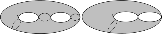
Figure 1: a typical curve and a pinched curve

We conclude this subsection with a comment that deformations with some of the $\mathcal{O}_{n}$’s may give no changes to the algebraic curves. In fact, within our formulation, we can prove (see Appendix C) that any finite perturbation of $\mathcal{O}_{np}\ (n\in\mathbb{N})$ can be absorbed by shifts of $Q$. So we can always take $a_{1}(\zeta)\equiv 0$ with no need to redefine any other backgrounds. In contrast to these, there exist certain combination of $\mathcal{O}_{n}$’s whose infinitesimal perturbation can be absorbed by a shift of $\zeta$. For example, the shift $\zeta\to\zeta-p\,b_{q}/(p+q)b_{p+q}$ makes $b_{q}=0$ without changing the curve, but this induces deformations of other backgrounds parameters (see also [34, 8]).

3.4 A few examples

Here we demonstrate how the above arguments are applied in solving disk amplitudes (especially in fixing the parameters).

1. A nontrivial example: $(p,q)=(3,5)$

We first consider the $(p,q)=(3,5)$ critical point. We set the background to the conformal one; $\tilde{b}_{8}\equiv 8b_{8}/3\equiv 4^{1/3}\beta,\,\tilde{b}_{2}\equiv 2b_{2}/3\equiv-5\beta/(3\cdot 4^{2/3})\cdot\mu$ and otherwise $b_{n}=0$ ($\beta$: a numerical constant). Then $a_{s}(\zeta)$ are calculated to be

$$a_{1}(\zeta) =0,\qquad\quad a_{2}(\zeta)=\tilde{b}_{8}v_{2}\equiv\tilde{v}_{2},$$

$$a_{3}(\zeta) =\tilde{b}_{8}^{3}\,\zeta^{5}+3\,\tilde{b}_{8}^{2}\tilde{b}_{2}\,\zeta^{3}+\tilde{b}_{8}^{2}v_{1}\,\zeta^{2}+(\tilde{b}_{8}^{2}v_{4}+\tilde{b}_{8}\tilde{b}_{2}^{2}\bigr{)}\,\zeta+\tilde{b}_{8}^{2}v_{7}$$

$$\equiv 4\zeta^{5}-5\mu\,\zeta^{3}+\tilde{v}_{1}\,\zeta^{2}+\tilde{v}_{4}\,\zeta+\tilde{v}_{7},$$ (252)

where the parameters $\tilde{v}_{n(s,l)}\,(=\tilde{b}_{8}^{s-1}v_{n(s,l)}+\cdots)$ form the $A$-cycle moduli of the curve with dimensionality $(p-1)(q-1)/2=4$. We now require the existence of the uniformization parameter $z$ on $\mathbb{C}\mathbb{P}^{1}$ [see (243)].

In general, the algebraic equation $F(P(z),Q(z))\equiv 0$ gives relations between $\{b,v\}$ and $\{u\}$, so that $v$ can be solved in $b$ through $u$; $v=v(u(b))$. In this example, the algebraic equation leads to the following solution:

$$P(z) =z^{3}-\frac{3}{4^{1/3}}\mu^{1/3}z^{1}\,\bigl{(}=\zeta\bigr{)}$$ (253)

$$Q(z) =\beta\Bigl{(}4^{1/3}z^{5}-5\mu^{1/3}z^{3}+\frac{5}{4^{1/3}}\mu^{2/3}z\Bigr{)}$$ (254)

$$F(\zeta,Q) =Q^{3}-\frac{3\beta^{2}}{4}\mu^{5/3}Q-\beta^{3}\Bigl{(}4\zeta^{5}-5\mu\zeta^{3}+\frac{5}{4}\mu^{2}\zeta\Bigr{)}$$

$$=\frac{\beta^{3}\mu^{5/2}}{4}\,\bigl{[}\,T_{3}\bigl{(}Q/\mu^{5/6}\bigr{)}-T_{5}\bigl{(}\zeta/\sqrt{\mu}\bigr{)}\,\bigr{]}.$$ (255)

Here $T_{n}(z)$ $(n=0,1,2,\cdots)$ are the first Tchebycheff polynomials of degree $n$, $T_{n}(\cos\tau)\equiv\cos n\tau$, and the algebraic equation gives a solution

$$Q_{0}(\zeta)=\frac{\beta}{2}\left[\Bigl{(}\zeta+\sqrt{\zeta-\sqrt{\mu}}\Bigr{)}^{5/3}+\Bigl{(}\zeta-\sqrt{\zeta-\sqrt{\mu}}\Bigr{)}^{5/3}\right].$$ (256)

2. Kazakov series $(p,q)=(2,2k-1)$

In the case of $(p,q)=(2,2k-1)$, the algebraic equation is written as

$$F(\zeta,Q) =Q^{2}-a_{2}(\zeta)=0,$$ (257)

where the order of $a_{2}(\zeta)$ is $2k-1$. Here we have set $a_{1}(\zeta)=0$ that comes from the backgrounds for $\{\mathcal{O}_{np}\}$ $(n=1,2,\cdots)$. As is shown in Appendix C, $a_{1}(\zeta)$ can be easily recovered by adding $a_{1}(\zeta)/2$ to $Q_{0}(\zeta)$.

The boundary conditions are satisfied if this curve has $k-1$ singularities (251), or equivalently, if the function $a_{2}(\zeta)$ has $k-1$ solutions $\zeta_{*}^{(i)}$ with $a_{2}(\zeta_{*}^{(i)})=a_{2}^{\prime}(\zeta_{*}^{(i)})=0\ (i=1,\cdots k-1)$. The latter conditions are nothing but the so-called one-cut boundary condition, and thus the general solution is given by

$$Q_{0}(\zeta)=\frac{a_{1}(\zeta)}{2}+c\sqrt{\zeta-u}\,\prod_{i=1}^{k-1}\left(\zeta-\zeta_{*}^{(i)}\right).$$ (258)

The corresponding background parameters can be read from

$$b_{m}=\frac{1}{2m}\oint\bigcirc\frac{d\zeta}{2\pi i}\zeta^{-m/2}Q(\zeta),$$ (259)

and all solutions are obtained. The uniformization mapping is given by

$$\zeta=P(z)=z^{2}+u,\qquad Q_{0}=Q(z)=Q_{0}(\zeta(z)).$$ (260)

3. conformal backgrounds

We now consider $(p,q)$ minimal strings in the conformal backgrounds, for which the disk amplitudes are known to be

$$Q_{0}(\zeta)=\frac{\beta}{2}\,\left[\bigl{(}\zeta+\sqrt{\zeta^{2}-\mu}\bigr{)}^{q/p}+\bigl{(}\zeta-\sqrt{\zeta^{2}-\mu}\bigr{)}^{q/p}\right]\quad(\beta:~{}\hbox{numerical~{}constant}).$$ (261)

Expanding this as in (239), we find that the conformal backgrounds should be expressed by the following background parameters:

$$b_{n}=\begin{cases}\displaystyle-\beta\,\frac{p\,q}{n}\,\frac{2^{(q-p)/p}}{2mp-q}\binom{2m-q/p}{m}\left(\frac{\mu}{4}\right)^{m}&\biggl{(}n=q+p-2mp\,;~{}0\leq m\leq\Bigl{[}\dfrac{q+p-1}{2p}\Bigr{]}\biggr{)}\\ 0&\bigl{(}\hbox{otherwise}\bigr{)}\end{cases}.$$ (262)

With this background, as is done in the first example, one can show that the requirement of maximal degeneracy leads the polynomials $a_{s}(\zeta)$ to have the following values:

$$s\,a_{s}(\zeta)=\delta_{s,p}\,2p\left(\frac{\beta\mu^{q/2p}}{2}\right)^{p}T_{q}\bigl{(}\zeta/\sqrt{\mu}\bigr{)}+\begin{cases}\displaystyle p\left(\frac{\beta\mu^{q/2p}}{2}\right)^{s}\binom{s}{s/2}&(s\text{: even})\\ 0&(s\text{: odd})\end{cases}.$$ (263)

To calculate the corresponding algebraic equation $F(\zeta,Q)=0$, in this case it turns out to be useful to write it as follows:

$$F(\zeta,Q) =Q^{p}\exp\big{(}-\sum_{n=1}^{\infty}a_{n}(\zeta)\,Q^{-n}\big{)}\equiv Q^{p}\exp G(\zeta,Q)$$

$$=\big{[}Q^{p}\exp\big{\{}G(\zeta,Q)+O\big{(}Q^{-p-1}\big{)}\big{\}}\big{]}_{{\rm pol}}.$$ (264)

In fact, the explicit form of the function $G(\zeta,Q)$ is given by

$$G(\zeta,Q)=p\log\left(\frac{1+\sqrt{1-\beta^{2}\mu^{q/p}Q^{-2}}}{2}\right)-2\left(\frac{\beta\mu^{q/2p}}{2Q}\right)^{p}T_{q}\bigl{(}\zeta/\mu\bigr{)}+O(Q^{-p-1}),$$ (265)

and with the knowledge that $F(\zeta,Q)$ is a polynomial both of $\zeta$ and $Q$, we obtain the following algebraic equation:

$$F(\zeta,Q)=2\left(\frac{\beta\mu^{q/2p}}{2}\right)^{p}\bigl{[}\,T_{p}\bigl{(}Q/\beta\mu^{q/2p}\bigr{)}-T_{q}\bigl{(}\zeta/\sqrt{\mu}\bigr{)}\,\bigr{]}=0.$$ (266)

This can be solved as

$$P(z)=\zeta=\sqrt{\mu}\,T_{p}(z),\qquad Q(z)=Q_{0}=\beta\,\mu^{q/2p}\,T_{q}(z),$$ (267)

with the uniformization parameter $z\in\mathbb{C}\mathbb{P}^{1}$. This agrees with the result found in Liouville theory [8].

4 Amplitudes of FZZT branes II - annulus amplitudes

We now consider the annulus amplitudes and show that they can be calculated in two ways. One is using the structure of the KP hierarchy alone. The other is using the $W_{1+\infty}$ constraints with requiring the uniformizing parameter to live on $\mathbb{C}\mathbb{P}^{1}$.

4.1 Annulus amplitudes from the KP hierarchy

The main aim of this subsection is to prove the following theorem:

Theorem 6.

For any backgrounds, the annulus amplitudes are always given by

$$\left\langle\partial\varphi_{0}(\zeta_{1})\partial\varphi_{0}(\zeta_{2})\right\rangle_{\rm c}^{\!(0)}=\partial_{\zeta_{1}}\partial_{\zeta_{2}}\ln\left(\frac{z_{1}-z_{2}}{\zeta_{1}-\zeta_{2}}\right)$$ (268)

with the uniformization mapping $\zeta=\zeta(z)$ given in (243).

From this theorem, we see that the annulus amplitudes depend only on the uniformization mapping $\zeta=\zeta(z)=\bigl{(}\lambda(z)\bigr{)}^{p}$ associated with the Lax operator $\bm{L}=\partial+\sum_{n=2}^{\infty}u_{n}\partial^{-n+1}$. In other words, the structure of the annulus amplitudes is totally determined by that of the KP hierarchy, and the dynamics enters only through the uniformization mapping. Note that for the conformal backgrounds, the uniformization parameter $z$ is given by (267), $\zeta(z)=\sqrt{\mu}\,T_{p}(z)$, and thus the annulus amplitudes found in [38, 11] are correctly reproduced:

$$\left\langle\partial\varphi_{0}(\zeta_{1})\partial\varphi_{0}(\zeta_{2})\right\rangle_{\rm c}^{\!(0)}=\partial_{\zeta_{1}}\partial_{\zeta_{2}}\ln\left(\frac{z_{1}-z_{2}}{T_{p}(z_{1})-T_{p}(z_{2})}\right).$$ (269)

To prove the theorem we first show:

Lemma 2.

For the weak coupling limit of the Lax operator, $L(x,z)=\lambda=z\,\bigl{(}1+\sum_{n=2}^{\infty}u_{n}(x)\,z^{-n}\bigr{)}$, the following relation holds:

$$\left[\lambda^{n}\right]_{-}(z)=\sum_{m=1}^{\infty}\frac{v_{nm}}{m}\,\lambda^{-m}\quad(n\geq 1).$$ (270)

Here $[~{}~{}]_{-}(z)$ denotes the negative-power part in $z$, and $v_{nm}\equiv\left\langle\mathcal{O}_{n}\mathcal{O}_{m}\right\rangle^{\!(0)}_{\rm c}$.

Proof of the lemma. In the weak coupling limit, the Baker-Akhiezer function is approximated as

$$\Psi(x;\lambda) =\frac{\bigl{<}x\bigr{|}e^{\phi_{+}(\lambda)}\bigl{|}\Phi\bigr{>}}{\left.\left\langle x\right|\Phi\right\rangle}\exp\big{[}g^{-1}\sum_{n=1}^{\infty}x_{n}\lambda^{n}\big{]}$$

$$=\exp\Bigl{[}g^{-1}\Bigl{(}\left\langle\phi_{+}(\lambda)\right\rangle^{(0)}+\sum_{n=1}^{\infty}x_{n}\lambda^{n}\Bigr{)}+O(g^{0})\Bigr{]}$$

$$=\exp\Big{[}g^{-1}\Bigl{(}-\sum_{m=1}^{\infty}\frac{v_{m}}{m}\lambda^{-m}+\sum_{n=1}^{\infty}x_{n}\lambda^{n}\Bigr{)}+O(g^{0})\Big{]},$$ (271)

and thus we obtain

$$\frac{\partial\Psi}{\partial x_{n}}=\frac{1}{g}\,(\lambda^{n}-\sum_{m=1}^{\infty}\frac{v_{nm}}{m}\lambda^{-m})\Psi+O(g^{0}).$$ (272)

The left-hand side can also be calculated by using the linear problem of the KP hierarchy as

$$\frac{\partial\Psi}{\partial x_{n}}=\frac{1}{g}\,(\bm{L}^{n})_{+}\Psi=\frac{1}{g}\,\bigl{(}\lambda^{n}-[\lambda^{n}]_{-}(z)\bigr{)}\Psi.$$ (273)

Comparing (272) and (273), we obtain

$$\left[\lambda^{n}\right]_{-}(z)=\sum_{m=1}^{\infty}\frac{v_{nm}}{m}\,\lambda^{-m}.\qquad\Box$$ (274)

Proof of the theorem. We recall that the annulus amplitudes $\left\langle\partial\varphi_{0}(\zeta_{1})\,\partial\varphi_{0}(\zeta_{2})\right\rangle_{\rm c}^{\!(0)}$ are written as

$$\left\langle\partial\varphi_{0}(\zeta_{1})\,\partial\varphi_{0}(\zeta_{2})\right\rangle_{\rm c}^{\!(0)} =\left\langle\partial\varphi_{0,+}(\zeta_{1})\partial\varphi_{0,+}(\zeta_{2})\right\rangle_{\rm c}^{\!(0)}+\frac{d\lambda_{1}}{d\zeta_{1}}\frac{d\lambda_{2}}{d\zeta_{2}}\frac{1}{(\lambda_{1}-\lambda_{2})^{2}}-\frac{1}{(\zeta_{1}-\zeta_{2})^{2}}$$

$$=\frac{d\lambda_{1}}{d\zeta_{1}}\frac{d\lambda_{2}}{d\zeta_{2}}\left(\left\langle\partial\phi_{+}(\lambda_{1})\partial\phi_{+}(\lambda_{2})\right\rangle_{\rm c}^{\!(0)}+\frac{1}{(\lambda_{1}-\lambda_{2})^{2}}\right)-\frac{1}{(\zeta_{1}-\zeta_{2})^{2}},$$ (275)

so that it is sufficient to show the identity

$$\left\langle\partial\phi_{+}(\lambda_{1})\,\phi_{+}(\lambda_{2})\right\rangle_{\rm c}^{\!(0)}=\partial_{\lambda_{1}}\ln\frac{z_{1}-z_{2}}{\lambda_{1}-\lambda_{2}}\quad(|\lambda_{1}|>|\lambda_{2}|).$$ (276)

We prove this for a region where $|\zeta_{1}|$ is sufficiently larger than $|\zeta_{2}|$, so that we can assume $|\lambda_{1}|>|\lambda_{2}|$ and $|z_{1}|>|z_{2}|$. Once the statement holds in this region, it should also hold in other regions. Then,

$$\left\langle\partial\phi_{+}(\lambda_{1})\,\phi_{+}(\lambda_{2})\right\rangle_{\rm c}^{\!(0)} =-\sum_{n,m\geq 1}\frac{v_{nm}}{m}\lambda_{1}^{-n-1}\lambda_{2}^{-m}=-\sum_{n\geq 1}\lambda_{1}^{-n-1}[\lambda^{n}(z_{2})]_{-}(z_{2})$$

$$=\sum_{n\geq 1}\lambda_{1}^{-n-1}\oint_{|z|<|z_{2}|<|z_{1}|}\!\frac{dz}{2\pi i}\,\frac{\lambda^{n}(z)}{z-z_{2}}$$

$$=\oint_{|z|<|z_{2}|<|z_{1}|}\!\frac{dz}{2\pi i}\,\frac{1}{z-z_{2}}\ \frac{1}{\lambda_{1}-\lambda(z)}$$

$$=-\Bigl{(}\oint_{z_{1}}+\oint_{z_{2}}\Bigr{)}\,\frac{dz}{2\pi i}\,\frac{1}{z-z_{2}}\,\frac{1}{\lambda_{1}-\lambda(z)}.$$ (277)

Here we have used the fact that for an arbitrary function with the (formal) Laurent expansion $\displaystyle f(z)=\sum_{n\in\mathbb{Z}}f_{n}\,z^{n}$, its negative-power part has an integral representation as

$$[f(z)]_{-} \equiv\sum_{n\leq-1}f_{n}z^{n}=-\oint_{|x|<|z|}\frac{dx}{2\pi i}\,\frac{f(x)}{x-z}.$$ (278)

Also, to obtain the last line of (277), we have deformed the contour by noting that there is no simple pole at $z=\infty$. Each term in (277) is then evaluated as

$$\oint_{z_{1}}\frac{dz}{2\pi i}\,\frac{1}{z-z_{2}}\ \frac{1}{\lambda_{1}-\lambda(z)} =\oint_{\lambda_{1}}\frac{d\lambda}{2\pi i}\,\frac{dz}{d\lambda}\,\frac{1}{z-z_{2}}\,\frac{1}{\lambda_{1}-\lambda}$$

$$=-\frac{dz_{1}}{d\lambda_{1}}\ \frac{1}{z_{1}-z_{2}}=-\partial_{\lambda_{1}}\ln(z_{1}-z_{2}),$$ (279)

$$\oint_{z_{2}}\frac{dz}{2\pi i}\,\frac{1}{z-z_{2}}\ \frac{1}{\lambda_{1}-\lambda(z)} =\frac{1}{\lambda_{1}-\lambda_{2}}=\partial_{\lambda_{1}}\ln(\lambda_{1}-\lambda_{2}),$$ (280)

and thus we obtain (276). $\qquad\Box$

4.2 Annulus amplitudes for FZZT branes

Integrating (268) we obtain the annulus amplitudes for FZZT branes in general backgrounds $b=(b_{n})$:

$$\left\langle\,\varphi_{0}(\zeta_{1})\,\varphi_{0}(\zeta_{2}\,)\right\rangle_{\rm c}^{\!(0)}=\ln\left(\frac{z_{1}-z_{2}}{\zeta_{1}-\zeta_{2}}\right).$$ (281)

We here make a comment that $\left\langle\varphi_{a}(\zeta_{1})\varphi_{b}(\zeta_{2})\right\rangle$ does not obey simple monodromy [2, 4]. This is due to the fact that the two-point function $\left\langle\varphi_{a}(\zeta_{1})\varphi_{b}(\zeta_{2})\right\rangle$ is defined with the normal ordering $:\ \ :$ that respects the $\mathop{\rm SL}(2,\mathbb{C})$ invariance on the $\lambda$ plane:

$$\left\langle\varphi_{a}(\zeta_{1})\varphi_{b}(\zeta_{2})\right\rangle =\frac{\left\langle b/g|:\!\varphi_{a}(\zeta_{1})\varphi_{b}(\zeta_{2})\!:|\Phi\right\rangle}{\left\langle b/g|\Phi\right\rangle}.$$ (282)

In fact, by using the definition $:\!\varphi_{a}(\zeta_{1})\,\varphi_{b}(\zeta_{2})\!:\,=\varphi_{a}(\zeta_{1})\,\varphi_{b}(\zeta_{2})-\delta_{ab}\,\ln(\zeta_{1}-\zeta_{2})$, the two-point functions are expressed as

$$\left\langle\,\varphi_{a}(\zeta_{1})\,\varphi_{b}(\zeta_{2})\,\right\rangle =\frac{\left\langle b/g|\,\varphi_{a}(\zeta_{1})\varphi_{b}(\zeta_{2})\,|\Phi\right\rangle}{\left\langle b/g|\Phi\right\rangle}-\delta_{ab}\ln(\zeta_{1}-\zeta_{2})$$

$$=\frac{\left\langle b/g|\,\varphi_{0}(e^{2\pi ia}\zeta_{1})\varphi_{0}(e^{2\pi ib}\zeta_{2})\,|\Phi\right\rangle}{\left\langle b/g|\Phi\right\rangle}-\delta_{ab}\ln(\zeta_{1}-\zeta_{2})$$

$$=\frac{\left\langle b/g|:\!\varphi_{0}(e^{2\pi ia}\zeta_{1})\varphi_{0}(e^{2\pi ib}\zeta_{2})\!:|\Phi\right\rangle}{\left\langle b/g|\Phi\right\rangle}+$$

$$~{}~{}~{}~{}~{}~{}~{}+\ln(e^{2\pi ia}\zeta_{1}-e^{2\pi ib}\zeta_{2})-\delta_{ab}\ln(\zeta_{1}-\zeta_{2})$$

$$=\left\langle\varphi_{0}(e^{2\pi ia}\zeta_{1})\,\varphi_{0}(e^{2\pi ib}\zeta_{2})\right\rangle+\ln(e^{2\pi ia}\zeta_{1}-e^{2\pi ib}\zeta_{2})-\delta_{ab}\ln(\zeta_{1}-\zeta_{2}).$$ (283)

We thus obtain

$$\left\langle\,\varphi_{a}(\zeta_{1})\,\varphi_{b}(\zeta_{2}\,)\right\rangle_{\rm c}^{\!(0)}=\ln\bigl{(}z_{1a}-z_{2b}\bigr{)}-\delta_{ab}\ln\bigl{(}\zeta_{1}-\zeta_{2}\bigr{)},$$ (284)

where $z_{a}$ is the inverse of $e^{2\pi ia}\zeta$ under the mapping $\zeta=\zeta(z)$.

For the conformal backgrounds (262), the annulus amplitudes become

$$\langle\varphi_{a}(\zeta_{1})\varphi_{b}(\zeta_{2})\rangle_{\rm c}^{\!(0)}=\ln\bigl{(}z_{1a}-z_{2b}\bigr{)}-\delta_{ab}\ln\bigl{[}\sqrt{\mu}\bigl{(}T_{p}(z_{1})-T_{p}(z_{2})\bigr{)}\bigr{]}.$$ (285)

The $K_{ab}(z)$ in (213) can be calculated easily and are found to be

$$K_{ab}(z) =-\ln\left[-U_{p-1}(z_{a})U_{p-1}(z_{b})(z_{a}-z_{b})^{2}\right]-2\ln p\sqrt{\mu}.$$ (286)

Here $U_{n}(z)$ $(n=0,1,2,\cdots)$ are the second Tchebycheff polynomials of degree $n$ defined by $U_{n}(\cos\tau)\equiv\sin(n+1)\tau/\sin\tau$, and $z_{a}$ in this case can be written as $z_{a}\equiv\cos\tau_{a}\equiv\cos(\tau+2\pi a/p)$ with $z=\cos\tau$ and $\zeta=\sqrt{\mu}\,T_{p}(z)$.

4.3 Schwinger-Dyson equations for annulus amplitudes

In this and subsequent subsections, we show that the annulus amplitudes can also be investigated from the approach based on the Schwinger-Dyson equations. We first derive the equations by imposing the $W_{1+\infty}$ constraints on the function

$$\left\langle\left\langle W^{s}(\zeta_{1})W^{t}(\zeta_{2})\right\rangle\right\rangle_{\rm c}\equiv\left\langle\left\langle W^{s}(\zeta_{1})W^{t}(\zeta_{2})\right\rangle\right\rangle-\left\langle W^{s}(\zeta_{1})\right\rangle\,\left\langle W^{t}(\zeta_{2})\right\rangle.$$ (287)

We then investigate the structure of the Schwinger-Dyson equations and demonstrate how they are solved. We will find that the Schwinger-Dyson equations again have undetermined constants, and see that they are completely fixed upon demanding the existence of the uniformizing parameter $z$ on $\mathbb{C}\mathbb{P}^{1}$, as is the case for disk amplitudes. Proofs of some of the statements made in this subsection are collected in Appendix D.

We first note:

Proposition 4.

The weak coupling limit of the expectation value $\left\langle\left\langle W^{s}(\zeta_{1})W^{t}(\zeta_{2})\right\rangle\right\rangle_{\rm c}$ is given by

$$\left\langle\left\langle W^{s}(\zeta_{1})W^{t}(\zeta_{2})\right\rangle\right\rangle_{\rm c} \equiv\frac{st}{g^{s+t-2}}\sum_{a,b=0}^{p-1}Q_{a}^{s-1}(\zeta_{1})\,A_{ab}(\zeta_{1},\zeta_{2})\,Q_{b}^{t-1}(\zeta_{2})+O(g^{-s-t+3})$$

$$=\frac{st}{g^{s+t-2}}\cdot p^{2}\,\bigl{[}Q_{0}^{s-1}(\zeta_{1})\,A_{00}(\zeta_{1},\zeta_{2})\,Q_{0}^{t-1}(\zeta_{2})\bigr{]}_{{\rm int}}+O(g^{-s-t+3})$$ (288)

with

$$A_{ab}(\zeta_{1},\zeta_{2})\equiv\left\langle\partial\varphi_{a}(\zeta_{1})\partial\varphi_{b}(\zeta_{2})\right\rangle^{\!(0)}_{\rm c}+\frac{\delta_{ab}}{(\zeta_{1}-\zeta_{2})^{2}}.$$ (289)

Here, the integer-power part of a function $\displaystyle f(\zeta_{1},\zeta_{2})=\sum_{m,n\in\mathbb{Z}}f_{m,n}\,\zeta_{1}^{m/p}\zeta_{2}^{n/p}$ is denoted by $\displaystyle\bigl{[}f(\zeta_{1},\zeta_{2})\bigr{]}_{{\rm int}}\equiv\sum_{k,l\in\mathbb{Z}}f_{kp,lp}\,\zeta_{1}^{k}\,\zeta_{2}^{l}$.

Since $\left\langle\left\langle W^{s}(\zeta_{1})W^{t}(\zeta_{2})\right\rangle\right\rangle_{\rm c}$ is defined with the radial ordering, we need a care in imposing the $W_{1+\infty}$ constraints (150) on the function. We thus consider two regions in $(\zeta_{1},\zeta_{2})$ separately: (I) $|\zeta_{1}|>|\zeta_{2}|$ and (II) $|\zeta_{2}|>|\zeta_{1}|$, and make a double series expansion in each case. With this consideration, one obtains the following proposition:

Proposition 5.

By expanding $\displaystyle\left\langle\left\langle W^{s}(\zeta_{1})W^{t}(\zeta_{2})\right\rangle\right\rangle_{\rm c}$ as $\sum_{M,N\in\mathbb{Z}}W^{s,t\,(i)}_{M,N}\,\zeta_{1}^{M}\zeta_{2}^{N}$ (for the region $i={\rm I,II}$), the coefficients $W^{s,t\,(i)}_{M,N}$ satisfy the following conditions:

$$\text{{\rm(W1)}\quad$W^{s,t\,({\rm I})}_{M,N}=0$ unless $N\geq 0$ and $M+N\geq-2$},$$ (290)

$$\text{{\rm(W2)}\quad$W^{s,t\,({\rm II})}_{M,N}=0$ unless $M\geq 0$ and $M+N\geq-2$}.$$ (291)

These conditions are also sufficient for reproducing the $W_{1+\infty}$ constraints.

We denote by $\bigl{[}f(\zeta_{1},\zeta_{2})\bigr{]}_{W}$ the part of a function $f(\zeta_{1},\zeta_{2})$ that satisfies both of (W1) and (W2) of Proposition 5. Then we can write the Schwinger-Dyson equations for annulus amplitudes in the following way:

$$\sum_{a,b=0}^{p-1}Q_{a}^{s-1}(\zeta_{1})A_{ab}(\zeta_{1},\zeta_{2})Q_{b}^{t-1}(\zeta_{2})=p^{2}\big{[}Q_{0}^{s-1}(\zeta_{1})A_{00}(\zeta_{1},\zeta_{2})Q_{0}^{t-1}(\zeta_{2})\big{]}_{W}\equiv G_{st}(\zeta_{1},\zeta_{2}).$$ (292)

We can solve this set of equations for $A_{ab}(\zeta_{1},\zeta_{2})$, by using the fact that the inverse of the matrix $(X^{s}{}_{a})=(Q^{s-1}_{a}(\zeta))_{a=0,\cdots,p-1}^{s=1,\cdots,p}$ is given by

$$(X^{-1})^{a}{}_{s}=\frac{\Delta^{(a)}(Q(\zeta))}{\Delta(Q(\zeta))}(-1)^{a+s}\sigma_{p-s}^{(a)}(\zeta),$$ (293)

where $\sigma^{(a)}_{n}(\zeta)$ and $\Delta^{(a)}(Q)$ are, respectively, the elementary symmetric functions and Van der Monde determinant of $\{Q_{b}\}_{b=0,\neq a}^{p-1}$:

$$\sigma^{(a)}_{n}(\zeta)=\sum_{0\leq a_{1}<\cdots<a_{n}\leq p-1,\,a_{i}\neq a}Q_{a_{1}}(\zeta)\cdots Q_{a_{n}}(\zeta),\qquad\Delta^{(a)}(Q)=\det\big{[}(Q_{i-1}^{j-1})_{i,j=1,i\neq a,j\neq p}^{p}\big{]}.$$ (294)

We thus obtain:

Theorem 7.

The Schwinger-Dyson equations for the annulus amplitudes are solved as

$$\left\langle\partial\varphi_{a}(\zeta_{1})\,\partial\varphi_{b}(\zeta_{2})\right\rangle_{\rm c}^{\!(0)}=A_{ab}(\zeta_{1},\zeta_{2})-\frac{\delta_{ab}}{(\zeta_{1}-\zeta_{2})^{2}}$$ (295)

with

$$A_{ab}(\zeta_{1},\zeta_{2})=\frac{\Delta^{(a)}(Q(\zeta_{1}))\,\Delta^{(b)}(Q(\zeta_{2}))}{\Delta(Q(\zeta_{1}))\,\Delta(Q(\zeta_{2}))}\sum_{s,t=1}^{p}(-1)^{a+b+s+t}\,\sigma^{(a)}_{p-s}(\zeta_{1})\,\sigma^{(b)}_{p-t}(\zeta_{2})\,G_{st}(\zeta_{1},\zeta_{2}).$$ (296)

4.4 Structure of the Schwinger-Dyson equations for annulus amplitudes

We next investigate the structure of the function $G_{st}(\zeta_{1},\zeta_{2})$ defined in (292). From the equation (188), one can see that $A_{ab}(\zeta_{1},\zeta_{2})$ has the following double series expansion:

$$A_{00}(\zeta_{1},\zeta_{2}) =\frac{d\zeta_{1}^{1/p}}{d\zeta_{1}}\frac{d\zeta_{2}^{1/p}}{d\zeta_{2}}\frac{1}{(\zeta_{1}^{1/p}-\zeta_{2}^{1/p})^{2}}+\frac{1}{p^{2}}\sum_{n,m\in\mathbb{Z}}v_{nm}\,\zeta_{1}^{-n/p-1}\zeta_{2}^{-m/p-1}$$

$$\equiv\widetilde{N}+\widetilde{A},$$ (297)

where the first term (part of the nonuniversal terms) is denoted by $\widetilde{N}$ and the second term (universal terms) by $\widetilde{A}$, and $v_{nm}\equiv\left\langle\mathcal{O}_{n}\mathcal{O}_{m}\right\rangle_{\rm c}^{\!(0)}$. Accordingly, $G_{st}(\zeta_{1},\zeta_{2})$ is decomposed as

$$G_{st}(\zeta_{1},\zeta_{2})=p^{2}\big{[}Q_{0}^{s-1}(\zeta_{1})(\widetilde{N}+\widetilde{A})Q_{0}^{t-1}(\zeta_{2})\big{]}_{W}\equiv G_{st}^{N}(\zeta_{1},\zeta_{2})+G_{st}^{A}(\zeta_{1},\zeta_{2}).$$ (298)

We first consider $G_{st}^{N}(\zeta_{1},\zeta_{2})\equiv p^{2}\big{[}Q_{0}^{s-1}(\zeta_{1})\widetilde{N}(\zeta_{1},\zeta_{2})Q_{0}^{t-1}(\zeta_{2})\big{]}_{W}$. It turns out to be convenient to decompose the disk amplitudes $Q_{a}(\zeta)$ into the parts diagonal to the $\mathbb{Z}_{p}$ monodromy:

$$Q_{0}^{s-1}(\zeta)\equiv\sum_{b=0}^{p-1}R_{b}^{(s-1)}(\zeta)\equiv\sum_{b=0}^{p-1}\widetilde{R}^{(s-1)}_{b}(\zeta)\zeta^{-b/p+1},$$ (299)

where $\widetilde{R}^{(s-1)}_{b}(\zeta)\equiv[\zeta^{b/p-1}Q_{0}^{s-1}]_{{\rm int}}$, and $R_{b}^{(s-1)}(\zeta)\equiv\widetilde{R}^{(s-1)}_{b}(\zeta)\zeta^{-b/p+1}$ has the monodromy $R_{b}^{(s-1)}(e^{2\pi i}\zeta)=\omega^{-b}R_{b}^{(s-1)}(\zeta)$. We thus obtain

$$G_{st}^{N}(\zeta_{1},\zeta_{2})=\Bigl{[}\sum_{r=0}^{p-1}\widetilde{R}^{(s-1)}_{p-r}(\zeta_{1})\widetilde{R}^{(t-1)}_{r}(\zeta_{2})\frac{(p-r)\zeta_{2}+r\zeta_{1}}{(\zeta_{1}-\zeta_{2})^{2}}\Bigr{]}_{W}.$$ (300)

We can easily see that under the conditions (W1) and (W2) only finite terms survive in the double series expansion. In fact, each of the terms can be rewritten by using the following formula:

$$\Bigl{[}j(\zeta_{1})\bigg{(}\frac{\zeta_{1}}{\zeta_{2}}\bigg{)}^{n}\frac{1}{(\zeta_{1}-\zeta_{2})^{2}}\Bigr{]}_{W}=\Bigl{[}\frac{j(\zeta_{1})}{(\zeta_{1}-\zeta_{2})^{2}}+n\,\frac{j(\zeta_{1})}{\zeta_{1}(\zeta_{1}-\zeta_{2})}\Bigr{]}_{W}$$ (301)

with an arbitrary polynomial $j(\zeta_{1})$, as well as the ones with $\zeta_{1}\leftrightarrow\zeta_{2}$. Furthermore, if we reach the following expression after repeatedly using the above formula:

$$\cdots=\Bigl{[}\frac{h(\zeta_{1},\zeta_{2})}{(\zeta_{1}-\zeta_{2})^{2}}\Bigr{]}_{W}$$ (302)

with $h(\zeta_{1},\zeta_{2})$ an arbitrary polynomial in $\zeta_{1}$ and $\zeta_{2}$, then $[\ ]_{W}$ can be taken off from the expression,

$$\Bigl{[}\frac{h(\zeta_{1},\zeta_{2})}{(\zeta_{1}-\zeta_{2})^{2}}\Bigr{]}_{W}=\frac{h(\zeta_{1},\zeta_{2})}{(\zeta_{1}-\zeta_{2})^{2}},$$ (303)

since the inside already satisfies both of the conditions (W1) and (W2), as one can easily show. This consideration leads to:

Proposition 6.

For any pair of functions of the form $\displaystyle f(\zeta)=\sum_{n=-\infty}^{\infty}a_{n}\zeta^{n}$ and $\displaystyle g(\zeta)=\sum_{n=-\infty}^{-1}b_{n}\zeta^{n}$, the following identity holds under the $W_{1+\infty}$ constraints:

$$\Bigl{[}\frac{f(\zeta_{1})g(\zeta_{2})}{(\zeta_{1}-\zeta_{2})^{2}}\Bigr{]}_{W}=\frac{\bigl{[}f(\zeta_{1})g(\zeta_{1})\bigr{]}_{{\rm pol}}}{(\zeta_{1}-\zeta_{2})^{2}}-\frac{\bigl{[}f(\zeta_{1})\partial g(\zeta_{1})\bigr{]}_{{\rm pol}}}{(\zeta_{1}-\zeta_{2})}-\Bigl{[}\frac{[f(\zeta_{1})\partial g(\zeta_{1})]_{-1}}{\zeta_{1}(\zeta_{1}-\zeta_{2})}\Bigr{]}_{W},$$ (304)

where $[f]_{-1}$ denotes the coefficient of $\zeta^{-1}$ in $f(\zeta)$.

Note that the last term in eq. (304) (i.e. $1/\zeta_{1}(\zeta_{1}-\zeta_{2})$) does not satisfy (W1) and (W2) simultaneously, but the contributions from such terms totally disappear in the final results and thus can be ignored.

Repeatedly using the proposition, we obtain:

Proposition 7.

The function $G_{st}^{N}(\zeta_{1},\zeta_{2})$ can be written as

$$G_{st}^{N} =\frac{1}{(\zeta_{1}-\zeta_{2})^{2}}\Bigl{(}\frac{(s-1)(t-1)}{p}a_{s-1}(\zeta_{1})a_{t-1}(\zeta_{2})+B_{st,0}(\zeta_{1},\zeta_{2})+B_{st,1}(\zeta_{1})+B_{st,2}(\zeta_{2})-$$

$$\qquad\qquad\qquad\qquad\qquad-(\zeta_{1}-\zeta_{2})(B_{st,3}(\zeta_{1})-B_{st,4}(\zeta_{2}))\Bigr{)}$$

$$\equiv\frac{1}{(\zeta_{1}-\zeta_{2})^{2}}\Bigl{(}\frac{(s-1)(t-1)}{p}a_{s-1}(\zeta_{1})a_{t-1}(\zeta_{2})+B_{st}^{N}(\zeta_{1},\zeta_{2})\Bigr{)},$$ (305)

where

$$B_{st,0}(\zeta_{1},\zeta_{2}) \equiv\sum_{r=1}^{p-r}\Bigl{(}(p-r)\,[\zeta_{1}^{-r/p}Q_{0}^{s-1}(\zeta_{1})]_{{\rm pol}}\,[\zeta_{2}^{r/p}Q^{t-1}_{0}(\zeta_{2})]_{{\rm pol}}+$$

$$\qquad\qquad\qquad+r\,[\zeta_{1}^{(p-r)/p}Q^{s-1}_{0}(\zeta_{1})]_{{\rm pol}}\,[\zeta_{2}^{-(p-r)/p}Q^{t-1}_{0}(\zeta_{2})]_{{\rm pol}}\Bigr{)},$$ (306)

$$B_{st,1}(\zeta_{1}) \equiv\sum_{r=1}^{p-r}\bigg{(}(p-r)\big{[}\zeta_{1}^{-r/p}Q_{0}^{s-1}(\zeta_{1})\,\big{(}\zeta_{1}^{r/p}Q^{t-1}_{0}(\zeta_{1})\big{)}_{-}\big{]}_{{\rm pol}}+$$

$$\qquad\qquad\qquad+r\,\big{[}\zeta_{1}^{(p-r)/p}Q_{0}^{s-1}(\zeta_{1})\,\big{(}\zeta_{1}^{-(p-r)/p}Q^{t-1}_{0}(\zeta_{1})\big{)}_{-}\big{]}_{{\rm pol}}\Bigr{)},$$ (307)

$$B_{st,2}(\zeta_{2}) \equiv\sum_{r=1}^{p-r}\Bigl{(}(p-r)\,\big{[}\big{(}\zeta_{2}^{-r/p}Q_{0}^{s-1}(\zeta_{2})\big{)}_{-}\zeta_{2}^{r/p}Q^{t-1}_{0}(\zeta_{2})\big{]}_{{\rm pol}}+$$

$$\qquad\qquad\qquad+r\,\big{[}\big{(}\zeta_{2}^{(p-r)/p}Q_{0}^{s-1}(\zeta_{2})\big{)}_{-}\zeta_{2}^{-(p-r)/p}Q^{t-1}_{0}(\zeta_{2})\big{]}_{{\rm pol}}\Bigr{)},$$ (308)

$$B_{st,3}(\zeta_{1}) \equiv\sum_{r=1}^{p-r}\Bigl{(}(p-r)\,\big{[}\zeta_{1}^{-r/p}Q_{0}^{s-1}(\zeta_{1})\,\partial\big{(}\zeta_{1}^{r/p}Q^{t-1}_{0}(\zeta_{1})\big{)}_{-}\big{]}_{{\rm pol}}+$$

$$\qquad\qquad\qquad+r\,\big{[}\zeta_{1}^{(p-r)/p}Q_{0}^{s-1}(\zeta_{1})\,\partial\big{(}\zeta_{1}^{-(p-r)/p}Q^{t-1}_{0}(\zeta_{1})\big{)}_{-}\big{]}_{{\rm pol}}\Bigr{)},$$ (309)

$$B_{st,4}(\zeta_{2}) \equiv\sum_{r=1}^{p-r}\,\Bigl{(}(p-r)\big{[}\partial\big{(}\zeta_{2}^{-r/p}Q_{0}^{s-1}(\zeta_{2})\big{)}_{-}\zeta_{2}^{r/p}Q^{t-1}_{0}(\zeta_{2})\big{]}_{{\rm pol}}-$$

$$\qquad\qquad\qquad-r\,\big{[}\partial\big{(}\zeta_{2}^{(p-r)/p}Q_{0}^{s-1}(\zeta_{2})\big{)}_{-}\zeta_{2}^{-(p-r)/p}Q^{t-1}_{0}(\zeta_{2})\big{]}_{{\rm pol}}\Bigr{)},$$ (310)

and $[~{}~{}]_{-}$ denotes the part consisting of negative integer powers.

We next consider $G_{st}^{A}\equiv p^{2}\big{[}Q_{0}^{s-1}(\zeta_{1})\widetilde{A}(\zeta_{1},\zeta_{2})Q_{0}^{t-1}(\zeta_{2})\big{]}_{W}$. With the $W_{1+\infty}$ constraints, this is a polynomial in $\zeta_{1}$ and $\zeta_{2}$, and each coefficient depends on $v_{mn}=\langle O_{m}O_{n}\rangle_{\rm c}^{(0)}$:

$$G_{st}^{A}(\zeta_{1},\zeta_{2}) =\sum_{l_{1}=0}^{[\frac{(s-1)q-1}{p}]-1}\ \sum_{l_{2}=0}^{[\frac{(t-1)q-1}{p}]-1}G_{st,l_{1}l_{2}}^{A}\ \zeta_{1}^{l_{1}}\zeta_{2}^{l_{2}},$$ (311)

$$G_{st,l_{1}l_{2}}^{A} =\frac{st}{p^{s+t-2}}\,[(p+q)b_{p+q}]^{s+t-2}\cdot v_{n(s,l_{1})n(t,l_{2})}+\cdots,$$ (312)

where $n(s,l)$ is given by (248). So this is the counterpart of $a_{s}^{(v)}(\zeta)$ of the disk case, and one can set all the coefficients to arbitrary values by tuning the $v_{nm}$’s. If we denote the number of the moduli of ZZ branes by $N_{ZZ}=(p-1)(q-1)/2$, the total degrees of freedom of $G_{st}^{A}$ is $N_{ZZ}(N_{ZZ}+1)/2$ (i.e. $N_{ZZ}^{2}$ variables with the identification $v_{mn}=v_{nm}$), which is equal to the number that we expect.

By putting everything together, the function $G_{st}(\zeta_{1},\zeta_{2})$ is expressed as

$$G_{st}(\zeta_{1},\zeta_{2}) =G_{st}^{N}(\zeta_{1},\zeta_{2})+G_{st}^{A}(\zeta_{1},\zeta_{2})$$

$$=\frac{1}{(\zeta_{1}-\zeta_{2})^{2}}\Bigl{(}\frac{(s-1)(t-1)}{p}a_{s-1}(\zeta_{1})a_{t-1}(\zeta_{2})+$$

$$\qquad\qquad\qquad\qquad\ \quad+B_{st}^{N}(\zeta_{1},\zeta_{2})+(\zeta_{1}-\zeta_{2})^{2}\,G_{st}^{A}(\zeta_{1},\zeta_{2})\Bigr{)}$$

$$\equiv\frac{1}{(\zeta_{1}-\zeta_{2})^{2}}\Bigl{(}\frac{(s-1)(t-1)}{p}a_{s-1}(\zeta_{1})a_{t-1}(\zeta_{2})+B_{st}(\zeta_{1},\zeta_{2})\Bigr{)},$$ (313)

and by substituting the function $G_{st}(\zeta_{1},\zeta_{2})$ into the inversion formula (296), the annulus amplitudes can be written as

$$A_{ab}(\zeta_{1},\zeta_{2})=\frac{F_{ab}(\zeta_{1},\zeta_{2})}{(\zeta_{1}-\zeta_{2})^{2}}\prod_{i,j=0,i\neq a,j\neq b}^{p-1}\frac{1}{(Q_{a}(\zeta_{1})-Q_{i}(\zeta_{1}))(Q_{b}(\zeta_{2})-Q_{j}(\zeta_{2}))}$$ (314)

with

$$F_{ab}(\zeta_{1},\zeta_{2})\equiv\frac{1}{p}\,\frac{\partial F(\zeta_{1},Q_{a})}{\partial Q_{a}}\frac{\partial F(\zeta_{2},Q_{b})}{\partial Q_{b}}+\sum_{s,t=1}^{p}(-1)^{s+t}\,\sigma^{(a)}_{p-s}(\zeta_{1})\,\sigma^{(b)}_{p-t}(\zeta_{2})\,B_{st}(\zeta_{1},\zeta_{2}).$$ (315)

As in the case of disk amplitudes, the polynomials $B_{st}(\zeta_{1},\zeta_{2})$ contain yet-undetermined constants $v_{nm}=\left\langle\mathcal{O}_{n}\mathcal{O}_{m}\right\rangle_{\rm c}^{(0)}$ stemming from $G_{st}^{A}(\zeta_{1},\zeta_{2})$. Thus we find that the Schwinger-Dyson equations for annulus amplitudes are not complete in determining the amplitudes uniquely. In the next section, we show that desired boundary conditions are complemented again by the KP structure of minimal string field theory.

4.5 Boundary conditions for annulus amplitudes

The boundary conditions for annulus amplitudes must be the same as those for disk amplitudes because the annulus amplitudes can be regarded as deformations of disk amplitudes along the KP flows. In other words, the structure of the operators $(\bm{P},\bm{Q})$ and their weak coupling limit (243) are preserved under the changes of backgrounds. We thus find that all the $A$-cycles in annulus amplitudes must be pinched, leading to the equations

$$\oint_{\!A}d\zeta_{1}\,\langle\partial\varphi_{a}(\zeta_{1})\partial\varphi_{b}(\zeta_{2})\rangle_{\rm c}^{\!(0)}=\oint_{\!A}d\zeta_{1}\,A_{ab}(\zeta_{1},\zeta_{2})=0,$$ (316)

where $A$ is the $A$-cycle of the corresponding ZZ brane.

The denominator of the annulus amplitude (314) is written with the derivative of D-instanton action $Q_{a}(\zeta_{1})-Q_{i}(\zeta_{1})=\partial_{\zeta_{1}}\Gamma_{ai}(\zeta_{1})$ (see subsection 2.8). Noting that it is expanded around a saddle point $\zeta_{*}$ as

$$Q_{a}(\zeta)-Q_{b}(\zeta)=\partial_{\zeta}\Gamma_{ab}(\zeta)=(\zeta-\zeta_{*})\partial_{\zeta}^{2}\Gamma_{ab}(\zeta_{*})+O\bigl{(}(\zeta-\zeta_{*})^{2}\bigr{)}$$ (317)

with $\partial_{\zeta}^{2}\Gamma_{ab}(\zeta_{*})\neq 0$, the above boundary conditions (316) can be written as

$$\sum_{s,t=1}^{p}(-1)^{s+t}\,\sigma^{(a)}_{p-s}(\zeta_{1})\,\sigma^{(b)}_{p-t}(\zeta_{2})\,B_{st}(\zeta_{1},\zeta_{2})=0$$ (318)

for $\zeta_{1}=\zeta_{*}$ or $\zeta_{2}=\zeta_{*}$, with $\zeta_{*}$ being a saddle point of the D-instanton operator $D_{ai}$ ($i\neq a$).

Example: Kazakov series $(p,q)=(2,2k-1)$

In subsection 3.4 we have shown that the general solutions of disk amplitudes are given by

$$Q_{0}(\zeta)=c\sqrt{\zeta-u}\,\prod_{i=1}^{k-1}(\zeta-\zeta_{*}^{(i)})\equiv\sqrt{\zeta-u}\,E(\zeta),$$ (319)

where $u$ is a parameter in the uniformization mapping $\zeta=P(z)=z^{2}+u$, and we take $a_{1}(\zeta)=0$ for convenience (see the comment made at the end of subsection 3.3). Its algebraic equation is then written as

$$F(\zeta,Q)=Q^{2}-(\zeta-u)E^{2}(\zeta)=0$$ (320)

with $a_{2}(\zeta)=(\zeta-u)\,E^{2}(\zeta)$. The annulus amplitudes are thus given by

$$A_{00}=\frac{1}{4(\zeta_{1}-\zeta_{2})^{2}Q_{0}(\zeta_{1})Q_{0}(\zeta_{2})}\bigg{[}\frac{1}{p}\frac{\partial F(\zeta_{1},Q_{0})}{Q_{0}}\frac{\partial F(\zeta_{2},Q_{0})}{Q_{0}}+B_{22}(\zeta_{1},\zeta_{2})\bigg{]},$$ (321)

and the boundary conditions now become

$$B_{22}(\zeta_{1},\zeta_{2})=0\qquad\text{for}\ \ \zeta_{1}=\zeta_{*}^{(i)}\ \text{or}\ \zeta_{2}=\zeta_{*}^{(i)}\ \ (i=1,\cdots,k-1).$$ (322)

This means that $B_{22}(\zeta_{1},\zeta_{2})$ must have a factor $\prod_{i=1}^{k-1}(\zeta_{1}-\zeta_{*}^{(i)})(\zeta_{2}-\zeta_{*}^{(i)})$ and that, if $B_{22}$ can be written as

$$B_{22}(\zeta_{1},\zeta_{2})=G(\zeta_{1},\zeta_{2})\prod_{i=1}^{k-1}(\zeta_{1}-\zeta_{*}^{(i)})(\zeta_{2}-\zeta_{*}^{(i)})+H(\zeta_{1},\zeta_{2})$$ (323)

with the degree of $H(\zeta_{1},\zeta_{2})$ less than $2(k-1)$, then it automatically follows from the boundary conditions that $H(\zeta_{1},\zeta_{2})\equiv 0$. Thus, in the following argument we can ignore these terms (especially $B_{22,i}\ (i=1,\dots,4)$) and denote by $A\sim B$ the equalities that hold up to these irrelevant terms. Then we can see that $B_{22}(\zeta_{1},\zeta_{2})\sim B_{22,0}(\zeta_{1},\zeta_{2})+(\zeta_{1}-\zeta_{2})^{2}\,G_{22}^{A}(\zeta_{1},\zeta_{2})$, and the polynomial $B_{22,0}(\zeta_{1},\zeta_{2})$ are calculated to be

$$B_{22,0}(\zeta_{1},\zeta_{2}) \sim[\zeta_{1}^{-1/2}Q_{0}(\zeta_{1})]_{{\rm pol}}\,[\zeta_{2}^{1/2}Q_{0}(\zeta_{2})]_{{\rm pol}}+\,[\zeta_{1}^{1/2}Q_{0}(\zeta_{1})]_{{\rm pol}}\,[\zeta_{2}^{-1/2}Q_{0}(\zeta_{2})]_{{\rm pol}}$$

$$\sim\Bigl{[}E(\zeta_{1})\sqrt{1-u\zeta_{1}^{-1}}\Bigr{]}_{{\rm pol}}\Bigl{[}\zeta_{2}E(\zeta_{2})\sqrt{1-u\zeta_{2}^{-1}}\Bigr{]}_{{\rm pol}}+(\zeta_{1}\leftrightarrow\zeta_{2})$$

$$\sim\Bigl{(}E(\zeta_{1})-\frac{u}{2}\Bigl{[}\frac{E(\zeta_{1})}{\zeta_{1}}\Bigr{]}_{{\rm pol}}\Bigr{)}\Bigl{(}(\zeta_{2}-\frac{u}{2})E(\zeta_{2})+\frac{u^{2}}{8}\Bigl{[}\frac{E(\zeta_{2})}{\zeta_{2}}\Bigr{]}_{{\rm pol}}\Bigr{)}+(\zeta_{1}\leftrightarrow\zeta_{2})$$

$$\sim E(\zeta_{1})E(\zeta_{2})(\zeta_{1}+\zeta_{2}-u_{2})-$$

$$\qquad-\frac{u}{2}\zeta_{2}E(\zeta_{2})\Bigl{[}\frac{E(\zeta_{1})}{\zeta_{1}}\Bigr{]}_{{\rm pol}}-\frac{u}{2}\zeta_{1}E(\zeta_{1})\Bigl{[}\frac{E(\zeta_{2})}{\zeta_{2}}\Bigr{]}_{{\rm pol}}$$

$$\sim E(\zeta_{1})E(\zeta_{2})(\zeta_{1}+\zeta_{2}-u_{2})-$$

$$\qquad-\frac{u}{2}(\zeta_{2}-\zeta_{*}^{(1)})E(\zeta_{2})\Bigl{[}\frac{E(\zeta_{1})}{\zeta_{1}-\zeta_{*}^{(1)}}\Bigr{]}_{{\rm pol}}-\frac{u}{2}(\zeta_{1}-\zeta_{*}^{(1)})E(\zeta_{1})\Bigl{[}\frac{E(\zeta_{2})}{\zeta_{2}-\zeta_{*}^{(1)}}\Bigr{]}_{{\rm pol}}.$$ (324)

Since the maximal power of both $\zeta_{1}$ and $\zeta_{2}$ in $G_{22}^{A}(\zeta_{1},\zeta_{2})$ is $k-2$, the relevant terms of $G_{22}^{A}(\zeta_{1},\zeta_{2})(\zeta_{1}-\zeta_{2})^{2}$ are collected as

$$G_{22}^{A}(\zeta_{1},\zeta_{2})(\zeta_{1}-\zeta_{2})^{2}=$$

$$\qquad=G_{22}^{A}(\zeta_{1},\zeta_{2})\big{(}(\zeta_{1}-\zeta_{*}^{(1)})-(\zeta_{2}-\zeta_{*}^{(1)})\big{)}^{2}$$

$$\qquad\sim\frac{v_{11}}{2c^{2}}\,\Bigl{[}\frac{E(\zeta_{1})}{\zeta_{1}-\zeta_{*}^{(1)}}\Bigr{]}_{{\rm pol}}\,\Bigl{[}\frac{E(\zeta_{2})}{\zeta_{2}-\zeta_{*}^{(1)}}\Bigr{]}_{{\rm pol}}\times$$

$$~{}~{}~{}~{}~{}~{}~{}~{}~{}~{}~{}~{}~{}\times\bigg{[}(\zeta_{1}-\zeta_{*}^{(1)})^{2}-2(\zeta_{1}-\zeta_{*}^{(1)})(\zeta_{2}-\zeta_{*}^{(1)})+(\zeta_{2}-\zeta_{*}^{(1)})^{2}\bigg{]}.$$ (325)

From the boundary conditions (322), we should take $v_{11}=uc^{2}$ and thus get

$$B_{22}(\zeta_{1},\zeta_{2})=E(\zeta_{1})\,E(\zeta_{2})\,(\zeta_{1}+\zeta_{2}-2u).$$ (326)

Then the annulus amplitude can be written as

$$A_{00}(\zeta_{1},\zeta_{2}) =\frac{\frac{1}{2}(2Q_{0}(\zeta_{1}))(2Q_{0}(\zeta_{2}))+E(\zeta_{1})E(\zeta_{2})(\zeta_{1}+\zeta_{2}-2u)}{4(\zeta_{1}-\zeta_{2})^{2}E(\zeta_{1})E(\zeta_{2})\sqrt{(\zeta_{1}-u)(\zeta_{2}-u)}}$$

$$=\frac{2\sqrt{(\zeta_{1}-u)(\zeta_{2}-u)}+(\zeta_{1}+\zeta_{2}-2u)}{4(\zeta_{1}-\zeta_{2})^{2}\sqrt{(\zeta_{1}-u)(\zeta_{2}-u)}}$$

$$=\frac{dz_{1}}{d\zeta_{1}}\frac{dz_{2}}{d\zeta_{2}}\bigg{(}\frac{z_{1}+z_{2}}{\zeta_{1}-\zeta_{2}}\bigg{)}^{2}=\partial_{\zeta_{1}}\partial_{\zeta_{2}}\ln(z_{1}-z_{2}),$$ (327)

and thus we obtain

$$\left\langle\partial\varphi_{0}(\zeta_{1})\,\partial\varphi_{0}(\zeta_{2})\right\rangle_{\rm c}^{\!(0)}=\partial_{\zeta_{1}}\partial_{\zeta_{2}}\ln\bigg{(}\frac{z_{1}-z_{2}}{\zeta_{1}-\zeta_{2}}\bigg{)}.$$ (328)

This agrees with the annulus amplitudes for the Kazakov series (268). We thus have demonstrated that the set of the Schwinger-Dyson equations plus the boundary conditions also enables us to derive annulus amplitudes for arbitrary backgrounds.

5 Amplitudes including ZZ branes

5.1 ZZ brane partition functions for conformal backgrounds

In this subsection, we consider the integral (212):

$$\bigl{<}D_{ab}\bigr{>}=\oint\bigcirc\frac{d\zeta}{2\pi i}\,e^{\,(1/g)\,\Gamma_{ab}\,+\,(1/2)\,K_{ab}\,+\,O(g)}$$ (329)

and evaluate it around saddle points.

In order to simplify the calculations and also to compare the results with those obtained in matrix models, we restrict our discussions to the conformal backgrounds (262) again with the uniformization mapping

$$\frac{\zeta}{\sqrt{\mu}}=T_{p}(z)\ ,\qquad\frac{Q_{0}}{\beta\mu^{q/2p}}=T_{q}(z)\qquad\Bigl{(}\beta=\frac{4(q-p)}{q}\Bigr{)}.$$ (330)

The integral (329) then becomes

$$\bigl{<}D_{ab}\bigr{>}=\frac{p\sqrt{\mu}}{2\pi i}\,\oint\!dz\,U_{p-1}(z)\,e^{(1/g)\,\Gamma_{ab}(z)+(1/2)K_{ab}(z)+O(g)}.$$ (331)

The functions $\Gamma_{ab}(z)$ and their derivatives can be easily calculated and are found to be

$$\Gamma_{ab}(z) =\frac{p}{2}\,\beta\,\mu^{(q+p)/2p}\left[\,\frac{T_{q+p}(z_{a})-T_{q+p}(z_{b})}{q+p}-\frac{T_{q-p}(z_{a})-T_{q-p}(z_{b})}{q-p}\right],$$ (332)

$$\Gamma_{ab}^{\prime}(z) =p\,\beta\,\mu^{(q+p)/2p}\,U_{p-1}(z)\big{[}T_{q}(z_{a})-T_{q}(z_{b})\big{]},$$ (333)

$$\Gamma_{ab}^{\prime\prime}(z) =\frac{z}{1-z^{2}}\Gamma_{ab}^{\prime}(z)-\frac{p}{2}\,\beta\,\mu^{(q+p)/2p}\times$$

$$\ \ \times\frac{1}{1-z^{2}}\bigg{[}(q+p)\big{(}T_{q+p}(z_{a})-T_{q+p}(z_{b})\big{)}-(q-p)\big{(}T_{q-p}(z_{a})-T_{q-p}(z_{b})\big{)}\bigg{]}.$$ (334)

Saddle points $z_{*}$ are given by $\Gamma_{ab}^{\prime}(z_{*})=0$ and are found to satisfy

$$U_{p-1}(z_{*})=0\qquad\text{or}\qquad T_{q}(z_{*a})-T_{q}(z_{*b})=0.$$ (335)

Because the measure is written as $d\zeta=p\sqrt{\mu}\,U_{p-1}(z)\,dz$, the solutions to the first equation do not give a major contribution to the integral. The second equation can be solved easily and gives the saddle points

$$z_{*}(a,b;n)=\cos\tau_{*}(a,b;n)=\cos\Bigl{(}-\frac{a+b}{p}+\frac{n}{q}\Bigl{)}\pi\quad\bigl{(}n\in\mathbb{Z}\bigr{)}.$$ (336)

Under the transformation $z_{*}\to z_{*a}=\cos(\tau_{*}+2\pi a/p)$ the saddle points are shifted to

$$z_{*a}(a,b;n)= \cos\left(\frac{b-a}{p}-\frac{n}{q}\right)\pi=\cos\left(\frac{m}{p}-\frac{n}{q}\right)\pi\equiv z_{mn}^{-},$$ (337)

$$z_{*b}(a,b;n)= \cos\left(\frac{b-a}{p}+\frac{n}{q}\right)\pi=\cos\left(\frac{m}{p}+\frac{n}{q}\right)\pi\equiv z_{mn}^{+}.$$ (338)

Here we have introduced another integer $m\equiv b-a$. Substituting these values into (332)–(334) and (286), we obtain

$$\Gamma_{ab}(z_{*}) =-\frac{2pq\beta}{q^{2}-p^{2}}\mu^{(q+p)/2p}\sin\left(\frac{q-p}{q}n\pi\right)\,\sin\left(\frac{q-p}{p}m\pi\right),$$ (339)

$$\Gamma_{ab}^{\prime\prime}(z_{*}) =+\,\frac{2pq\beta}{\sin^{2}\tau_{*}}\mu^{(q+p)/2p}\sin\left(\frac{q-p}{q}n\pi\right)\,\sin\left(\frac{q-p}{p}m\pi\right),$$ (340)

$$K_{ab}(z_{*}) =2\ln\biggl{[}\frac{\sqrt{\cos\bigl{(}\frac{2n\pi}{q}\bigr{)}-\cos\bigl{(}\frac{2m\pi}{p}\bigr{)}}}{2p\sqrt{2\mu}\,\sin\tau_{*}\,U_{p-1}(z_{*})\,\sin\bigl{(}\frac{n\pi}{q}\bigr{)}\,\sin\bigl{(}\frac{m\pi}{p}\bigr{)}}\biggr{]}.$$ (341)

In order for the integration to give such nonperturbative effects that vanish in the limit $g\rightarrow+0$, we need to choose a contour such that $\mathop{\rm Re}\Gamma_{ab}(z)$ takes only negative values along it. In particular, $(m,n)$ should be chosen such that $\Gamma_{ab}(z_{*})$ is negative. This in turn implies that $\Gamma_{ab}^{\prime\prime}(z_{*})$ is positive, and thus the corresponding steepest descent path passes the saddle point in the pure-imaginary direction in the complex $z$ plane. We thus take $z=z_{*}+it$ around the saddle point, so that the Gaussian integral becomes

$$\left\langle D_{ab}\right\rangle =\frac{p\sqrt{\mu}}{2\pi}\,U_{p-1}(z_{*})\,e^{(1/2)K_{ab}(z_{*})}\,e^{(1/g)\Gamma_{ab}(z_{*})}\,\int_{-\infty}^{\infty}\!dt\,e^{-(1/2g)\,\Gamma_{ab}^{\prime\prime}(z_{*})\,t^{2}}$$

$$=p\sqrt{\frac{\mu g}{2\pi}}\,\frac{U_{p-1}(z_{*})}{\sqrt{\Gamma_{ab}^{\prime\prime}(z_{*})}}\,e^{(1/2)K_{ab}(z_{*})}\,e^{(1/g)\Gamma_{ab}(z_{*})}.$$ (342)

Substituting into this all the values obtained above, we finally get

$$\left\langle D_{ab}\right\rangle =\frac{\sqrt{g}}{4\sqrt{2\pi pq\beta}}\,\mu^{-(q+p)/4p}\,\frac{\sqrt{\cos\bigl{(}\frac{2n\pi}{q}\bigr{)}-\cos\bigl{(}\frac{2m\pi}{p}\bigr{)}}e^{-\frac{1}{g}\Gamma_{ba}(z_{*})}}{\sin\bigl{(}\frac{n\pi}{q}\bigr{)}\sin\bigl{(}\frac{m\pi}{p}\bigr{)}\sqrt{\sin\bigl{(}\frac{q-p}{p}m\pi\bigr{)}\sin\bigl{(}\frac{q-p}{q}n\pi\bigr{)}}}$$ (343)

with

$$\Gamma_{ba}(z_{*}) =-\Gamma_{ab}(z_{*})$$

$$=+\frac{2pq\beta}{(q^{2}-p^{2})}\,\mu^{(q+p)/2p}\,\sin\left(\frac{q-p}{q}n\pi\right)\,\sin\left(\frac{q-p}{p}m\pi\right).$$ (344)

The D-instanton action $\Gamma_{ba}(z_{*})$ at the saddle points can be identified with the $(m,n)$ ZZ brane amplitude $Z_{ZZ}(m,n)$ by using its relation [38] to the FZZT disk amplitudes as

$$Z_{ZZ}(m,n)=\left\langle\varphi_{0}(\zeta(z_{mn}^{+}))\right\rangle^{\!(0)}-\left\langle\varphi_{0}(\zeta(z_{mn}^{-}))\right\rangle^{\!(0)}=\left\langle\varphi_{b}(\zeta_{*})\right\rangle^{\!\!(0)}-\left\langle\varphi_{a}(\zeta_{*})\right\rangle^{\!\!(0)},$$ (345)

and thus we obtain

$$Z_{ZZ}(m,n)=\Gamma_{ba}(z_{*})=\Bigl{<}\varphi_{b}\bigl{(}\zeta(z_{*}(a,b;n))\bigr{)}\Bigr{>}^{\!(0)}-\Bigl{<}\varphi_{a}\bigl{(}\zeta(z_{*}(a,b;n))\bigr{)}\Bigr{>}^{\!(0)}.$$ (346)

Note that the expression (343) is invariant under the change of $(m,n)$ into $(q-m,p-n)$. Thus, there are only $(p-1)(q-1)/2$ meaningful ZZ branes, and one can restrict the values of $(m,n)$, for example, to the region

$$1\leq m\leq p-1,\qquad 1\leq n\leq q-1,\qquad mq-np>0,$$ (347)

with taking care of the positivity of $\Gamma_{ba}(\zeta_{*})$. Equations (343) and (344) coincide, up to the factor of $i$, with the two-matrix-model results for generic $(p,q)$ cases [17] and with the one-matrix-model results for the $(2,2k-1)$ cases [15].

5.2 Annulus amplitudes for two ZZ branes

The annulus amplitudes of two distinct ZZ branes can also be calculated easily [4]. These amplitudes correspond to the states

$$D_{ab}D_{cd}\,\bigl{|}\Phi\bigr{>},$$ (348)

which appear, for example, when two distinct D-instantons are present in the background: $e^{\theta D_{ab}+\theta^{\prime}D_{cd}}\,\bigl{|}\Phi\bigr{>}$.

The two-point functions $\bigl{<}D_{ab}\,D_{cd}\bigr{>}$ can be written as

$$\bigl{<}D_{ab}\,D_{cd}\bigr{>} =\oint\bigcirc d\zeta\oint\bigcirc d\zeta^{\prime}\,\frac{\bigl{<}b/g\,\bigr{|}:\!e^{\varphi_{a}(\zeta)-\varphi_{b}(\zeta)}\!:\,:\!e^{\varphi_{c}(\zeta^{\prime})-\varphi_{d}(\zeta^{\prime})}\!:\bigl{|}\Phi\bigr{>}}{\bigl{<}b/g\,\bigr{|}\Phi\bigr{>}}$$

$$=\oint\bigcirc d\zeta\oint\bigcirc d\zeta^{\prime}\,e^{(\delta_{ac}+\delta_{bd}-\delta_{ad}-\delta_{bc})\,\ln(\zeta-\zeta^{\prime})}\,\left\langle e^{\varphi_{a}(\zeta)-\varphi_{b}(\zeta)+\varphi_{c}(\zeta^{\prime})-\varphi_{d}(\zeta^{\prime})}\right\rangle$$

$$=\oint\bigcirc d\zeta\oint\bigcirc d\zeta^{\prime}\,e^{(\delta_{ac}+\delta_{bd}-\delta_{ad}-\delta_{bc})\,\ln(\zeta-\zeta^{\prime})}\,\exp\,\bigl{<}e^{\varphi_{a}(\zeta)-\varphi_{b}(\zeta)+\varphi_{c}(\zeta^{\prime})-\varphi_{d}(\zeta^{\prime})}-1\bigr{>}_{\rm\!c}$$

$$=\oint\bigcirc d\zeta\oint\bigcirc d\zeta^{\prime}\,e^{(1/g)\Gamma_{ab}(\zeta)+(1/g)\Gamma_{cd}(\zeta^{\prime})}\,e^{(1/2)K_{ab}(\zeta)}\,e^{(1/2)K_{cd}(\zeta^{\prime})}\cdot$$

$$~{}~{}~{}~{}~{}~{}\cdot e^{(\delta_{ac}+\delta_{bd}-\delta_{ad}-\delta_{bc})\,\ln(\zeta-\zeta^{\prime})}\,e^{\left\langle(\varphi_{a}(\zeta)-\varphi_{b}(\zeta))\,(\varphi_{c}(\zeta^{\prime})-\varphi_{d}(\zeta^{\prime}))\right\rangle_{\rm\!c}^{\!(0)}}\,e^{O(g)}.$$ (349)

Since $D_{ab}$ and $D_{cd}$ may have their own saddle points $\zeta_{*}$ and $\zeta_{*}^{\prime}$ in the weak coupling limit, the two-point functions will take the following form:

$$\bigl{<}D_{ab}\,D_{cd}\bigr{>}$$

$$=\bigl{<}D_{ab}\bigr{>}\,\bigl{<}D_{cd}\bigr{>}\cdot$$

$$~{}~{}~{}\cdot\exp\Bigl{[}(\delta_{ac}+\delta_{bd}-\delta_{ad}-\delta_{bc})\,\ln(\zeta_{*}-\zeta^{\prime}_{*})+\bigl{<}(\varphi_{a}(\zeta_{*})-\varphi_{b}(\zeta_{*}))\,(\varphi_{c}(\zeta^{\prime}_{*})-\varphi_{d}(\zeta^{\prime}_{*}))\bigr{>}_{\rm\!c}^{\!(0)}\Bigr{]}.$$ (350)

We thus identify the annulus amplitude of D-instantons as

$$K_{ab|cd}(z_{*},z_{*}^{\prime}) =\bigl{<}(\varphi_{a}(\zeta_{*})-\varphi_{b}(\zeta_{*}))\,(\varphi_{c}(\zeta^{\prime}_{*})-\varphi_{d}(\zeta^{\prime}_{*}))\bigr{>}_{\rm\!c}^{\!(0)}+$$

$$~{}~{}~{}~{}+(\delta_{ac}+\delta_{bd}-\delta_{ad}-\delta_{bc})\,\ln(\zeta_{*}-\zeta^{\prime}_{*})$$

$$=\bigl{<}(\phi_{a}(z_{*})-\phi_{b}(z_{*})\bigr{)}\,\bigl{(}\phi_{c}(z_{*}^{\prime})-\phi_{d}(z_{*}^{\prime})\bigr{)}\bigr{>}_{\rm\!c}^{\!\!(0)}+$$

$$~{}~{}~{}~{}+\bigl{(}\delta_{ac}+\delta_{cd}-\delta_{ad}-\delta_{bc}\bigr{)}\,\ln\bigl{(}\zeta(z_{*})-\zeta(z_{*}^{\prime})\bigr{)}.$$ (351)

The right-hand side can be simplified by using (284), and we obtain

$$K_{ab|cd}(z_{*},z_{*}^{\prime})=\ln\frac{(z_{*a}-z_{*c}^{\prime})(z_{*b}-z_{*d}^{\prime})}{(z_{*a}-z_{*d}^{\prime})(z_{*b}-z_{*c}^{\prime})}.$$ (352)

In particular, for the conformal backgrounds, we have

$$K_{ab|cd}(z_{*},z_{*}^{\prime}) =\ln\frac{(z_{mn}^{-}-z_{m^{\prime}n^{\prime}}^{-})(z_{mn}^{+}-z_{m^{\prime}n^{\prime}}^{+})}{(z_{mn}^{-}-z_{m^{\prime}n^{\prime}}^{+})(z_{mn}^{+}-z_{m^{\prime}n^{\prime}}^{-})}$$

$$=Z_{\rm annulus}^{(m,n|m^{\prime},n^{\prime})}$$ (353)

where we have used the identification [see (337) and (338)]

$$z_{*a}=z_{mn}^{-}, \qquad z_{*b}=z_{mn}^{+},$$ (354)

$$z_{*c}^{\prime}=z_{m^{\prime}n^{\prime}}^{-}, \qquad z_{*d}^{\prime}=z_{m^{\prime}n^{\prime}}^{+}.$$ (355)

This expression correctly reproduces the annulus amplitudes of ZZ branes obtained in [38, 11].

5.3 FZZT-ZZ amplitudes

We finally consider annulus amplitudes for one FZZT brane and one $(m,n)$ ZZ brane. This can be derived from loop amplitudes in the D-instanton backgrounds $|\Phi,\theta\rangle=e^{\theta D_{ab}}|\Phi\rangle$ [2];

$$\left\langle\partial\varphi_{c}(\zeta)\right\rangle_{\theta} \equiv\frac{\bigl{<}b/g\bigr{|}\partial\varphi_{c}(\zeta)\bigl{|}\Phi,\theta\bigr{>}}{\bigl{<}b/g\bigr{|}\,\Phi,\theta\bigr{>}}=\frac{\bigl{<}b/g\bigr{|}\,\partial\varphi_{c}(\zeta)\,e^{\theta D_{ab}}\,\bigl{|}\Phi\bigr{>}}{\bigl{<}b/g\bigr{|}\,e^{\theta D_{ab}}\,\bigl{|}\Phi\bigr{>}}.$$ (356)

Expanding in $\theta$, we get

$$\langle\partial\varphi_{c}(\zeta)\rangle_{\theta}=\langle\partial\varphi_{c}(\zeta)\rangle+\theta\langle\langle\partial\varphi_{c}(\zeta)\,D_{ab}\rangle\rangle_{\rm c}+O(\theta^{2}),$$ (357)

and the amplitude $\partial Z_{\text{FZZT-ZZ}}^{\,(c)}(\zeta)\equiv\langle\langle\partial\varphi_{c}(\zeta)\,D_{ab}\rangle\rangle_{\rm c}$ is written as

$$\left\langle\left\langle\partial\varphi_{c}(\zeta)\,D_{ab}\right\rangle\right\rangle_{\rm c} =\oint\bigcirc\frac{d\zeta^{\prime}}{2\pi i}\,\left\langle\left\langle\partial\varphi_{c}(\zeta):e^{\varphi_{a}(\zeta^{\prime})-\varphi_{b}(\zeta^{\prime})}:\right\rangle\right\rangle_{\rm c}$$

$$=\oint\bigcirc\frac{d\zeta^{\prime}}{2\pi i}\,\Bigl{[}\left\langle\partial\varphi_{c}(\zeta)\,e^{\varphi_{a}(\zeta^{\prime})-\varphi_{b}(\zeta^{\prime})}\right\rangle_{\rm c}+\frac{\delta_{ac}-\delta_{bc}}{\zeta-\zeta^{\prime}}\left\langle e^{\varphi_{a}(\zeta^{\prime})-\varphi_{b}(\zeta^{\prime})}\right\rangle\Bigr{]}.$$ (358)

In the weak coupling limit $g\to 0$, the first term in the integrand becomes

$$\left\langle\partial\varphi_{c}(\zeta)\,e^{\varphi_{a}(\zeta^{\prime})-\varphi_{b}(\zeta^{\prime})}\right\rangle_{\rm c}$$

$$\xrightarrow[g\to 0]{}\left\langle\,\partial\varphi_{c}(\zeta)\,\bigl{(}\varphi_{a}(\zeta^{\prime})-\varphi_{b}(\zeta^{\prime})\bigr{)}\,\right\rangle_{\rm c}^{\!(0)}\,e^{(1/g)\Gamma_{ab}(\zeta^{\prime})+(1/2)K_{ab}(\zeta^{\prime})}+O(g\,e^{-1/g}),$$ (359)

and thus we have

$$\left\langle\left\langle\partial\varphi_{c}(\zeta)\,D_{ab}\right\rangle\right\rangle_{\rm c} =\oint\bigcirc\frac{d\zeta^{\prime}}{2\pi i}\Bigl{(}\left\langle\partial\varphi_{c}(\zeta)\,(\varphi_{a}(\zeta^{\prime})-\varphi_{b}(\zeta^{\prime}))\,\right\rangle_{\rm c}^{\!(0)}+\frac{\delta_{ac}-\delta_{bc}}{\zeta-\zeta^{\prime}}\Bigr{)}\,e^{(1/g)\Gamma_{ab}(\zeta^{\prime})+(1/2)K_{ab}(\zeta^{\prime})}$$

$$=\Bigl{(}\left\langle\partial\varphi_{c}(\zeta)\,\bigl{(}\varphi_{a}(\zeta_{*})-\varphi_{b}(\zeta_{*})\bigr{)}\,\right\rangle_{\rm c}^{\!(0)}+\frac{\delta_{ac}-\delta_{bc}}{\zeta-\zeta_{*}}\Bigr{)}\,\langle D_{ab}\rangle.$$ (360)

Using the annulus amplitudes (284) and making an integration with respect to $\zeta$, we have the annulus amplitudes for one FZZT brane and one ZZ brane:

$$Z_{\text{FZZT-ZZ}}^{\,(c)}(\zeta)=\ln\bigg{(}\frac{z_{c}-z_{*a}}{z_{c}-z_{*b}}\bigg{)}\langle D_{ab}\rangle,$$ (361)

which for the conformal backgrounds become

$$Z_{\text{FZZT-ZZ}}^{(c,mn)}(z)=\ln\bigg{(}\frac{z_{c}-z^{-}_{mn}}{z_{c}-z^{+}_{mn}}\bigg{)}\langle D_{ab}\rangle.$$ (362)

Thus we have shown that the contour integrals along $A$-cycles give nonvanishing contributions from D-instantons [8, 11], but with a major suppression coming from the factor $\langle D_{ab}\rangle\sim e^{\Gamma_{ab}/g}$ $(\Gamma_{ab}<0)$.

6 Conclusion and discussions

In this paper we have studied $(p,q)$ minimal string theory in a string field formulation (minimal string field theory), and developed the calculational methods for loop amplitudes. In particular, we have derived the Schwinger-Dyson equations for disk and annulus amplitudes, on the basis of the $W_{1+\infty}$ constraints in minimal string field theory.

The string field approach is found to provide us with a framework to investigate the phase structure of minimal string theories under finite perturbations with background operators. We in particular have shown that the equations for disk amplitudes in general backgrounds lead to the algebraic curves of the same type as those of [8].

We have started our analysis from the Douglas equation $[\bm{P},\bm{Q}]=g\,\bm{1}$, and have stressed that the background deformations are necessarily described by the KP equations. This implies that the fermion state $\bigl{|}\Phi\bigr{>}$ appearing in minimal string field theory must be a KP state (i.e. decomposable fermion state) as well as satisfying the $W_{1+\infty}$ constraints equivalent to the Schwinger-Dyson equations in matrix models. We have shown that loop amplitudes are not determined completely by the $W_{1+\infty}$ constraints alone and have demonstrated that the KP structure actually supplies the desired boundary conditions. The resulting disk amplitudes then have a uniformization parameter $z$ living on $\mathbb{C}\mathbb{P}^{1}$, and thus the corresponding algebraic curves become maximally degenerate Riemann surfaces as in [8].

The boundary conditions can also be understood by considering the ZZ brane contributions obtained in section 5. Their contributions to the disk amplitudes are in the same form as those of [8, 11], and the $A$-cycle contour integrals of disk amplitudes give nonvanishing values. They actually form a moduli space of $(p-1)(q-1)/2$ dimensions and correspond to the chemical potentials $\theta_{ab}$ associated with the stable D-instantons $D_{ab}$ (with $\Gamma_{ab}<0$). However, one can totally ignore them in the computation of disk and annulus amplitudes, because these instanton effects are always suppressed by $\left\langle D_{ab}\right\rangle\sim O(e^{\Gamma_{ab}/g})$.

We have also made a detailed analysis of the annulus amplitudes. We have shown that their basic form is the same with that for the topological $(p,1)$ series and is totally determined by the structure of the KP hierarchy alone (without resorting to the $W_{1+\infty}$ constraints). The dynamics enters the result only through the uniformization mapping $\zeta=\zeta(z)$, and in this sense one could say that the annulus amplitudes are kinematical. We also have tried to calculate the annulus amplitude from the Schwinger-Dyson equations. As in the case of disk amplitudes, the annulus amplitudes are found to be determined only after the boundary conditions from the KP hierarchy are imposed.

With the results of section 3 and 4 at hand, we perform D-instanton calculus in $(p,q)$ minimal string theory. This procedure is essentially the same as that made in [4]. Difference from the previous $(p,p+1)$ cases is only in a subtlety on the positivity of the D-instanton action as noted in [15].

In this paper, we mainly consider minimal bosonic strings. The extension to minimal superstrings can be carried out almost straightforwardly, and will be reported in our future communication [57].

Appendix A Proof of eq. (2.65)

We start from the expression

$$\bigl{<}x/g\bigr{|}\Phi\bigr{>}=\bigl{<}0\bigr{|}\,e^{(1/g)\sum_{n\geq 1}x_{n}\alpha_{n}}\,\bigl{|}\Phi\bigr{>}=\frac{1}{\rho(x)}\,\bigl{<}0\bigr{|}\Phi(x)\bigr{>}.$$ (363)

Since $\psi(\lambda)$ is bosonized as

$$\psi(\lambda)=\begin{array}[]{r}\raisebox{-3.69885pt}{\mbox{\scriptsize{$\circ$}}}\\ \raisebox{4.83694pt}{\mbox{\scriptsize{$\circ$}}}\end{array}\!\,e^{\phi(\lambda)}\!\,\begin{array}[]{l}\raisebox{-3.69885pt}{\mbox{\scriptsize{$\circ$}}}\\ \raisebox{4.83694pt}{\mbox{\scriptsize{$\circ$}}}\end{array}\equiv e^{\phi_{-}(\lambda)}\,e^{q}\,e^{\alpha_{0}\ln\lambda}\,e^{\phi_{+}(\lambda)},$$ (368)

and $\phi_{+}(\lambda)$ commutes with $\sum_{n\geq 1}x_{n}\alpha_{n}$, we have

$$e^{\phi_{+}(\lambda)}=e^{-\alpha_{0}\ln\lambda}\,e^{-q}\,e^{-\phi_{-}(\lambda)}\,\psi(\lambda),$$ (369)

so that we have

$$\bigl{<}0\bigr{|}\,e^{\phi_{+}(\lambda)}=\bigl{<}0\bigr{|}\,e^{-q}\,\psi(\lambda)=\bigl{<}1\bigr{|}\,\psi(\lambda),$$ (370)

where $\bigl{<}1\bigr{|}\equiv\bigl{<}0\bigr{|}\,e^{-q}$ is the state with the fermion number $\alpha_{0}=1$ and thus can be written as $\bigl{<}1\bigr{|}=\bigl{<}0\bigr{|}\,\bar{\psi}_{1/2}$. We thus have

$$\bigl{<}x/g\bigr{|}\,e^{\phi_{+}(\lambda)}\,\bigl{|}\Phi\bigr{>}=\frac{1}{\rho(x)}\bigl{<}0\bigr{|}\,e^{\phi_{+}(\lambda)}\,\bigl{|}\Phi(x)\bigr{>}=\frac{1}{\rho(x)}\bigl{<}0\bigr{|}\,\bar{\psi}_{1/2}\,\psi(\lambda)\,\bigl{|}\Phi(x)\bigr{>}.$$ (371)

Here the state $\bigl{|}\Phi(x)\bigr{>}$ can be written as

$$\bigl{|}\Phi(x)\bigr{>}=\prod_{k\geq 0} \Bigl{[}\oint\!\frac{d\lambda^{\prime}}{2\pi i}\,\bar{\psi}(\lambda^{\prime})\,\Phi_{k}(x;\lambda^{\prime})\Bigr{]}\,\bigl{|}\Omega\bigr{>}\equiv\oint\!\frac{d\lambda^{\prime}}{2\pi i}\,\bar{\psi}(\lambda^{\prime})\,\Phi_{0}(x;\lambda^{\prime})\,\bigl{|}\mbox{rest}\bigr{>}$$ (372)

$$\Bigl{(}\,\bigl{|}\mbox{rest}\bigr{>} =\prod_{k\geq 1}\Bigl{[}\oint\!\frac{d\lambda^{\prime}}{2\pi i}\,\bar{\psi}(\lambda^{\prime})\,\Phi_{k}(x;\lambda^{\prime})\Bigr{]}\,\bigl{|}\Omega\bigr{>}\,\Bigr{)}$$ (373)

with

$$\oint\!\frac{d\lambda^{\prime}}{2\pi i}\,\bar{\psi}(\lambda^{\prime})\,\Phi_{0}(x;\lambda^{\prime})=\sum_{l\geq 0}\bar{\psi}_{-l+1/2}\,w_{l}(x).$$ (374)

Thus, by using $\{\psi_{r},\bar{\psi}_{s}\}=\delta_{r+s}$ and $\bigl{<}0\bigr{|}\,\bar{\psi}_{1/2}\,\bar{\psi}_{-l+1/2}=0$ $(l\geq 0)$, we obtain

$$\bigl{<}x/g\bigr{|}\,e^{\phi_{+}(\lambda)}\,\bigl{|}\Phi\bigr{>} =\frac{1}{\rho(x)}\,\bigl{<}0\bigr{|}\,\bar{\psi}_{1/2}\sum_{r\in\mathbb{Z}+1/2}\psi_{r}\,\lambda^{-r-1/2}\,\sum_{l\geq 0}\bar{\psi}_{-l+1/2}\,w_{l}(x)\,\bigl{|}\mbox{rest}\bigr{>}$$

$$=\frac{1}{\rho(x)}\sum_{r\in\mathbb{Z}+1/2}\sum_{l\geq 0}\,\lambda^{-r-1/2}\,w_{l}(x)\,\bigl{<}0\bigr{|}\,\bar{\psi}_{1/2}\bigl{(}-\bar{\psi}_{-l+1/2}\,\psi_{r}+\delta_{r-l+1/2}\Bigr{)}\,\bigl{|}\mbox{rest}\bigr{>}$$

$$=\frac{1}{\rho(x)}\sum_{l\geq 0}w_{l}(x)\,\lambda^{-l}\,\bigl{<}0\bigr{|}\,\psi_{1/2}\,\bigl{|}\mbox{rest}\bigr{>}$$

$$=\frac{\Phi_{0}(x;\lambda)}{\rho(x)}\,\bigl{<}0\bigr{|}\,\psi_{1/2}\,\bigl{|}\mbox{rest}\bigr{>}.$$ (375)

On the other hand, we have

$$\bigl{<}x/g\bigr{|}\Phi\bigr{>} =\frac{1}{\rho(x)}\bigl{<}0\bigr{|}\Phi(x)\bigr{>}=\frac{1}{\rho(x)}\bigl{<}0\bigr{|}\,\sum_{l\geq 0}\bar{\psi}_{-l+1/2}\,w_{l}(x)\,\bigl{|}\mbox{rest}\bigr{>}$$

$$=\frac{1}{\rho(x)}\bigl{<}0\bigr{|}\,\bar{\psi}_{1/2}\,\bigl{|}\mbox{rest}\bigr{>}\quad\bigl{(}w_{0}=1\bigr{)}.$$ (376)

Dividing (375) by (376), we obtain eq. (101). $\qquad\Box$

Appendix B Topological backgrounds and the Kontsevich integrals

In this Appendix, we consider noncritical strings in the backgrounds $(p,q)=(p,1)$ $(p=2,3,\cdots)$. Such systems are known to become topological if we tune the cosmological constant to zero [58]. We show that the $\tau$ function has a meaningful expansion around this background and is given by a matrix integral of Kontsevich type [51, 52].

In order to simplify the expressions that follow, we set a background such that $b_{p+1}=-p/(p+1)$ and $b_{n}=0$ $(n\neq p+1)$, and also set the string coupling $g$ to 1. The generating function

$$Z_{(p,1)}(j)\equiv\bigl{<}b\bigr{|}\,e^{\,\sum_{n=1}^{\infty}j_{n}\alpha_{n}}\,\bigl{|}\Phi\bigr{>}=\hbox{const.}\,\bigl{<}e^{\,\sum_{n=1}^{\infty}j_{n}\mathcal{O}_{n}}\bigr{>}$$ (377)

is then expressed as the $\tau$ function for the shifted state $\bigl{|}\tilde{\Phi}\bigr{>}\equiv e^{-(p/(p+1))\alpha_{p+1}}\bigl{|}\Phi\bigr{>}$:

$$Z_{(p,1)}(j)=\bigl{<}0\bigr{|}\,e^{\,\sum_{n=1}^{\infty}j_{n}\alpha_{n}}\,\bigl{|}\tilde{\Phi}\bigr{>}.$$ (378)

Kharchev et al. showed that this generating function can be written as an integral over an $N\times N$ hermitian matrix $X$ with a fixed matrix $\Lambda\equiv{\rm diag}(\lambda_{1},\lambda_{2},\cdots,\lambda_{N})$ [52]:

$$Z_{(p,1)}(j) =\lim_{N\to\infty}\dfrac{\displaystyle\int dX\,e^{-S(\Lambda,X)}}{\displaystyle\int dX\,e^{-S_{0}(\Lambda,X)}}\,\,\biggl{(}\,\equiv\,\lim_{N\to\infty}\frac{Z_{N}^{\rm(num)}}{Z_{N}^{\rm(den)}}\biggr{)},$$ (379)

where

$$S(\Lambda,X) ={\rm tr}\Bigl{(}V(\Lambda+X)-V(\Lambda)-V^{\prime}(\Lambda)X\Bigr{)},$$ (380)

$$S_{0}(\Lambda,X) =\lim_{\epsilon\to 0}\frac{1}{\epsilon^{2}}S(\Lambda,\epsilon X)$$ (381)

with the potential $V(\lambda)=\dfrac{1}{p+1}\,\lambda^{p+1}$. The matrix $\Lambda$ is related to the source $j_{n}$ through the so-called Miwa transformation

$$j_{n}=-\frac{1}{n}{\rm tr}\Lambda^{-n}=-\frac{1}{n}\sum_{i=1}^{N}\lambda_{i}^{-n}.$$ (382)

This statement can be proven in two steps. We first show that the matrix integral can be expressed as a $\tau$ function for every finite $N$. We then show that the $\tau$ function satisfies the $W_{1+\infty}$ constraints in the limit $N\to\infty$.

[Step 1]

We use the Itzykson-Zuber formula [46] to rewrite the numerator of (381) in terms of the eigenvalues $\{x_{i}\}_{i=1,\cdots.N}$ of $B\equiv X+\Lambda$ as

$$Z_{N}^{\text{(num)}} =e^{\,{\rm tr}\bigl{(}V(\Lambda)-\Lambda\,V^{\prime}(\Lambda)\bigr{)}}\int\!dB\,e^{-{\rm tr}\bigl{(}V(B)-B\,V^{\prime}(\Lambda)\bigr{)}}$$

$$=\text{const.}\,e^{{\rm tr}\bigl{(}V(\Lambda)-\Lambda\,V^{\prime}(\Lambda)\bigr{)}}\frac{1}{\Delta(V^{\prime}(\lambda))}\int\prod_{i=1}^{N}dx_{i}\,\Delta(x)\,e^{-\sum_{i=1}^{N}\bigl{(}V(x_{i})-x_{i}V^{\prime}(\lambda_{i})\bigr{)}},$$ (383)

where $\Delta(\zeta)$ $\bigl{(}\zeta_{i}=V^{\prime}(\lambda_{i})\bigr{)}$ is the Van der Monde determinant $\displaystyle\Delta(\zeta)\equiv\prod_{i>j}(\zeta_{i}-\zeta_{j})$. Thus, introducing a set of functions

$$f_{k}(\lambda)\equiv\bigl{(}V^{\prime\prime}(\lambda)\bigr{)}^{1/2}e^{\,V(\lambda)-\lambda V^{\prime}(\lambda)}\int\!dx\,x^{k}e^{-V(x)+x\,V^{\prime}(\lambda)},$$ (384)

we find that

$$Z_{N}^{\text{(num)}}=\text{const.}\frac{1}{\Delta(V^{\prime}(\lambda))}\prod_{i=1}^{N}\frac{1}{V^{\prime\prime}(\lambda_{i})^{1/2}}\,\det\left(f_{k}(\lambda_{j})\right).$$ (385)

In a similar fashion we obtain

$$Z_{N}^{\text{(den)}}=\text{const.}\frac{1}{\Delta(V^{\prime}(\lambda))}\prod_{i=1}^{N}\frac{1}{V^{\prime\prime}(\lambda_{i})^{1/2}}\,\Delta(\lambda)$$ (386)

for the denominator. Thus, we have

$$\frac{Z_{N}^{\text{(num)}}}{Z_{N}^{\text{(den)}}}=\frac{\det\left(f_{k}(\lambda_{j})\right)}{\Delta(\lambda)}.$$ (387)

This can be further rewritten with free fermion fields. To see this, we first introduce the state

$$\bigl{|}\widetilde{\Phi}^{(N)}\bigr{>}\equiv\prod_{k=0}^{N-1}\left(\oint\frac{d\lambda}{2\pi i}\bar{\psi}(\lambda)f_{k}(\lambda)\right)\bigl{|}N\bigr{>},$$ (388)

where the state $\bigl{|}N\bigr{>}$ is defined as

$$\bigl{|}N\bigr{>}\equiv\prod_{k\geq N}\left(\oint\frac{d\lambda}{2\pi i}\bar{\psi}(\lambda)\lambda^{k}\right)\bigl{|}\Omega\bigr{>}.$$ (389)

Note that the state $\bigl{|}\tilde{\Phi}^{(N)}\bigr{>}$ corresponds to a linear space spanned by the set of functions $\bigl{\{}\tilde{\Phi}^{(N)}_{k}(\lambda)\bigr{\}}_{k\geq 0}$ defined by

$$\tilde{\Phi}^{(N)}_{k}(\lambda)\equiv\begin{cases}f_{k}(\lambda)&(k=0,1,\cdots,N-1)\\ ~{}\lambda^{k}&(k=N,N+1,\cdots).\end{cases}$$ (390)

On the other hand, bosonizing the fermion fields and applying the Miwa transformation (382), one can easily show the identity

$$\bigl{<}0\bigr{|}e^{\,\sum_{n=1}^{\infty}j_{n}\alpha_{n}}=\frac{1}{\Delta(\lambda)}\bigl{<}N\bigr{|}\psi(\lambda_{N})\cdots\psi(\lambda_{1}).$$ (391)

We thus obtain

$$\bigl{<}0\bigr{|}e^{\,\sum_{n=1}^{\infty}j_{n}\alpha_{n}}\bigl{|}\widetilde{\Phi}^{(N)}\bigr{>} =\frac{1}{\Delta(\lambda)}\bigl{<}N\bigr{|}\psi(\lambda_{N})\cdots\psi(\lambda_{1})\prod_{k=0}^{N-1}\left(\oint\!\frac{d\lambda}{2\pi i}\,\bar{\psi}(\lambda)f_{k}(\lambda)\right)\bigl{|}N\bigr{>}$$

$$=\frac{1}{\Delta(\lambda)}\,\det\left(f_{k}(\lambda_{j})\right).$$ (392)

Thus, we find that the matrix integral defines a $\tau$ function associated with the decomposable state $\bigl{|}\tilde{\Phi}^{(N)}\bigr{>}$:

$$\frac{Z_{N}^{\rm(num)}}{Z_{N}^{\rm(den)}}=\bigl{<}0\bigr{|}\,e^{\,\sum_{n=1}^{\infty}j_{n}\alpha_{n}}\,\bigl{|}\widetilde{\Phi}^{(N)}\bigr{>}.$$ (393)

[Step 2]

We then show that the state $\bigl{|}\tilde{\Phi}^{(N)}\bigr{>}$ comes to satisfy the $W_{1+\infty}$ constraints of the $(p,1)$ background in the limit $N\to\infty$. By using the explicit expression for the potential, $V(\lambda)=\frac{1}{p+1}\lambda^{p+1}$, the functions $f_{k}(\lambda)$ $(k=0,1,\cdots,N-1)$ can be expressed in terms of the generalized Airy functions (154) as

$$f_{k}(\lambda)=e^{-\frac{p}{p+1}\lambda^{p+1}}\left(\frac{d\zeta}{d\lambda}\right)^{1/2}g_{k}(\zeta)\qquad\bigl{(}\zeta=V^{\prime}(\lambda)=\lambda^{p}\bigr{)}.$$ (394)

The state of $\bigl{|}\widetilde{\Phi}^{(N)}\bigr{>}$ can thus be expressed as

$$\bigl{|}\widetilde{\Phi}^{(N)}\bigr{>} =e^{-\frac{p}{p+1}\alpha_{p+1}}\prod_{k=0}^{N-1}\left(\sum_{a}\oint\frac{d\zeta}{2\pi i}\bar{c}_{a}(\zeta)g_{k}(e^{2\pi ia}\zeta)\right)\bigl{|}N\bigr{>}$$ (395)

$$\equiv e^{-\frac{p}{p+1}\alpha_{p+1}}\bigl{|}\Phi^{(N)}\bigr{>},$$ (396)

where the state $\displaystyle\bigl{|}\Phi^{(N)}\bigr{>}\equiv\prod_{k=0}^{\infty}\left(\sum_{a}\oint\frac{d\zeta}{2\pi i}\bar{c}_{a}(\zeta)g^{(N)}_{\,k}(e^{2\pi ia}\zeta)\right)\bigl{|}\Omega\bigr{>}$ is characterized by the set of functions

$$g^{(N)}_{\,k}(\zeta)\equiv\begin{cases}g_{k}(\zeta)&(k=0,1,\cdots,N-1)\\ ~{}\zeta^{k/p}&(k=N,N+1,\cdots).\end{cases}$$ (397)

We have already shown in subsection 2.5 that the functions $\bigl{\{}g_{k}(\lambda)\bigr{\}}_{k\geq 0}$ satisfy the relations

$$\zeta\,g_{k}(\zeta)=-k\,g_{k-1}(\zeta)+g_{k+p}(\zeta),\qquad\frac{d}{d\zeta}\,g_{k}(\zeta)=g_{k+1}(\zeta).$$ (398)

Thus the state $\bigl{|}\Phi^{(N)}\bigr{>}$ comes to satisfy the $W_{1+\infty}$ constraints in the limit $N\to\infty$. Setting $\bigl{|}\Phi\bigr{>}\equiv\lim_{N\to\infty}\bigl{|}\Phi^{(N)}\bigr{>}$ and $\bigl{|}\tilde{\Phi}\bigr{>}\equiv\lim_{N\to\infty}\bigl{|}\tilde{\Phi}^{(N)}\bigr{>}$, we thus have proven the equality

$$\lim_{N\to\infty}\dfrac{\displaystyle\int dX\,e^{\,-S(\Lambda,X)}}{\displaystyle\int dX\,e^{-S_{0}(\Lambda,X)}} =\lim_{N\to\infty}\frac{Z_{N}^{\rm(num)}}{Z_{N}^{\rm(den)}}=\bigl{<}0\bigr{|}e^{\,\sum_{n=1}^{\infty}j_{n}\alpha_{n}}\bigl{|}\tilde{\Phi}\bigr{>}=\bigl{<}b\bigr{|}e^{\,\sum_{n=1}^{\infty}j_{n}\alpha_{n}}\bigl{|}\Phi\bigr{>}$$

$$=Z_{(p,1)}(j).\qquad\Box$$ (399)

The $(2,1)$ case ($p=2$) is the system Kontsevich considered originally [51]:

$$Z_{(2,1)}(j)=\lim_{N\to\infty}\dfrac{\displaystyle\int dX\,e^{\,-{\rm tr}\bigl{(}\Lambda X^{2}+\frac{1}{3}\,X^{3}\bigr{)}}}{\displaystyle\int dX\,e^{\,-{\rm tr}\Lambda X^{2}}}.$$ (400)

He has shown that the intersection numbers in the (compactified) moduli space of punctured Riemann surfaces can be compactly summarized into this matrix form. The matrix integral of Kharchev et al. thus should describe intersection numbers in a moduli space with some additional structures. We do not pursue this aspect of topological series in the present article since this is out of the main line of our investigation (see, e.g., [58, 51, 59, 60] for their algebraic-geometric study).

Appendix C Irrelevancy of $\mathcal{O}_{np}$ perturbations

We prove that any finite perturbations with $\mathcal{O}_{np}$ ($n\in\mathbb{N}$) can be absorbed by shifts of $Q$. Due to the $W^{1}$ constraint, $W^{1}_{n}\,\bigl{|}\Phi\bigr{>}=\alpha_{np}\,\bigl{|}\Phi\bigr{>}=0$ $(n\geq 0)$, the expectation value $\left\langle W^{s}(\zeta)\right\rangle$ in a general background has the following relationship to the one without $\{b_{np}\}$:

$$\frac{\bigl{<}\bar{b}/g\bigr{|}W^{s}(\zeta)\bigl{|}\Phi\bigr{>}}{\left.\left\langle\bar{b}/g\right|\Phi\right\rangle} =\sum_{a=0}^{p-1}\frac{\bigl{<}b/g\bigr{|}e^{-\frac{1}{g}\sum_{n\geq 1}b_{np}\alpha_{np}}:\!e^{-\varphi_{a}(\zeta)}\partial^{s}e^{\varphi_{a}(\zeta)}\!:e^{\frac{1}{g}\sum_{n\geq 1}b_{np}\alpha_{np}}\bigl{|}\Phi\bigr{>}}{\left.\left\langle b/g\right|\Phi\right\rangle}$$

$$=\sum_{a=0}^{p-1}\frac{\bigl{<}b/g\bigr{|}:\!e^{-(\varphi_{a}(\zeta)-\frac{1}{pg}\int^{\zeta}a_{1}(\zeta))}\partial^{s}e^{\varphi_{a}(\zeta)-\frac{1}{pg}\int^{\zeta}a_{1}(\zeta)}\!:\bigl{|}\Phi\bigr{>}}{\left.\left\langle b/g\right|\Phi\right\rangle},$$ (401)

where $\bar{b}$ is the background with $\bar{b}_{np}=0$ (otherwise $\bar{b}_{n}=b_{n}$) and $a_{1}(\zeta)=p\,[Q_{0}(\zeta)]_{{\rm pol}}$. This implies that if one treats $\partial\varphi_{a}(\zeta)$ with the shift term $a_{1}(\zeta)/p$ then analysis can be made with the contributions from $b_{np}$ totally ignored. In fact, the weak coupling limit of this equation is given by

$$\sum_{a=0}^{p-1}\Bigl{(}Q_{a}(\zeta)-\frac{1}{p}a_{1}(\zeta)\Bigr{)}^{s}=\sum_{a=0}^{p-1}\bar{Q}_{a}^{s}(\zeta)=p\,[\bar{Q}_{0}(\zeta)]_{{\rm pol}}\equiv s\,\bar{a}_{s}(\zeta)$$ (402)

with

$$\bar{Q}_{a}(\zeta)\equiv Q_{a}(\zeta)-\frac{1}{p}\,a_{1}(\zeta)=\frac{1}{p}\sum_{n=1,\not\equiv p}^{p+q}nb_{n}\omega^{na}\zeta^{n/p-1}+\frac{1}{p}\sum_{n=1}^{\infty}v_{n}\omega^{-na}\zeta^{-n/p-1}.$$ (403)

Then the algebraic equation is given as

$$F(\zeta,Q) =\prod_{a=0}^{p-1}\bigl{(}Q-Q_{a}(\zeta)\bigr{)}=\prod_{a=0}^{p-1}\bigl{(}\bar{Q}-\bar{Q}_{a}(\zeta)\bigr{)}$$

$$=\sum_{k=0}^{p}\Bigl{(}Q-\frac{1}{p}a_{1}(\zeta)\Bigr{)}^{k}\,\mathcal{S}_{p-k}(-\bar{a})=0.$$ (404)

Thus we find that all the contributions from $\{b_{np}\}$ can be absorbed by the shift of $Q$, and thus that $a_{1}(\zeta)$ does not change the algebraic curve.

Appendix D Proof of some statements in subsection 4.3

D.1 Proof of Proposition 4

We first prove the identity

$$\langle\langle W^{s}(\zeta_{1})W^{t}(\zeta_{2})\rangle\rangle_{\rm c}=\sum_{a,b=0}^{p-1}\bigg{(}\langle\mathcal{W}_{a}^{s}(\zeta_{1})\mathcal{W}_{b}^{t}(\zeta_{2})\rangle_{\rm c}+$$

$$\ \ \ \ \ \ \ \ \ +\delta_{ab}\sum_{k=0}^{s-1}\sum_{l=0}^{t-1}\frac{s\,!\,t\,!}{k\,!\,l\,!}\frac{(-1)^{s-1-k}}{(\zeta_{2}-\zeta_{1})^{s+t-k-l}}\langle\mathcal{W}_{a}^{k}(\zeta_{1})\mathcal{W}_{b}^{l}(\zeta_{2})\rangle\bigg{)}.$$ (405)

This is shown by noting that $W^{s}(\zeta_{1})W^{t}(\zeta_{2})$ can be written as

$$W^{s}(\zeta_{1})W^{t}(\zeta_{2})=\sum_{a,b=0}^{p-1}:\!e^{-\varphi_{a}(\zeta_{1})}\partial^{s}e^{\varphi_{a}(\zeta_{1})}\!::\!e^{-\varphi_{b}(\zeta_{2})}\partial^{t}e^{\varphi_{b}(\zeta_{2})}\!:$$

$$=s\,!\,t\,!\oint_{\zeta_{1}}d\zeta_{1}^{\prime}\oint_{\zeta_{2}}d\zeta_{2}^{\prime}\,(\zeta_{1}^{\prime}-\zeta_{1})^{-s-1}(\zeta_{2}^{\prime}-\zeta_{2})^{-t-1}\big{[}:\!e^{\varphi_{a}(\zeta_{1}^{\prime})-\varphi_{a}(\zeta_{1})}\!::\!e^{\varphi_{b}(\zeta_{2}^{\prime})-\varphi_{b}(\zeta_{2})}\!:\big{]}.$$ (406)

The last term $[~{}]=[:\!e^{\varphi_{a}(\zeta_{1}^{\prime})-\varphi_{a}(\zeta_{1})}\!::\!e^{\varphi_{b}(\zeta_{2}^{\prime})-\varphi_{b}(\zeta_{2})}\!:]$ can be further rewritten as

$$[\ ] =e^{\left\langle\varphi_{a}(\zeta_{1}^{\prime})\varphi_{b}(\zeta_{2}^{\prime})\right\rangle-\left\langle\varphi_{a}(\zeta_{1}^{\prime})\varphi_{b}(\zeta_{2})\right\rangle-\left\langle\varphi_{a}(\zeta_{1})\varphi_{b}(\zeta_{2}^{\prime})\right\rangle+\left\langle\varphi_{a}(\zeta_{1})\varphi_{b}(\zeta_{2})\right\rangle}:\!e^{\varphi_{a}(\zeta_{1}^{\prime})-\varphi_{a}(\zeta_{1})+\varphi_{b}(\zeta_{2}^{\prime})-\varphi_{b}(\zeta_{2})}\!:$$

$$=\exp\bigg{[}\delta_{ab}\ln\frac{(\zeta_{1}^{\prime}-\zeta_{2}^{\prime})(\zeta_{1}-\zeta_{2})}{(\zeta_{1}^{\prime}-\zeta_{2})(\zeta_{1}-\zeta_{2}^{\prime})}\bigg{]}:\!e^{\varphi_{a}(\zeta_{1}^{\prime})-\varphi_{a}(\zeta_{1})+\varphi_{b}(\zeta_{2}^{\prime})-\varphi_{b}(\zeta_{2})}\!:$$

$$=\bigg{[}\delta_{ab}\frac{(\zeta_{1}^{\prime}-\zeta_{2}^{\prime})(\zeta_{1}-\zeta_{2})}{(\zeta_{1}^{\prime}-\zeta_{2})(\zeta_{1}-\zeta_{2}^{\prime})}+(1-\delta_{ab})\bigg{]}:\!e^{\varphi_{a}(\zeta_{1}^{\prime})-\varphi_{a}(\zeta_{1})+\varphi_{b}(\zeta_{2}^{\prime})-\varphi_{b}(\zeta_{2})}\!:$$

$$=\,:\!e^{\varphi_{a}(\zeta_{1}^{\prime})-\varphi_{a}(\zeta_{1})+\varphi_{b}(\zeta_{2}^{\prime})-\varphi_{b}(\zeta_{2})}\!:+\delta_{ab}\frac{(\zeta_{1}^{\prime}-\zeta_{1})(\zeta_{2}^{\prime}-\zeta_{2})}{(\zeta_{1}^{\prime}-\zeta_{2})(\zeta_{1}-\zeta_{2}^{\prime})}:\!e^{\varphi_{a}(\zeta_{1}^{\prime})-\varphi_{a}(\zeta_{1})+\varphi_{b}(\zeta_{2}^{\prime})-\varphi_{b}(\zeta_{2})}\!:.$$ (407)

Using the equations

$$:\!e^{\varphi_{a}(\zeta_{1}^{\prime})-\varphi_{a}(\zeta_{1})+\varphi_{b}(\zeta_{2}^{\prime})-\varphi_{b}(\zeta_{2})}\!:=\sum_{k,l=0}^{\infty}\frac{1}{k\,!\,l\,!}(\zeta_{1}^{\prime}-\zeta_{1})^{k}(\zeta_{2}^{\prime}-\zeta_{2})^{l}:\!\mathcal{W}_{a}^{k}(\zeta_{1})\mathcal{W}_{b}^{l}(\zeta_{2})\!:,$$ (408)

we thus get

$$W^{s}(\zeta_{1})W^{t}(\zeta_{2})=:\!W^{s}(\zeta_{1})W^{t}(\zeta_{2})\!:+\sum_{a,b=0}^{p-1}\sum_{k,l=0}^{\infty}\delta_{ab}\left(\frac{s\,!\,t\,!}{k\,!\,l\,!}\right)\,C_{kl}^{st}:\!\mathcal{W}_{a}^{k}(\zeta_{1})\mathcal{W}_{b}^{l}(\zeta_{2})\!:,$$ (409)

where

$$C_{kl}^{st} =\oint_{\zeta_{1}}d\zeta_{1}^{\prime}\oint_{\zeta_{2}}d\zeta_{2}^{\prime}\,\frac{(\zeta_{1}^{\prime}-\zeta_{1})^{-s}(\zeta_{2}^{\prime}-\zeta_{2})^{-t}}{(\zeta_{1}^{\prime}-\zeta_{2})(\zeta_{1}-\zeta_{2}^{\prime})}$$

$$=\frac{(-1)^{s-k-1}}{(\zeta_{1}-\zeta_{2})^{s+t-k-l}}\,\theta(s-k-1)\,\theta(t-l-1).$$ (410)

Thus, the function $\left\langle\left\langle W^{s}(\zeta_{1})W^{t}(\zeta_{2})\right\rangle\right\rangle_{\rm c}$ is rewritten as

$$\left\langle\left\langle W^{s}(\zeta_{1})W^{t}(\zeta_{2})\right\rangle\right\rangle_{\rm c}=\left\langle\left\langle W^{s}(\zeta_{1})W^{t}(\zeta_{2})\right\rangle\right\rangle-\left\langle\left\langle W^{s}(\zeta_{1})\right\rangle\right\rangle\left\langle\left\langle W^{t}(\zeta_{2})\right\rangle\right\rangle$$

$$\qquad\quad=\left\langle W^{s}(\zeta_{1})W^{t}(\zeta_{2})\right\rangle_{\rm c}+\sum_{k=0}^{s-1}\sum_{l=0}^{t-1}\frac{s\,!\,t\,!}{k\,!\,l\,!}\frac{(-1)^{s-1-k}}{(\zeta_{1}-\zeta_{2})^{s+t-k-l}}\sum_{a=0}^{p-1}\left\langle\mathcal{W}^{s}_{a}(\zeta_{1})\mathcal{W}^{t}_{a}(\zeta_{2})\right\rangle,$$ (411)

and eq. (405) is obtained.

In the weak coupling limit $g\to 0$, the leading part (of order $g^{-s-t+2}$) is given by

$$\bigl{<}\bigl{<} W^{s}(\zeta_{1})\,W^{t}(\zeta_{2})\bigr{>}\bigr{>}_{\rm c}$$

$$=\sum_{a,b=0}^{p-1}\left(\left\langle[\partial\varphi_{a}(\zeta_{1})]^{s}[\partial\varphi_{b}(\zeta_{2})]^{t}\right\rangle_{\rm c}+st\frac{\delta_{ab}}{(\zeta_{1}-\zeta_{2})^{2}}\left\langle[\partial\varphi_{a}(\zeta_{1})]^{s-1}[\partial\varphi_{b}(\zeta_{2})]^{t-1}\right\rangle\right)+\cdots$$

$$=\frac{st}{g^{s+t-2}}\sum_{a,b=0}^{p-1}Q_{a}^{s-1}(\zeta_{1})\left(\left\langle\partial\varphi_{a}(\zeta_{1})\partial\varphi_{b}(\zeta_{2})\right\rangle^{\!(0)}_{\rm c}+\frac{\delta_{ab}}{(\zeta_{1}-\zeta_{2})^{2}}\right)Q_{b}^{t-1}(\zeta_{2})+O(g^{-s-t+3})$$

$$\equiv\frac{st}{g^{s+t-2}}\sum_{a,b=0}^{p-1}Q_{a}^{s-1}\,(\zeta_{1})A_{ab}(\zeta_{1},\zeta_{2})\,Q_{b}^{t-1}(\zeta_{2})+O(g^{-s-t+3}).$$ (412)

The last equality in (288) is a consequence of the monodromy property of $A_{ab}(\zeta_{1},\zeta_{2})$; $A_{ab}(e^{2\pi i}\zeta_{1},\zeta_{2})=A_{[a+1]b}(\zeta_{1},\zeta_{2})$. $\qquad\Box$

D.2 Proof of Proposition 5

Since the discussions made below are totally parallel for two of the regions (I) $\bigl{(}|\zeta_{1}|>|\zeta_{2}|\bigr{)}$ and (II) $\bigl{(}|\zeta_{1}|<|\zeta_{2}|\bigr{)}$, we restrict ourselves to the region (I) and consider

$$\left\langle\left\langle W^{s}(\zeta_{1})W^{t}(\zeta_{2})\right\rangle\right\rangle =\sum_{m,n\in\mathbb{Z}}\left\langle\left\langle W^{s}_{m}W^{t}_{n}\right\rangle\right\rangle\zeta_{1}^{-m-s}\zeta_{2}^{-n-t}=\sum_{M,N\in\mathbb{Z}}W_{MN}^{st\,({\rm I})}\,\zeta_{1}^{M}\zeta_{2}^{N},$$ (413)

where the powers of $\zeta_{1}$ and $\zeta_{2}$ are denoted by $M$ and $N$, respectively. Then the $W_{1+\infty}$ constraints imply that the powers of $\zeta_{2}$ in this series are nonnegative; i.e. $N\geq 0$. This proves the first half of (W1).

With the $W_{1+\infty}$ algebra (146)–(148), this series are written as

$$\left\langle\left\langle W^{s}(\zeta_{1})W^{t}(\zeta_{2})\right\rangle\right\rangle=\sum_{m,n\in\mathbb{Z}}\left\langle\left\langle W^{s}_{m}W^{t}_{n}\right\rangle\right\rangle\zeta_{1}^{-m-s}\zeta_{2}^{-n-t}$$

$$\qquad=\sum_{m,n\in\mathbb{Z}}\left\langle\left\langle W^{t}_{n}W^{s}_{m}+[W^{s}_{m},W^{t}_{n}]\right\rangle\right\rangle\zeta_{1}^{-m-s}\zeta_{2}^{-n-t}$$

$$\qquad=\sum_{m,n\in\mathbb{Z}}\bigg{\{}\left\langle\left\langle W^{t}_{n}W^{s}_{m}\right\rangle\right\rangle\zeta_{1}^{-m-s}\zeta_{2}^{-n-t}+\sum_{r=0}^{\infty}C_{r,mn}^{st}\left\langle W^{s+t-r-1}_{m+n}\right\rangle\zeta_{1}^{-m-s}\zeta_{2}^{-n-t}+$$

$$\qquad\qquad\qquad+D_{n}^{st}\delta_{m+n,0}\zeta_{1}^{-m-s}\zeta_{2}^{-n-t}\bigg{\}},$$ (414)

and the terms of order $g^{-s-t+2}$ in the limit $g\to 0$ are

$$\left\langle\left\langle W^{s}(\zeta_{1})W^{t}(\zeta_{2})\right\rangle\right\rangle\Bigr{|}_{g^{-s-t-2}}=\sum_{m,n\in\mathbb{Z}}\bigg{\{}\langle\langle W^{t}_{n}W^{s}_{m}\rangle\rangle\Bigr{|}_{g^{-s-t+2}}\zeta_{1}^{-m-s}\zeta_{2}^{-n-t}+$$

$$\qquad+C_{1,mn}^{st}\langle W^{s+t-2}_{m+n}\rangle\Bigr{|}_{g^{-s-t+2}}\zeta_{1}^{-m-s}\zeta_{2}^{-n-t}+D_{n}^{st}\delta_{m+n,0}\zeta_{1}^{-m-s}\zeta_{2}^{-n-t}\Bigr{|}_{s=t=1}\bigg{\}}.$$ (415)

From the $W_{1+\infty}$ constraints, we can easily see that the last two terms give nonvanishing contributions only when $M+N\geq-2$, and thus it is enough to show that the first term is also nonvanishing only when $M+N\geq-2$.

Suppose that the first term of (415) consists of the terms with $M+N<-2$. Then the powers of $\zeta_{2}$ of such terms are bounded above, $N<-M-2$, and from the $W_{1+\infty}$ constraints on the first term, one can see that $M\geq 0$. So such terms must satisfy $N<-M-2\leq-2<0$. However, since the sum of all terms in (415) must satisfy the constraint $M\geq 0$, these negative power terms must be canceled by the last two terms in (415), which contradicts our assumption. Thus the first term must have terms with $M+N\geq-2$. This proves $(W1)$, and $(W2)$ can be shown in the same way.

Because of the $W_{1+\infty}$ constraints on disk amplitudes, the disconnected parts $\left\langle W^{s}(\zeta_{1})\right\rangle$$\times$ $\left\langle W^{t}(\zeta_{2})\right\rangle$ automatically satisfy the $W_{1+\infty}$ constraints of annulus amplitudes (W1) and (W2). Thus, the $W_{1+\infty}$ constraints on the connected part $\left\langle\left\langle W^{s}(\zeta_{1})W^{t}(\zeta_{2})\right\rangle\right\rangle_{\rm c}$ are the same as that of $\left\langle\left\langle W^{s}(\zeta_{1})W^{t}(\zeta_{2})\right\rangle\right\rangle$.

The sufficiency follows from the fact that the Schwinger-Dyson equations (292) with (W1) and (W2) have the number of the yet-undetermined expectation values $\{v_{n(s,l_{1})n(t,l_{2})}\}$ which is equal to that of $A$-cycle moduli of algebraic curves, and this has been shown in section 4.4. $\qquad\Box$

D.3 Proof of eq. (4.48)

Before proving eq. (315), we give some useful formulas for the Schur polynomials. For $p$ variables $\{Q_{a}\}_{a=0}^{p-1}$, we define their Miwa variables $a_{n}$ and their elementary symmetric polynomials $\sigma_{n}$ as

$$a_{n} \equiv\frac{1}{n}\,\sum_{a=0}^{p-1}Q_{a}^{n},$$ (416)

$$\prod_{a=0}^{p-1}(z-Q_{a}) =\sum_{k=0}^{p}(-1)^{p-k}\sigma_{p-k}\,z^{k}.$$ (417)

We further introduce their reduced version with $(p-1)$ variables $\{Q_{a}\,;\,a\neq b\}$, and denote them by $a_{n}^{(b)}$ and $\sigma_{n}^{(b)}$. Then the following equations hold:

$$1.\ \ (-1)^{n}\sigma_{n}=\mathcal{S}_{n}(-a),$$ (418)

$$2.\ \ \mathcal{S}_{n}(-a^{(a)})=\sum_{k=0}^{n}Q_{a}^{k}\,\mathcal{S}_{n-k}(-a).$$ (419)

Proof of the above formulas. The first equation can be derived by rewriting the left-hand side of (417) as follows:

$$\prod_{a=0}^{p-1}(z-Q_{a}) =z^{p}\prod_{a=0}^{p-1}\Bigl{(}1-\frac{Q_{a}}{z}\Bigr{)}=z^{p}\exp\big{(}-\sum_{n=1}^{\infty}a_{n}z^{-n}\big{)}=\sum_{n=0}^{\infty}z^{p-n}\mathcal{S}_{n}(-a).$$ (420)

The second equation can be derived similarly. First we calculate

$$\prod_{a\,(\neq b)}(z-Q_{a})=z^{p-1}\,\exp\Bigl{[}-\sum_{n=1}^{\infty}a_{n}^{(b)}z^{-n}\Bigr{]}=\sum_{n=0}^{\infty}z^{p-1-n}\mathcal{S}_{n}(-a^{(b)}).$$ (421)

The left-hand side can also be written as

$$~{}~{}~{}~{}=\frac{\displaystyle\prod_{a}(z-Q_{a})}{z-Q_{b}}=z^{p-1}\,(1-Q_{b}\,z^{-1})^{-1}\,\sum_{l=0}^{\infty}\mathcal{S}_{l}(-a)\,z^{-l}=z^{p-1}\,\sum_{k\geq 0}\sum_{l\geq 0}Q_{b}^{k}\,\mathcal{S}_{l}(-a)\,z^{-k-l}.$$ (422)

Comparing the coefficients of $z^{p-1-n}$ in (421) and (422), we obtain (419). $\qquad\Box$

By using (418) and (419), we have the identity

$$(-1)^{p-s}\sigma_{p-s}^{(a)}=\mathcal{S}_{p-s}(-a^{(a)})=\sum_{k=0}^{p-s}Q_{a}^{k}\,\mathcal{S}_{p-s-k}(-a),$$ (423)

and thus we have

$$\sum_{s=1}^{p}(-1)^{p-k}\sigma^{(a)}_{p-k}\,(s-1)a_{s-1}(\zeta)=\sum_{s=1}^{p}\sum_{k=0}^{p-s}Q_{a}^{k}\,\mathcal{S}_{p-k-s}(-a)\,(s-1)a_{s-1}(\zeta)$$

$$\qquad=\sum_{k=0}^{p-1}Q_{a}^{k}\bigg{[}a_{0}(\zeta)\,\mathcal{S}_{p-1-k}(-a)+\sum_{s=2}^{p}\mathcal{S}_{p-s-k}(-a)\,(s-1)a_{s-1}(\zeta)\bigg{]}$$

$$\qquad=\sum_{k=0}^{p-1}Q_{a}^{k}\bigg{[}p\,\mathcal{S}_{p-1-k}(-a)-(p-k-1)\,\mathcal{S}_{p-k-1}(-a)\bigg{]}$$

$$\qquad=\sum_{k=0}^{p-1}(k+1)\,Q_{a}^{k}\,\mathcal{S}_{p-k-1}(-a)=\frac{\partial}{\partial Q_{a}}\bigg{(}\sum_{k=0}^{p}Q_{a}^{k}S_{p-k}(-a)\bigg{)}=\frac{\partial}{\partial Q_{a}}F(\zeta,Q_{a}).$$ (424)

Substituting this to the first term of the denominator in the annulus amplitudes (314), we finally obtain eq. (315). $\qquad\Box$