OCU-PHYS 242     
OIQP-05-17     
Supersymmetric $U(N)$ Gauge Model and
Partial Breaking of ${\mathcal{N}}=2$ Supersymmetry

Abstract

We review the construction of the ${\mathcal{N}}=2$ $U(N)$ gauge model and the analysis of vacua of the model. On the vacua, $\mathcal{N}=2$ supersymmetry is spontaneously broken to $\mathcal{N}=1$, and the gauge symmetry is broken to a product gauge group $\displaystyle{\prod_{i=1}^{n}U(N_{i})}$. The masses of the supermultiplets appearing on the $\mathcal{N}=1$ vacua are given. We provide a manifestly ${\mathcal{N}}=2$ supersymmetric formulation of the $U(N)$ gauge model coupled with ${\mathcal{N}}=2$ hypermultiplets, and show that ${\mathcal{N}}=2$ supersymmetry is partially broken down to ${\mathcal{N}}=1$ spontaneously.

1 Introduction

Until mid nineties, partial breaking of global extended supersymmetries was thought not to be possible. The statement is as follows:

Start with the ${\mathcal{N}}$-extended supersymmetry algebra

$${\left\{\bar{Q}_{\alpha}^{I},Q_{J\dot{\alpha}}\right\}=2\delta_{\alpha\dot{\alpha}}\delta_{J}^{I}H~{},~{}~{}~{}~{}I,J=1,...,{\mathcal{N}}~{}.}$$

This implies that

$$2H=\sum_{\dot{\alpha}}||Q_{I\dot{\alpha}}|0\rangle||^{2}~{}~{}~{}~{}~{}\forall I~{}.$$

If $Q_{I}|0\rangle=0$ for some $I$, then $H=0$. This implies that $Q_{I}|0\rangle=0$ for all $I$ because the right hand side is positive definite. On the other hand, if $Q_{I}|0\rangle\neq 0$ for some $I$, then $H>0$. This implies that $Q_{I}|0\rangle\neq 0$ for all $I$. Thus, in an ${\mathcal{N}}$-extended global supersymmetric theory, either all or no supersymmetry is spontaneously broken.

Obviously, this does not apply to local supersymmetry, because the Hilbert space metric is not positive definite. For the rigid case a loophole for this statement is to use the supercurrent algebra, and the most general form is

$${\left\{\bar{Q}_{\dot{\alpha}}^{J},\mathcal{S}_{\alpha I}^{m}(x)\right\}=2(\sigma^{n})_{\alpha\dot{\alpha}}{\delta_{I}^{J}}T_{n}^{m}(x)+(\sigma^{m})_{\alpha\dot{\alpha}}}{C_{I}{}^{J}}$$ (1)

where $\mathcal{S}_{\alpha I}^{m}$ are extended supercurrents, $T_{n}^{m}$ is the stress-energy tensor and $C_{I}{}^{J}$ is a field independent constant matrix, which is permitted by the constraint for the Jacobi identities [1]. The new term does not modify the supersymmetry algebra on the fields. Partial supersymmetry breaking discussed in the present paper corresponds to this case.

Besides active researches on the non-linear realization of extended supersymmetry in the partially broken phase, a model in which linearly realized ${\mathcal{N}}=2$ supersymmetry is partially broken to ${\mathcal{N}}=1$ spontaneously was given by Antoniadis, Partouche and Taylor (APT) [2] (see also central_chargePPIvanov:1997mt). APT model is $\mathcal{N}=2$ supersymmetric, self-interacting $U(1)$ model with one (or several) abelian $\mathcal{N}=2$ vector multiplet(s) $\mathcal{A}$ [6] with electric & magnetic Fayet-Iliopoulos (FI) terms. In FIS1FIS2, we have generalized this model to the $U(N)$ gauge model and shown that the ${\mathcal{N}}=2$ supersymmetry is partially broken to ${\mathcal{N}}=1$ spontaneously. Further in FIS3, we have analyzed the vacua with broken gauge symmetry and revealed the ${\mathcal{N}}=1$ supermultiplets on the vacua. In addition, a manifestly ${\mathcal{N}}=2$ supersymmetric formulation of the $U(N)$ gauge model coupled with/without ${\mathcal{N}}=2$ hypermultiplets was given in FIS4 by using unconstrained ${\mathcal{N}}=2$ superfields on harmonic superspace[11]. We introduce the magnetic Fayet-Iliopoulos term so as to shift the auxiliary field in ${\mathcal{N}}=2$ vector multiplet by an imaginary constant. We find that in presence of hypermultiplets in the fundamental representation of $U(N)$, the magnetic FI term develops an additional term which overcomes the difficulty [4][5] in coupling fundamental hypermultiplets with the APT model. In these models, the renormalizability is not imposed and the prepotential $\mathcal{F}$ appears from the beginning. Thus, our model should be regarded as a low-energy effective action for systems given by ${\mathcal{N}}=2$ bare actions spontaneously broken to ${\mathcal{N}}=1$. See SWstringDVCachazo:2002ry for related references.

This paper is organized as follows. In the next section, ${\mathcal{N}}=2$ $U(N)$ gauge model is constructed by requiring ${\mathcal{N}}=1$ $U(N)$ gauge model to be ${\mathfrak{R}}$-invariant. The ${\mathfrak{R}}$-action is composed of the discrete element of the $SU(2)$ $R$-symmetry, the automorphism of ${\mathcal{N}}=2$, and a sign flip of the FI D-term. ${\mathcal{N}}=2$ supersymmetry transformations are given in section 3. In section 4, we analyze the vacua of the model, and find that ${\mathcal{N}}=2$ supersymmetry and the $U(N)$ gauge symmetry are partially broken to ${\mathcal{N}}=1$ and $\prod_{i}U(N_{i})$, respectively. We clarify the mass spectrum of the model, and reveal the ${\mathcal{N}}=1$ supermultiplets on the vacua in section 5. In section 6, we discuss the ${\mathcal{N}}=2$ supercurrents and the “central charge” in (1). The last section is devoted to a manifestly ${\mathcal{N}}=2$ supersymmetric formulation of the $U(N)$ gauge model coupled with ${\mathcal{N}}=2$ hypermultiplets, and we show that ${\mathcal{N}}=2$ supersymmetry is spontaneously broken to ${\mathcal{N}}=1$.

2 ${\mathcal{N}}=2$ $U(N)$ gauge model

We introduce an ${\mathcal{N}}=1$ chiral superfield, $\Phi(x^{m},\theta)=\sum_{a=0}^{N^{2}-1}\Phi^{a}t_{a}$, where $N\times N$ hermitian matrices $t_{a}$ ($a=0,...,N^{2}-1$) generate $u(N)$ algebra, $[t_{a},t_{b}]=if^{c}_{ab}t_{c},~{}{\rm tr}(t_{a}t_{b})=\frac{1}{2}\delta_{ab}$, ($t_{0}$ generates the overall u(1)). The kinetic term for $A$ ($\Phi\ni(A,\psi,F)$) we use is given by the Kähler potential for the special Kähler geometry

$${\mathcal{L}}_{K}=\int d^{2}\theta d^{2}\bar{\theta}~{}K(\Phi^{a},\Phi^{*a}),~{}~{}~{}~{}K=\frac{i}{2}(\Phi^{a}{\mathcal{F}}^{*}_{a}-\Phi^{{*a}}{\mathcal{F}}_{a}),$$ (2)

where ${\mathcal{F}}_{a}=\frac{\partial{\mathcal{F}}}{\partial\Phi^{a}}$ and ${\mathcal{F}}$ is an analytic function of $\Phi$. The Kähler metric $g_{ab^{*}}=\partial_{a}\partial_{b^{*}}K|={\rm Im}\,{\mathcal{F}}_{ab}|$ admits $U(N)$ isometry generated by holomorphic Killing vectors  $k_{a}=k_{a}{}^{b}\partial_{b}$ and $k^{*}_{a}=k^{*}_{a}{}^{b}\partial_{b}$ with

$$k_{a}{}^{b}=-ig^{bc^{*}}\partial_{c^{*}}{\cal P}_{a},~{}~{}~{}k^{*}_{a}{}^{b}=+ig^{cb^{*}}\partial_{c}{\cal P}_{a},$$ (3)

where ${\cal P}_{a}$ is called as the Killing potential. In the present case, ${\cal P}_{a}$ is give by

$${\cal P}_{a}=-\frac{1}{2}({\mathcal{F}}_{b}f^{b}_{ac}A^{*c}+{\mathcal{F}}^{*}_{b}f^{b}_{ac}A^{c})~{}.$$ (4)

$A^{a}$ and ${\mathcal{F}}_{b}$ transform in the adjoint representation of $U(N)$

$$k_{a}^{c}\partial_{c}A^{b}=f^{b}_{ac}A^{c},~{}~{}~{}~{}k_{a}^{c}\partial_{c}{\mathcal{F}}_{b}=-f^{c}_{ab}{\mathcal{F}}_{c}~{}.$$ (5)

To gauge this isometry, we introduce an ${\mathcal{N}}=1$ vector superfields, $V(x^{m},\theta,\bar{\theta})=\sum_{a=0}^{N^{2}-1}V^{a}t_{a}$,  $V^{a}\ni(v_{m}^{a},\lambda^{a},D^{a})$. The $U(N)$ gauging is accomplished by adding [18][19]

$${\mathcal{L}}_{\Gamma}=\int d^{2}\theta d^{2}\bar{\theta}~{}\Gamma,~{}~{}~{}~{}~{}~{}\Gamma=\left[\int^{1}_{0}d\alpha~{}e^{\frac{i}{2}\alpha v^{a}(k_{a}-k_{a}^{*})}v^{c}{\cal P}_{c}\right]_{v^{a}\to V^{a}}~{}.$$ (6)

For the gauge kinetic term, we introduce

$${\mathcal{L}}_{{\mathcal{W}}^{2}}=-\frac{i}{4}\int d^{2}\theta~{}\tau_{ab}\,{\mathcal{W}}^{a}{\mathcal{W}}^{b}+c.c.~{}~{}~{}~{}~{}{\mathcal{W}}_{\alpha}=-\frac{1}{4}\bar{D}\bar{D}e^{-V}D_{\alpha}e^{V}={\mathcal{W}}_{\alpha}^{a}t_{a}$$ (7)

where $\tau_{ab}(\Phi)$ is an analytic function of $\Phi$. In addition, we introduce a gauge invariant superpotential term and the FI D-term [20]

$${\mathcal{L}}_{W}=\int d^{2}\theta~{}W(\Phi)+c.c.~{},~{}~{}~{}~{}~{}{\mathcal{L}}_{D}=\xi\int d^{2}\theta d^{2}\bar{\theta}V^{0}=\sqrt{2}\xi D^{0}.$$ (8)

In summary, the total Lagrangian of the ${\mathcal{N}}=1$ $U(N)$ gauge model is

$${{\mathcal{L}}={\mathcal{L}}_{K}+{\mathcal{L}}_{\Gamma}+{\mathcal{L}}_{{\mathcal{W}}^{2}}+{\mathcal{L}}_{W}+{\mathcal{L}}_{D}}~{}.$$ (9)

The auxiliary fields are evaluated as

$$\begin{array}[]{ll}D^{a}={\hat{D}^{a}}-(\tau_{2}^{-1})^{ab}\left(\frac{1}{2}{\cal P}_{b}+\sqrt{2}\xi\delta_{b}^{0}\right),&{\hat{D}^{a}=-\frac{\sqrt{2}}{4}(\tau_{2}^{-1})^{ab}\left(\partial_{d}\tau_{bc}\psi^{d}\lambda^{c}+\partial_{d^{*}}\tau^{*}_{bc}\bar{\psi}^{d}\bar{\lambda}^{c}\right)},\\ F^{a}={\hat{F}^{a}}-g^{ab^{*}}\partial_{b^{*}}W^{*},&{\hat{F}^{a}=-g^{ab^{*}}\left(-\frac{i}{4}\partial_{b^{*}}\tau^{*}_{cd}\bar{\lambda}^{c}\bar{\lambda}^{d}-\frac{1}{2}g_{cb^{*},d}\psi^{c}\psi^{d}\right)},\\ F^{*a}={\hat{F}^{*a}}-g^{ba^{*}}\partial_{b}W~{},&{\hat{F}^{*a}=-g^{ba^{*}}\left(\frac{i}{4}\partial_{b}\tau_{cd}\lambda^{c}\lambda^{d}-\frac{1}{2}g_{bc^{*},d^{*}}\bar{\psi}^{c}\bar{\psi}^{d}\right)}~{},\\ \end{array}$$ (13)

where $(\tau_{2})_{ab}={\rm Im}\,\tau_{ab}$, and $\hat{D}^{a}$, $\hat{F}^{a}$ and $\hat{F}^{*a}$ are fermion bilinear terms. Eliminating auxiliary fields by using the above expressions and defining covariant derivatives by

$${\mathcal{D}}_{m}\Psi^{a}=\partial_{m}\Psi^{a}-\frac{1}{2}f_{bc}^{a}v_{m}^{b}\Psi^{c}~{},~{}~{}~{}\Psi=\{A,\psi,\lambda\},$$

$${\mathcal{D}}_{m}^{\prime}\psi^{a}={\mathcal{D}}_{m}\psi^{a}+\Gamma^{a}_{bc}{\mathcal{D}}_{m}A^{b}\psi^{c}~{},~{}~{}~{}~{}~{}v_{mn}^{a}=\partial_{m}v_{n}^{a}-\partial_{n}v_{m}^{a}-\frac{1}{2}f^{a}_{bc}v^{b}_{m}v^{c}_{n}~{},$$ (15)

the total action is summarized as ${\mathcal{L}}={\mathcal{L}}_{\rm{kin}}+{\mathcal{L}}_{\rm{pot}}+{\mathcal{L}}_{\rm{Pauli}}+{\mathcal{L}}_{\rm{Yukawa}}+{\mathcal{L}}_{\rm{fermi^{4}}}$ with

$${\mathcal{L}}_{\rm{kin}} = -g_{ab^{*}}\mathcal{D}_{m}A^{a}\mathcal{D}^{m}A^{*b}-\frac{1}{4}(\tau_{2})_{ab}v_{mn}^{a}v^{bmn}-\frac{1}{8}{\rm Re}\,\tau_{ab}\,\epsilon^{mnpq}v_{mn}^{a}v_{pq}^{b}$$ (16)

$$+[-\frac{1}{2}\tau_{ab}\lambda^{a}\sigma^{m}\mathcal{D}_{m}\bar{\lambda}^{b}-\frac{i}{2}g_{ab^{*}}\psi^{a}\sigma^{m}\mathcal{D}^{\prime}_{m}\bar{\psi}^{b}~{}~{}+~{}~{}c.c.]~{},$$

$${\mathcal{L}}_{\rm{pot}} = -\frac{1}{2}\left(\tau_{2}^{-1}\right)^{ab}\left(\frac{1}{2}{\cal P}_{a}+\sqrt{2}\xi\delta_{a}^{0}\right)\left(\frac{1}{2}{\cal P}_{b}+\sqrt{2}\xi\delta_{b}^{0}\right)-g^{ab^{*}}\partial_{a}W\partial_{b^{*}}{W}^{*},$$ (17)

$${\mathcal{L}}_{\rm{Pauli}} = [-i\frac{\sqrt{2}}{8}\partial_{c}\tau_{ab}\psi^{c}\sigma^{n}\bar{\sigma}^{m}\lambda^{a}v_{mn}^{b}~{}~{}+~{}~{}c.c.]~{},$$ (18)

$${\mathcal{L}}_{\rm{Yukawa}} = [-\frac{1}{2}\left(\partial_{a}\partial_{b}W-g^{cd^{*}}\partial_{c}Wg_{ad^{*},b}\right)\psi^{a}\psi^{b}-\frac{i}{4}g^{cd^{*}}\partial_{d^{*}}W^{*}\partial_{c}\tau_{ab}\lambda^{a}\lambda^{b}~{}~{}+~{}~{}c.c.]~{}$$

$$+[\left(\frac{1}{\sqrt{2}}g_{ac^{*}}k_{b}^{*}{}^{c}-\frac{\sqrt{2}}{4}\left(\tau_{2}^{-1}\right)^{cd}\left(\frac{1}{2}{\cal P}_{d}+\sqrt{2}\xi\delta_{d}^{0}\right)\partial_{a}\tau_{bc}\right)\psi^{a}\lambda^{b}~{}~{}+~{}~{}c.c.]~{},$$

$${\mathcal{L}}_{\rm{fermi^{4}}} = [-\frac{i}{8}\partial_{c}\partial_{d}\tau_{ab}\psi^{c}\psi^{d}\lambda^{a}\lambda^{b}~{}~{}+~{}~{}c.c.]~{}$$

$$-\frac{1}{16}\left(\tau_{2}^{-1}\right)^{ab}\left(\partial_{d}\tau_{ac}\psi^{d}\lambda^{c}+\partial_{d^{*}}{\tau}^{*}_{ac}\bar{\psi}^{d}\bar{\lambda}^{c}\right)\left(\partial_{f}\tau_{be}\psi^{f}\lambda^{e}+\partial_{f^{*}}{\tau}^{*}_{be}\bar{\psi}^{f}\bar{\lambda}^{e}\right)$$

$$-g^{ab^{*}}\left(\frac{i}{4}\partial_{a}\tau_{cd}\lambda^{c}\lambda^{d}-\frac{1}{2}g_{ac^{*},d^{*}}\bar{\psi}^{c}\bar{\psi}^{d}\right)\left(-\frac{i}{4}\partial_{b^{*}}{\tau}^{*}_{ef}\bar{\lambda}^{e}\bar{\lambda}^{f}-\frac{1}{2}g_{eb^{*},f}\psi^{e}\psi^{f}\right).$$

Now, we require that the action is invariant under ${\mathfrak{R}}$-action, ${\mathfrak{R}}:S\to S$. The ${\mathfrak{R}}$-action is composed of a discrete element of the $SU(2)$ R-symmetry, automorphism of ${\mathcal{N}}=2$, and a sign flip of the FI parameter

$$R:\left(\begin{array}[]{c}\lambda^{a}\\ \psi^{a}\\ \end{array}\right)\longrightarrow\left(\begin{array}[]{c}\psi^{a}\\ -\lambda^{a}\\ \end{array}\right)~{}~{}~{}~{}~{}~{}\&~{}~{}~{}~{}~{}~{}~{}R_{\xi}:\xi\to-\xi~{},$$ (25)

so that $S^{(+\xi)}\xrightarrow{R}S^{(-\xi)}\xrightarrow{R_{\xi}}S^{(+\xi)}$ where we have made the sign of the FI parameter manifest. This ensures the ${\mathcal{N}}=2$ supersymmetry of our action as follows (see also Appendix A in FIS1). By construction, the action is invariant under the first supersymmetry $\delta_{\eta_{1}}S^{(+\xi)}=0$. Acting ${\mathfrak{R}}$ on it, we have

$$\delta_{\eta_{1}}S^{(+\xi)}=0~{}~{}\xrightarrow{R}~{}~{}R(\delta_{\eta_{1}})S^{(-\xi)}=0~{}~{}\xrightarrow{R_{\xi}}~{}~{}{\mathfrak{R}}(\delta_{\eta_{1}})S^{(+\xi)}=0~{},$$ (26)

which implies that the resulting ${\mathfrak{R}}$-invariant action is invariant under the second supersymmetry $\delta_{\eta_{2}}\equiv{\mathfrak{R}}(\delta_{\eta_{1}})$ as well.

In FIS1, we find that the action is invariant under ${\mathfrak{R}}$-action, and thus ${\mathcal{N}}=2$ supersymmetric, if

$$\tau_{ab}={\mathcal{F}}_{ab}~{},~{}~{}~{}W=eA^{0}+m{\mathcal{F}}_{0}~{}.$$ (27)

The ${\mathfrak{R}}$-action on the auxiliary fields are

$$F^{a}+g^{ac^{*}}\partial_{c^{*}}W^{*}~{}\to~{}F^{*b}+g^{db^{*}}\partial_{d}W~{},~{}~{}D^{c}+\frac{1}{2}g^{cd}{\cal P}_{d}~{}\to~{}-(D^{c}+\frac{1}{2}g^{cd}{\cal P}_{d})~{}~{}~{}~{}~{}$$ (28)

or equivalently, $\hat{F}^{a}\to\hat{F}^{*a}~{},~{}\hat{D}^{a}\to-\hat{D}^{a}$, which are consistent with the ${\mathfrak{R}}$-action on the fermions.

3 ${\mathcal{N}}=2$ supersymmetry transformation

We construct the second supersymmetry transformation by applying the ${\mathfrak{R}}$-action on the first supersymmetry transformation

$$\delta_{\eta_{1}}A^{a}=\sqrt{2}\eta_{1}\psi^{a}~{},~{}~{}~{}\delta_{\eta_{1}}\psi^{a}=i\sqrt{2}\sigma^{m}\bar{\eta}_{1}{\mathcal{D}}_{m}A^{a}+\sqrt{2}\eta_{1}F^{a}~{},$$

$$\delta_{\eta_{1}}v_{m}^{a}=i\eta_{1}\sigma_{m}\bar{\lambda}^{a}-i\lambda^{a}\sigma_{m}\bar{\eta}_{1}~{},~{}~{}~{}~{}\delta_{\eta_{1}}\lambda^{a}=\sigma^{mn}\eta_{1}v_{mn}^{a}+i\eta_{1}D^{a}~{}.$$ (29)

The ${\mathfrak{R}}$-action on the fields is summarized as

$$\boldsymbol{\lambda}_{I}^{\ a}\equiv\left(\!\!\!\begin{array}[]{c}\lambda^{a}\\ \psi^{a}\end{array}\!\!\!\right)\longrightarrow\left(\!\!\!\begin{array}[]{c}\psi^{a}\\ -\lambda^{a}\end{array}\!\!\!\right)\equiv\boldsymbol{\lambda}^{Ia}=\epsilon^{IJ}\boldsymbol{\lambda}_{J}{}^{a}~{},~{}~{}~{}~{}~{}~{}\epsilon^{12}=\epsilon_{21}=1~{},$$ (34)

$$F^{a}=\hat{F}^{a}-g^{ab^{*}}\partial_{b^{*}}W^{*}\longrightarrow\hat{F}^{*a}-g^{ab^{*}}\partial_{b^{*}}W^{*}~{},$$ (35)

$$D^{a}=\hat{D}^{a}-(\tau_{2}^{-1})^{ab}(\frac{1}{2}{\cal P}_{b}+\sqrt{2}\xi\delta_{b}^{0})\longrightarrow-\hat{D}^{a}-(\tau_{2}^{-1})^{ab}(\frac{1}{2}{\cal P}_{b}-\sqrt{2}\xi\delta_{b}^{0})$$ (36)

while $A^{a}$ and $v_{m}^{a}$ are ${\mathfrak{R}}$-invariant. For $\boldsymbol{\delta}A^{a}$ and $\boldsymbol{\delta}v_{m}^{a}$ ($\boldsymbol{\delta}=\delta_{\eta_{1}}+\delta_{\eta_{2}}$) to be ${\mathfrak{R}}$-invariant, the supersymmetry parameters $\eta_{1}$ and $\eta_{2}$ must form a doublet $\boldsymbol{\eta}_{I}\equiv\left(\!\!\!\begin{array}[]{c}\eta_{1}\\ \eta_{2}\end{array}\!\!\!\right)\to\left(\!\!\!\begin{array}[]{c}\eta_{2}\\ -\eta_{1}\end{array}\!\!\!\right)\equiv\boldsymbol{\eta}^{I}=\epsilon^{IJ}\boldsymbol{\eta}_{J}~{}.$ As a result, we obtain the ${\mathcal{N}}=2$ supersymmetry transformation

$$\boldsymbol{\delta}A^{a} = \sqrt{2}\boldsymbol{\eta}_{J}\boldsymbol{\lambda}^{Ja}~{},$$ (37)

$$\boldsymbol{\delta}v_{m}^{a} = i\boldsymbol{\eta}_{J}\sigma_{m}\bar{\boldsymbol{\lambda}}^{Ja}-i\boldsymbol{\lambda}_{J}^{\ a}{\sigma}_{m}\bar{\boldsymbol{\eta}}^{J}~{},$$ (38)

$$\boldsymbol{\delta\lambda}_{J}^{\ a} = (\sigma^{mn}\boldsymbol{\eta}_{J})v_{mn}^{a}+\sqrt{2}i(\sigma^{m}\bar{\boldsymbol{\eta}}_{J})\mathcal{D}_{m}A^{a}+i(\boldsymbol{\tau}\cdot\boldsymbol{D}^{a})_{J}{}^{K}\boldsymbol{\eta}_{K}-\frac{1}{2}\boldsymbol{\eta}_{J}f^{a}_{\ bc}A^{*b}A^{c},~{}~{}~{}$$ (39)

where $\boldsymbol{\tau}$ are Pauli matrices, and 3-dimensional vector $\boldsymbol{D}^{a}$ is given by

$$\boldsymbol{D}^{a} = \hat{\boldsymbol{D}}^{a}-\sqrt{2}g^{ab^{*}}\partial_{b^{*}}\left(\boldsymbol{\mathcal{E}}A^{*0}+\boldsymbol{\mathcal{M}}{\mathcal{F}}_{0}^{*}\right),$$ (40)

$$\hat{\boldsymbol{D}}^{a} = (\hat{D}_{1}^{a},\ \hat{D}_{2}^{a},\ \hat{D}_{3}^{a})=(\sqrt{2}{\rm Im}\,\hat{F}^{a},-\sqrt{2}{\rm Re}\,\hat{F}^{a},\hat{D}^{a}),$$ (41)

$$\boldsymbol{\mathcal{E}} = (0,\ -e,\ \xi)~{},~{}~{}~{}\boldsymbol{\mathcal{M}}=(0,\ -m,\ 0)~{}.$$ (42)

This would be $SU(2)$ covariant if $\boldsymbol{D}^{a}$ transformed as a triplet. In reality, the rigid $SU(2)$ has been gauge fixed by making $\boldsymbol{\mathcal{E}}$ and $\boldsymbol{\mathcal{M}}$ point to specific directions.

Under the symplectic transformation, $\Omega=\dbinom{A^{0}}{{\mathcal{F}}_{0}}\to\Lambda\Omega$, $\Lambda\in Sp(2,{\mathbb{R}})$, $\dbinom{-{\mathcal{M}}}{{\mathcal{E}}}$ changes to $\dbinom{-{\mathcal{M}}^{\prime}}{{\mathcal{E}}^{\prime}}=\Lambda^{-1}\dbinom{-{\mathcal{M}}}{{\mathcal{E}}}$. So the electric and magnetic charges are interchanged $({\mathcal{E}}^{\prime},{\mathcal{M}}^{\prime})=({\mathcal{M}},-{\mathcal{E}})$ when $\Lambda=\left(\begin{array}[]{@{\,}cc@{\,}}0&-1\\ 1&0\\ \end{array}\right)$. This explains the name of the electric and magnetic FI terms (see §7).

The $\boldsymbol{D}^{a}$ is not real but complex, $\textrm{Im }\boldsymbol{D}^{a}=\delta^{a}_{\ 0}(-\sqrt{2}m)\left(0,1,0\right).$ As is seen in subsection 4.2, this is necessary for the partial supersymmetry breaking.

4 Analysis of vacua

We examine vacua of the model and find that the ${\mathcal{N}}=2$ supersymmetry and the $U(N)$ gauge symmetry are partially broken to ${\mathcal{N}}=1$ and $\prod_{i}U(N_{i})$, respectively.

The scalar potential of our model is given by ${\cal V}\equiv-{\mathcal{L}}_{\rm pot}$

$$\displaystyle{\cal V}=\frac{1}{8}g_{ab}{\cal P}^{a}{\cal P}^{b}+\frac{1}{2}g_{ab}\boldsymbol{\widetilde{D}}^{a}\cdot\boldsymbol{\widetilde{D}}^{*b}~{},~{}~{}\left\{\begin{array}[]{l}{\cal P}^{a}\equiv g^{ab}{\cal P}_{b}=-if^{a}_{bc}A^{*b}A^{c}~{},\\ \boldsymbol{\widetilde{D}}^{a}\equiv-\sqrt{2}g^{ab^{*}}\partial_{b^{*}}(\boldsymbol{{\mathcal{E}}}A^{*0}+\boldsymbol{{\mathcal{M}}}{\mathcal{F}}^{*}_{0})\\ ~{}~{}~{}~{}\,=\sqrt{2}g^{ab^{*}}(0,\partial_{b^{*}}W^{*},-\xi\delta_{b}^{0})~{}.\\ \end{array}\right.$$ (46)

We require the positivity of the metric. The first term vanish when $\langle A^{r}\rangle=0$, where $A=A^{a}t_{a}\equiv A^{i}t_{i}+A^{r}t_{r}$ with $t_{i}(t_{r})\in$ (non-)Cartan. The vacua are specified by[8]

$$\langle\frac{\partial{\cal V}}{\partial A^{a}}\rangle=\frac{i}{4}\langle{\mathcal{F}}_{abc}\boldsymbol{D}^{b}\cdot\boldsymbol{D}^{c}\rangle=0~{}.$$ (47)

This determines the vacuum expectation value $\langle\!\langle A^{i}\rangle\!\rangle$.

Let $E_{\underline{i}\underline{j}}$ ($\underline{i},\underline{j}=1,\cdots,N$) be the fundamental matrix, which has $1$ at the $(\underline{i},\underline{j})$-component and $0$ otherwise. u(N) generators are given by

Cartan $$: H_{\underline{i}}=E_{\underline{i}\underline{i}}~{},~{}~{}~{}~{}~{}~{}~{}\hfill~{}{\rm tr}(H_{\underline{i}})^{2}=1$$ (48)

non-Cartan $$: \left\{\begin{array}[]{l}E_{\underline{i}\underline{j}}^{+}=\frac{1}{2}(E_{\underline{i}\underline{j}}+E_{\underline{j}\underline{i}})\\ E_{\underline{i}\underline{j}}^{-}=-\frac{i}{2}(E_{\underline{i}\underline{j}}-E_{\underline{j}\underline{i}})\\ \end{array}\right.~{}(\underline{i}\neq\underline{j})~{},~{}~{}E_{\underline{i}\underline{j}}^{\pm}=\pm E_{\underline{i}\underline{j}}^{\pm}~{},~{}{\rm tr}(E_{\underline{i}\underline{j}}^{\pm})^{2}=\frac{1}{2}~{}~{}~{}~{}~{}$$ (51)

and $A$ is expanded as $A=A^{i}t_{i}+A^{r}t_{r}~{}=A^{\underline{i}}H_{\underline{i}}+\frac{1}{2}(A^{\underline{i}\underline{j}}_{+}E^{+}_{\underline{i}\underline{j}}+A^{\underline{i}\underline{j}}_{-}E^{-}_{\underline{i}\underline{j}})$ with $A^{\underline{i}\underline{j}}_{\pm}=\pm A^{\underline{i}\underline{j}}_{\pm}$ . The ordinary Cartan generators $t_{i}$ and $H_{\underline{i}}$ above are related by $t_{i}=O_{i}{}^{\underline{j}}H_{\underline{j}}$.

For concreteness, we consider the prepotential

$${\mathcal{F}}=\sum_{\ell=0}\frac{C_{\ell}}{\ell!}{\rm Tr}\Phi^{\ell}~{}.$$ (52)

Non-vanishing $\langle{\mathcal{F}}_{ab}\rangle$ and $\langle{\mathcal{F}}_{abc}\rangle$ are

$$\langle{\mathcal{F}}_{\underline{i}\underline{i}}\rangle~{},~{}~{}\langle{\mathcal{F}}_{\pm\underline{i}\underline{j},\pm\underline{i}\underline{j}}\rangle\equiv\langle{\partial^{2}{\mathcal{F}}}/{\partial\Phi^{\underline{i}\underline{j}}_{\pm}\partial\Phi^{\underline{i}\underline{j}}_{\pm}}\rangle~{},~{}~{}\langle{\mathcal{F}}_{\underline{i}\underline{i}\underline{i}}\rangle~{},~{}~{}\langle{\mathcal{F}}_{\underline{i},\pm\underline{i}\underline{j},\pm\underline{i}\underline{j}}\rangle~{},~{}~{}\langle{\mathcal{F}}_{\underline{j},\pm\underline{i}\underline{j},\pm\underline{i}\underline{j}}\rangle~{},~{}~{}~{}$$ (53)

and so the metric $\langle g_{ab}\rangle$ is diagonal. The vacuum condition reduces to

$$0=\langle{\mathcal{F}}_{\underline{i}\underline{i}\underline{i}}\boldsymbol{D}^{\underline{i}}\cdot\boldsymbol{D}^{\underline{i}}\rangle~{}~{}~{}~{}\forall\underline{i}$$ (54)

because $\langle\boldsymbol{D}^{r}\rangle\sim\langle g^{rs}(\boldsymbol{{\mathcal{E}}}\delta^{0}_{s}+{\mathcal{M}}{\mathcal{F}}_{0s}^{*})\rangle=0~{}.$ The points specified by $\langle{\mathcal{F}}_{\underline{i}\underline{i}\underline{i}}\rangle=0$ are not stable vacua because $\langle\partial_{\underline{i}}\partial_{\underline{i}^{*}}{\cal V}\rangle=0$. At the stable vacua, we have

$${\langle\boldsymbol{D}_{\underline{i}}\cdot\boldsymbol{D}_{\underline{i}}\rangle=0~{}~{}~{}\mbox{where}~{}~{}~{}\langle\boldsymbol{D}_{\underline{i}}\rangle=O_{\underline{i}}{}^{j}\langle\boldsymbol{D}_{j}\rangle=\frac{2}{\sqrt{N}}\left(0,\,e+\frac{1}{2}m\langle{\mathcal{F}}_{\underline{i}\underline{i}}^{*}\rangle,\,-\xi\right)~{}.}$$ (55)

We have determined the vacuum expectation values $\langle\!\langle~{}\rangle\!\rangle$

$$\langle\!\langle{\mathcal{F}}_{\underline{i}\underline{i}}\rangle\!\rangle=-2\left(\frac{e}{m}\pm i\frac{\xi}{m}\right)$$ (56)

and thus

$$\langle\!\langle g_{\underline{i}\underline{i}}\rangle\!\rangle=\mp 2\frac{\xi}{m}~{},~{}~{}~{}~{}\langle\!\langle\boldsymbol{D}^{\underline{i}}\rangle\!\rangle=\frac{m}{\sqrt{N}}(0,-i,\pm 1)~{}.$$ (57)

The positivity of the metric implies $\mp\frac{\xi}{m}>0$, so that on the vacua, we have

$$\langle\!\langle{\cal V}\rangle\!\rangle=\mp 2m\xi=2|m\xi|.$$ (58)

4.1 Gauge symmetry breaking

Let $\langle\!\langle A\rangle\!\rangle$ be

$$\langle\!\langle A\rangle\!\rangle={\rm diag}(\stackrel{{\scriptstyle N_{1}}}{{\overbrace{\lambda^{(1)},\cdots,\lambda^{(1)}}}},\stackrel{{\scriptstyle N_{2}}}{{\overbrace{\lambda^{(2)},\cdots,\lambda^{(2)}}}},\cdots)~{}~{},~{}~{}~{}~{}~{}\sum_{i}N_{i}=N$$ (59)

where $\lambda^{(k)}$ are complex roots of (56), then $U(N)$ is broken to $\prod_{i}U(N_{i}$), because

$$[E^{\pm}_{\underline{j}\underline{k}},\langle A\rangle]=\mp i(\lambda^{\underline{j}}-\lambda^{\underline{k}})E^{\mp}_{\underline{j}\underline{k}}~{}.$$ (60)

Unbroken $\displaystyle\Pi_{i}U(N_{i}$) is generated by $t_{\alpha}\in\{t_{a}|[t_{a},\langle\!\langle A\rangle\!\rangle]=0\}$, while broken ones by $t_{\mu}\in\{t_{a}|[t_{a},\langle\!\langle A\rangle\!\rangle]\neq 0\}$. As will be seen in the next section, the mass spectrum is expressed in terms of unbroken $t_{\alpha}$ and broken $t_{\mu}$, only. For later use, we note that for a given $t_{\mu}$, there exists a unique $t_{\tilde{\mu}}$ such that $[t_{\mu},\langle A\rangle]\sim t_{\tilde{\mu}}$, which implies that $f^{\tilde{\mu}}_{\mu\underline{i}}\lambda^{\underline{i}}=-f^{\mu}_{\tilde{\mu}\underline{i}}\lambda^{\underline{i}}$ .

4.2 Partial supersymmetry breaking

The supersymmetry transformation of fermions reduces on the vacua to

$$\langle\!\langle\boldsymbol{\delta\lambda}_{I}{}^{\underline{i}}\rangle\!\rangle=i\langle\!\langle(\boldsymbol{\tau\cdot D}^{\underline{i}})_{I}{}^{J}\rangle\!\rangle\boldsymbol{\eta}_{J}~{}~{}~{}~{}~{}~{}~{}\mbox{while}~{}~{}~{}~{}\langle\!\langle\boldsymbol{\delta\lambda}_{I}{}^{r}\rangle\!\rangle=0$$ (61)

because $\langle\!\langle\boldsymbol{D}^{r}\rangle\!\rangle=0$. Note that $\langle\!\langle\det(\boldsymbol{\tau\cdot D}^{\underline{i}})\rangle\!\rangle=-\langle\!\langle\boldsymbol{D}^{\underline{i}}\cdot\boldsymbol{D}^{\underline{i}}\rangle\!\rangle=0$, thus supersymmetry is partially broken on the vacua. In fact

$$\langle\!\langle\frac{1}{\sqrt{2}}\boldsymbol{\delta}(\lambda^{\underline{i}}\pm\psi^{\underline{i}})\rangle\!\rangle=\pm im\sqrt{\frac{2}{N}}(\eta_{1}\mp\eta_{2})~{},~{}~{}~{}~{}\langle\!\langle\frac{1}{\sqrt{2}}\boldsymbol{\delta}(\lambda^{\underline{i}}\mp\psi^{\underline{i}})\rangle\!\rangle=0~{}.$$ (62)

The former implies that $\langle\!\langle\frac{1}{\sqrt{2}}\boldsymbol{\delta}(\lambda^{i}\pm\psi^{i})\rangle\!\rangle=\pm 2im\delta^{i}_{0}(\eta_{1}\mp\eta_{2})$. As will be seen soon, $\frac{1}{\sqrt{2}}(\lambda^{0}\pm\psi^{0})$ is massless and thus is the Nambu-Goldstone (NG) fermion for the partial breaking of ${\mathcal{N}}=2$ supersymmetry to ${\mathcal{N}}=1$. We note that partial supersymmetry breaking is possible only if ${\rm Im}\,\langle\!\langle\boldsymbol{D^{a}}\rangle\!\rangle\neq 0$.

5 Mass spectrum

5.1 fermion mass spectrum

We find that the fermion mass term reduces to

$$\langle\!\langle{\mathcal{L}}_{\rm Yukawa}\rangle\!\rangle = \frac{1}{2}\boldsymbol{\lambda}^{\alpha I}(M_{\alpha\alpha})_{I}{}^{J}\boldsymbol{\lambda}^{\alpha}_{J}+\frac{1}{2}\boldsymbol{\lambda}^{\mu I}(M_{\mu\nu})_{I}{}^{J}\boldsymbol{\lambda}^{\nu}_{J}~{}~{}+c.c.$$ (63)

$$M_{\alpha\alpha} = \frac{\sqrt{N}}{2}\langle\!\langle{\mathcal{F}}_{0\alpha\alpha}\rangle\!\rangle(\boldsymbol{\tau}\cdot\langle\!\langle\boldsymbol{D}^{\alpha}\rangle\!\rangle)=\frac{m}{2}\langle\!\langle{\mathcal{F}}_{0\alpha\alpha}\rangle\!\rangle\left(\begin{array}[]{cc}\pm 1&-1\\ 1&\mp 1\\ \end{array}\right)~{},$$ (66)

$$M_{\mu\tilde{\mu}} = -M_{\tilde{\mu}\mu}=\frac{1}{\sqrt{2}}\langle\!\langle g_{\mu\mu}\rangle\!\rangle f^{\mu}_{\tilde{\mu}\underline{k}}\lambda^{*\underline{k}}\left(\begin{array}[]{cc}1&0\\ 0&1\\ \end{array}\right)~{}.$$ (69)

Because $\det M_{\alpha\alpha}=0$, the fermions $\boldsymbol{\lambda}^{\alpha}_{J}$ contain massless modes, while all of the fermions $\boldsymbol{\lambda}^{\mu}_{J}$ are massive. Taking the normalization of the kinetic terms into account, we find fermion masses on the vacua

$$\begin{array}[]{c|c|c|c}\mbox{field}&\mbox{mass}&\mbox{label}&\mbox{\# of polarization states }\\ \hline\cr\frac{1}{\sqrt{2}}(\lambda^{\alpha}\pm\psi^{\alpha})&0&\mbox{A}&2d_{u}\\ \frac{1}{\sqrt{2}}(\lambda^{\alpha}\mp\psi^{\alpha})&|m\langle\!\langle g^{\alpha\alpha}{\mathcal{F}}_{0\alpha\alpha}\rangle\!\rangle|&\mbox{B}&2d_{u}\\ \boldsymbol{\lambda}^{\mu}_{I}&\frac{1}{\sqrt{2}}|f^{\tilde{\mu}}_{\mu\underline{i}}\lambda^{*\underline{i}}|&\mbox{C}&4(N^{2}-d_{u})\\ \end{array}$$ (74)

where $d_{u}\equiv\dim\prod_{i}U(N_{i}$). We obtain the NG fermion $\frac{1}{\sqrt{2}}(\lambda^{0}\pm\psi^{0})$ associated with the overall $U(1)$ part.

5.2 boson mass spectrum

Gauge boson mass term emerges from the kinetic term

$$-\langle\!\langle{\mathcal{L}}_{\rm kin}\rangle\!\rangle=\frac{1}{4}\langle\!\langle g_{aa^{\prime}}\rangle\!\rangle f^{a}_{bc}v_{m}^{b}\lambda^{c}f^{a^{\prime}}_{b^{\prime}c^{\prime}}v_{m}^{b^{\prime}}\lambda^{*c^{\prime}}=\frac{1}{4}|f^{\tilde{\mu}}_{\mu\underline{i}}\lambda^{\underline{i}}|^{2}v_{m}^{\mu}v^{m\mu}~{},$$ (75)

which implies that $v_{m}^{\mu}$ are massive while $v_{m}^{\alpha}$ massless. The scalar mass term is extracted by substituting $A^{a}=\langle\!\langle A^{a}\rangle\!\rangle+\delta A^{a}$ into ${\cal V}$

$$\langle\!\langle\partial_{a}\partial_{b^{*}}{\cal V}\rangle\!\rangle\delta A^{a}\delta A^{*b}+\frac{1}{2}\langle\!\langle\partial_{a}\partial_{b}{\cal V}\rangle\!\rangle\delta A^{a}\delta A^{b}+\frac{1}{2}\langle\!\langle\partial_{a^{*}}\partial_{b^{*}}{\cal V}\rangle\!\rangle\delta A^{*a}\delta A^{*b}\equiv\frac{1}{2}\overrightarrow{\delta A^{a}}^{\dagger}M_{ab}\overrightarrow{\delta A^{b}}$$

where $\overrightarrow{\delta A^{a}}\equiv\binom{\delta A^{a}}{\delta A^{*a}}$ and

$$M_{\alpha\alpha} = m^{2}\langle\!\langle g^{\alpha\alpha}|{\mathcal{F}}_{0\alpha\alpha}|^{2}\rangle\!\rangle\left(\!\!\begin{array}[]{cc}1&0\\ 0&1\\ \end{array}\!\!\right)~{},$$ (79)

$$M_{\mu\mu} = \frac{1}{2}\langle\!\langle g_{\tilde{\mu}\tilde{\mu}}\rangle\!\rangle\left(\!\!\begin{array}[]{cc}|f^{\tilde{\mu}}_{\mu\underline{i}}\lambda^{\underline{i}}|^{2}&-(f^{\tilde{\mu}}_{\mu\underline{i}}\lambda^{\underline{i}})^{2}\\ -(f^{\tilde{\mu}}_{\mu\underline{i}}\lambda^{*\underline{i}})^{2}&|f^{\tilde{\mu}}_{\mu\underline{i}}\lambda^{\underline{i}}|^{2}\\ \end{array}\!\!\right)=\frac{1}{2}\langle\!\langle g_{\tilde{\mu}\tilde{\mu}}\rangle\!\rangle T^{-1}\left(\!\!\begin{array}[]{cc}0&0\\ 0&2|f^{\tilde{\mu}}_{\mu\underline{i}}\lambda^{\underline{i}}|^{2}\\ \end{array}\!\!\!\right)T~{}.~{}~{}~{}~{}$$ (84)

The massless mode $(T\overrightarrow{\delta A^{\mu}})_{1}$ is absorbed into $v_{m}^{\mu}$ as the longitudinal mode to form massive vector fields. The resulting boson mass spectrum is summarized as

$$\begin{array}[]{c|c|c|c}\mbox{field}&\mbox{mass}&\mbox{label}&\mbox{\# of polarization states }\\ \hline\cr v_{m}^{\alpha}&0&\mbox{A}&2d_{u}\\ A^{\alpha}&|m\langle\!\langle g^{\alpha\alpha}{\mathcal{F}}_{0\alpha\alpha}\rangle\!\rangle|&\mbox{B}&2d_{u}\\ v_{m}^{\mu}&\frac{1}{\sqrt{2}}|f^{\tilde{\mu}}_{\mu\underline{i}}\lambda^{\underline{i}}|&\mbox{C}&3(N^{2}-d_{u})\\ (T\overrightarrow{A^{\mu}})_{2}&\frac{1}{\sqrt{2}}|f^{\tilde{\mu}}_{\mu\underline{i}}\lambda^{\underline{i}}|&\mbox{C}&N^{2}-d_{u}\\ \end{array}$$ (90)

Due to the ${\mathcal{N}}=1$ supersymmetry on the vacua, the modes in (74) and (90) form ${\mathcal{N}}=1$ multiplets as follows. First, fields labelled by A, $(\frac{1}{\sqrt{2}}(\lambda^{\alpha}\pm\psi^{\alpha}),v_{m}^{\alpha})$, form massless ${\mathcal{N}}=1$ vector multiples of spin($\frac{1}{2},1$). Secondly, those labelled by B, $(A^{\alpha},\frac{1}{\sqrt{2}}(\lambda^{\alpha}\mp\psi^{\alpha}))$, form massive ${\mathcal{N}}=1$ chiral multiplets of spin($0,\frac{1}{2}$). Finally those labelled by C, $((T\overrightarrow{A^{\mu}})_{2},\boldsymbol{\lambda}^{\mu}_{I},v_{m}^{\mu})$, form two massive ${\mathcal{N}}=1$ vector multiplets of spin($0,\frac{1}{2},1$). The masses for these multiplets are depicted in Figure 1.

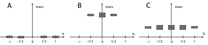
Figure 1: ${\mathcal{N}}=1$ supermultiplets

6 Supercurrents and “central charge”

$U(1)_{R}$ transformation is given by

$$R:~{}\Phi(x,\theta,\bar{\theta})\to e^{i\alpha}\Phi(x,e^{-i\frac{\alpha}{2}}\theta,\bar{\theta}),~{}~{}~{}{\mathcal{W}}_{\alpha}(x,\theta,\bar{\theta})\to{\mathcal{W}}_{\alpha}(x,e^{-i\frac{\alpha}{2}}\theta,\bar{\theta}).$$ (91)

If ${\mathcal{F}}$ transforms as weight two, $R:{\mathcal{F}}\to e^{2i\alpha}{\mathcal{F}}$, then our action is invariant under $R$ and the associated $U(1)_{R}$ current $J^{m}$ is

$${\theta\sigma_{m}\bar{\theta}~{}J^{m}\equiv\theta J\bar{\theta}=(\tau_{2})_{ab}\left(\bar{\theta}\boldsymbol{\bar{\lambda}}^{Ia}~{}\theta\boldsymbol{\lambda}_{I}{}^{b}+iA^{*a}\theta\stackrel{{\scriptstyle\leftrightarrow}}{{{\mathcal{D}}}}_{m}\sigma^{m}\bar{\theta}A^{b}\right)\equiv(\tau_{2})_{ab}\left(\bar{\theta}j^{ab}\theta\right)~{}.}~{}~{}~{}$$ (92)

Acting a supersymmetry transformation on this we obtain ${\mathcal{N}}=2$ supercurrents [21][22]

$${\boldsymbol{\eta}_{J}\boldsymbol{S}^{(J)m}+\boldsymbol{\bar{\eta}}_{J}\boldsymbol{\bar{S}}^{(J)m}=-\frac{1}{2}(\tau_{2})_{ab}~{}{\rm tr}(\bar{\sigma}^{m}\,\boldsymbol{\delta}j^{ab})~{}}$$ (93)

where ${\rm tr}$ is for spinor indices.

Though the $R$-current is not conserved for general ${\mathcal{F}}$, we can construct a conserved ${\mathcal{N}}=2$ supercurrent as a broken ${\mathcal{N}}=2$ supermultiplet of currents. We write ${\mathcal{F}}=\sum_{n}h_{n}C^{(n)}(A^{a})$ where $C^{(n)}(A^{a})$ are $n$-th order $U(N)$ invariant polynomials in $A^{a}$ and $h_{n}$ are their coefficients. First, we assign weight $(2-n)$ to $h_{n}$. Then the weight of ${\mathcal{F}}$ can be regarded as two. The local $U(1)_{R}$ variation of ${\mathcal{L}}$ implies

$${\partial_{m}\left(-\frac{1}{2}{\rm tr}\bar{\sigma}^{m}J\right)=i\left(\sum_{n}(n-2)\frac{\partial}{\partial h_{n}}\right)\mathcal{L}\equiv\Delta_{h}\mathcal{L}~{}.}$$ (94)

Acting the supersymmetry transformation on it, and noting that $\boldsymbol{\delta}{\mathcal{L}}=\partial_{m}X^{m}$ with some $X^{m}$ and that $\Delta_{h}\partial_{m}X^{m}=\partial_{m}\Delta_{h}X^{m}$, we obtain a general construction of the conserved $\mathcal{N}=2$ supercurrents of our model;

$${\boldsymbol{\eta}_{J}\boldsymbol{\mathcal{S}}^{(J)m}+\bar{\boldsymbol{\eta}}^{J}\bar{\boldsymbol{\mathcal{S}}}_{(J)}^{\ m}\equiv-{\frac{1}{2}}{\rm tr}(\bar{\sigma}^{m}\boldsymbol{\delta}J)-\Delta_{h}X^{m}.}$$ (95)

The term $\Delta_{h}X^{m}$ is not universal but depends on the concrete form of ${\mathcal{F}}$. It should be difficult to find the universal coupling to supergravity.

Further action of the supersymmetry transformation generates

$${\theta\boldsymbol{\delta\delta}J\bar{\theta}=8m\xi~{}\bar{\theta}\boldsymbol{\bar{\eta}}\,\boldsymbol{\tau_{1}}\,\boldsymbol{\eta}\theta~{}+~{}\cdots,}$$ (96)

from which we can read off the constant matrix $C_{I}{}^{J}$ in (1) as $C_{I}{}^{J}=+4m\xi(\boldsymbol{\tau}_{1})_{I}{}^{J}$.

7 ${\mathcal{N}}=2$ $U(N)$ gauge model coupled with ${\mathcal{N}}=2$ hypermultiplets

In this section we provide a manifestly ${\mathcal{N}}=2$ supersymmetric formulation of the ${\mathcal{N}}=2$ $U(N)$ gauge model coupled with ${\mathcal{N}}=2$ hypermultiplets[10]. For this we work in harmonic superspace[11] ${\mathbb{R}}^{4|8}\times S^{2}$ parametrized by

$$(x^{m}_{A},\theta^{\pm},\bar{\theta}^{\pm},u_{I}^{\pm})=(x^{m}-2i\theta^{I}\sigma^{m}\bar{\theta}^{J}u_{(I}^{+}u_{J)}^{-},\theta^{I}u_{I}^{\pm},\bar{\theta}^{I}u_{I}^{\pm},u_{I}^{\pm})~{}$$ (97)

in the analytic basis. $u_{I}^{\pm}$ are harmonic variables parametrizing S${}^{2}=SU(2)/U(1)$

$$(u_{I}^{+},u_{I}^{-})\in SU(2)~{},~{}~{}u^{+I}u_{I}^{-}=1~{},~{}~{}\overline{u^{+I}}=u_{I}^{-}~{}.$$ (98)

We introduce an ${\mathcal{N}}=2$ vector multiplet $V^{++}(x^{m},\theta^{+},\bar{\theta}^{+})=V^{++a}t_{a}$ transforming as adjoint under $U(N)$. $V^{++}$ is composed of a complex scalar $A$, a vector $v_{m}$, an $SU(2)$ doublet Weyl spinor $\lambda^{i}_{\alpha}$ and an auxiliary field $D^{IJ}$. $D^{I}{}_{J}=\varepsilon_{JK}D^{IK}=iD^{A}(\tau_{A})^{I}{}_{J}$ is an $SU(2)$ matrix and $D^{A}$ is a real three-vector $\overline{D^{A}}=D^{A}$. By using the field strength $W$ of $V^{++}$ the action for $V^{++}$ is constructed as

$$S_{V} = -\frac{i}{4}\int d^{4}x\left[(D)^{4}{\mathcal{F}}(W)-(\bar{D})^{4}\bar{\mathcal{F}}(\bar{W})\right]~{},$$ (99)

where $(D)^{4}=\frac{1}{16}(D^{+})^{2}(D^{-})^{2}$ and $D^{\pm}$ are the spinor harmonic derivatives[11]. $A$’s parametrize the special Kähler geometry with the Kähler metric $g_{ab}={\rm Im}\,({\mathcal{F}}_{ab}|)$ where ${\mathcal{F}}_{ab\cdots}|$ means ${\mathcal{F}}_{ab\cdots}$ evaluated at $\theta^{\pm}=\bar{\theta}^{\pm}=0$. The metric admits $U(N)$ isometry generated by Killing vectors with the Killing potential ${\cal P}^{a}=-if^{a}_{bc}\bar{A}^{b}A^{c}$.

The ${\mathcal{N}}=2$ hypermultiplet $q^{+}$ is composed of an $SU(2)$ doublet complex scalar $f^{I}$, a pair of $SU(2)$ singlet spinors and infinitely many auxiliary fields. We introduce two sets of ${\mathcal{N}}=2$ hypermultiplets, $N_{f}$ hypermultiplets $q^{+u}$ ($u=1,\cdots,N$) and $N_{a}$ hypermultiplets $q^{+a}$ ($a=0,1,\cdots,N^{2}-1$) which transform as fundamental representation and adjoint representation under $U(N)$, respectively. We suppress flavor indices below. The $U(N)$ gauged action is given by ($\omega$-hypermultiplets are also included in ref.FIS4)

$$S_{q}^{\rm gauged} = -\int dud\zeta^{(-4)}\left[\tilde{q}^{+}_{u}{\mathcal{D}}^{++}q^{+u}+\tilde{q}^{+}_{a}{\mathcal{D}}^{++}q^{+a}\right]~{}$$ (100)

where the tilde denotes the analyticity preserving conjugation[11]. The covariant derivative is defined as ${\mathcal{D}}^{++}q^{+\mu}=D^{++}q^{+\mu}+iV^{++a}(T_{a})^{\mu}{}_{\nu}q^{+\nu}$ where $D^{++}$ is the harmonic derivative[11] and

$$(T_{a})^{\mu}{}_{\nu}=\left\{\!\!\!\begin{array}[]{ll}(t_{a})^{u}{}_{v}&\mbox{for fundamental}~{}q^{+}\\ {\rm ad}(t_{a})^{b}{}_{c}=if^{b}_{ac}&\mbox{for adjoint}~{}q^{+}\\ \end{array}\right..$$ (103)

The $U(N)$ isometry gauged above is generated by Killing vectors with Killing potentials

$$\left\{\begin{array}[]{l}\hat{\mathcal{Q}}^{IJ}_{a}={\mathcal{Q}}^{IJ}_{a}|_{T_{a}=t_{a}}\\ \check{\mathcal{Q}}^{IJ}_{a}={\mathcal{Q}}^{IJ}_{a}|_{T_{a}={\rm ad}(t_{a})}\\ \end{array}\right.~{}~{}\mbox{where}~{}~{}~{}{\mathcal{Q}}^{IJ}_{a}=i\bar{f}^{(I}_{\mu}(T_{a})^{\mu}{}_{\nu}f^{J)\nu}~{}.$$ (106)

Next we introduce the electric and magnetic FI terms. The electric FI term is given by

$$S_{e} = \int dud\zeta^{(-4)}{\rm tr}(\Xi^{++}V^{++})+c.c.=\int d^{4}x\xi^{IJ}D^{0}_{IJ}+c.c.$$ (107)

where $\Xi^{++}=\xi^{IJ}u_{I}^{+}u_{J}^{+}$ is the electric FI parameter. The effect of this term is to shift the dual auxiliary field $D_{D}^{aIJ}$ in $W_{D}^{a}\equiv{\mathcal{F}}_{a}$ by an imaginary constant, $D_{D}^{aIJ}\to D_{D}^{aIJ}+8i\xi_{D}^{IJ}\delta_{0}^{a}$. We introduce the magnetic FI term so as to shift the auxiliary field $D^{aIJ}$ in $W^{a}$ by an imaginary constant, $D^{aIJ}\to\boldsymbol{D}^{aIJ}=D^{aIJ}+4i\xi^{IJ}\delta_{0}^{a}$. By this, the ${\mathcal{N}}=2$ supersymmetry transformation law $\delta_{\eta}\lambda^{aI}=(D^{a})^{I}{}_{J}\eta^{J}+\cdots$ changes to $\delta_{\eta}\lambda^{aI}=(\boldsymbol{D}^{a})^{I}{}_{J}\eta^{J}+\cdots$, under which the total action

$$S=S_{V}+S^{\rm gauged}_{q}+S_{e}+S_{m}$$ (108)

is invariant. It is straightforward to see that the magnetic FI term of the form

$$S_{m} = \int d^{4}x\left[(D)^{4}\xi_{D}^{IJ}\theta_{I}\theta_{J}\left({\mathcal{F}}_{0}+2i{\mathcal{F}}_{00}\xi_{D}^{KL}\theta_{K}\theta_{L}\right)+2i\hat{\mathcal{Q}}^{IJ}_{0}\xi_{DIJ}\right]+c.c.$$ (109)

causes the imaginary constant shift of the auxiliary field

$$S_{V}+S^{\rm gauged}_{q}+S_{m}=\left.\left(S_{V}+S^{\rm gauged}_{q}\right)\right|_{D\to\boldsymbol{D}}~{}$$ (110)

where $|_{D\to\boldsymbol{D}}$ means the replacement $D^{aIJ}\to\boldsymbol{D}^{aIJ}$ ($D^{aIJ}\to\bar{\boldsymbol{D}}^{aIJ}$). We find that in the presence of hypermultiplets in the fundamental representation of the gauge group $U(N)$, the magnetic FI term develops an additional term which overcomes the difficulty in coupling fundamental hypermultiplets with the APT model. The adjoint scalars do not appear in (109) because ${\rm ad}(t_{0})=0$.

It is straightforward to eliminate infinitely many auxiliary fields in $q^{+}$ and the auxiliary field $D$ in $V^{++}$ and obtain the scalar potential

$${\cal V} = \frac{1}{4}g_{ab}\boldsymbol{D}^{aIJ}|\bar{\boldsymbol{D}}^{b}_{IJ}|+g_{ab}{\cal P}^{a}{\cal P}^{b}+2i(\xi^{IJ}+\bar{\xi}^{IJ})(\xi_{DIJ}-\bar{\xi}_{DIJ})$$ (111)

$$+\overline{f^{I}}_{u}(\bar{A}A+A\bar{A})^{u}{}_{v}f^{Iv}+\overline{f^{I}}_{a}(\bar{A}A+A\bar{A})^{a}{}_{b}f^{Ib}$$

where

$$\boldsymbol{D}^{aIJ}|=-2g^{ab}\left[(\xi^{IJ}+\bar{\xi}^{IJ})\delta_{b}^{0}+(\xi_{D}^{IJ}+\bar{\xi}_{D}^{IJ})\bar{\mathcal{F}}_{0b}|+\hat{\mathcal{Q}}^{IJ}_{b}+\check{\mathcal{Q}}^{IJ}_{b}\right]~{}.$$

The vacua are determined by ${\cal V}$ and exhibit various phases. On the Coulomb phase $\langle\!\langle A^{\underline{i}}\rangle\!\rangle\neq 0$, $\langle\!\langle A^{r}\rangle\!\rangle=\langle\!\langle f^{I}_{u}\rangle\!\rangle=\langle\!\langle f^{I}_{r}\rangle\!\rangle=0$ and thus $\langle\!\langle\hat{\mathcal{Q}}_{b}^{IJ}\rangle\!\rangle=\langle\!\langle\check{\mathcal{Q}}_{b}^{IJ}\rangle\!\rangle=0$. In this way we have arrived at the vacuum condition for ${\mathcal{N}}=2$ $U(N)$ gauge model without hypermultiplets, $\langle\!\langle\partial_{A^{a}}{\cal V}\rangle\!\rangle=\frac{i}{4}\langle\!\langle{\mathcal{F}}_{abc}|\boldsymbol{D}^{bA}\boldsymbol{D}^{cA}\rangle\!\rangle=0$. Let us examine the case with ${\mathcal{F}}=\sum_{n}\frac{c_{n}}{n!}{\rm tr}W^{n}$ for concreteness. Then it further reduces to

$$\sum_{A}\langle\!\langle\boldsymbol{D}^{\underline{i}A}\boldsymbol{D}^{\underline{i}A}\rangle\!\rangle=0~{},~{}~{}~{}\underline{i}=\underline{1},\cdots,\underline{N}~{}.$$ (112)

It is easy to show that by fixing $SU(2)$ appropriately $\langle\!\langle{\mathcal{F}}_{\underline{i}\underline{i}}\rangle\!\rangle=-2(\frac{e}{m}\pm i\frac{\xi}{m})$ in (56) can be reproduced. On the vacua the supersymmetry transformations of fermions are found to be trivial except for

$$\langle\!\langle\delta\lambda^{\underline{i}I}\rangle\!\rangle=i\langle\!\langle\boldsymbol{D}^{\underline{i}A}\rangle\!\rangle(\tau_{A})^{I}{}_{J}\eta^{J}~{}.$$ (113)

On the other hand the mass term of $\lambda^{\underline{i}I}$ is

$$-\frac{i}{4}\langle\!\langle{\mathcal{F}}_{\underline{i}\underline{i}\underline{i}}\boldsymbol{D}^{\underline{i}A}\rangle\!\rangle\lambda^{\underline{i}I}(\tau_{2}\tau_{A})_{IJ}\lambda^{\underline{i}J}~{}.$$ (114)

Because (112) implies that $\det\boldsymbol{D}^{\underline{i}}{}^{I}{}_{J}=0$, a half of the fermions $\lambda^{\underline{i}I}$, $I=1,2$, say $U^{1}{}_{J}\lambda^{\underline{i}J}$ with a constant matrix $U^{I}{}_{J}$, is massless but has a nontrivial supersymmetry transformation. In the ordinary basis spanned by matrices $t_{a}$, this means that $U^{1}{}_{J}\lambda^{0J}$ is the NG fermion for partial supersymmetry breaking.

References

- [1] J. T. Lopuszanski, “The Spontaneously Broken Supersymmetry In Quantum Field Theory,” Rept. Math. Phys. 13 (1978) 37.
- [2] I. Antoniadis, H. Partouche and T. R. Taylor, “Spontaneous Breaking of Global Supersymmetry,” Phys. Lett. B 372 (1996) 83 [arXiv:hep-th/9512006].
- [3] S. Ferrara, L. Girardello and M. Porrati, “Spontaneous Breaking of N=2 to N=1 in Rigid and Local Supersymmetric Theories,” Phys. Lett. B 376 (1996) 275 [arXiv:hep-th/9512180].
- [4] H. Partouche and B. Pioline, “Partial spontaneous breaking of global supersymmetry,” Nucl. Phys. Proc. Suppl. 56B (1997) 322 [arXiv:hep-th/9702115].
- [5] E. A. Ivanov and B. M. Zupnik, “Modified N = 2 supersymmetry and Fayet-Iliopoulos terms,” Phys. Atom. Nucl. 62 (1999) 1043 [Yad. Fiz. 62 (1999) 1110] [arXiv:hep-th/9710236].
- [6] R. Grimm, M. Sohnius and J. Wess, “Extended Supersymmetry And Gauge Theories,” Nucl. Phys. B 133 (1978) 275; M. F. Sohnius, “Bianchi Identities For Supersymmetric Gauge Theories,” Nucl. Phys. B 136 (1978) 461; M. de Roo, J. W. van Holten, B. de Wit and A. Van Proeyen, “Chiral Superfields In N=2 Supergravity,” Nucl. Phys. B 173 (1980) 175.
- [7] K. Fujiwara, H. Itoyama and M. Sakaguchi, “Supersymmetric gauge model and partial breaking of supersymmetry,” Prog. Theor. Phys. 133 (2005) 429 [arXiv:hep-th/0409060].
- [8] K. Fujiwara, H. Itoyama and M. Sakaguchi, “ gauge model and partial breaking of supersymmetry,” in the proceedings of SUSY2004 [arXiv:hep-th/0410132].
- [9] K. Fujiwara, H. Itoyama and M. Sakaguchi, “Partial breaking of supersymmetry and of gauge symmetry in the gauge model,” Nucl. Phys. B 723 (2005) 33 [arXiv:hep-th/0503113].
- [10] K. Fujiwara, H. Itoyama and M. Sakaguchi, “Partial supersymmetry breaking and U(Nc) gauge model with hypermultiplets in harmonic superspace,” Nucl. Phys. B in press [arXiv:hep-th/0510255].
- [11] A. S. Galperin, E. A. Ivanov, V. I. Ogievetsky and E. S. Sokatchev, “Harmonic superspace,” Cambridge University Press, 2001.
- [12] N. Seiberg and E. Witten, “Electric - magnetic duality, monopole condensation, and confinement in N = 2 supersymmetric Yang-Mills theory,” Nucl. Phys. B 426 (1994) 19 [Erratum-ibid. B 430 (1994) 485] [arXiv:hep-th/9407087].
- [13] T. R. Taylor and C. Vafa, “RR flux on Calabi-Yau and partial supersymmetry breaking,” Phys. Lett. B 474 (2000) 130 [arXiv:hep-th/9912152]; P. Mayr, “On supersymmetry breaking in string theory and its realization in brane worlds,” Nucl. Phys. B 593 (2001) 99 [arXiv:hep-th/0003198]; C. Vafa, “Superstrings and topological strings at large N,” J. Math. Phys. 42 (2001) 2798 [arXiv:hep-th/0008142]; F. Cachazo, K. A. Intriligator and C. Vafa, “A large N duality via a geometric transition,” Nucl. Phys. B 603 (2001) 3 [arXiv:hep-th/0103067]; F. Cachazo, S. Katz and C. Vafa, “Geometric transitions and N = 1 quiver theories,” arXiv:hep-th/0108120; F. Cachazo, B. Fiol, K. A. Intriligator, S. Katz and C. Vafa, “A geometric unification of dualities,” Nucl. Phys. B 628 (2002) 3 [arXiv:hep-th/0110028]; J. Louis and A. Micu, “Type II theories compactified on Calabi-Yau threefolds in the presence of background fluxes,” Nucl. Phys. B 635 (2002) 395 [arXiv:hep-th/0202168]; F. Cachazo and C. Vafa, “N = 1 and N = 2 geometry from fluxes,” arXiv:hep-th/0206017.
- [14] R. Dijkgraaf and C. Vafa, “Matrix models, topological strings, and supersymmetric gauge theories,” Nucl. Phys. B 644 (2002) 3 [arXiv:hep-th/0206255]; R. Dijkgraaf and C. Vafa, “On geometry and matrix models,” Nucl. Phys. B 644 (2002) 21 [arXiv:hep-th/0207106]; R. Dijkgraaf and C. Vafa, “A perturbative window into non-perturbative physics,” arXiv:hep-th/0208048; H. Itoyama and A. Morozov, “The Dijkgraaf-Vafa prepotential in the context of general Seiberg-Witten theory,” Nucl. Phys. B 657 (2003) 53 [arXiv:hep-th/0211245].
- [15] F. Cachazo, M. R. Douglas, N. Seiberg and E. Witten, “Chiral rings and anomalies in supersymmetric gauge theory,” JHEP 0212, 071 (2002) [arXiv:hep-th/0211170].
- [16] P. Kaste and H. Partouche, “On the equivalence of N = 1 brane worlds and geometric singularities with flux,” JHEP 0411 (2004) 033 [arXiv:hep-th/0409303].
- [17] A. Morozov, “Challenges of matrix models,” arXiv:hep-th/0502010.
- [18] J. Bagger and E. Witten, “The Gauge Invariant Supersymmetric Nonlinear Sigma Model,” Phys. Lett. B 118, 103 (1982).
- [19] C. M. Hull, A. Karlhede, U. Lindstrom and M. Rocek, “Nonlinear Sigma Models And Their Gauging In And Out Of Superspace,” Nucl. Phys. B 266, 1 (1986).
- [20] P. Fayet and J. Iliopoulos, “Spontaneously Broken Supergauge Symmetries And Goldstone Spinors,” Phys. Lett. B 51 (1974) 461; P. Fayet, “Fermi-Bose Hypersymmetry,” Nucl. Phys. B 113 (1976) 135.
- [21] S. Ferrara and B. Zumino, “Transformation Properties Of The Supercurrent,” Nucl. Phys. B 87, 207 (1975).
- [22] H. Itoyama, M. Koike and H. Takashino, “N = 2 supermultiplet of currents and anomalous transformations in supersymmetric gauge theory,” Mod. Phys. Lett. A 13, 1063 (1998) [arXiv:hep-th/9610228].