Probabilities in the landscape

Abstract

I review recent progress in defining probability distributions in the inflationary multiverse.

I Introduction

It has long been a dream of particle physicists to derive the values of all constants of Nature from a fundamental theory. With the development of string theory in the last few decades, it seemed for a while that we were getting closer to that goal. String theory is our best candidate for the fundamental theory, and there has been great enthusiasm and hope that it will yield a unique set of constants. This hope, however, appears to have been dashed. It now appears that string theory has a multitude of solutions describing vacua with different values of the low-energy constants. The number of vacua in this vast “landscape” of possibilities can be as large as $10^{500}$ BP ; Susskind ; Douglas .

In the cosmological context, high-energy vacua will drive exponential inflationary expansion of the universe. Transitions between different vacua will occur through quantum tunneling, with bubbles of different vacua nucleating and expanding in the never-ending process of eternal inflation. As a result, the entire landscape of vacua will be explored.

If indeed this kind of picture describes our universe, then we will never be able to calculate all constants of Nature from first principles. At best we may only be able to make statistical predictions. The key problem is then to calculate the probability distribution for the constants. It is often referred to as the measure problem.

The probability $P_{j}$ of observing vacuum $j$ can be expressed as a product AV95

$$P_{j}=P_{j}^{(V)}n_{j}^{(obs)},$$ (1)

where $P_{j}^{(V)}$ is the fraction of volume occupied by vacuum of type $j$ and $n_{j}^{(obs)}$ is the number of observers per unit volume. The distribution (1) then gives the probability for a randomly picked observer to be in a vacuum of type $j$.

The density of observers $n_{j}^{(obs)}$ cannot at present be calculated, but in many interesting cases it seems reasonable to approximate it as being proportional to the density of suitable stars, which is in turn proportional to the fraction of matter clustered in giant galaxies AV96 ; Weinberg96 ; MSW .

The volume factor $P_{j}^{(V)}$ presents a problem of a very different kind: the result depends very sensitively on the choice of a spacelike hypersurface (a constant-time surface) on which the distribution is to be evaluated. This problem was uncovered by Andrei Linde and his collaborators when they first attempted to calculate volume distributions LLM ; LM ; GBL . It eluded resolution for more than a decade, but recently there have been some promising developments, and I believe we are getting close to completely solving the problem. The purpose of this paper is to review the new proposals for $P_{j}^{(V)}$.

II Problem with global-time measure

The spacetime structure of an eternally inflating universe is schematically illustrated in Fig.1. The bubbles expand rapidly approaching the speed of light, so their worldsheets are well approximated by light cones. If the vacuum inside a bubble has positive energy density, it becomes a site of further bubble nucleation; we call such vacua “recyclable”. Negative-energy vacua, on the other hand, quickly develop curvature singularities; we shall call them “terminal vacua”.

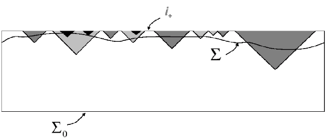
Figure 1: A schematic conformal diagram for a comoving region in an eternally inflating universe. Bubbles of different vacua are represented by different shades of gray. The upper boundary of the diagram $i_{+}$ is the future timelike infinity. A surface of constant global time $\Sigma$ cuts through the entire region and intersects many bubbles.

The diagram represents a comoving region, which is initially comparable to the horizon. The initial moment is a spacelike hypersurface $\Sigma_{0}$, represented by the lower horizontal boundary of the diagram, while the upper boundary represents future infinity, when the region and all the bubbles become infinitely large. How can we find the fraction of volume occupied by different vacua? A natural thing to do is to consider a spacelike hypersurface $\Sigma$, which cuts through the entire region, as shown in the figure. If $t$ is a globally defined time coordinate, then all surfaces $t={\rm const}$ will have this property. One can use, for example, the proper time along the “comoving” geodesics orthogonal to the surface $\Sigma_{0}$. Alternatively, one could use the so-called scale factor time, defined as a logarithm of the expansion factor along the comoving geodesics, or any other suitable time coordinate. Once the time coordinate is specified, one can find the fraction of volume occupied by different vacua on the surface $t={\rm const}$ and then take the limit $t\to\infty$.

Unfortunately, as I have already mentioned, the result of this calculation is sensitively dependent on one’s choice of the time coordinate LLM . The reason is that the volume of an eternally inflating universe is growing exponentially with time. The volumes of regions filled with all possible vacua are growing exponentially as well. At any time, a substantial part of the total volume is in new bubbles which have just nucleated. Which of these bubbles are cut by the surface depends on how the surface is drawn; hence the gauge-dependence of the result. Since time is an arbitrary label in General Relativity, none of the possible choices of the global time coordinate appears to be preferred. For more discussion of this gauge-dependence problem, see Guth ; Tegmark ; Winitzki1 .

III A pocket-based measure

It is now becoming increasingly clear that the solution to the problem lies in the direction of using the local definition of time within individual bubbles, or, as Alan Guth called them, “pocket universes”. I will first discuss how this works in the simplest case, when there is a single type of bubble; the general situation will be considered in the next section.

Suppose we have an eternally inflating universe filled with a metastable false vacuum $F$, which decays to the true vacuum $T$ through bubble nucleation. The vacuum energy is thermalized within the bubbles, and in due course observers evolve there and measure the constants of Nature. Suppose further that there is a scalar field $X$, which affects the values of some constants and has a very slowly varying potential $U(X)$. The values of $X$ are randomized by quantum fluctuations during inflation, so $X$ is slowly varying in space within each bubble. We shall assume that the slope of $U(X)$ is so small that time variation of $X$ is negligible during the epoch when the observers are present. Our goal is to find the distribution

$$P^{(V)}(X)dX,$$ (2)

which gives the volume fraction occupied by regions where the field is in the interval between $X$ and $X+dX$.

A measure based on a global time coordinate runs into the same problem as in the case of a discrete distribution $P_{j}^{(V)}$: the result for $P^{(V)}(X)$ is gauge-dependent. There is, however, a simple way around this difficulty GTV ; AV98 ; VVW . It is well known CdL that bubble interiors appear to their inhabitants as self-contained infinite universes of negative curvature. A natural definition of the time coordinate in such a universe is to identify it with one of the physical variables, e.g., the energy density. Each pocket universe will then have its own set of infinite constant-time surfaces (see Fig.2).

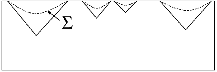
Figure 2: A comoving region with a single type of bubble. Bubbles differ by details of the scalar field distribution, but are statistically identical. Each pocket is internally an infinite open universe. Constant-time surfaces within pockets, shown by dashed lines, are infinite spacelike surfaces.

The proposal of GTV ; AV98 ; VVW is to calculate the distribution (2) within a single pocket universe. It does not matter which one, since all pocket universes are statistically equivalent: they all have the same volume distribution of $X$.

Once a pocket universe is selected, we choose some constant-time surface within it as our reference surface $\Sigma$. The next step is to find the volume distribution of $X$ on $\Sigma$. Some care is needed here, since $\Sigma$ is an infinite hypersurface. If one calculates the distribution in a region of finite size and then takes the limit of size going to infinity, the result may depend on the limiting procedure. To avoid this danger, one has to make sure that the shape of the region is not correlated with the distribution of $X$. The simplest choice is to use a “spherical” region, defined as a set of points with a geodesic distance $r<R$ from a given center, with the limit $R\to\infty$ taken afterwards AV98 ; VVW .

Since we assume that $X$ does not change in time, its value remains constant along the comoving geodesics, and thus the distribution (2) is time-independent if we think of it as a comoving-volume distribution. The density of observers $n^{(obs)}(X)$ should then also be understood as the number of observers per unit comoving volume. If we include all present, past and future observers, then $n^{(obs)}(X)$ is also time-independent. Moreover, the full distribution

$$dP(X)\propto P^{(V)}(X)n^{(obs)}(X)$$ (3)

does not depend on the choice of the reference hypersurface $\Sigma$, as long as $P^{(V)}(X)$ and $n^{(obs)}(X)$ are evaluated on the same hypersurface.

Some analytic and numerical techniques for calculating $P^{(V)}(X)$ have been suggested in GTV ; AV98 ; VVW . These techniques are not yet fully developed, and there are some interesting issues that still need to be addressed (e.g., the “ergodic conjecture” in Ref. GSPVW ). But as a matter of principle, the problem appears to have been solved in the case of identical pockets.

IV Counting pockets

If there are many different types of pockets, then it is clearly not sufficient to consider a single bubble. We have to learn how to compare the numbers of observers in different bubbles. Since the bubbles are disconnected from one another, we have to define a comoving length scale $R_{j}$ on which observers are to be counted in bubbles of type $j$. In addition, some bubbles may be more abundant than others, and we have to introduce a frequency factor $p_{j}$ characterizing the relative abundance of different bubbles. The full expression for the volume distribution is then given by markers

$$P_{j}^{(V)}\propto p_{j}R_{j}^{3}.$$ (4)

Here I assume for simplicity that there are no continuous fields $X$ that can vary within bubbles. The discussion can be easily extended to include such variables (see Sec.IV.D). The question now is: How do we define $p_{j}$ and $R_{j}$? We shall consider them in turn.

IV.1 Bubble abundance $p_{j}$

The definition of $p_{j}$ is a tricky business, because the total number of bubbles is infinite, even in a region of a finite comoving size. We thus need to introduce some sort of a cutoff. Here I shall review the procedure recently proposed in GSPVW , which has some attractive properties.

The proposal is very simple: count only bubbles greater than a certain comoving size $\epsilon$, and then take the limit $\epsilon\to 0$. To define the comoving size, one has to specify a congruence of “comoving” geodesics emanating from some initial spacelike hypersurface $\Sigma_{0}$. As they extend to the future, the geodesics will generally cross a number of bubbles before ending up in one of the terminal bubbles, where inflation comes to an end. There will also be a (measure zero) set of geodesics which never hit terminal bubbles. The starting points of these geodesics on $\Sigma_{0}$ provide a mapping of the eternally inflating fractal Aryal ; Winitzki ; Winitzki2 , consisting of points on $i_{+}$ where inflation never ends. In the same manner, each bubble encountered by the geodesics will also be mapped on $\Sigma_{0}$, and we can define the “size” of a bubble as the volume of its image on $\Sigma_{0}$. (The volume of a bubble is calculated including all the daughter bubbles that nucleate within it.)

In an inflating spacetime, geodesics are rapidly diverging, so bubbles formed at later times have a smaller comoving size. (The comoving size of a bubble is set by the horizon at the time of bubble nucleation.) The bubble counting can be done in an arbitrarily small neighborhood $\delta$ of any point belonging to the “eternal fractal” image on $\Sigma_{0}$. Every such neighborhood will contain an infinite number of bubbles of all kinds and will be dominated by bubbles formed at very late times and having very small comoving sizes. The resulting values of $p_{j}$, obtained in the limit of bubble size $\epsilon\to 0$, will be the same in all neighborhoods, because of the universal asymptotic behavior of eternal inflation.

It is clear that the same result will also hold in any finite-size region on $\Sigma_{0}$ (provided that it contains at least one “eternal point”), and for any choice of the initial hypersurface $\Sigma_{0}$. Moreover, although we use the metric on $\Sigma_{0}$ to compare the bubble sizes, the results are unaffected by smooth conformal transformations of the metric. Any such transformation will locally be seen as a linear transformation, which amounts to a constant rescaling of bubble sizes. In a sufficiently small neighborhood on $\Sigma_{0}$, all bubble sizes are rescaled in the same way, so the bubble counting should not be affected.

The results obtained using this method are also independent of the initial conditions at the onset of eternal inflation. This is an attractive property, since the initial conditions are quickly forgotten in an eternally inflating universe.

The calculation of bubble abundances, defined in this way, can be reduced to an eigenvalue problem for a matrix constructed out of the transition rates between different vacua GSPVW . This prescription has been tried in some simple models and appears to give reasonable results GSPVW ; SPV . For example, if there is a single false vacuum, which can decay into a number of vacua with nucleation rates $\Gamma_{j}$ , one finds

$$p_{j}\propto\Gamma_{j},$$ (5)

as intuitively expected.

IV.2 An equivalent proposal

An alternative prescription for $p_{j}$ has been suggested by Easther, Lim and Martin ELM . They randomly select a large number $N$ of worldlines out of a congruence of comoving geodesics and define $p_{j}$ as being proportional to the number of bubbles of type $j$ intersected by at least one of these worldlines in the limit of $N\to\infty$.

As the number of worldlines is increased, the average comoving distance $\epsilon$ between them gets smaller, so most bubbles of comoving size larger than $\epsilon$ are counted. In the limit of $N\to\infty$, we have $\epsilon\to 0$, and it is not difficult to see that this prescription is equivalent to the one described in the preceding subsection. (For a rigorous proof, see Note added in GSPVW .)

IV.3 Reference length $R_{j}$

Our next task is to define the comoving reference scale $R_{j}$. The first thing that comes to mind is to set $R_{j}$ to be the same for all bubbles. However, this is not enough. The expansion rate is different in different bubbles, so the physical length scales corresponding to $R_{j}$ will not stay equal, even if they were equal at some moment. We could specify the times $t_{j}$ at which $R_{j}$ are set to be equal, but any such choice would be subject to the criticism of being arbitrary.

A possible way around this difficulty was proposed in GSPVW . At early times after nucleation, the dynamics of open FRW universes inside bubbles is dominated by curvature, with the scale factor given by

$$a_{j}(t)\approx t$$ (6)

for all types of bubbles. For example, for a quasi-de Sitter bubble interior,

$$a_{j}(t)\approx H_{j}^{-1}\sinh(H_{j}t),$$ (7)

where $H_{j}=(8\pi G\rho_{j}/3)^{1/2}$ is the expansion rate corresponding to the local vacuum energy density $\rho_{j}$. The specific form of the scale factor at late times is not important for our argument. The point is that for $t\ll H_{j}^{-1}$ all bubbles are nearly identical, with the scale factor (6). (This is basically a consequence of the universal spacetime structure in the vicinity of the light cone $t=0$.)

The proposal of GSPVW is that the reference scales should be chosen so that $R_{j}$ are the same at some small $t=\tau$. The choice of $\tau$ is unimportant, as long as $\tau\ll H_{j}^{-1}$ for all $j$. Then, up to a constant, the physical length corresponding to $R_{j}$ is

$$R_{j}(t)=a_{j}(t).$$ (8)

For times $t\gg H_{j}^{-1}$, this can be expressed as

$$R_{j}(t)\approx H_{j}^{-1}Z_{j}(t),$$ (9)

where $Z_{j}$ is the expansion factor since the onset of the inflationary expansion inside the bubble ($t\sim H_{j}^{-1}$).

Alternatively, $R_{j}$ in (9) can be identified as the curvature scale. It is the characteristic large-scale curvature radius of the bubble universe. This definition makes no reference to early times close to the bubble nucleation: the curvature radius can be found at any time. It is, in principle, a measurable quantity.

IV.4 Continuous variables

The prescription (4) can be straightforwardly generalized to the case when, in addition to bubbles, there are some continuously varying fields $X$:

$$P_{j}^{(V)}(X)\propto p_{j}{\hat{P}}_{j}(X)R_{j}^{3}(X).$$ (10)

Here, ${\hat{P}}_{j}(X)$ is the normalized distribution for $X$ in a bubble of type $j$ at $t=\tau\ll H_{j}^{-1}$,

$$\int{\hat{P}}_{j}(X)dX=1.$$ (11)

This distribution can be calculated analytically or numerically, using the methods of Refs. VVW ; GSPVW .

V Discussion

The above definition of the measure is just a proposal. We have not derived it from first principles. In fact, there is no guarantee that there is some unique measure that can be used for making predictions in the multiverse. How, then, can we ever know that we made the right choice out of all possible options?

What I find encouraging is that even a single definition of measure that satisfies some basic requirements proved very difficult to find. In addition to being mathematically consistent, we require that the measure should not depend on any arbitrary choices, such as the choice of gauge or of a spacelike hypersurface, and that it should be independent of the initial conditions at the onset of inflation. It would be interesting to know how much freedom is left by these requirements. In other words, how uniquely do they specify the proposal of Ref. GSPVW ?

The measure can further be tested by working out simple models and checking whether or not the resulting distributions are reasonable. So far, the proposal of GSPVW seems to have passed this test.

A possible alternative, advocated in Tegmark , is to assume that “all infinities are equal” and set

$$p_{j}={\rm const}$$ (12)

for all $j$. This prescription is clearly gauge-invariant and is independent of the initial conditions. The resulting measure, however, appears to be counter-intuitive. Intuitively, one expects that, everything else being equal, the probability assigned to a certain type of bubble should be proportional to the bubble nucleation rate. This is satisfied for the proposal of GSPVW , but if (12) is adopted, the probability would be completely independent of the nucleation rate.

The ultimate test of any proposed measure will be a comparison of its predictions with observations. The first attempts in this direction have already produced some intriguing results Aguirre ; Freivogel ; Hall1 ; QLambda ; Tegmark2 ; Hall2 ; SPV ; Hawking . It seems safe to predict that we will hear more on this subject in the future.

I am grateful to Leonard Susskind for pointing out an error in the original version of this paper and for stimulating correspondence. I am also grateful to Jaume Garriga, Delia Schwartz-Perlov and Serge Winitzki for discussions and useful comments. This work was supported in part by the National Science Foundation.

References

- (1) R. Bousso and J. Polchinski, JHEP 0006, 006 (2000).
- (2) L. Susskind, “The anthropic landscape of string theory,” arXiv:hep-th/0302219.
- (3) M.R. Douglas, JHEP 0305, 046 (2003).
- (4) A. Vilenkin, Phys. Rev. Lett. 74, 846 (1995).
- (5) A. Vilenkin, in Cosmological Constant and the Evolution of the Universe, ed by K. Sato, T. Suginohara and N. Sugiyama (Universal Academy Press, Tokyo, 1996).
- (6) S. Weinberg, in Critical Dialogues in Cosmology, ed. by N. G. Turok (World Scientific, Singapore, 1997).
- (7) H. Martel, P. R. Shapiro and S. Weinberg, Ap.J. 492, 29 (1998).
- (8) A. D. Linde, D. A. Linde, and A. Mezhlumian, Phys. Rev. D 49, 1783 (1994)
- (9) A. D. Linde and A. Mezhlumian, Phys. Rev. D 53, 4267 (1996)
- (10) J. Garcia-Bellido and A. D. Linde, Phys. Rev. D 51, 429 (1995).
- (11) A. H. Guth, Phys. Rept. 333, 555 (2000)
- (12) M. Tegmark, JCAP 0504, 001 (2005)
- (13) S. Winitzki, Phys. Rev. D 71, 123507 (2005).
- (14) J. Garriga, T. Tanaka, and A. Vilenkin, Phys. Rev. D 60, 023501 (1999)
- (15) A. Vilenkin, Phys. Rev. Lett. 81, 5501 (1998)
- (16) V. Vanchurin, A. Vilenkin, and S. Winitzki, Phys. Rev. D 61, 083507 (2000)
- (17) S Coleman and F. DeLuccia, Phys. Rev. D21, 3305 (1980).
- (18) J. Garriga, D. Schwartz-Perlov, A. Vilenkin and S. Winitzki, JCAP 0601, 017 (2006). “Probabilities in the inflationary multiverse”, hep-th/0509184.
- (19) J. Garriga and A. Vilenkin, Phys. Rev. D 64, 023507 (2001)
- (20) M. Aryal and A. Vilenkin, Phys. Lett. B199, 352 (1987).
- (21) S. Winitzki, Phys. Rev. D65, 083506 (2002).
- (22) S. Winitzki, Phys. Rev. D71, 123523 (2005).
- (23) J. Garriga and A. Vilenkin, unpublished.
- (24) D. Schwartz-Perlov and A. Vilenkin, “Probabilities in the Bousso-Polchinski multiverse”, hep-th/0601162.
- (25) R. Easther, E.A. Lim and W.R. Martin, “Counting pockets with worldlines in eternal inflation”, astro-ph/0511233.
- (26) A. Aguirre and M. Tegmark, JCAP 0501, 003 (2005).
- (27) B. Freivogel, M. Kleban, M. Rodrigues Martinez, and L. Susskind, “Observational consequences of a landscape”, hep-th/0505232.
- (28) B. Feldstein, L.J. Hall and T. Watari, Phys. Rev. D72, 123506 (2005).
- (29) J. Garriga and A. Vilenkin, “Anthropic predictions for and the catastrophe”, hep-th/0508005.
- (30) M. Tegmark, A. Aguirre, M. Rees and F. Wilczek, “Dimensionless constants, cosmology and other dark matters”, astro-ph/0511774.
- (31) L.J. Hall, T. Watari and T.T. Yanagida, “Taming the runaway problem of inflationary landscapes”, hep-th/0601028.
- (32) S.W. Hawking and T. Hertog, “Populating the landscape: a top down approach”, hep-th/0602091.