Curved Superspaces and Local Supersymmetry
in Supermatrix Model

Abstract

In a previous paper, we introduced a new interpretation of matrix models, in which any $d$-dimensional curved space can be realized in terms of $d$ matrices, and the diffeomorphism and the local Lorentz symmetries are included in the ordinary unitary symmetry of the matrix model. Furthermore, we showed that the Einstein equation is naturally obtained, if we employ the standard form of the action, $S=-tr\left([A_{a},A_{b}][A^{a},A^{b}]\right)+\cdots$. In this paper, we extend this formalism to include supergravity. We show that the supercovariant derivatives on any $d$-dimensional curved space can be expressed in terms of $d$ supermatrices, and the local supersymmetry can be regarded as a part of the superunitary symmetry. We further show that the Einstein and Rarita-Schwinger equations are compatible with the supermatrix generalization of the standard action.

1 Introduction

Although it is believed that string theory can provide a formalism describing the unification of the fundamental interactions, its present formulation based on perturbation theory is not satisfactory. In order to examine whether it actually describes our four-dimensional world, a non-perturbative, background independent formulation is needed. Matrix models represent a promising approach to the study of the nonperturbative dynamics of string theory. For critical strings, they are basically obtained through dimensional reduction of the ten-dimensional $U(N)$ ${\cal N}=1$ supersymmetric Yang-Mills theory [2, 3].

IIB matrix model [3] is obtained through dimensional reduction to a point, and the action is given by

$$S=-\frac{1}{g^{2}}tr\left(\frac{1}{4}[A_{a},A_{b}][A^{a},A^{b}]+\frac{1}{2}\bar{\psi}\gamma^{a}[A_{a},\psi]\right),$$ (1)

where $\psi$ is a ten-dimensional Majorana-Weyl spinor, and $A_{a}$ and $\psi$ are $N\times N$ Hermitian matrices. The indices $a$ and $b$ are contracted by the flat metric. This action has an $SO(10)$ global Lorentz symmetry and $U(N)$ symmetry. A problem with this model is that it is unclear how curved spaces are described and how the fundamental principle of general relativity is realized in it.

It may seem that the space of dynamical variables would become very small through the dimensional reduction, but this is not the case if $N$ is infinitely large [4]. Indeed, IIB matrix model contains super Yang-Mills theory:

$$\mbox{$10D$ super Yang-Mills}\overset{{\rm dim.red.}}{\longrightarrow}\mbox{IIB matrix model}\overset{N\to\infty}{\supset}\mbox{$10D$ super Yang-Mills}.$$

The matrix-valued variables $A_{a}$ and $\psi_{\alpha}$ act on the Hilbert space $V={\mathbb{C}}^{N}$ as endomorphisms, i.e. linear maps from $V$ to itself. Because $V$ is infinite dimensional in the large-$N$ limit, we can interpret it in various ways. If we assume that $V$ is the space of an $n$-component complex scalar field, $V=\{\varphi^{i}:{\mathbb{R}}^{10}\to{\mathbb{C}}^{n}\}$, instead of $V={\mathbb{C}}^{N}$, then an endomorphism $T$ is a bilocal field $K^{ij}(x,y)$, which can be formally regarded as a set of differential operators of arbitrary rank with $n\times n$ matrix coefficients [5]:

$$(T\varphi)^{i}(x) = \sum_{j=1}^{n}\int d^{10}yK^{ij}(x,y)\varphi^{j}(y)$$ (2)

$$= c_{(0)}^{ij}(x)\varphi^{j}(x)+c_{(1)}^{\mu,ij}(x)\partial_{\mu}\varphi^{j}(x)+c_{(2)}^{\mu\nu,ij}(x)\partial_{\mu}\partial_{\nu}\varphi^{j}(x)+\cdots.$$

In particular, we can consider the covariant derivative as a special value of $A_{a}$:

$$A_{a}=i\left(\partial_{a}-ia_{a}(x)\right)\in End(V).$$ (3)

In this sense, the ten-dimensional $U(n)$ ${\cal N}=1$ super Yang-Mills theory can be embedded in the matrix model, and local gauge symmetry is realized as a part of the $U(N)$ symmetry of the matrix model; that is, we have

$$\delta A_{a}=i[\lambda,A_{a}],$$ (4)

where $\lambda$ is a matrix-valued function on ${\mathbb{R}}^{10}$, which is a $0$-th order differential operator in $End(V)$. This interpretation of $V$, however, does not manifest the existence of gravity. Therefore it is desirable to formulate another interpretation in which the diffeomorphism and the local Lorentz symmetries are embedded in $U(N)$. With such an interpretation, any curved space corresponds to a certain matrix configuration, and the path integral includes the summation of all the curved spaces. Our idea is that it is not a curved space itself but, rather, the covariant derivatives on it that correspond to matrices. Note that all the information needed to describe the physics on a manifold are contained in the covariant derivatives.

Suppose we have a curved space $M$ with a fixed spin structure and a covariant derivative on it . Our task is to find

$$(a)\quad\mbox{a good space $V$ and}$$ (5)

$$(b)\quad\mbox{a good object $\nabla_{(a)}$ that is equivalent to a covariant derivative $\nabla_{a}$ }$$

such that each component of $\nabla_{(a)}\ (a=1,2,\cdots,10)$ is expressed as an endomorphism on $V$. In a previous paper [1], we showed that $V$ is given by the space of functions on the principal $Spin(10)$ bundle over $M$ and that $\nabla_{(a)}$ is given by

$$\nabla_{(a)}=R_{(a)}{}^{b}(g^{-1})\nabla_{b},$$ (6)

where $\nabla_{a}$ is the covariant derivative

$$\nabla_{a}=e_{a}{}^{m}(x)\left(\partial_{m}-\omega_{m}{}^{bc}(x){\cal O}_{bc}\right),$$ (7)

and $R_{(a)}{}^{b}(g)$ is the vector representation of $Spin(10)$. Here we assume that all indices are Lorentz. We can show that each component of $\nabla_{(a)}$ is indeed an endomorphism on $V$, while $\nabla_{a}$ is not. In §2, we review this formulation in detail. By introducing the space $V$ given above, we can successfully embed gravity in the matrix model in such a way that the diffeomorphism and the local Lorentz symmetry are realized as parts of the $U(N)$ symmetry of the matrix model.

In contrast to the situation with gravity, however, supergravity cannot be easily embedded in the matrix model in this interpretation, because the $U(N)$ symmetry does not contain a fermionic symmetry. In order to implement a manifest local supersymmetry in the matrix model, we need to extend the space $V$ and the $U(N)$ symmetry to include a fermionic parameter. This is done by extending $M$ to a curved superspace and taking $V$ to be the space of functions on the principal $Spin(10)$ bundle over the superspace. This extension forces us to consider supermatrices instead of ordinary matrices.

The organization of this paper is as follows. In the next section, we review our previous paper [1]. First we explain how a covariant derivative on a $d$-dimensional curved space can be expressed as a set of $d$ endomorphisms. Then we introduce a new interpretation in which matrices represent such differential operators. Based on this interpretation, we can show that the Einstein equation follows from the equation of motion of the matrix model. In §3, we express a supercovariant derivative on a curved superspace in terms of endomorphisms. Although we consider only ${\cal N}=1$ supersymmetry, the generalization to ${\cal N}>1$ is straightforward. In §4, we introduce supermatrix models. Dynamical variables are regarded as supercovariant derivatives on a curved superspace, and the symmetries of supergravity are embedded into the superunitary symmetry. We show that the equations of motion of the supermatrix model are satisfied if we assume the standard torsion constraints and the supergravity equations of motion. §5 is devoted to conclusions and discussion. In Appendix A we summarize the properties of supermatrices. In Appendices B and C, we present the detailed calculations in deriving a classical solution of the supermatrix model.

2 Describing curved spaces by matrices

In this section, we summarize the results given in Ref. HKK. We first explain how a covariant derivative on a $d$-dimensional manifold $M$ can be expressed by a set of $d$ endomorphisms acting on the space of functions on the principal $Spin(d)$-bundle over $M$. We then apply this idea to the matrix model and introduce a new interpretation in which dynamical variables represent differential operators on curved spaces. We show that the matrix model reproduces the Einstein equation correctly, and that the symmetries of general relativity are realized as parts of the $U(N)$ symmetry.

2.1 Covariant derivative as a set of endomorphisms

Let $M$ be a Riemannian manifold with a fixed spin structure and $M=\cup_{i}U_{i}$ be its open covering. On each patch $U_{i}$, the covariant derivative is expressed as

$$\nabla_{a}^{[i]}=e_{a}{}^{m[i]}(x)\left(\partial_{m}-\omega_{m}{}^{bc[i]}(x){\cal O}_{bc}\right),$$ (8)

where $e_{a}{}^{m}(x)$ and $\omega_{m}{}^{bc}(x)$ are the vielbein and the spin connection, respectively. ${\cal O}_{bc}$ is the Lorentz generator that acts on Lorentz indices. The index $[i]$ is the label of the patch. In the overlapping region $U_{i}\cap U_{j}$, the operators $\nabla_{a}^{[i]}$ and $\nabla_{a}^{[j]}$ are related by

$$\nabla_{a}^{[i]}=R_{a}{}^{b}(t_{ij}(x))\nabla_{b}^{[j]},$$ (9)

where $t_{ij}:U_{i}\cap U_{j}\to G=Spin(d)$ is the transition function, and $R_{a}{}^{b}(t_{ij}(x))$ is the vector representation of $t_{ij}(x)$.

Let us consider the principal $G$ bundle on $M$ associated with the spin structure and denote it by $E_{prin}$. It is constructed from the set $U_{i}\times G$ by identifying $(x_{[i]},g_{[i]})$ with $(x_{[j]},g_{[j]})$:

$$x_{[i]}=x_{[j]},\qquad g_{[i]}=t_{ij}(x)g_{[j]}.$$ (10)

We take $V=C^{\infty}(E_{prin})$, which is the space of smooth functions on $E_{prin}$. We assume that covariant derivatives act on the space $V$, that is, ${\cal O}_{ab}$ generates an infinitesimal left action,

$$i\epsilon^{ab}\left({\cal O}_{ab}f^{[i]}\right)(x,g)=f^{[i]}\left(x,\left(1+i\epsilon^{ab}M_{ab}\right)^{-1}g\right)-f^{[i]}\left(x,g\right),$$ (11)

where $M_{ab}$ is the matrix of the fundamental representation. Then, we can construct endomorphisms from a covariant derivative in the following way:

$$\nabla_{(a)}^{[i]}=R_{(a)}{}^{b}(g_{[i]}^{-1})\nabla_{b}^{[i]}.$$ (12)

Here, $R_{(a)}{}^{b}(g)$ is the vector representation of $G$. In the overlapping region of two patches, the actions of $\nabla_{(a)}^{[i]}$ and $\nabla_{(a)}^{[j]}$ on $f\in V=C^{\infty}(E_{prin})$ are related as

$$\nabla^{[i]}_{(a)}f^{[i]}(x_{[i]},g_{[i]}) = R_{(a)}{}^{b}(g_{[i]}^{-1})\nabla_{b}^{[i]}f^{[i]}(x_{[i]},g_{[i]})$$ (13)

$$= R_{(a)}{}^{b}(g_{[i]}^{-1})R_{b}{}^{c}(t_{ij}(x))\nabla_{c}^{[j]}f^{[j]}(x_{[j]},g_{[j]})$$

$$= R_{(a)}{}^{c}\left((t_{ij}(x)^{-1}g_{i})^{-1}\right)\nabla_{c}^{[j]}f^{[j]}(x_{[j]},g_{[j]})$$

$$= R_{(a)}{}^{c}\left(g_{[j]}^{-1}\right)\nabla_{c}^{[j]}f^{[j]}(x_{[j]},g_{[j]})$$

$$= \nabla_{(a)}^{[j]}f^{[j]}(x_{[j]},g_{[j]}),$$

where $f^{[i]}(x_{[i]},g_{[i]})$ is the expression of $f$ on $U_{i}\times G$. Note that with the identification given in (10), we have $f^{[i]}(x_{[i]},g_{[i]})=f^{[j]}(x_{[j]},g_{[j]})$, by definition. This confirms that each component of $\nabla_{(a)}$ is globally defined on $E_{prin}$ and is indeed an endomorphism on $V$. The index $(a)$ merely labels $d$ endomorphisms. Similarly, operators with vector or spinor indices can be mapped to a set of endomorphisms using the vector and spinor representation matrices of $G$, for example,

$$T_{(\alpha)} = R_{(\alpha)}{}^{\beta}(g^{-1})T_{\beta},$$

$$T_{(a)(b)} = R_{(a)}{}^{c}(g^{-1})R_{(b)}{}^{d}(g^{-1})T_{cd}.$$ (14)

Here $R_{(a)}{}^{b}(g^{-1})$ and $R_{(\alpha)}{}^{\beta}(g^{-1})$ are the vector and spinor representations, respectively. In addition, we have the relation

$$\nabla_{(a)}f_{b}(x,g)=R_{b}{}^{(c)}(g)\nabla_{(a)}f_{(c)}(x,g),$$ (15)

where the covariant derivative on the left-hand side also acts on the vector index $b$. This point is explained in detail in Ref. HKK.

The method presented in this subsection is valid in any number of dimensions, and we can express the covariant derivative on any $d$-dimensional Riemannian manifold in terms of $d$ matrices.

2.2 A new interpretation of IIB matrix model

In this subsection we present a new interpretation of IIB matrix model [1]. As we showed in the previous subsection, for any $d$-dimensional Riemannian manifold with a fixed spin structure, its covariant derivative can be described by a set of $d$ matrices acting on $C^{\infty}(E_{prin})$.

Let us consider the space of large-$N$ matrices. For any manifold $M$, this space contains a set of matrices which are unitary equivalent to the covariant derivatives $i\nabla_{(a)}$ on this manifold. If the matrices $A_{a}$ are sufficiently close to the derivatives $i\nabla_{(a)}$ on one of the manifolds $M$, it is natural to regard these $A_{a}$ as acting on $C^{\infty}(E_{prin})$, and to expand $A_{a}$ about $i\nabla_{(a)}$:

$$A_{a} = i\nabla_{(a)}+a_{(a)}(x,g)+ia_{(a)}{}^{(b)}(x,g)\nabla_{(b)}+ia_{(a)}{}^{bc}(x,g){\cal O}_{bc}$$ (17)

$$\quad+i^{2}a_{(a)}{}^{(b)(c)}(x,g)\nabla_{(b)}\nabla_{(c)}+i^{2}a_{(a)}{}^{(b),cd}(x,g)\nabla_{(b)}{\cal O}_{cd}+\cdots.$$

In this expansion, local fields appear as coefficients. For example, $a_{(a)}{}^{(b)}(x,g)$ contains a fluctuation of the vielbein. Coefficients of higher-order derivative terms correspond to higher-spin fields. In this sense, this part of the space of large-$N$ matrices describes the dynamics around the background spacetime $M$. Some matrix configurations correspond to $S^{10}$, others to $T^{10}$, and so on (see Fig.1).

Note that we do not fix $M$ and that all Riemannian manifolds with all possible spin structures are included in the path integral. Of course, it also contains matrix configurations that are not related to any manifold. For example, the matrices $A_{a}$ satisfying $[A_{a},A_{b}]=iB_{ab}\cdot\textbf{1}$ with constant $B_{ab}$ describe a flat noncommutative space. Another trivial example is $A_{a}=\textbf{0}\ (a=1,2,\cdots,10)$.

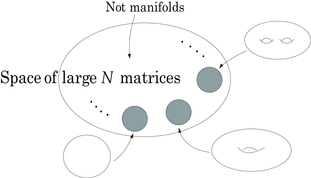
Figure 1: Path integral include all the curved spaces.

Classical solutions

Now let us consider the equation of motion. The action of IIB matrix model is given by Eq. (1). Variation with respect to $A_{a}$ gives the equation of motion

$$\left[A^{a},[A_{a},A_{b}]\right]=0.$$ (18)

Here, we simply set $\psi=0$. If we impose the ansatz

$$A_{a}=i\nabla_{(a)},$$ (19)

then Eq. (18) becomes

$$\left[\nabla^{(a)},\left[\nabla_{(a)},\nabla_{(b)}\right]\right]=0.$$ (20)

Equation (20) is equivalent to

$$0 = \left[\nabla^{a},\left[\nabla_{a},\nabla_{b}\right]\right]$$ (21)

$$= [\nabla^{a},R_{ab}{}^{cd}{\cal O}_{cd}]$$

$$= \left(\nabla^{a}R_{ab}{}^{cd}\right){\cal O}_{cd}-R_{b}{}^{c}\nabla_{c},$$

where $R_{ab}{}^{cd}$ is the Riemann tensor and $R_{b}{}^{c}=R_{ab}{}^{ac}$ is the Ricci tensor. Here we have assumed that $\nabla_{a}$ is torsionless. Note that Eq. (21) holds if and only if we have

$$\nabla^{a}R_{ab}{}^{cd}=0,\quad R_{ab}=0.$$ (22)

The first equation here follows from the second by the Bianchi identity $\nabla^{[a}R_{bc}{}^{de]}=0$. Therefore, the covariant derivative on a Ricci-flat spacetime is a classical solution.

We next consider a matrix model with a mass term:

$$S=-\frac{1}{g^{2}}tr\left(\frac{1}{4}[A_{a},A_{b}][A^{a},A^{b}]+\frac{1}{2}\bar{\psi}\gamma^{a}[A_{a},\psi]\right)+\frac{m^{2}}{g^{2}}tr\left(A_{a}A^{a}\right).$$ (23)

The equation of motion is now given by

$$[A_{b},[A_{a},A^{b}]]-2m^{2}A_{a}=0,$$ (24)

which leads to

$$R_{a}{}^{b}=-2m^{2}\delta_{a}{}^{b}.$$ (25)

This is the Einstein equation with a cosmological constant

$$\Lambda=-8m^{2}.$$ (26)

However, if $m^{2}>0$, the configuration $A_{a}=0\ (a=1,\cdots,10)$ is also a classical solution and has lower free energy. Therefore, such a configuration may dominate the path integral. If the positive mass term exists only for $d$ directions, $S_{{\rm mass}}=\frac{m^{2}}{g^{2}}\sum_{a=1}^{d}tr\left(A_{a}A^{a}\right)$, then we expect that these $d$ directions are collapsed to a point and the rest $10-d$ directions remain flat.

The analysis of the eigenvalue distribution [6] is consistent with this expectation. Suppose an effective mass term is generated in six directions and not in the rest four directions. Then that analysis indicates that the four dimensional spacetime is generated.

Diffeomorphism and local Lorentz invariance

We now show that the symmetries of general relativity are realized as parts of the $U(N)$ symmetry of the matrix model. The $U(N)$ symmetry of the matrix model is expressed as

$$\delta A_{a}=i[\Lambda,A_{a}],$$ (27)

where $\Lambda$ is a Hermitian matrix. If we expand $A_{a}$ as Eq. (17) and take

$$\Lambda=\frac{i}{2}\{\lambda^{(a)},\nabla_{(a)}\}=\frac{i}{2}\{\lambda^{a}(x),\nabla_{a}\},$$ (28)

Eq. (27) becomes a diffeomorphism on the fields that appear in Eq. (17), and $e_{a}{}^{m}$ and $\omega_{m}{}^{ab}$ that appear in $\nabla_{(a)}$. For example, we have

$$\delta e_{a}{}^{m}(x) = e_{a}{}^{n}(x)\nabla_{n}\lambda^{m}(x),$$ (29)

$$\delta\omega_{m}{}^{ab}(x) = \lambda^{n}(x)R_{mn}{}^{ab}(x),$$ (30)

$$\delta a_{a}(x) = -\lambda^{n}\nabla_{n}a_{a}(x).$$ (31)

This is the transformation law of the diffeomorphism. Similarly, if we take

$$\Lambda=i\lambda^{ab}(x){\cal O}_{ab},$$ (32)

we obtain

$$\delta e_{a}{}^{m}(x) = -\lambda_{a}{}^{b}(x)e_{b}{}^{m}(x),$$ (33)

$$\delta\omega_{m}{}^{ab}(x) = -\partial_{m}\lambda^{ab}(x)+2\lambda^{[a}{}_{c}(x)\omega_{m}{}^{b]c}(x),$$ (34)

which is the local Lorentz transformation.

3 Supercovariant derivative as a set of endomorphisms

In the last section we showed that the symmetries of general relativity can be embedded in the $U(N)$ symmetry of the matrix model. In order to implement local supersymmetry, we employ a superspace ${\cal M}$ as the base manifold and consider the supercovariant derivative.

3.1 General prescription

In this subsection, we introduce the supercovariant derivative on a $d$-dimensional ${\cal N}=1$ superspace and explain how to relate it to a set of endomorphisms.

The coordinates of the superspace are $z^{M}=(x^{m},\theta^{\mu})$, where $x^{m}\ (m=1,2,\cdots,d)$ are the bosonic components and $\theta^{\mu}\ (\mu=1,2,\cdots,d_{s})$ are the fermionic components. The quantity $d_{s}$ is the dimension of the spinor representation. For example, if $d=10$, $\theta$ corresponds to the Majorana-Weyl spinor and $d_{s}=16$. If $d=4$, $\theta$ corresponds to the Majorana spinor and $d_{s}=4$. Also, $M=(m,\mu)$ is an Einstein index, which can be converted into a Lorentz index, $A=(a,\alpha)$, using the supervielbein $E_{A}{}^{M}(x,\theta)$. In the following, we denote the Einstein indices by $M,N,L,\cdots$ and the Lorentz indices by $A,B,C,\cdots$.

The supercovariant derivative ${\nabla}$ which acts on Lorentz indices is defined as

$${\nabla}_{M}=\partial_{M}-\Omega_{M}{}^{ab}{\cal O}_{ab},$$ (35)

where $\partial_{M}=\left(\frac{\partial}{\partial x^{m}},\frac{\partial}{\partial\theta^{\mu}}\right)$ is the left-derivative and ${\cal O}_{ab}$ is the Lorentz generator. Note that ${\cal O}_{ab}$ has only Lorentz-vector indices. The action of $\nabla$ on an Einstein index is defined as follows:

$$\nabla_{M}V_{N} = (-)^{m(b+n)}E_{N}{}^{B}{\nabla}_{M}V_{B}$$ (36)

$$= \partial_{M}V_{N}+\Gamma_{MN}{}^{L}V_{L}.$$

Here, $m,n$ and $b$ are $0$ if $M,N$ and $B$ are bosonic indices and $1$ if they are fermionic indices. The quantity $\Gamma_{MN}{}^{L}$ is the Christoffel symbol, which is chosen to satisfy

$$\nabla_{M}E_{N}{}^{A}=0.$$ (37)

The commutation relation of ${\nabla}_{A}=E_{A}{}^{M}{\nabla}_{M}$ is given by

$$[{\nabla}_{A},{\nabla}_{B}\}=R_{AB}{}^{cd}{\cal O}_{cd}+T_{AB}{}^{C}{\nabla}_{C},$$ (38)

where $R_{AB}{}^{cd}$ is the super Riemann tensor and $T_{AB}{}^{C}$ is the supertorsion.

In §2.1, it is shown that the covariant derivative on a curved space can be expressed by a set of matrices. In the same way, the supercovariant derivative on a superspace can be expressed by a set of supermatrices.

Consider the principal $G=Spin(d)$ bundle ${\cal E}_{prin}$ over the superspace ${\cal M}$. If ${\cal M}=\cup_{i}{\cal U}_{i}$ is an open covering and $z_{[i]}=(x_{[i]},\theta_{[i]})$ and $z_{[j]}=(x_{[j]},\theta_{[j]})$ are the coordinates of the same point in ${\cal U}_{i}\cap{\cal U}_{j}$, then ${\cal E}_{prin}$ is constructed from ${\cal U}_{i}\times Spin(d)$ by identifying $(z_{[i]},g_{[i]})$ and $(z_{[j]},g_{[j]})$ in the case $g_{[i]}=t_{ij}(z)g_{[j]}$, where $t_{ij}(z)$ is the transition function. Taking $V=C^{\infty}({\cal E}_{prin})=\{f:{\cal E}_{prin}\to{\mathbb{C}}\}$, we can convert the Lorentz indices $a$ and $\alpha$ of the supercovariant derivatives into those with parentheses:

$${\nabla}_{(a)}=R_{(a)}{}^{b}(g^{-1}){\nabla}_{b},\quad{\nabla}_{(\alpha)}=R_{(\alpha)}{}^{\beta}(g^{-1}){\nabla}_{\beta}.$$ (39)

As in §2.1, the derivatives ${\nabla}_{(a)}$ and ${\nabla}_{(\alpha)}$ are globally defined on ${\cal E}_{prin}$ and, indeed, are endomorphisms on $C^{\infty}({\cal E}_{prin})$. The only difference between the two cases is that in the present case, transition functions, parameters of diffeomorphisms and local Lorentz transformations depend not only on the bosonic coordinates $x^{m}$ but also on the fermionic coordinates $\theta^{\mu}$. More specificality, ${\nabla}_{(a)}$ acts on $f\in V=C^{\infty}({\cal E}_{prin})$ as follows:

$${\nabla}_{(a)}^{[i]}f^{[i]}(z_{[i]},g_{[i]}) = R_{(a)}{}^{b}(g_{[i]}^{-1}){\nabla}_{b}^{[i]}f^{[i]}(z_{[i]},g_{[i]})$$ (40)

$$= R_{(a)}{}^{b}(g_{[i]}^{-1})R_{b}{}^{c}(t_{ij}(z)){\nabla}_{c}^{[j]}f^{[j]}(z_{[j]},g_{[j]})$$

$$= R_{(a)}{}^{c}((t_{ij}(z)^{-1}g_{[i]})^{-1}){\nabla}_{c}^{[j]}f^{[j]}(z_{[j]},g_{[j]})$$

$$= R_{(a)}{}^{c}(g_{[j]}^{-1}){\nabla}_{c}^{[j]}f^{[j]}(z_{[j]},g_{[j]})$$

$$= {\nabla}_{(a)}^{[j]}f^{[j]}(z_{[j]},g_{[j]}).$$

Similarly, we also have

$$\nabla_{(\alpha)}^{[i]}f^{[i]}(z_{[i]},g_{[i]})=\nabla_{(\alpha)}^{[j]}f^{[j]}(z_{[j]},g_{[j]}).$$ (41)

Therefore, the ${\nabla}_{(a)}$ and ${\nabla}_{(\alpha)}$ are endomorphisms on a supervector space $C^{\infty}({\cal E}_{prin})$, which are described by supermatrices, as we explain in the next section.

Before concluding this subsection, we give a proof that ${\nabla}_{(a)}$ and ${\nabla}_{(\alpha)}$ are anti-Hermitian and Hermitian, respectively. The standard inner product is defined by

$$\left(u(z,g),v(z,g)\right)=\int dg\int E\hskip 1.42271ptd^{d}x\hskip 1.42271ptd^{d_{s}}\theta\hskip 1.42271ptu^{\ast}(z,g)v(z,g),$$ (42)

where $dg$ is the Haar measure of $Spin(d)$ and $E=sdetE_{M}{}^{A}$. Then, we can show the (anti-) Hermiticity of $\nabla_{(A)}$ in the following way:

$$\left(u_{(a)}(z,g),{\nabla}^{(a)}v(z,g)\right) = \int E\hskip 1.42271ptd^{d}x\hskip 1.42271ptd^{d_{s}}\theta\hskip 1.42271ptu_{(a)}^{\ast}(z,g){\nabla}^{(a)}v(z,g)$$ (43)

$$= \int E\hskip 1.42271ptd^{d}x\hskip 1.42271ptd^{d_{s}}\theta\hskip 1.42271ptu_{a}^{\ast}(z,g){\nabla}^{a}v(z,g)$$

$$= -\int E\hskip 1.42271ptd^{d}x\hskip 1.42271ptd^{d_{s}}\theta\hskip 1.42271pt\left({\nabla}^{a}u_{a}^{\ast}(z,g)\right)v(z,g)$$

$$= -\int E\hskip 1.42271ptd^{d}x\hskip 1.42271ptd^{d_{s}}\theta\hskip 1.42271pt\left({\nabla}^{(a)}u_{(a)}^{\ast}(z,g)\right)v(z,g)$$

$$= -\left({\nabla}^{(a)}u_{(a)}(z,g),v(z,g)\right).$$

Similarly, we can show that

$$\left(u_{(\alpha)}(z,g),{\nabla}^{(\alpha)}v(z,g)\right)=\left({\nabla}^{(\alpha)}u_{(\alpha)}(z,g),v(z,g)\right).$$ (44)

The extra minus sign appears because $u^{\alpha}$ is fermionic.

The method presented in this subsection can be applied to a supersymmetry with any value of ${\cal N}$.

3.2 Example:two-dimensional ${\cal N}=(1,1)$ superspace

As a concrete example, let us construct a two-dimensional ${\cal N}=(1,1)$ superspace ${\cal M}$ with Lorentzian signature and a principal $Spin(1,1)$ bundle ${\cal E}_{prin}$ over it.

In order to eliminate the fields that are unnecessary in supergravity, we impose the following torsion constraints [7]:

$$T_{ab}{}^{c}=T_{\alpha\beta}{}^{\gamma}=0,\qquad T_{\alpha\beta}{}^{c}=2i(C\gamma^{c})_{\alpha\beta}.$$ (45)

Here $C_{\alpha\beta}$ is the charge-conjugation matrix. Let $M$ be the ordinary manifold which is obtained by setting all the fermionic coordinates $\theta$ of $M$ to zero. We denote by $e_{a}{}^{m}(x)$ and $\omega_{m}(x)=\omega_{m}{}^{01}(x)$ the zweibein on $M$ and the torsionless spin connection associated with $e_{a}{}^{m}(x)$, respectively. Then, using the higher-$\theta$ components of the superdiffeomorphism symmetry, we can write the superzweibein $E(x,\theta)$ and the spin connection $\Omega(x,\theta)$ in the form of the Wess-Zumino gauge [7]:

$$E_{M}{}^{A}(x,\theta) = \left(\begin{array}[]{cc}e_{m}{}^{a}(x)&-\frac{1}{2}\omega_{m}(x)(\gamma_{01}\theta)^{\alpha}\\ i(C\gamma^{a}\theta)_{\mu}&\delta_{\mu}{}^{\alpha}\end{array}\right),$$ (48)

$$E_{A}{}^{M}(x,\theta) = \left(\begin{array}[]{cc}e_{a}{}^{m}(x)&\frac{1}{2}\omega_{a}(x)(\gamma_{01}\theta)^{\mu}\\ -ie_{b}{}^{m}(x)(C\gamma^{b}\theta)_{\alpha}&\delta_{\alpha}{}^{\mu}-\frac{i}{4}(\bar{\theta}\theta)(\gamma_{01}\gamma^{b})^{\mu}{}_{\alpha}\omega_{b}(x)\end{array}\right),$$ (51)

$$\Omega_{m}{}^{01}(x,\theta)=\Omega_{m}(x,\theta)=\omega_{m}(x),\qquad\Omega_{\mu}^{01}(x,\theta)=\Omega_{\mu}(x,\theta)=0.$$ (52)

Here we have set the gravitino and auxiliary fields to zero for simplicity. The supercovariant derivative ${\nabla}_{A}=E_{A}{}^{M}{\nabla}_{M}$ is given by

$${\nabla}_{a}=E_{a}{}^{M}{\nabla}_{M}=e_{a}{}^{m}\partial_{m}-2\omega_{a}\left\{{\cal O}_{01}-\frac{1}{4}(\gamma_{01}\theta)^{\mu}\partial_{\mu}\right\},$$ (53)

$${\nabla}_{\alpha}=E_{\alpha}{}^{M}{\nabla}_{M}=\delta_{\alpha}{}^{\mu}\partial_{\mu}-i(C\gamma^{b}\theta)_{\alpha}{\nabla}_{b}.$$ (54)

Although ${\cal O}_{01}$ does not act on the index $\mu$, if we regard ${\cal O}_{01}-\frac{1}{4}(\gamma_{01}\theta)^{\mu}\partial_{\mu}$ as a “Lorentz generator”, it does act on $\mu$, and therefore $\theta^{\mu}$ can be regarded as a “Lorentz spinor”. Then ${\nabla}_{a}$ can be regarded as the ordinary covariant derivative on $M$ which also acts on the index $\mu$. In this sense, ${\cal M}$ is a spinor bundle over $M$ with Grassmann-odd fiber coordinates $\theta^{\mu}$, which is associated with the spin structure.

Now we introduce a principal $Spin(1,1)$ bundle ${\cal E}_{prin}$ over ${\cal M}$ associated with the spin structure. Then, we regard the supercovariant derivative ${\nabla}_{A}$ as acting on ${\cal E}_{prin}$. Parameterizing the spin $s$ representation of $Spin(1,1)$ as

$$R^{\langle s\rangle}(\varphi)=e^{2s\varphi},$$ (55)

we can express the Lorentz generator as

$${\cal O}_{01}=\frac{1}{4}\partial_{\varphi}.$$ (56)

Then, if we introduce $\theta^{(\mu)}$ according to the relation

$$\theta^{(\mu)}=(e^{\varphi\gamma_{01}})^{(\mu)}{}_{\nu}\theta^{\nu},$$ (57)

$\theta^{(\mu)}$ is globally defined on ${\cal E}_{prin}$. Next, using $x^{m},\theta^{(\mu)}$ and $\varphi$ as independent variables, we can rewrite Eqs. (53) and (54) as

$${\nabla}_{a} = e_{a}{}^{m}\left(\partial_{m}-\frac{1}{2}\omega_{m}\partial_{\varphi}\right),$$

$${\nabla}_{\alpha} = (e^{\varphi\gamma_{01}})^{(\mu)}{}_{\alpha}\partial_{(\mu)}-i(C\gamma^{b}e^{\varphi\gamma_{01}}\theta)_{\alpha}{\nabla}_{b}.$$ (58)

Finally, as explained in the previous subsection, we can convert indices without parentheses into those with parentheses, and hence we have

$${\nabla}_{(a)} = e_{(a)}{}^{m}\left(\partial_{m}-\frac{1}{2}\omega_{m}\partial_{\varphi}\right),$$ (59)

$${\nabla}_{(\alpha)} = \delta_{(\alpha)}{}^{(\mu)}\partial_{(\mu)}-i\left(C\gamma^{(b)}\theta\right)_{(\alpha)}{\nabla}_{(b)}.$$ (60)

Note that ${\cal E}_{prin}$ can be constructed as a direct product of ${\mathbb{R}}^{0|2}=\{\theta^{(1)},\theta^{(2)}\}$ and $E_{prin}$.

Supersphere

We now construct the homogeneous and isotropic Euclidean supersphere $S^{2|2}$ and the covariant derivative on it. Let us start with the case of the ordinary $S^{2}$ [1]. Then, by parameterizing $Spin(2)$ as

$$R^{\langle s\rangle}(\varphi)=e^{2is\varphi},\quad(\varphi\in[0,2\pi))$$ (61)

we can express the Lorentz generator in terms of the derivative with respect to $\varphi$ as

$${\cal O}_{+-}=\frac{1}{4i}\partial_{\varphi},$$ (62)

where $+$ and $-$ indicate the linear combinations of the Lorentz indices $1+i2$ and $1-i2$, respectively.

In the stereographic coordinates $(w,\bar{w})$ projected from the north pole, the metric is

$$g_{w\bar{w}}=g_{\bar{w}w}=\frac{1}{(1+w\bar{w})^{2}},\qquad g_{ww}=g_{\bar{w}\bar{w}}=0,$$ (63)

and we can take the zweibein and spin connection as

$$e_{+\bar{w}}=e_{-w}=\frac{1}{1+w\bar{w}},\quad e_{+w}=e_{-\bar{w}}=0,$$ (64)

$$\omega_{w}{}^{+-}=\frac{\bar{w}}{1+w\bar{w}},\quad\omega_{\bar{w}}{}^{+-}=-\frac{w}{1+w\bar{w}}.$$ (65)

Therefore, the covariant derivatives with parentheses are given by

$$\tilde{{\nabla}}_{(+)}^{[w]} = e^{-2i\varphi}\left((1+w\bar{w})\partial_{w}+\frac{i}{2}\bar{w}\partial_{\varphi}\right),$$

$$\tilde{{\nabla}}_{(-)}^{[w]} = e^{2i\varphi}\left((1+w\bar{w})\partial_{\bar{w}}-\frac{i}{2}w\partial_{\varphi}\right).$$ (66)

In the same way, in the stereographic coordinates $(w^{\prime},\bar{w}^{\prime})$ projected from the south pole, which are related to $(w,\bar{w})$ as $w^{\prime}=1/w$, we have

$$\tilde{{\nabla}}_{(+)}^{[w^{\prime}]} = e^{-2i\varphi^{\prime}}\left((1+w^{\prime}\bar{w}^{\prime})\partial_{w^{\prime}}+\frac{i}{2}\bar{w}^{\prime}\partial_{\varphi^{\prime}}\right),$$

$$\tilde{{\nabla}}_{(-)}^{[w^{\prime}]} = e^{2i\varphi^{\prime}}\left((1+w^{\prime}\bar{w}^{\prime})\partial_{\bar{w}^{\prime}}-\frac{i}{2}w^{\prime}\partial_{\varphi^{\prime}}\right).$$ (67)

Here, the coordinate $\varphi^{\prime}$ of the fiber on this patch is related to $\varphi$ according to the transition function

$$\varphi^{\prime}=\varphi+\arg(w)+\frac{\pi}{2}.$$ (68)

We can explicitly check that Eqs. (66) and (67) are identical. Note that $E_{prin}$ on $S^{2}$ is $Spin(2)(=S^{1})$ bundle over $S^{2}$ and is topologically $S^{3}$.

Next we consider the supersphere $S^{2|2}$ and the principal $Spin(2)$ bundle ${\cal E}_{prin}$ over it. In this case Eqs. (59) and (60) become

$${\nabla}_{(+)}^{[w]} = e^{-2i\varphi}\left\{(1+w\bar{w})\partial_{w}+\frac{i}{2}\bar{w}\partial_{\varphi}\right\},$$

$${\nabla}_{(-)}^{[w]} = e^{2i\varphi}\left\{(1+w\bar{w})\partial_{\bar{w}}-\frac{i}{2}w\partial_{\varphi}\right\},$$ (69)

$${\nabla}_{(\alpha)}^{[w]} = \delta_{(\alpha)}{}^{(\mu)}\partial_{(\mu)}-i\left(C\gamma^{(b)}\theta\right)_{(\alpha)}{\nabla}_{(b)}.$$ (70)

Using the relation $(w,\theta_{[w]}^{(\mu)})=(1/w^{\prime},\theta_{[w^{\prime}]}^{(\mu)})$ and Eq. (68), we can explicitly confirm the relation

$${\nabla}_{(A)}^{[w]}={\nabla}_{(A)}^{[w^{\prime}]}.$$ (71)

In this way, we can describe the supersphere $S^{2|2}$ in terms of four supermatrices.

4 Supermatrix model and local supersymmetry

In the previous section, we showed that the supercovariant derivative on a superspace can be described by a set of supermatrices. Therefore, as in §2.2, we can embed local supersymmetry manifestly in supermatrix models. In this section, we consider a straightforward generalization of IIB matrix model. We show that the equation of motion of the supermatrix model is compatible with that of supergravity.

4.1 Supermatrix model

An element $f:{\cal E}_{prin}\to{\mathbb{C}}$ of $V=C^{\infty}({\cal E}_{prin})$ can be expressed as a power series in $\theta^{\mu}$. The coefficients of even powers of $\theta^{\mu}$ in this series are Grassmann-even functions and form the Grassmann-even subspace $V_{e}$ of $V$. Similarly, the coefficients of odd powers of $\theta^{\mu}$ form the Grassmann-odd subspace $V_{o}$. Therefore, the total space $V$ is the direct sum of $V_{e}$ and $V_{o}$:

$$V=V_{e}\oplus V_{o}.$$ (72)

If we introduce a regularization of $V$ in which the dimensions of $V_{e}$ and $V_{o}$ are $N_{e}$ and $N_{o}$, respectively, then a linear transformation on $V$ can be expressed as a $(N_{e},N_{o})$-supermatrix. We summarize the definition and properties of supermatrix in Appendix A.

The derivatives ${\nabla}_{(a)}$ and ${\cal O}_{ab}$ map an even (resp., odd) element to an even (resp., odd) element. Hence they can be expressed in terms of even supermatrices. Contrastingly, ${\nabla}_{(\alpha)}$ maps an even element to an odd element and vice versa. Therefore they are expressed in terms of odd supermatrices.

Now we propose the supermatrix generalization of IIB matrix model. The dynamical variables consist of Hermitian even supermatrices ${\cal A}_{a}$ with vector indices and the Hermitian odd supermatrices $\Psi_{\alpha}$ with spinor indices. The action is given by

$$S=-\frac{1}{g^{2}}Str\left(\frac{1}{4}[{\cal A}_{a},{\cal A}_{b}][{\cal A}^{a},{\cal A}^{b}]+\frac{1}{2}\bar{\Psi}^{\alpha}\left(\gamma^{a}\right)_{\alpha}{}^{\beta}[{\cal A}_{a},\Psi_{\beta}]\right).$$ (73)

This model possesses superunitary symmetry $U(N_{e}|N_{o})$. If the matrices ${\cal A}_{a}$ are sufficiently close to the covariant derivatives $i{\nabla}_{(a)}$ on some ${\cal E}_{prin}$, we regard the $A_{a}$ and $\Psi_{\alpha}$ as endomorphisms of $V=C^{\infty}({\cal E}_{prin})$. As we discuss in the next section, there is a possibility that Eq. (73) is equivalent to the original IIB matrix model.

A remark on the role of the odd supermatrix $\Psi_{\alpha}$ is in order here. The action (73) has the global symmetry

$$\delta^{(1)}{\cal A}_{a}=-i\overline{\Psi}\gamma_{a}\hat{\epsilon},\qquad\delta^{(1)}\Psi_{\alpha}=\frac{i}{2}\left[{\cal A}_{a},{\cal A}_{b}\right]\left(\gamma^{ab}\hat{\epsilon}\right)_{\alpha}$$ (74)

and

$$\delta^{(2)}{\cal A}_{a}=0,\qquad\delta^{(2)}\Psi_{\alpha}=\hat{\epsilon}_{\alpha},$$ (75)

which is the analogue of the ${\cal N}=2$ global supersymmetry of the original IIB matrix model. Here, the quantities

$$\hskip 48.36958pt\overset{N_{e}}{\rotatebox{90.0}{\}}}\hskip 9.95863pt\overset{N_{o}}{\rotatebox{90.0}{\}}}$$

$$\hat{\epsilon}_{\alpha}=\epsilon_{\alpha}\left(\begin{array}[]{cc}1&0\\ 0&-1\end{array}\right)\begin{array}[]{c}{\scriptstyle\}N_{e}}\\ {\scriptstyle\}N_{o}}\end{array}$$ (80)

are odd scalar supermatrices, which commute with ${\cal A}_{a}$ and anticommute with $\Psi_{\alpha}$. In the original interpretation of IIB matrix model, this symmetry is simply the ten-dimensional ${\cal N}=2$ supersymmetry. In the case of the supermatrix model, however, the local supersymmetry is manifestly embedded as a part of the superunitary symmetry, as we see in §4.3. Indeed, a supermatrix model without $\Psi_{\alpha}$, such as

$$S=-\frac{1}{4g^{2}}Str\left([{\cal A}_{a},{\cal A}_{b}][{\cal A}^{a},{\cal A}^{b}]\right),$$ (81)

also possesses this local supersymmetry. Furthermore, as we see in the next subsection, both Eqs. (73) and (81) describe supergravity at the level of classical solutions. On the other hand, in the original interpretation of IIB matrix model, in which matrices are regarded as coordinates, the ${\cal N}=2$ global supersymmetry prevents the eigenvalues from collapsing to one point, and this allows a reasonable interpretation of spacetime [3]. We conjecture that the global symmetry represented by Eqs. (74) and (75) plays a similar role here and allows ${\cal A}_{a}$ to fluctuate around $i\nabla_{(a)}$ on some manifold.

4.2 Classical solutions

In this subsection we investigate classical solutions of Eq. (73). For simplicity, let us consider the four-dimensional model here. We use the notation of Ref. WZ77. In this case, ${\cal A}_{a}$ and $\Psi_{\alpha}$ are four-dimensional vector and Majorana spinor, respectively. The equations of motion are given by

$$[{\cal A}^{a},[{\cal A}_{a},{\cal A}_{b}]]+(C\gamma_{b})^{\alpha\beta}\{\Psi_{\alpha},\Psi_{\beta}\}=0,$$ (82)

$$(\gamma^{a})_{\alpha}{}^{\beta}[{\cal A}_{a},\Psi_{\beta}]=0,$$ (83)

where $C^{\alpha\beta}$ is the charge-conjugation matrix.

We impose the following ansatz:

$${\cal A}_{a}=i{\nabla}_{(a)},\qquad\Psi_{\alpha}=0.$$ (84)

In the bosonic case, once we impose the ansatz (19), we can obtain the general solution of the matrix equation of motion (18). In the present case, however, it is not easy to find the general solution of Eqs. (82) and (83). Instead, we show that the ansatz (84) satisfies Eqs. (82) and (83) if we impose the standard off-shell torsion constraints [10, 9]

$$T_{\alpha\beta}{}^{c} = 2i(\gamma^{c}C^{-1})_{\alpha\beta},$$

$$T_{\alpha\beta}{}^{\gamma} = 0,$$

$$T_{a\beta}{}^{c} = 0,$$

$$T_{ab}{}^{c} = 0,$$ (85)

and the equation of motion of supergravity [10],

$$T_{a\beta}{}^{\gamma} = 0.$$ (86)

Using Eqs. (85) and (86), we have

$$[{\nabla}^{a},[{\nabla}_{a},{\nabla}_{b}]] = [{\nabla}^{a},R_{ab}{}^{cd}{\cal O}_{cd}+T_{ab}{}^{\gamma}{\nabla}_{\gamma}]$$ (87)

$$= ({\nabla}^{a}R_{ab}{}^{cd}){\cal O}_{cd}-R_{ab}{}^{ac}{\nabla}_{c}+({\nabla}^{a}T_{ab}{}^{\gamma}){\nabla}_{\gamma}+T_{ab}{}^{\gamma}R^{a}{}_{\gamma}{}^{cd}{\cal O}_{cd}.$$

Furthermore, as shown in Appendix B, from Eqs. (85), (86) and the Bianchi identities, we can show the relations

$$R_{ab}{}^{ac} = 0,$$ (88)

$${\nabla}^{a}T_{ab}{}^{\gamma} = 0,$$ (89)

$${\nabla}^{a}R_{ab}{}^{cd} = 0,$$ (90)

$$T_{ab}{}^{\gamma}R^{a}{}_{\gamma}{}^{cd} = 0,$$ (91)

which indicate that the right-hand side of Eq. (87) is zero. Hence, the ansatz (84) with the constraints (85) and (86) satisfies Eqs. (82) and (83).

Some comments are in order here. First, although we showed that Eqs. (85) and (86) are sufficient conditions for Eqs. (82) and (83) under the assumption (84), it is unclear whether or not they are necessary. Secondly, it is desirable to determine whether the torsion constraints in the ten-dimensional superspace [14] are compatible with the equation of motion of the supermatrix model. Thirdly, because we have set $\Psi_{\alpha}$ to zero as an ansatz, the action (81) allows the same classical solutions.

4.3 Superdiffeomorphism and local supersymmetry

The supermatrix model possesses the superunitary symmetry

$$\delta{\cal A}_{a}=i[\Lambda,{\cal A}_{a}],\quad\delta\Psi_{\alpha}=i[\Lambda,\Psi_{\alpha}],$$ (92)

where $\Lambda$ is an even Hermitian supermatrix. If we expand ${\cal A}_{a}$ and $\Psi_{\alpha}$ as

$${\cal A}_{a} = i{\nabla}_{(a)}+a_{(a)}(z,g)+ia_{(a)}{}^{(B)}(z,g){\nabla}_{(B)}+ia_{(a)}{}^{bc}(z,g){\cal O}_{bc}$$

$$\quad+i^{2}a_{(a)}{}^{(B)(C)}(z,g){\nabla}_{(B)}{\nabla}_{(C)}+i^{2}a_{(a)}{}^{(B),cd}(z,g){\nabla}_{(B)}{\cal O}_{cd}+\cdots,$$

$$\Psi_{\alpha} = \psi_{(\alpha)}(z,g)+i\psi_{(\alpha)}{}^{(B)}(z,g){\nabla}_{(B)}+i\psi_{(\alpha)}{}^{bc}(z,g){\cal O}_{bc}$$

$$\quad+i^{2}\psi_{(\alpha)}{}^{(B)(C)}(z,g){\nabla}_{(B)}{\nabla}_{(C)}+i^{2}\psi_{(\alpha)}{}^{(B),cd}(z,g){\nabla}_{(B)}{\cal O}_{cd}+\cdots,$$

$${\nabla}_{(A)} = E_{(A)}{}^{M}{\nabla}_{M},$$ (93)

and take $\Lambda$ as

$$\Lambda=\frac{i}{2}\left\{\lambda^{(a)}(z),{\nabla}_{(a)}\right\}+\frac{i}{2}\left[\lambda^{(\alpha)}(z),{\nabla}_{(\alpha)}\right],$$ (94)

then Eq. (92) becomes a superdiffeomorphism on the fields that appear in Eq. (93).

The part of the superdiffeomorphism generated by

$$\Lambda=\frac{i}{2}\left[\lambda^{(\alpha)}(x),{\nabla}_{(\alpha)}\right]$$ (95)

gives the local supersymmetry. For example, in the Wess-Zumino gauge [8, 9]

$$\left.E_{M}{}^{A}\right|_{\theta=0}=\left(\begin{array}[]{cc}e_{m}{}^{a}(x)&\frac{1}{2}\chi_{m}{}^{\alpha}(x)\\ 0&\delta_{\mu}{}^{\alpha}\end{array}\right),$$ (98)

where $e_{m}{}^{a}$ is the vielbein and $\chi_{m}{}^{\alpha}$ is the gravitino, Eq. (95) gives

$$\delta e_{m}{}^{a}(x)=2i\bar{\lambda}(x)\gamma^{a}\chi_{\mu}(x),\qquad\delta\chi_{m}{}^{\alpha}(x)=2{\nabla}_{m}\lambda^{\alpha}(x)+({\rm auxiliary\ fields}).$$ (99)

5 Conclusions and discussion

In Ref. HKK we showed that the covariant derivative on a $d$-dimensional curved space can be described by a set of $d$ matrices. Based on this, we introduced a new interpretation of the matrix model, in which we regard matrices as covariant derivatives on a curved space rather than coordinates. With this interpretation, the symmetries of general relativity are included in the unitary symmetry of the matrix model, and the path integral contains a summation over all curved spaces. In this paper, we have extended this formalism to include supergravity. If we promote matrices to supermatrices, we can express supercovariant derivatives as special configurations of the supermatrices. Then, the local supersymmetry is included in the superunitary symmetry. Furthermore, we showed that if we consider the action $S=-Str\left[{\cal A}_{a},{\cal A}_{b}\right]^{2}+\cdots$, the matrix equation of motion follows from the Einstein and the Rarita-Schwinger equations in the four-dimensional case.

There remain several problems. First, it is desirable to clarify the relationship between our new interpretation and the original one, in which matrices represent coordinates. Although gravity is realized manifestly in the new interpretation, its relationship to string theory is rather obscure. Contrastingly, the original interpretation is directly connected to string theory, because the action can be regarded as the Green-Schwarz action of a type-IIB superstring. Furthermore, we have not understood the meaning of the global ${\cal N}=2$ supersymmetry of IIB matrix model in the new interpretation. Because we have realized supersymmetry as superunitary symmetry, it seems that global ${\cal N}=2$ supersymmetry need not exist. In the original IIB matrix model, however, it prevents the eigenvalues from collapsing to a point and allows a reasonable interpretation of spacetime [3]. We believe that in the new interpretation it plays a similar role and allows ${\cal A}_{a}$ to fluctuate around a covariant derivative on some manifold. In order to connect the two different interpretations, it may be helpful to consider noncommutative geometry. This is because there is no essential difference between coordinates and derivatives in noncommutative geometry [13]. If we can understand the relationship more closely, the role of the global ${\cal N}=2$ supersymmetry may become clear. Furthermore, this would be useful for the construction of curved noncommutative manifolds.

Secondly, it remains to investigate whether ten-dimensional supergravity can be derived from the equation of motion of our supermatrix model. In Refs. ADR, the superspace formulation of ten-dimensional ${\cal N}=1$ supergravity coupled to super Yang-Mills was studied, and the torsion constraints were presented. The calculation in the ten-dimensional case is more complicated, due to the presence of various fields, including the dilaton, antisymmetric tensor and gauge field. At present, it is unclear whether the torsion constraints presented in Refs. ADR fit our supermatrix model. If they do not, we may need to modify the form of the action or to find other torsion constraints.

Thirdly, the supermatrix model we have proposed might not be well-defined, because the action is not bounded from below, due to the minus sign appearing in the supertrace. The possibility that supermatrix models are formally equivalent to the corresponding ordinary matrix models is discussed in Refs. Alvarez-Gaume and OT. If a similar mechanism holds in our supermatrix model, we may be able to embed supergravity in the original IIB matrix model.

Appendix A Supermatrices

In this appendix we define a supermatrix and summarize its properties.

Consider a supervector space $V$. We use the standard basis in which supervectors have the form

$$v=\left(\begin{array}[]{c}v_{1}\\ v_{2}\end{array}\right)\begin{array}[]{c}{\scriptstyle\}N_{e}}\\ {\scriptstyle\}N_{o}}\end{array},$$ (A.5)

where $v_{1}$ and $v_{2}$ are bosonic and fermionic column vectors, respectively. We call $v$ an even supervector. Multiplying $v$ by a Grassmann-odd number, we obtain an odd supervector.

In the standard basis defined above, an even supermatrix ${\cal B}$ and an odd supermatrix ${\cal F}$ can be written as

$$\hskip 36.98866pt\overset{N_{e}}{\rotatebox{90.0}{\}}}\hskip 14.22636pt\overset{N_{o}}{\rotatebox{90.0}{\}}}\hskip 109.54327pt\overset{N_{e}}{\rotatebox{90.0}{\}}}\hskip 14.22636pt\overset{N_{o}}{\rotatebox{90.0}{\}}}$$

$${\cal B}=\left(\begin{array}[]{cc}B_{1}&F_{1}\\ F_{2}&B_{2}\end{array}\right)\begin{array}[]{c}{\scriptstyle\}N_{e}}\\ {\scriptstyle\}N_{o}}\end{array},\qquad{\cal F}=\left(\begin{array}[]{cc}F_{1}^{\prime}&B_{1}^{\prime}\\ B_{2}^{\prime}&F_{2}^{\prime}\end{array}\right)\begin{array}[]{c}{\scriptstyle\}N_{e}}\\ {\scriptstyle\}N_{o}}\end{array}.$$ (A.14)

Here $B$ and $B^{\prime}$ are bosonic matrices and $F$ and $F^{\prime}$ are fermionic matrices. An even supermatrix represents a linear transformation of the supervectorspace $V$, which maps an even (resp., odd) supervector to an even (resp., odd) supervector. An odd supermatrix also represents a linear transformation of $V$, but it maps an even (resp., odd) supervector to an odd (resp., even) supervector.

A scalar supermatrix is defined by

$$\hskip 38.41139pt\overset{N_{e}}{\rotatebox{90.0}{\}}}\hskip 5.40608pt\overset{N_{o}}{\rotatebox{90.0}{\}}}\hskip 105.2751pt\overset{N_{e}}{\rotatebox{90.0}{\}}}\hskip 8.5359pt\overset{N_{o}}{\rotatebox{90.0}{\}}}$$

$$\hat{c}=c\left(\begin{array}[]{cc}1&0\\ 0&1\end{array}\right)\begin{array}[]{c}{\scriptstyle\}N_{e}}\\ {\scriptstyle\}N_{o}}\end{array},\qquad\hat{\epsilon}=\epsilon\left(\begin{array}[]{cc}1&0\\ 0&-1\end{array}\right)\begin{array}[]{c}{\scriptstyle\}N_{e}}\\ {\scriptstyle\}N_{o}}\end{array},$$ (A.23)

where $c$ and $\epsilon$ are Grassmann-even and odd numbers. Then, $\hat{c}$ commutes with both even and odd supermatrices, and $\hat{\epsilon}$ commutes (resp., anticommutes) with an even (resp., odd) supermatrix.

The Hermitian conjugate is defined by

$${\cal B}^{\dagger}=\left(\begin{array}[]{cc}B_{1}^{\dagger}&F_{2}^{\dagger}\\ F_{1}^{\dagger}&B_{2}^{\dagger}\end{array}\right),\qquad{\cal F}^{\dagger}=\left(\begin{array}[]{cc}F_{1}^{\prime\dagger}&B_{2}^{\prime\dagger}\\ B_{1}^{\prime\dagger}&F_{2}^{\prime\dagger}\end{array}\right).$$ (A.28)

A supermatrix ${\cal S}$ is Hermitian if ${\cal S}^{\dagger}={\cal S}$. Then, Hermitian matrices can be written as

$${\cal B}=\left(\begin{array}[]{cc}B_{1}&F\\ F^{\dagger}&B_{2}\end{array}\right),\qquad{\cal F}=\left(\begin{array}[]{cc}F_{1}&B\\ B^{\dagger}&F_{2}\end{array}\right),\qquad$$ (A.33)

where $B_{i}$ and $F_{i}$ are bosonic and fermionic Hermitian matrices, and $B$ and $F$ are bosonic and fermionic complex matrices.

The supertrace is defined by

$$Str\ {\cal B}=Str\left(\begin{array}[]{cc}B_{1}&F_{1}\\ F_{2}&B_{2}\end{array}\right)=tr\ B_{1}-tr\ B_{2},$$ (A.36)

$$Str\ {\cal F}=Str\left(\begin{array}[]{cc}F_{1}^{\prime}&B_{1}^{\prime}\\ B_{2}^{\prime}&F_{2}^{\prime}\end{array}\right)=tr\ F_{1}^{\prime}+tr\ F_{2}^{\prime}.$$ (A.39)

It satisfies the cyclicity relation

$$Str\left({\cal S}_{1}{\cal S}_{2}\right)=(-)^{s_{1}s_{2}}Str\left({\cal S}_{2}{\cal S}_{1}\right),$$ (A.40)

where $s_{i}$ is $0$ (resp., $1$) if ${\cal S}_{i}$ is even (resp., odd). It also satisfies the following property for scalar supermatrices $\hat{c}$ and $\hat{\epsilon}$:

$$Str\left(\hat{c}{\cal S}\right)=c\cdot Str\ {\cal S},\qquad Str\left(\hat{\epsilon}{\cal S}\right)=\epsilon\cdot Str\ {\cal S}.$$ (A.41)

Finally, the superdeterminant is defined for even supermatrices by

$$sdet{\cal B}=\exp\left(Str\log{\cal B}\right).$$ (A.42)

Appendix B Derivation of Eqs. (88), (89), (90) and (91) from Eqs. (85) and (86)

In this appendix we show that if the torsion constraints and equations of motion of the four-dimensional supergravity in superspace, Eqs. (85) and (86), are satisfied, then Eqs. (88), (89) and (90), and hence the equations of motion of the matrix model, are satisfied. The argument is almost parallel to that given in Ref. WZ77.

B.1 Bianchi identities

The supertorsion and the super Riemann tensor satisfy the following Bianchi identities which arise from the super Jacobi identities. If we use Eqs. (85) and (86) to simplify the Bianchi identities,
$[{\nabla}_{a},[{\nabla}_{b},{\nabla}_{c}]]+({\rm cyclic})=0$ gives

$$R_{[abc]}{}^{i}=0,$$ (B.1)

$${\nabla}_{[a}R_{bc]}{}^{ij}+T_{[ab}{}^{\gamma}R_{c]\gamma}{}^{ij}=0,$$ (B.2)

$[{\nabla}_{a},[{\nabla}_{b},{\nabla}_{\gamma}]]+({\rm cyclic})=0$ gives

$$-R_{b\gamma a}{}^{i}+R_{a\gamma b}{}^{i}-2iT_{ab}{}^{\delta}\left(\gamma^{i}\right)_{\gamma\delta}=0,$$ (B.3)

$$\frac{1}{4}R_{ab}{}^{ij}\left(\gamma_{ij}\right)_{\gamma}{}^{\delta}-{\nabla}_{\gamma}T_{ab}{}^{\delta}=0,$$ (B.4)

and $[{\nabla}_{a},\{{\nabla}_{\beta},{\nabla}_{\gamma}\}]+\{{\nabla}_{\beta},[{\nabla}_{\gamma},{\nabla}_{a}]\}-\{{\nabla}_{\gamma},[{\nabla}_{a},{\nabla}_{\beta}]\}=0$ gives

$$R_{\beta\gamma}{}^{ij}=0,$$ (B.5)

$$2i\left(\gamma^{k}\right)_{\beta\gamma}R_{ak}{}^{ij}-{\nabla}_{\beta}R_{a\gamma}{}^{ij}-{\nabla}_{\gamma}R_{a\beta}{}^{ij}=0,$$ (B.6)

$$2i\left(\gamma^{k}\right)_{\beta\gamma}T_{ak}{}^{\delta}-\frac{1}{4}R_{a\gamma}{}^{ij}\left(\gamma_{ij}\right)_{\beta}{}^{\delta}-\frac{1}{4}R_{a\beta}{}^{ij}\left(\gamma_{ij}\right)_{\gamma}{}^{\delta}=0,$$ (B.7)

where we have used Eq. (B.5) to simplify Eq. (B.6). Here we have presented only the identities that we need in the following.

B.2 Derivation of Eqs. (88), (89) and (90)

B.2.1 Proof of $R_{ab}{}^{cd}=R^{cd}{}_{ab}$

From the fact that $R_{ab}{}^{cd}$ is antisymmetric under the exchanges $a\leftrightarrow b$ and $c\leftrightarrow d$ and Eq. (B.1), it follows that

$$R_{abcd} = -R_{bcad}-R_{cabd}$$ (B.8)

$$= -R_{cbda}+R_{cadb}$$

$$= R_{dcba}+R_{bdca}-R_{adcb}-R_{dcab}$$

$$= 2R_{cdab}+R_{dbac}+R_{adbc}$$

$$= 2R_{cdab}-R_{badc}$$

$$= 2R_{cdab}-R_{abcd}.$$

Hence, we have

$$R_{ab}{}^{cd}=R^{cd}{}_{ab}.$$ (B.9)

B.2.2 Proof of the Rarita-Schwinger equation

Multiplying Eq. (B.7) by $\frac{1}{4}(\gamma_{b})^{\gamma\beta}$, we have

$$2iT_{ab}{}^{\delta} = \frac{1}{8}R_{a\beta}{}^{ij}(\gamma_{b}\gamma_{ij})^{\beta\delta}$$ (B.10)

$$= \frac{1}{8}R_{a\beta}{}^{ij}\left(\eta_{bi}\gamma_{j}-\eta_{bj}\gamma_{i}+\gamma_{bij}\right)^{\beta\delta}$$

$$= \frac{1}{4}R_{a\beta b}{}^{j}(\gamma_{j})^{\beta\delta}+\frac{1}{8}R_{a\beta}{}^{ij}(\gamma_{bij})^{\beta\delta}$$

$$= \frac{1}{4}R_{a\beta b}{}^{j}(\gamma_{j})^{\delta\beta}-\frac{1}{8}R_{a\beta}{}^{ij}(\gamma_{bij})^{\delta\beta}.$$

Then, multiplying this by $(\gamma^{b})^{\gamma}{}_{\delta}$, we obtain

$$2i(\gamma^{b})^{\gamma}{}_{\delta}T_{ab}{}^{\delta} = \frac{1}{4}R_{a\beta}{}^{bj}(\gamma_{bj})^{\gamma\beta}-\frac{1}{8}R_{a\beta}{}^{ij}(\gamma^{b}\gamma_{bij})^{\gamma\beta}$$ (B.11)

$$= \frac{1}{4}R_{a\beta}{}^{ij}(\gamma_{ij})^{\gamma\beta}-\frac{4-2}{8}R_{a\beta}{}^{ij}(\gamma_{ij})^{\gamma\beta}$$

$$= 0.$$

On the other hand, by contracting $\gamma$ and $\delta$ in (B.7), we have

$$2i(\gamma^{b})^{\gamma}{}_{\delta}T_{ab}{}^{\delta}=\frac{1}{4}R_{a\beta}{}^{ij}(\gamma_{ij})^{\gamma\beta}.$$ (B.12)

Therefore, we find

$$(\gamma^{a})_{\alpha\beta}T_{ab}{}^{\beta}=0,\qquad R_{a\beta}{}^{ij}(\gamma_{ij})^{\gamma\beta}=0.$$ (B.13)

The former is the Rarita-Schwinger equation written in terms of superspace [8].

B.2.3 Proof of the Einstein equation (88)

By contracting $a$ and $i$ in Eq. (B.3) and using the second equation in Eq. (B.13), we find that

$$R_{a\gamma}{}^{ac}=0.$$ (B.14)

Next, contracting $a$ and $i$ in Eq. (B.6) and substituting the above equation, we obtain

$$(\gamma^{k})_{\beta\gamma}R_{ak}{}^{aj}=0,$$ (B.15)

which is equivalent to Eq. (88):

$$R_{ab}{}^{ac}=0.$$ (B.16)

This is the Einstein equation without a cosmological constant. Note that the super Ricci tensor $R_{ab}{}^{ac}$ contains the contribution from the energy-momentum of the gravitino.

B.2.4 Proof of Eq. (89)

By Eqs. (85) and (B.5), we have

$$\{{\nabla}_{\alpha},{\nabla}_{\beta}\} = 2i(\gamma^{a}C^{-1})_{\alpha\beta}{\nabla}_{a}\ ,$$ (B.17)

$${\nabla}_{a} = -\frac{i}{8}\left(C\gamma_{a}\right)^{\alpha\beta}\{{\nabla}_{\alpha},{\nabla}_{\beta}\}$$ (B.18)

$$= -\frac{i}{8}\left(C\gamma_{a}\right)^{\alpha\beta}{\nabla}_{\alpha}{\nabla}_{\beta}\ .$$

Then, multiplying Eq. (B.4) by $(\gamma^{a})_{\rho}{}^{\gamma}$, we have

$$(\gamma^{a})_{\rho}{}^{\gamma}{\nabla}_{\gamma}T_{ab}{}^{\delta} = \frac{1}{4}(\gamma^{a}\gamma^{ij})_{\rho}{}^{\delta}R_{abij}$$ (B.19)

$$= \frac{1}{4}\left(\gamma^{aij}+\eta^{ai}\gamma^{j}-\eta^{aj}\gamma^{i}\right)_{\rho}{}^{\delta}R_{abij}$$

$$= 0.$$

Here we have used the relation $R_{a[bcd]}=0$, which follows from Eqs. (B.9) and (B.1), and Eq. (B.16). Next, multiplying Eq. (B.19) by ${\nabla}^{\rho}$ and using Eq. (B.18), we obtain Eq. (89):

$${\nabla}^{a}T_{ab}{}^{\delta}=0.$$ (B.20)

B.2.5 Proof of Eqs. (90) and (91)

From Eqs. (B.13), (B.3) and (B.7), it follows that [8, 9]

$$R_{\alpha b}{}^{cd}=2i(\gamma_{b}C^{-1})_{\alpha\beta}T^{cd\beta}.$$ (B.21)

Then, because $C\gamma^{a}$ is symmetric, we have

$$T_{bc}{}^{\gamma}R^{a}{}_{\gamma}{}^{ij}=T^{ij\gamma}R^{a}{}_{\gamma}{}_{bc}.$$ (B.22)

Combining this with Eq. (B.9), we can rewrite Eq. (B.2) as

$${\nabla}^{[a}R_{ij}{}^{bc]}+T_{ij}{}^{\gamma}R^{[a}{}_{\gamma}{}^{bc]}=0.$$ (B.23)

The second term on the right-hand side is zero, because substituting Eq. (B.21) into Eq. (B.3) we have $R^{[a}{}_{\gamma}{}^{bc]}=0$. Therefore, we obtain

$${\nabla}^{[a}R_{ij}{}^{bc]}=0,$$ (B.24)

and contracting $a$ and $i$, we have

$${\nabla}^{a}R_{ab}{}^{cd}+{\nabla}^{c}R_{ab}{}^{da}+{\nabla}^{d}R_{ab}{}^{ac}=0.$$ (B.25)

Because the second and third terms are zero, by Eq. (B.16), we obtain Eq. (90):

$${\nabla}^{a}R_{ab}{}^{cd}=0\ .$$ (B.26)

From Eq. (B.21) we have

$$T_{ab}{}^{\gamma}R^{a}{}_{\gamma}{}^{ij} = T_{ab}{}^{\gamma}\cdot(-2i)(\gamma^{a}C^{-1})_{\gamma\delta}T^{ij\delta}$$ (B.27)

$$= 2iT^{ij\delta}\cdot(\gamma^{a}C^{-1})_{\delta\gamma}T_{ab}{}^{\gamma},$$

but this is zero, by Eq. (B.13). Therefore, we have shown Eq. (91).

Appendix C Proof of $\kappa=0$

In the footnote of §4.2, we claimed that if we stipulate ${\cal A}_{a}=i{\nabla}_{(a)},\ \Psi_{\alpha}=\kappa{\nabla}_{(\alpha)}$ and the standard off-shell torsion constraints (85) as an ansatz, then the equations of motion (82) and (83) of the matrix model force $\kappa$ to be zero. In this appendix, we give an outline of its proof.

By combining Eq. (85) with the Bianchi identities, the remaining degrees of freedoms can be expressed in terms of three superfields: the complex scalar $R$, the real vector $G_{a}$, and the spin $\frac{3}{2}$ field $W_{(\alpha\beta\gamma)}$ [12, 9].

If $\kappa\neq 0$, Eq. (83) reduces to

$$(\gamma^{a})_{\alpha}{}^{\beta}\left(R_{a\beta}{}^{cd}{\cal O}_{cd}+T_{a\beta}{}^{\gamma}{\nabla}_{\gamma}\right)=0,$$ (C.1)

which is equivalent to

$$(\gamma^{a})_{\alpha}{}^{\beta}R_{a\beta}{}^{cd} = 0,$$ (C.2)

$$(\gamma^{a})_{\alpha}{}^{\beta}T_{a\beta}{}^{\gamma} = 0.$$ (C.3)

In terms of $G,R$ and $W$, the latter becomes

$$G_{a}=R=0.$$ (C.4)

This is the equation of motion of supergravity [10], and it is equivalent to Eq. (86). As explained in the previous subsection, this implies Eq. (B.16); that is, the cosmological constant is zero. (Furthermore, Eq. (C.2) gives $W_{(\alpha\beta\gamma)}=0$, which with Eq. (C.3) allows only a flat spacetime.) On the other hand, substituting Eqs. (84) and (85) into Eq. (82), the coefficient of ${\nabla}_{c}$ becomes

$$i\left(R_{ab}{}^{ac}+8\kappa^{2}\delta_{b}{}^{c}\right)=0.$$ (C.5)

Hence we find that the cosmological constant is given by $\Lambda=-32\kappa^{2}$. This is a contradiction, and thus $\kappa$ must be zero.

References

• [1] M. Hanada, H. Kawai and Y. Kimura, Prog. Theor. Phys. 114 (2005), 1295; hep-th/0508211.
• [2] T. Banks, W. Fischler, S. Shenker and L. Susskind, Phys. Rev. D 55 (1997), 5112; hep-th/9610043.
• [3] N. Ishibashi, H. Kawai, Y. Kitazawa and A. Tsuchiya, Nucl. Phys. B 498 (1997), 467; hep-th/9612115.
• [4] T. Eguchi and H. Kawai , Phys. Rev. Lett. 48(1982), 1063.
• [5] T. Azuma and H. Kawai, Phys. Lett. B 538 (2002), 393; hep-th/0204078.
• [6] H. Aoki, S. Iso, H. Kawai, Y. Kitazawa and T. Tada, Prog. Theor. Phys. 99 (1998), 713; hep-th/9802085; J. Nishimura and F. Sugino, J. High Energy Phys. 05 (2002), 001; hep-th/0111102. H. Kawai, S. Kawamoto, T. Kuroki, T. Matsuo and S. Shinohara, Nucl. Phys. B 647 (2002), 153; hep-th/0204240. H. Kawai, S. Kawamoto, T. Kuroki and S. Shinohara, Prog. Theor. Phys. 109 (2003), 115; hep-th/0211272.
• [7] P. S. Howe, J. of Phys. A 12 (1979), 393. M. F. Ertl, hep-th/0102140.
• [8] J. Wess and B. Zumino, Phys. Lett. B 66 (1977), 361.
• [9] J. Wess and J. Bagger, Supersymmetry and Supergravity, second edition ( Princeton Univ. Press, 1992).
• [10] R. Grimm, J. Wess and B. Zumino, Phys. Lett. B 73 (1978), 415. J. Wess and B. Zumino, Phys. Lett. B 74 (1978), 51.
• [11] J. Wess and B. Zumino, Phys. Lett. B 79 (1978), 4.
• [12] R. Grimm, J. Wess and B. Zumino, Phys. Lett. B 73 (1978), 415.
• [13] M. Li, Nucl. Phys. B 499 (1997), 149; hep-th/9612222. A. Connes, M. R. Douglas and A. Schwarz, J. High Energy Phys. 02 (1998), 003; hep-th/9711162. H. Aoki, N. Ishibashi, S. Iso, H. Kawai, Y. Kitazawa and T. Tada, Nucl. Phys. B 565 (2000), 176; hep-th/9908141.
• [14] J. Atick, A. Dhar and B. Ratra, Phys. Rev. D 33 (1986), 2824. B. E. W. Nilsson and A. K. Tollsten, Phys. Lett. B 171 (1986), 212.
• [15] L. Alvarez-Gaume and J. L. Manes, Mod. Phys. Lett. A 6 (1991), 2039. S. A. Yost, Int. J. Mod. Phys. A 7 (1992), 6105; hep-th/9111033.
• [16] T. Okuda and T. Takayanagi, J. High Energy Phys. 03 (2006), 062; hep-th/0601024.
• [17] B. DeWitt, Supermanifolds, second edition (Cambridge Univ. Press, 1992).