Second Randall-Sundrum brane world scenario with a nonminimally coupled bulk scalar field

Abstract

In our previous work of Ref. [5] we studied the stability of the RS2-model with a nonminimally coupled bulk scalar field $\phi$, and we found that in appropriate regions of $\xi$ the standard RS2-vacuum becomes unstable. The question that arises is whether there exist other new static stable solutions where the system can relax. In this work, by solving numerically the Einstein equations with the appropriate boundary conditions on the brane, we find that depending on the value of the nonminimal coupling $\xi$, this model possesses three classes of new static solutions with different characteristics. We also examine what happens when the fine tuning of the RS2-model is violated, and we obtain that these three classes of solutions are preserved in appropriate regions of the parameter space of the problem. The stability properties and possible physical implications of these new solutions are discussed in the main part of this paper. Especially in the case where $\xi=\xi_{c}$ ($\xi_{c}$ is the five dimensional conformal coupling) and the fine tuning is violated, we obtain a physically interesting static stable solution.

1 Introduction

A possible extension of conventional four-dimensional field theory models is based on the well known brane world scenario. According to this scenario, ordinary matter is assumed to be trapped in a submanifold with three spatial dimensions (brane world) that is embedded in a multi-dimensional manifold (bulk). Contrary to ordinary matter, gravitons are allowed to propagate in the bulk. The new feature in this scenario is that the extra dimensions can be large or even infinite. In addition brane world models predict interesting phenomenology even at TeV scale [1], and put on a new basis fundamental problems such as the hierarchy and the cosmological constant problem (see also the reviews [2, 3] and references therein).

The typical example of a Brane-world model with an infinite warped extra dimension is the second Randall-Sundrum model (RS2-model) [4]. In this scenario, we have a single brane with a positive energy density (the tension $\sigma$), whereas the bulk has a negative five dimensional cosmological constant $\Lambda$. The corresponding Einstein equations have a solution only if a fine-tuning condition is satisfied ($\Lambda=-\frac{\sigma^{2}}{6}$), in units where $8\pi G_{5}=1$. This solution implies a space-time geometry of the form of $AdS_{5}$ around the brane, and Minkowski with zero effective cosmological constant on the brane. An extension of the RS2-model with a second negative tension $-\sigma$ brane, is the RS1-model [4]. In this case we have an orbifolded extra dimension of radius $r_{c}$. The two branes are fitted to the fixed points of the orbifold, $z=0$ and $z_{c}=\pi r_{c}$ with tensions $\sigma$ and $-\sigma$ correspondingly. The particles of the standard model are assumed to be trapped on the negative tension brane, which is called visible, while the positive tension brane is called hidden.

In this work we study the RS2-model with a nonminimally coupled bulk scalar field, via an interaction term of the form $-\frac{1}{2}\xi R\phi^{2}$, where $\xi$ is a dimensionless coupling . The motivation is to examine whether this model possesses static solutions other than the standard one of the RS2-model (see Eq. (2) below).

In particular we show, by solving numerically the Einstein equations with the appropriate boundary conditions on the brane, that according to the value of the nonminimal coupling $\xi$ our model possesses three classes of new static solutions: (a) for $\xi<0$ the solutions develop a naked singularity in the bulk, (b) for $\xi>\xi_{c}$ (where $\xi_{c}$ is the five dimensional conformal coupling) we find that the warp factor $a(z)$ is of the order of unity near the brane and increases exponentially ($a(z)\sim e^{kz}$), as $z\rightarrow+\infty$, while the scalar field $\phi(z)$ is nonzero on the brane and tends rapidly to zero in the bulk (in this case the space-time is asymptotically $AdS_{5}$), and (c) for $0<\xi<\xi_{c}$ the warp factor $a(z)$ and the scalar field $\phi(z)$ tend rapidly to infinity. Contrary to case (b), where the scalar curvature is asymptotically constant, in case (c) the scalar curvature tends to infinity. In addition we examine what happens when the fine tuning of the RS2-model is violated, and we obtain that in appropriate regions of the parameters of the problem the three classes of solutions we described above are preserved.

This work is motivated by our previous paper [5]. In particular in [5] we investigated the spectrum of a nonminimally coupled bulk scalar field in the background of the RS2-metric. We obtain that for $\xi<0$ the spectrum of the scalar field exhibits a unique bound state with negative energy, or a tachyon mode. Note that the existence of a localized tachyon mode indicates a gravity-induced Dvali-Shifman Mechanism [6] as we argue in [5]. It is worth to note, that this mechanism for the localization of Gauge field, from the point of view of lattice, has been investigated in Refs.[7, 8]. In [5] we had not examined the spectrum of the scalar field in the case of $\xi>0$. We complete this investigation here. In the region $0\leq\xi\leq\xi_{c}$ we obtain that there is no tachyon mode (see Appendix A). However the tachyon mode returns for $\xi>\xi_{c}$. The existence of tachyon modes for $\xi<0$ or $\xi>\xi_{c}$ implies an instability for both the RS2-metric and the scalar field ($\phi=0$) (see also [5]). The question that arises is whether there exist other new static stable solutions where the system can relax. As we discussed in the previous paragraph this model indeed possesses static solutions different from the standard one of the RS2-model. The stability and possible implications of these numerical solutions are discussed in the main part of this paper.

The spectrum of a nonminimally coupled bulk scalar field in the case of RS1-model [4] has been also considered [9, 10], where it was found that the tachyon character of the model remains in appropriate regions of $\xi$. However, the authors of Refs. [9, 10] are not interested to examine the stability of the RS-model, or to solve the Einstein equations. They mainly use this result in order to put the standard model on the brane (negative tension brane) with a bulk Higgs field and a gravity-induced Higgs mechanism.

In the case of four dimensions the same nonminimally coupled model has been considered in Refs. [11, 12] in the background of de Sitter space-time. It is obtained that for a specific range of values of $\xi$ the scalar field is rendered unstable, and this result has straightforward implications to the cosmological constant problem.

2 RS2-model with a nonminimally coupled scalar field

The action which describes the RS2-model, if we set $8\pi G_{5}=1$ ($G_{5}$ is the five-dimensional Newton constant), is

$$S=\int d^{5}x{\cal L}_{RS}=\int d^{5}x\left(\frac{1}{2}\sqrt{|g|}\left(R-2\Lambda\right)-\sigma\delta(z)\sqrt{|g^{(brane)}|}\right)$$ (1)

where $d^{5}x=d^{4}xdz$, and $z$ parameterizes the extra dimension. In addition $R$ is the five-dimensional Ricci scalar, $g$ is the determinant of the five-dimensional metric tensor $g_{MN}$ ($M,N=0,1,...,4$), and $g^{brane}$ is the determinant of the induced metric on the brane. We adopt the mostly plus sign convention for the metric [13].

If the fine tuning $\Lambda=\frac{-\sigma^{2}}{6}$ is satisfied, the Einstein equations have a stable static solution of the form

$$ds^{2}=e^{-2k|z|}(-dx_{0}^{2}+dx_{1}^{2}+dx_{2}^{2}+dx_{3}^{2})+dz^{2}$$ (2)

where $k=\sqrt{\frac{-\Lambda}{6}}$.

In this work we aim at the studying of the RS2-model with a nonminimally coupled bulk scalar field. The action of this model is:

$$S=\int d^{5}x\;({\cal L}_{RSF}+{\cal L}_{\phi})$$ (3)

The gravity part of the lagrangian is given by the equation

$${\cal L}_{RSF}=\sqrt{|g|}\left(F(\phi)R-\Lambda\right)-\sigma\delta(z)\sqrt{|g^{(brane)}|}$$ (4)

where the factor

$$F(\phi)=\frac{1}{2}(1-\xi\phi^{2})$$ (5)

corresponds to a nonminimally coupled scalar field with an interaction term of the form ${\cal L}_{int}=-\frac{1}{2}\xi R\;\phi^{2}$, and $\xi$ is a dimensionless coupling.

The scalar field part of the lagrangian is

$${\cal L}_{\phi} = \sqrt{|g|}\left(-\frac{1}{2}g^{MN}\nabla_{M}\phi\nabla_{N}\phi-V(\phi)\right)$$ (6)

where the potential is assumed to be of the standard form $V(\phi)=\lambda\phi^{4}$.

The Einstein equations, which correspond to the action of Eq. (3) are

$$G_{MN}+\Lambda\;g_{MN}+\sigma\delta(z)\frac{\sqrt{|g^{(brane)}|}}{\sqrt{|g|}}g_{\mu\nu}\delta_{M}^{\mu}\delta_{N}^{\nu}=T^{(\phi)}_{MN}$$ (7)

where the energy momentum tensor for the scalar field is

$$T^{(\phi)}_{MN}=\nabla_{M}\phi\nabla_{N}\phi-g_{MN}[\frac{1}{2}g^{P\Sigma}\nabla_{P}\phi\nabla_{\Sigma}\phi+V(\phi)]+2\nabla_{M}\nabla_{N}F(\phi)-2g_{MN}\Box F(\phi)+(1-2F(\phi))G_{MN}$$ (8)

The equation of motion for the scalar field is

$$\Box\phi+\frac{\partial F(\phi)}{\partial\phi}R-\frac{\partial V(\phi)}{\partial\phi}=0$$ (9)

The above equation is not independent of the Einstein equations (7), as it is equivalent to the conservation equation $\nabla^{M}T^{(\phi)}_{MN}=0$, where $T^{(\phi)}_{MN}$ is given by Eq. (8).

We are looking for static solutions of the form

$$ds^{2}=a^{2}(z)(-dx_{0}^{2}+dx_{1}^{2}+dx_{2}^{2}+dx_{3}^{2})+dz^{2},\quad\phi=\phi(z)$$ (10)

From Einstein Equations (Eq. (7)) we obtain two independent equations:

$$G_{ii}+\Lambda\;g_{ii}+\sigma\delta(z)g_{ii}=T^{(\phi)}_{ii}$$ (11)

$$G_{zz}+\Lambda\;g_{zz}=T^{(\phi)}_{zz}$$ (12)

where $i=0,1,2,3$. If we set $a(z)=e^{A(z)}$ and use Eqs. (8),(10),(11) and (12) we get

$$F_{1}=0: 3(1-\xi\phi^{2}(z))\left(A^{\prime\prime}(z)+2A^{\prime}(z)^{2}\right)+\Lambda+(\frac{1}{2}-2\xi)\phi^{\prime}(z)^{2}+V(\phi(z))$$ (13)

$$-2\xi\phi(z)\phi^{\prime\prime}(z)-6\xi A^{\prime}(z)\phi(z)\phi^{\prime}(z)+\sigma\delta(z)=0$$

$$F_{2}=0: 6(1-\xi\phi^{2}(z))A^{\prime}(z)^{2}+\Lambda-\frac{1}{2}\phi^{\prime}(z)^{2}+V(\phi(z))-8\xi A^{\prime}(z)\phi(z)\phi^{\prime}(z)=0$$ (14)

From Eq. (9) for the scalar field we get

$$F_{3}=0:\quad-\phi^{\prime\prime}(z)-4A^{\prime}(z)\phi^{\prime}(z)-\xi\left(8A^{\prime\prime}(z)+20A^{\prime}(z)^{2}\right)\phi(z)+V^{\prime}(\Phi)=0$$ (15)

We can show that Eq. (15) (or equation $F_{3}=0$) can be found from Eqs. (13) and (14) (or equations $F_{1}=0$ and $F_{2}=0$) by taking the combination $-4A^{\prime}(z)(F_{1}-F_{2})+F_{2}^{\prime}=0$. Note that the relation $-4A^{\prime}(z)(F_{1}-F_{2})+F_{2}^{\prime}=0$ is equivalent with the condition $\nabla^{M}T^{(\phi)}_{MN}=0$.

As we have already mentioned, Eqs. (13),(14) and (15) are not independent. The solutions can be obtained by integrating the second order differential equations (13) and (15). The first order differential equation (14) is an integral of motion of Eq. (13) and (15), and acts as a constraint between $A(z)$, $\phi(z)$ and their first derivatives.

In particular we choose to solve the second order differential equation $F_{1}-F_{2}=0$ (see Eqs. (13) and (14)) and $F_{3}=0$ (see Eq. (15)), or

$$3(1-\xi\phi^{2}(z))A^{\prime\prime}(z)+(1-2\xi)\phi^{\prime}(z)^{2}-2\xi\phi(z)\phi^{\prime\prime}(z)+2\xi A^{\prime}(z)\phi(z)\phi^{\prime}(z)+\sigma\delta(z)=0$$ (16)

$$-\phi^{\prime\prime}(z)-4A^{\prime}(z)\phi^{\prime}(z)-\xi\left(8A^{\prime\prime}(z)+20A^{\prime}(z)^{2}\right)\phi(z)+V^{\prime}(\Phi)=0$$ (17)

As this system is complicated we will not look for analytical solutions, but we will try to solve it numerically. For the numerical integration of Eqs. (16) and (17) it is necessary to know the values of $A(0)$, $\phi(0)$, $A^{\prime}(0^{+})$ and $\phi^{\prime}(0^{+})$. These values are determined by the junction conditions (see Eqs. (18) and (19) below) and the constraint of Eq. (14).

The delta function in Eq. (16) implies that the first derivatives of $A(z)$ and $\phi(z)$ are discontinuous on the brane (z=0). If we integrate Eqs. (16) and (17) over z, in an infinitesimal interval $[-\epsilon,\epsilon]$, we get the junction conditions:

$$3(1-\xi\phi^{2}(0))\left(A^{\prime}(0^{+})-A^{\prime}(0^{-})\right)-2\xi\phi(0)\left(\phi^{\prime}(0^{+})-\phi^{\prime}(0^{-})\right)+\sigma=0$$ (18)

$$-\left(\phi^{\prime}(0^{+})-\phi^{\prime}(0^{-})\right)-8\xi\left(A^{\prime}(0^{+})-A^{\prime}(0^{-})\right)\phi(0)=0$$ (19)

If we take into account the $Z_{2}$ symmetry we found $A^{\prime}(0^{+})-A^{\prime}(0^{-})=2A^{\prime}(0^{+})$ and $\phi^{\prime}(0^{+})-\phi^{\prime}(0^{-})=2\phi^{\prime}(0^{+})$, thus

$$6(1-\xi\phi^{2}(0))A^{\prime}(0^{+})-4\xi\phi(0)\phi^{\prime}(0^{+})+\sigma=0$$ (20)

$$\phi^{\prime}(0^{+})+8\xi A^{\prime}(0^{+})\phi(0)=0$$ (21)

By solving these equations with respect to $A^{\prime}(0^{+})$ and to $\phi^{\prime}(0^{+})$ we obtain

$$A^{\prime}(0^{+})=\frac{-\sigma}{(6-6\xi\phi(0)^{2}+32\xi^{2}\phi(0)^{2})}$$ (22)

$$\phi^{\prime}(0^{+})=\frac{8\xi\sigma\phi(0)}{(6-6\xi\phi(0)^{2}+32\xi^{2}\phi(0)^{2})}$$ (23)

However, the problem has an additional constraint for the first derivatives of $A(z)$ and $\phi(z)$, which is given by the first order differential equation (14) (or $F_{2}=0$). Thus if we replace Eqs. (22),(23) in Eq. (14) we obtain the following sixth order algebraic equation for $\phi(0)$:

$$\frac{\sigma^{2}}{(6-6\xi\phi(0)^{2}+32\xi^{2}\phi(0)^{2})}+\Lambda+V(\phi(0))=0$$ (24)

Note that if we set $\phi(0)^{2}=x$ in Eq. (24) we obtain a third order algebraic equation (if $V(\phi)=\lambda\phi^{4}$). If additionally the fine tuning $\Lambda=\frac{-\sigma^{2}}{6}$ is satisfied, the constant term of the third order algebraic equation (24) is zero, and thus we have a second order algebraic equation to solve, in order to determine the value of $\phi(z)$ on the brane.

3 Numerical results

Figure 1: The warp factor $a(z)$ and the scalar field $\phi(z)$, in case (a) ($\xi<0$), as a function of kz for $\sigma/k=6$, $\Lambda/k^{2}=-6$, $\xi=-0.1$, $\lambda/k^{2}=0.01$. The values for $\sigma,\Lambda$ satisfy the fine tuning of the RS-model. We see that the metric of our model exhibits a naked singularity, as the warp factor vanishes for $kz_{s}=1.197$.

Figure 2: The warp factor $a(z)$ and the scalar field $\phi(z)$, in case (a) ($\xi<0$), as a function of kz for $\sigma/k=6$, $\Lambda/k^{2}=-6$, $\xi=-0.001$, $\lambda/k^{2}=0.01$. The values for $\sigma,\Lambda$ satisfy the fine tuning of the RS-model. We see that the metric of our model exhibits a naked singularity, as the warp factor vanishes for $kz_{s}=1.994$.

Figure 3: The warp factor $a(z)$, in case (a) ($\xi<0$), as a function of kz for two values of $\sigma/k=6.5$ and $5.5$, $\Lambda/k^{2}=-6$, $\xi=-0.1$, $\lambda/k^{2}=0.01$. The values for $\sigma,\Lambda$ do not satisfy the fine tuning of the RS-model. Note that even when the fine tuning $\Lambda=-\frac{\sigma^{2}}{6}$ is violated the induced metric on the brane is Minkowski.

For the determination of the two unknown functions $A(z)$ and $\phi(z)$ we can solve the system of second order differential equations (16) and (17) for $z\geq 0$ numerically. In order to integrate it is necessary to know the values of $A(0)$, $\phi(0)$, $A^{\prime}(0^{+})$ and $\phi^{\prime}(0^{+})$. If we assume that the warp factor is normalized to unity on the brane (or $a(0)=1$) we find that $A(0)=0$ (note that $a(z)=e^{A(z)}$). The value of $\phi(0)$ is obtained by solving Eq. (24), and the values of $A^{\prime}(0^{+})$ and $\phi^{\prime}(0^{+})$ can be found from Eqs. (22) and (23). Then it is an easy task to use a routine of Fortran or Mathematica to extract the numerical solutions. Note that the numerical results we obtain satisfy with a very good accuracy also the first order differential equation (14).

The model we examine has four independent parameters $\xi,\lambda,\Lambda,\sigma$. We will keep fixed the parameters $\lambda,\Lambda,\sigma$, assuming that the fine tuning $\Lambda=-\frac{\sigma^{2}}{6}$ is satisfied, and we will vary the parameter $\xi$. As we discuss in the following sections, depending on the value of $\xi$ we find three classes of numerical solutions with different characteristics. Also we investigate what happens when the fine tuning is violated, and we find that in appropriate regions of the parameter space, the three classes of solutions we described are preserved. However, there are regions of the parameters where there are no static solutions (or Eq. (24) has no real solutions). A thorough investigation of these regions is very extended and it is beyond the scope of this paper.

It is convenient in numerical analysis to perform the rescaling $y=kz$ where $k=\sqrt{-\Lambda/6}$. Then the Einstein equations (13), (14) remain unchanged if the parameters $\Lambda$ and $\sigma$ are divided by $k^{2}$ and $k$ correspondingly. Note that $\Lambda/k^{2}=-6$. The equation (15) for the scalar field remains unchanged if the parameter $\lambda$ is divided by $k^{2}$.

We emphasize that the system of Eqs. (16) and (17) with the boundary conditions of Eq. (22),(23) and (24), in the case of the fine-tuning $\Lambda=-\frac{\sigma^{2}}{6}$, has an obvious analytic solution of the form of Eq. (10) with an exponential warp factor $a(z)=e^{-k|z|}$ and scalar field vacuum equal to zero $\phi(z)=0$. This solution is identical to the well known solution of Eq. (2) for the RS2-model. However, it is unstable for $\xi<0$ and $\xi>\xi_{c}$ (see Ref. [5] and Appendix A), thus it is worth investigating whether this model posses static solutions other than that of Eq. (2), as we do in the rest of this section.

3.1 Case (a) ($\xi<0$)

The main feature of the numerical solutions for $\xi<0$ is a naked singularity at finite proper distance $z_{s}$ in the bulk. The scalar field $\phi(z)$ is almost constant near the brane, and tends to infinity as z tends to the singularity point in the bulk.

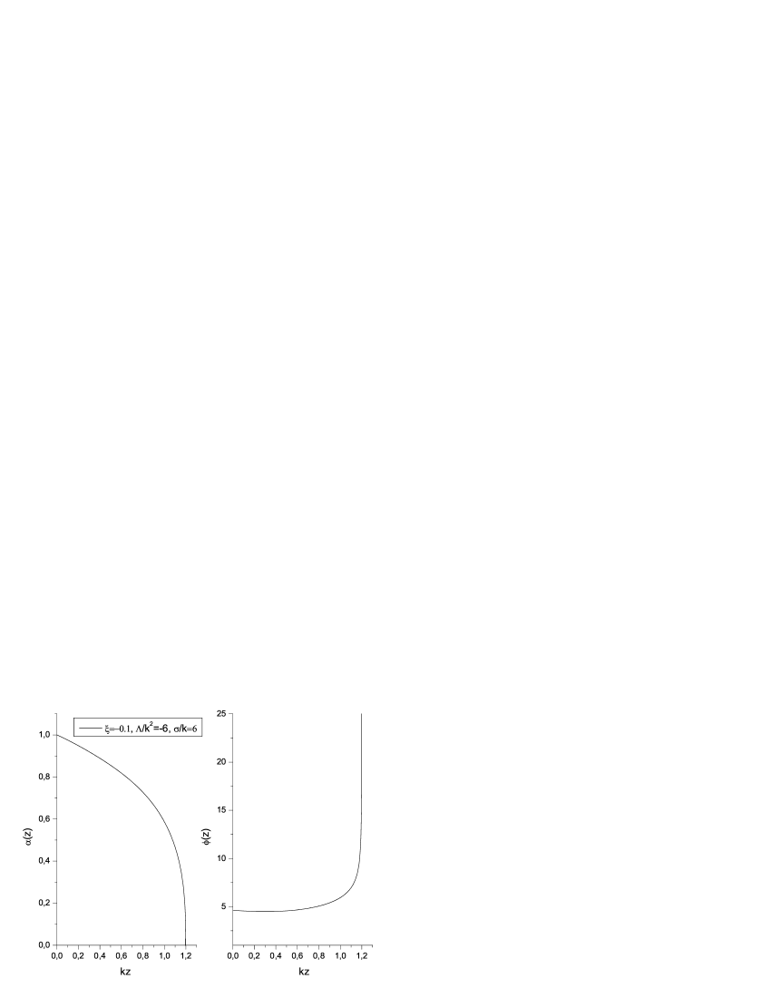
In Fig. 1 we have plotted the warp factor $a(z)$ and the scalar field $\phi(z)$ as a function of z for $\sigma/k=6$, $\Lambda/k^{2}=-6$, $\xi=-0.1$, $\lambda/k^{2}=0.01$. The values for $\sigma,\Lambda$ satisfy the fine tuning of the RS-model. We see that the metric of our model exhibits a naked singularity, as the warp factor vanishes for $kz_{s}=1.197$. Note that the warp factor for $\xi=-0.1$ is completely different from the exponential profile of the warp factor of the RS2-model.

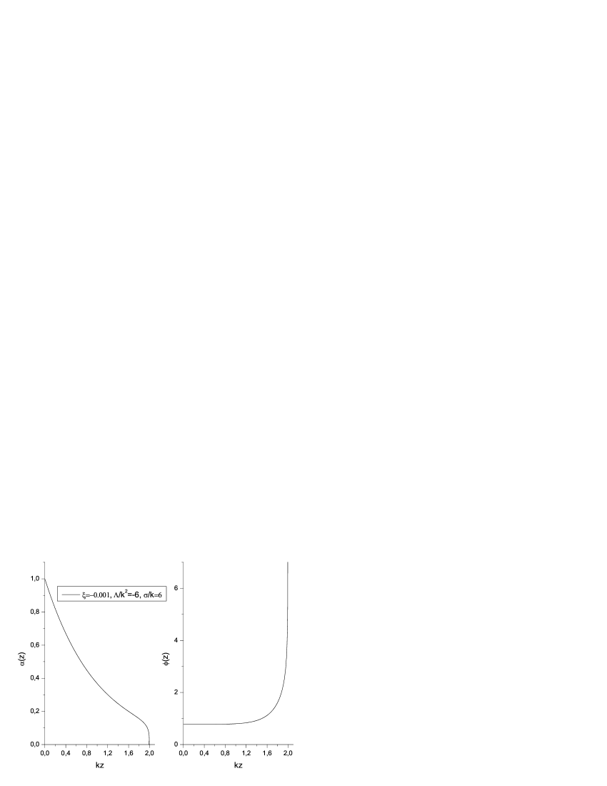
However for very small absolute values of $\xi$ (for example $\xi=-0.001$), as we see in Fig. 2, the warp factor near the brane is almost identical with the exponential profile of Eq. (2) ($a(z)=e^{-kz}$), (in Fig. 2 we we have plotted the warp factor $a(z)$ and the scalar field $\phi(z)$ as a function of z for $\sigma/k=6$, $\Lambda/k^{2}=-6$, $\xi=-0.001$, $\lambda/k^{2}=0.01$ and $k=1$). However even in this case we can not avoid a naked singularity in the bulk at $z_{s}k=1.994$. We have checked that a naked singularity in the bulk appears for arbitrarily small negative values of $\xi$.

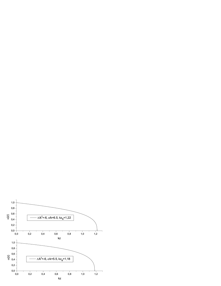
In Fig. 3 we examine the case where we have a violation of the fine tuning $\Lambda\neq-\frac{\sigma^{2}}{6}$. As a consequence, the RS2-metric of Eq. (2) (exponential warp factor) is not a solution of the RS2-model with a nonminimally coupled bulk scalar field. However, we see (Fig. 3) that this model possesses static solutions of the form of Eq. (10) with a naked singularity in the bulk. It is interesting to note that the induced metric on the brane is Minkowski, even when the fine tuning $\Lambda=-\frac{\sigma^{2}}{6}$ is violated. We remind the reader that in the case of a violation of the fine tuning, the RS2-model (without the nonminimally coupled scalar field) possesses solutions with an $AdS_{4}$ or $dS_{4}$ induced metric on the brane, see for example Ref. [14]. Of course if we wish to construct a brane world scenario, we should put a second brane in the bulk before the singularity. However, in this case the tension of the second brane $\sigma^{\prime}$, and the parameters $\Lambda$ and $\sigma$ of the first brane should be finely tuned suitably, if we want the Einstein equations and the boundary conditions on the second brane to be satisfied (see for example Ref. [2] and references therein).

Note that the numerical solutions we found for $\xi<0$ are similar to the analytic solutions in Ref. [15]. However, the model in Ref. [15] is quite different from that we assume here. In Ref. [15] it is argued that this kind of solutions may have physical interest even without a second brane. In particular, there is a possibility that quantum gravity effects near the singularity push the singularity to infinite proper distance in the bulk. In this way, the singularity acts effectively as a physical end to the extra dimension z (for more details see Ref. [15]). A way to take into account quantum gravity effects, is to add to the gravity action of Eq. (1) a Gauss-Bonnet term. We have performed numerical computations also for this case and the answer is that Gauss-Bonnet gravity can not resolve the naked singularity (see also [16]). The naked singularity remains for arbitrary values (positive or negative) of the free parameter in front of the Gauss-Bonnet term.

In our previous work [5] we pointed out the instability of both the RS2-metric of Eq. (2) and the scalar field vacuum $\phi=0$, for $\xi<0$. Responsible for this instability is the existence of a unique tachyon mode localized on the brane. By using this result in Ref [5] we tried to guess the form of the new static stable solution where the system is expected to relax. In particular, we supposed that the profile of the scalar field vacuum in the bulk is proportional to the wave function of the tachyon mode (or the scalar field vacuum is nonzero on the brane and tends rapidly to zero in the bulk). If we take for granted that $\phi(z)\rightarrow 0$ for $|z|\rightarrow+\infty$, the warp factor for $|z|\rightarrow+\infty$ must be of the form $a(z)=e^{-k|z|}$ or $a(z)=e^{k|z|}$, as only these two functions satisfy the Einstein equations if we set $\phi(z)=0$. In Ref. [5] we guess the most plausible behavior for the new static stable metric. However in this work, by solving numerically the Einstein equations with the appropriate boundary conditions, we obtain a completely different behavior for the warp factor and the scalar field vacuum. The scalar field vacuum has not the profile of the tachyon mode. As we see in Fig. 1 and Fig. 2, the warp factor vanishes in finite proper distance in the bulk, creating a naked singularity, whereas the scalar field vacuum tends to infinity as we approach the naked singularity.

Another way to try to resolve the naked singularity is to include a suitable energy momentum tensor $T_{MN}$ in the right hand side of Einstein equations (7). We have observed that an energy momentum tensor of the form $T_{zz}=c/a(z)^{4}$, with all the other components equal to zero, is possible to give stable solutions of the form we described in the previous paragraph. However, we could not find a physical explanation for an energy momentum tensor of this form.

3.2 Case (b) ($\xi>\xi_{c}$)

Figure 4: The warp factor $a(z)$, in case (b) ($\xi>\xi_{c}$), as a function of z for two values of $\sigma/k=6$ and $2$, $\Lambda/k^{2}=-6$, $\xi=\xi_{c}+1$, $\lambda/k^{2}=0.01$. Note that the solution exists even when the values of $\sigma$ and $\Lambda$ do not satisfy the fine tuning of the RS-model.

Figure 5: The $A^{\prime}(z)/k$ and $m_{eff}^{2}/k^{2}$, in case (b) ($\xi>\xi_{c}$), as a function of kz for $\sigma/k=6$, $\Lambda/k^{2}=-6$, $\xi=\xi_{c}+1$, $\lambda/k^{2}=0.01$. Note that asymptotically both the derivative $A^{\prime}(z)$ and the $m_{eff}^{2}$ tend to a constant value, or the space-time is asymptotically $AdS_{5}$.

Figure 6: The scalar field $\phi(z)$, in case (b) ($\xi>\xi_{c}$), as a function of kz for two values of $\sigma/k=6$ and $2$, $\Lambda/k^{2}=-6$, $\xi=\xi_{c}+1$, $\lambda/k^{2}=0.01$. Note that the solution exists even when the values of $\sigma$ and $\Lambda$ do not satisfy the fine tuning of the RS-model.

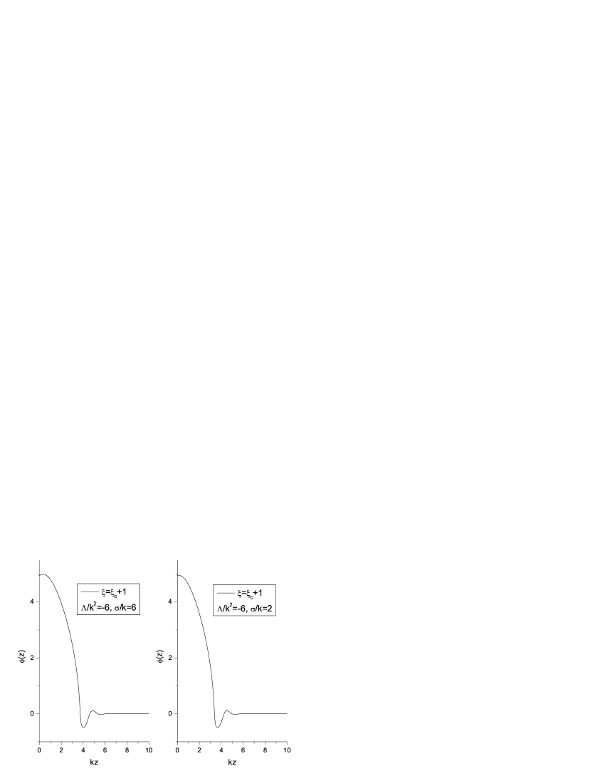
For $\xi>\xi_{c}$ we obtain a different class of numerical solutions. As we see in Fig. 4, the warp factor $a(z)$ is of the order of unity in a small region near the brane and increases exponentially ($a(z)\rightarrow e^{kz}$), as $z\rightarrow+\infty$. From this figure we can estimate that the warp factor $a(z)$ is of the order of unity for $0\leq z<3.5$ and the pure exponential behavior $a(z)=e^{kz}$ begins for $z>5$. The exponential behavior of the warp factor is confirmed with great accuracy by numerical computations, as in the left-hand panel of Fig. 5 we observe that $A^{\prime}(z)\sim 1$ for large values of z. The scalar field $\phi(z)$, as we see in Fig. 6, is nonzero on the brane (in a rather small region ($0\leq kz<4$), and for $kz>5$ tends rapidly to zero. We have checked carefully that this class of solutions appears even when $\xi$ exceeds by a small amount the conformal coupling $\xi_{c}$ ($\xi=\xi_{c}+\delta\xi$ with $\delta\xi<<1$).

Note that this class of numerical solutions is preserved even when the fine tuning $\Lambda=-\frac{\sigma^{2}}{6}$ is not satisfied (see the down panel of Fig. 4 and the right panel of Fig. 6 ($\sigma=2$, $\Lambda=-6$)). In this case also, $A^{\prime}(z)\sim 1$ for large values of z. We have checked numerically that for fixed negative $\Lambda$ there are solutions of the form of Figs. 4 and 6 only if the brane tension $\sigma$ is smaller than the absolute value of the five dimensional cosmological constant $\Lambda$.

A feature of this class of solutions is that the warp factor tends to infinity $a(z)\rightarrow e^{kz}$ for large $z$. If we wish to construct a brane world scenario, it is necessary to include a second positive tension brane far away from the first, where the numerical value of the scalar field is practically zero. In this case the tension $\sigma^{\prime}$ of the second brane should satisfy the fine tuning condition $\Lambda=\frac{-\sigma^{\prime 2}}{6}$.

However the most important topic for the construction of a realistic brane world scenario is the stability of this class of solutions. In order to study the stability, we will replace $\phi\rightarrow\phi+\hat{\phi}$ in the lagrangian

$${\cal L} = \sqrt{|g|}\left(-\frac{1}{2}g^{MN}\nabla_{M}\phi\nabla_{N}\phi-\frac{1}{2}\xi R\phi^{2}-V(\phi)\right)$$ (25)

where $\hat{\phi}$ is a small perturbation around the classic solution. If we keep only second order terms of $\hat{\phi}$, we obtain that an effective mass $m_{eff}^{2}=\xi R+12\lambda\phi(z)^{2}$ arises for the scalar field perturbation $\hat{\phi}$. In the right-hand panel of Fig. 5 we have plotted the effective mass $m_{eff}^{2}=\xi R+12\lambda\phi(z)^{2}$ as a function of z. We see that as $z\rightarrow+\infty$ the square of the effective mass tends to a constant negative value. This result indicates an instability of the solutions of class (b) against scalar field perturbation. Hence this class of solutions can not be used for the construction of realistic brane world scenarios.

3.3 Case (c) ($0<\xi<\xi_{c}$)

Figure 7: The warp factor $a(z)$ and the scalar field $\phi(z)$, in case (c) ($0<\xi<\xi_{c}$), as a function of kz for $\sigma=6$, $\Lambda=-6$, $\xi=0.1$, $\lambda=0.01$. The values for $\sigma,\Lambda$ satisfy the fine tuning of the RS-model.

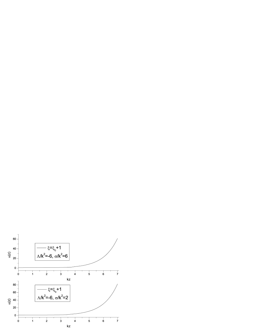
For $0<\xi<\xi_{c}$ the standard RS2-metric is stable, as there are no tachyon modes for the scalar field perturbations around this solution (see Appendix A). As we have mentioned, in this case a second static solution can be found by solving the Einstein equations numerically. This second solution exists only if Eq. (24) has at least a nonzero real root for $\phi(0)$. As we see in Fig. 7 for $0<\xi<\xi_{c}$ the warp factor $a(z)$ of this solution tends rapidly to infinity (faster than case (b)), also the scalar field $\phi(z)$ is nonzero on the brane and tends rapidly to infinity in the bulk. Contrary to case (b), where the space-time is asymptotically $AdS_{5}$, in this case the scalar curvature tends to infinity. Solutions of this kind exist even when the fine tuning of the RS-model is violated.

If we wish to construct a brane world model, we should put a second brane in the bulk. However, in order to satisfy simultaneously the three boundary conditions of Eqs. (22),(23) and (24) on the second brane, it is necessary to assume a fine tuning for the parameters of the model. Moreover, as we did in case (b), we have computed the effective mass of the scalar field around this solution and we have seen that it is positive. This implies that this class of solution is stable against perturbations of the scalar field.

4 Minimal coupling and conformal coupling

In this section we examine separately the special cases of $\xi=0$ and $\xi=\xi_{c}$. Especially in the case of conformal coupling, when the fine tuning is violated, we have a physically interesting static stable solution.

4.1 Minimal coupling $\xi=0$

The algebraic equation (24), for $\phi(0)$, can be solved analytically for $\xi=0$ or $\xi=\xi_{c}$. If we set $\xi=0$ or $\xi=\xi_{c}$ we find the equation $\lambda\phi(0)^{4}+\sigma^{2}/6+\Lambda=0$. In the case of fine tuning we obtain $\phi(0)=0$, hence the solution of the model we examine is the standard one with warp factor $a(z)=e^{-k|z|}$ and $\phi(z)=0$. If $\sigma^{2}/6+\Lambda>0$, the above equation has no real roots and our model has no static solutions. On the other hand, for $\sigma^{2}/6+\Lambda<0$ we have two real roots $\phi(0)=\pm\sqrt[4]{-\lambda^{-1}(\sigma^{2}/6+\Lambda)}$, and in this case the static numerical solutions for $\xi=0$ have the same characteristics with those of class (a) ($\xi<0$) with a naked singularity.

4.2 Conformal coupling $\xi=\xi_{c}$

Figure 8: $a(z)$, $\phi(z)$, $A^{\prime}(z)/k$ and $m_{eff}^{2}(z)/k^{2}$, for $\xi=\xi_{c}$, as a function of kz for $\sigma/k=5$, $\Lambda/k^{2}=-6$ and $\lambda/k^{2}=0.01$. Note that asymptotically both the derivative $A^{\prime}(z)$ and the $m_{eff}^{2}$ tend to a constant value, or the space-time is asymptotically $AdS_{5}$.

Figure 9: $a(z)$, $\phi(z)$, $A^{\prime}(z)/k$ and $T_{00}(z)/k^{2}$, for $\xi=\xi_{c}$, as a function of kz for $\sigma=0$, $\Lambda/k^{2}=-6$ and $\lambda/k^{2}=0.01$.

In this Section we examine the model when $\xi=\xi_{c}$ and $\Lambda\neq-\frac{\sigma^{2}}{6}$. As we have already discussed in Section 4.1, if $\sigma/k<6$, the algebraic equation (24) for $\phi(0)$ has two real roots $\phi(0)=\pm\phi_{0}$, where $\phi_{0}=\sqrt[4]{-\lambda^{-1}(\sigma^{2}/6+\Lambda)}$. In this case, the numerical solutions of the model exhibit the same characteristics with those of class (b) ($\xi>\xi_{c}$). In particular, the warp factor $a(z)$ is of the order of unity near the brane and increases exponentially ($a(z)\sim e^{k|z|}$ ), as $z\rightarrow\pm\infty$, while the scalar field $\phi(z)$ is nonzero on the brane and tends rapidly to zero in the bulk, as we can see in the upper panels of Fig. 8. The exponential behavior of the warp factor $a(z)=e^{A(z)}$ is confirmed in the down-left panel of Fig. 8. The solutions in the case of conformal coupling are of the form we described only for suitable small values of $\lambda/k^{2}$ depending on the exact value of $\sigma$ (i.e. for $\sigma=5$ we have $\lambda/k^{2}\leq 0.1$). For larger values of $\lambda$ we find a different class of solutions, however it is not of physical interest.

In the down-right panel of Fig. 8 we observe that the effective mass of the scalar field is negative. However the solutions for $\xi=\xi_{c}$ are stable, as in Appendix C we find that the scalar field does not exhibit four dimensional tachyon modes. The result of stability implies that the solutions for $\xi=\xi_{c}$ can be used as the background for the construction of a brane-world scenario.

Now we will try to discuss possible physical implications of the solutions in the case of conformal coupling. As we have already mentioned, the warp factor behaves as $e^{k|z|}$ for large $z$ (see the down-left panel of Fig. 8). It is well known that an exponentially increasing warp factor comes from negative tension brane with $-\sigma^{\prime}/k=-6$. Hence, the positive tension brane at $z=0$ $(\sigma/k=5)$ together with the negative energy density of the scalar field vacuum $T^{(\phi)}_{00}$, act effectively as a negative tension brane, which creates the exponential profile $e^{k|z|}$ for the warp factor. Note that the energy density of the scalar field has a finite size extension into the bulk of the order of $1/k$, as we see in the upper-right panel of Fig. 8. The model is completed if we include a second positive tension brane with $\sigma^{\prime}/k=6$, in a position $z_{c}$ where the scalar field vacuum is practically zero ($z_{c}>>5/k$). This two-brane set up is very similar to the well known RS1-model (see introduction). In analogy with the RS1-model, we will assume that the standard model particles live in the effectively negative tension brane, or visible brane . Note that in our case the visible brane is a formation of the positive tension brane with $\sigma/k=5$ and the negative energy density $T^{(\phi)}_{00}$ of the scalar field vacuum.

The advantage of this model is that it incorporates a mechanism for the localization of standard model particles on the visible brane. We can enrich our model with a Gauge field symmetry, i.e. SU(5) (see also [5]). We assume that this gauge field symmetry (SU(5)) is spontaneously broken to $SU_{c}(3)\times SU_{L}(2)\times U_{Y}(1)$ near the brane , due to the nonzero value of the scalar field, while it is restored in the bulk for $z>>5/k$, where the value of the scalar field is practically zero. This phase structure, Higgs phase on the brane and confinement phase in the bulk, triggers the Dvali-Shifman mechanism [6] for localization of Gauge fields. In this way the gauge fields of $SU_{c}(3)\times SU_{L}(2)\times U_{Y}(1)$ and the matter fields with gauge charge (see Ref. [2]) are localized on the brane, as for escaping in the bulk, it requires energy equal to $\Lambda_{gap}$, where $\Lambda_{gap}$ is the mass gap emerging from the nonperturbative confining dynamics of the SU(5) gauge field theory in the bulk.

In the case of the RS1-model, when ordinary matter is localized on the negative tension brane, we have the relation $M_{P}^{2}=\frac{M_{*}^{3}}{k}(e^{2kz_{c}}-1)$ (see Ref. [2]), where $M_{P}=10^{19}GeV$ is the four-dimensional Planck scale, $M_{*}$ is the fundamental five-dimensional gravity scale, k is the inverse $AdS_{5}$ radius, and $z_{c}$ is the position of the second positive tension brane in the bulk. We have checked that the above relation is valid approximately also for the model we examine. If we wish to have strong gravity at TeV we must choose $M_{*}=1TeV$. According to this localization mechanism the particles on the visible brane see an effective length toward the extra dimension of the order of $5/k$. If we take into account that the masses of ordinary particles are smaller than 1TeV, we must choose $k/5>>1TeV$. For example, if $k=100TeV$ we obtain $10M_{P}=M_{*}e^{kz_{c}}$, and thus the position of the second brane is $z_{c}\approx 39/k$.

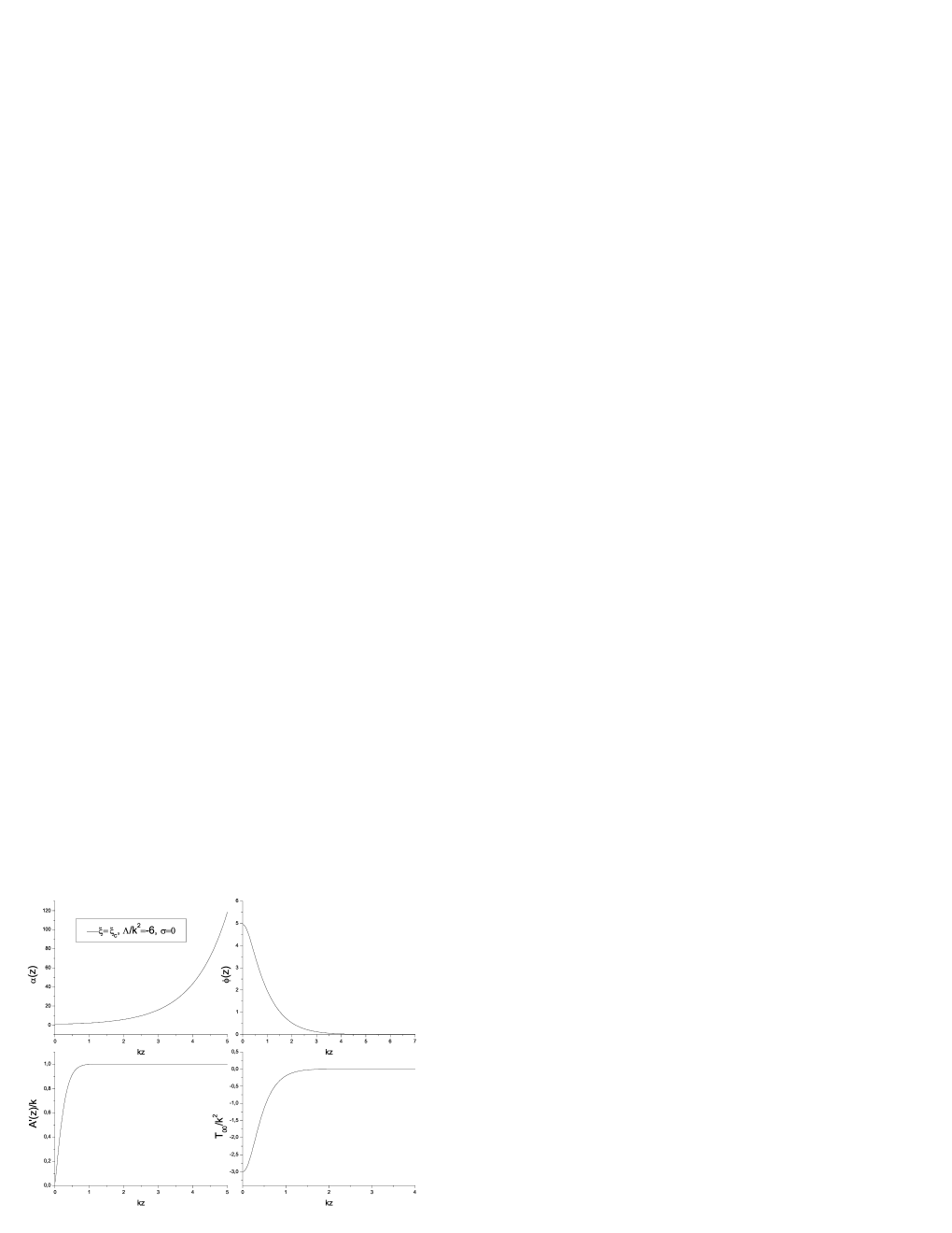
Note that even for a zero tension ($\sigma=0$) brane at $z=0$, we obtained solutions of the form we described in the previous paragraphs, see Fig. 9. In this case the visible brane is formed only from the negative energy density of the nonminimally coupled bulk scalar field, as we see in the down-left panel of Fig. 9. In addition, we have found that the numerical solutions, for small values of $\lambda/k^{2}$ ($\lambda/k^{2}\leq 0.01$), can be approximated with a very good accuracy from the analytical expressions $a(z)=\left(\cosh(\frac{|\Lambda|}{2}k|z|)\right)^{\frac{2}{|\Lambda|}}$ and $\phi(z)=\phi(0)/\left(\cosh(\frac{|\Lambda|}{2}k|z|)\right)^{\frac{1}{2}}$. These expressions satisfy the constraint equation (14). However, their second derivatives are not in agreement with the second derivatives of the numerical solutions, hence the equations (16) and (17) are not satisfied by the above mentioned analytical expressions.

5 Conclusions and discussion

In this work we studied for the first time the RS2-model with a nonminimally coupled bulk scalar field, via an interaction term ${\cal L}_{int}=-\frac{1}{2}\xi R\phi^{2}$. By solving numerically the Einstein equations with the appropriate boundary conditions on the brane, we showed that depending on the value of the nonminimal coupling $\xi$ this model possesses three classes of new static solutions with different characteristics.

Class (a) ($\xi<0$) develops a naked singularity in the bulk. Class (b) ($\xi>\xi_{c}$) consists of solutions which are characterized by an exponential warp factor $a(z)\sim e^{kz}$, as $z\rightarrow+\infty$, and a scalar field $\phi(z)$ which is nonzero on the brane and tends rapidly to zero in the bulk. The solutions of class (c) ($0<\xi<\xi_{c}$) are characterized by a very fast increase of the warp factor (faster than class (b)), and a scalar field $\phi(z)$ which tends rapidly to infinity for large $z$. The cases of minimal and conformal coupling ($\xi=0$ and $\xi=\xi_{c}$) have been discussed separately in Sections 4.1 and 4.2.

An interesting point is that these three classes of solutions exist even when the standard fine tuning of the RS-model is violated. In order to construct a brane world model by using these solutions, it is necessary to assume a second brane in the bulk. However, in this case we should impose a new fine tuning between the parameters of the model, if we wish to satisfy the boundary conditions on the second brane.

In addition, we have examined the stability properties of the new solutions. The solutions of class (a) ($\xi<0$) and class (b) ($\xi>\xi_{c}$) are unstable against scalar field perturbations, as in Appendix B we have found that the spectrum of the scalar field around these solutions exhibits a tachyon character. The only way to render these solutions stable is to put a second brane in the bulk before the potential for the scalar field V(w) becomes negative (for details see Appendix B). The solutions of class (c) are stable, as the scalar field spectrum has no tachyon modes.

We emphasize that this work has been motivated by our previous work of Ref. [5], where we had assumed the same model with an additional gauge field symmetry for the scalar field. In particular, in that work we have argued for a gravity-induced localization mechanism for $\xi<0$, which is very useful for the localization of gauge fields on the brane. In this mechanism we have a specific phase structure: confinement phase in the bulk and Higgs phase on the brane. Gauge fields, and more generally fermions and bosons with gauge charge (see Refs. [6, 2]), can not escape into the bulk unless we give them energy greater than the mass gap $\Lambda_{gap}$, which emerges from the nonperturbative confining dynamics of the gauge field model in the bulk. In Ref. [5] we observed that the effective mass $m_{eff}^{2}=\xi R$, for $\xi<0$, is negative on the brane and positive in the bulk. This result indicates a phase structure which can trigger the Dvali-Shifman mechanism in a gravitational way. We would like to emphasize that the sign of the effective mass, in the case of curved space-time, is just an indication for the expected phase structure and is not a strict proof. A realistic gravity-induced localization mechanism requires a static stable solution with a nonzero scalar field on the brane which vanishes rapidly in the bulk. In Ref. [5] we assumed the existence of a solution of the form we described above. However, the correct way to find if a solution of this kind really exists, is to solve the complete system of Einstein equations, as we do in this paper. We found that no static stable solution of the required form exists for $\xi<0$. Additionally, we obtained that for $\xi<0$ the solutions suffer from a naked singularity in the bulk, see Figs. 1,2 and 3. We tried to resolve this naked singularity by adding a Gauss-Bonnet term to the gravity action. We performed numerical computations and we found that the naked singularity remains even in the case of Gauss-Bonnet gravity. According to the above analysis, it seems that no realistic gravity-induced localization mechanism for $\xi<0$ can be constructed.

Finally, we have examined the case of conformal coupling ($\xi=\xi_{c}$) when the fine tuning of the RS-model is violated, see Section 4.1. We obtain that the solutions for $\xi=\xi_{c}$ have the same characteristics with those of the solutions of class (b) ($\xi<\xi_{c}$). However, there is an important difference between them, as the solutions for $\xi=\xi_{c}$ are stable against scalar field perturbation (see Appendix C), contrary to the case of second class, where the solutions are unstable (see Appendix B ). In Section 4.2 we argue that this class of static stable solutions can be used for the construction of a realistic brane world scenario, which is very similar to the well known RS1-model. In this scenario, the visible brane is a formation of the positive tension brane $\sigma$ at $z=0$, plus the negative energy density of the nonminimally coupled scalar field. The advantage of this model is that it incorporates a mechanism (gravity-induced Dvali-Shifman mechanism) for the localization of standard model particles on the visible brane together with the spontaneous breaking of a Grand Unified Gauge group. We would like to emphasize that the above mentioned scenario remains even in the case of a zero tension brane at $z=0$ ($\sigma=0$). In this case, the visible brane is formatted only from the negative energy density of the bulk scalar field.

6 Acknowledgements

We are grateful to Professors A. Kehagias and G. Koutsoumbas for reading and commenting on the manuscript. We also thank Professor K. Tamvakis, Professor N. Mavromatos, Dr. P. Manouselis, Dr. A. Pappazoglou and Dr. N. Prezas, for important discussions. This work was supported by the ”Pythagoras” project of the Greek Ministry of Education-European community (EPEAEK-EKT, 25/75).

Appendix A Appendix: Spectrum of scalar field perturbations around the RS2-vacuum

Figure 10: The potential $V(w)/k^{2}$ as a function of $kw$, for $\xi=-0.1$ (left-hand panel) and $\xi=\xi_{c}+1$ (right-hand panel).

Figure 11: For $\xi=\xi_{c}+1$ the spectrum of the scalar field contains exactly two tachyon modes with negative energies $m_{1}^{2}/k^{2}=-0.278$ and $m_{2}^{2}/k^{2}=-1.163$. In the figure we have plotted the wavefunctions $\psi_{1}$ and $\psi_{2}$ of the two tachyon modes as a function of $z$.

In Ref. [5] we studied the spectrum of scalar field perturbations in the background of the RS2-vacuum for $\xi<0$. In this appendix we complete this investigation by including positive values for $\xi$.

If we use the transformation

$$w=sgn(z)\frac{(e^{k|z|}-1)}{k}$$ (26)

the RS2-metric of Eq. (2) can be put into the manifestly conformal to the five-dimensional Minkowski space form

$$ds^{2}=\alpha(w)^{2}(-dx_{0}^{2}+dx_{1}^{2}+dx_{2}^{2}+dx_{3}^{2}+dw^{2})$$ (27)

where

$$\alpha(w)=\frac{1}{k|w|+1}$$ (28)

The lagrangian of the scalar field if we include an interaction term $-\frac{1}{2}R\phi^{2}$ is written as

$$L=\sqrt{|g|}\left(-\frac{1}{2}g^{MN}\nabla_{M}\phi\nabla_{N}\phi-\frac{1}{2}\xi R\ \phi^{2}-V(\phi)\right)$$ (29)

If we consider a small perturbation $\hat{\phi}$ around the scalar field vacuum ($\phi=0$) we find the corresponding linearized equation:

$$\frac{1}{\sqrt{|g|}}\;\partial_{M}\left[\sqrt{|g|}g^{MN}\partial_{N}\hat{\phi}(x,w)\right]+\xi R(w)\;\hat{\phi}(x,w)=0$$ (30)

We can set

$$\hat{\phi}(x,w)=e^{ipx}\frac{\psi(w)}{\alpha^{3/2}(w)}$$ (31)

where $\alpha(w)=1/(k|w|+1)$, and $m^{2}=p_{\mu}p^{\mu}$ is the effective four dimensional mass.

The function $\psi(w)$ satisfies the Schrondiger like equation

$$-\psi^{\prime\prime}(w)+\left[V(w)-m^{2}\right]\psi(w)=0$$ (32)

where the potential $V(w)$ is equal to

$$V(w)=\frac{(\alpha^{3/2}(w))^{\prime\prime}}{\alpha^{3/2}(w)}+\xi\alpha^{2}(w)R(w)$$ (33)

From Eqs. (27) and (32) we get

$$V(w)=-16k(\xi-\xi_{c})\left(-\delta(w)+\frac{5k}{4(k|w|+1)^{2}}\right)$$ (34)

where $\xi_{c}=3/16$ is the five dimensional conformal coupling.

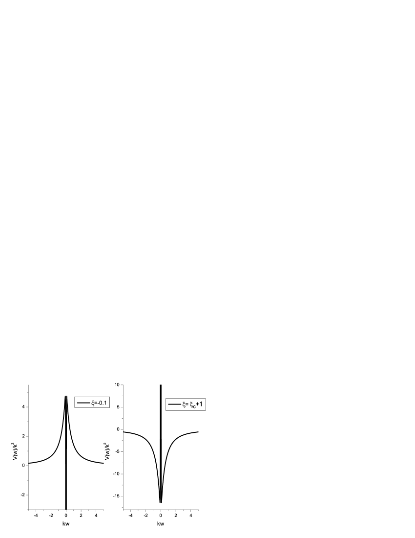
Note that the coefficient in front of the potential change sign when $\xi$ crosses the five dimensional conformal coupling. This result implies that the potential has two characteristic forms, as we see in the left-hand panel ($\xi<\xi_{c}$) and the right-hand panel ($\xi>\xi_{c}$) of Fig. 10.

In the first case, where $\xi<\xi_{c}$ the coefficient of the delta function is negative. In Ref. [5] we have shown that if $\xi<0$, the spectrum of the scalar field contains a unique tachyon mode localized on the brane (see Eq. (32) in Ref. [5]). It is well known that if $\xi=0$ there is no tachyon mode, but there is a zero mode.

For $0<\xi\leq\xi_{c}$ the potential still has the form of the left-hand panel of Fig. 10 (volcano form). However, in this case the coefficient of the delta function is not large enough in order to support a tachyon mode. We can prove this result by solving numerically the eigenvalue equation (Eq. (34) in Ref. [5]). We find that there is no tachyon mode in this region of $\xi$.

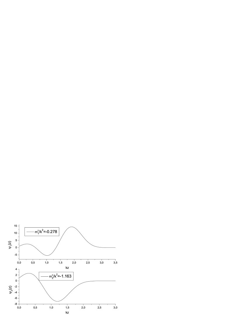
For $\xi>\xi_{c}$ the tachyon mode returns, as we obtain from Eq. (34) in Ref. [5]. However we can not use Eq. (34) (of Ref. [5]) if $\xi>1/5$, as the index of the modified Bessel functions in Eq. (34)) becomes imaginary. In this case we have solved numerically the Schrondiger equation (31) by using a shooting method and we have confirmed that indeed the spectrum of the scalar field possesses at least one tachyon mode. In particular for $\xi=\xi_{c}+1$ we have exactly two tachyon modes, and in Fig. 11 we have plotted the corresponding wave functions. Note that for $\xi>\xi_{c}$ the potential has the double-well form of the right-hand panel of Fig. 11. In this region of $\xi$ the spectrum of the scalar field is possible to contain one or more tachyon modes according to the depth of the double well.

In this appendix we studied the spectrum of scalar field perturbations around the RS2-vacuum. Depending on the value of $\xi$ we obtain that: (a) for $\xi<0$ we have unique tachyon mode, (b) for $\xi>\xi_{c}$ we have at least one tachyon mode and (c) for $0<\xi<\xi_{c}$ there are no tachyon modes. We conclude that the RS2-vacuum is unstable against scalar field perturbations in cases (a) and (b). For $\xi=0$ or $\xi=\xi_{c}$ there are no tachyon modes, hence in these cases the RS-2 vacuum is stable.

Appendix B Appendix: The tachyon character of the spectrum around the solutions of first and second class

Figure 12: The potential $V(w)/k^{2}$ as a function of $kw$, for $\xi=\xi_{c}+0.1$ in the background of second class solutions (left-hand panel) and for $\xi=-0.1$ in the background of first class solutions (right-hand panel), for $\sigma/k=6$, $\Lambda/k^{2}=-6$, ,$\lambda/k^{2}=0.01$.

In this appendix we will show that the spectrum of scalar field perturbation around the solutions of first class ($\xi<0$) and second class ($\xi>\xi_{c}$) exhibits a tachyon character. We can follow the analysis that is presented in the previous appendix. The only difference is that the value of the scalar field is nonzero in the bulk, hence the potential that appears in the Schrondiger equation (32) must be modified as

$$V(w)=\frac{(\alpha^{3/2}(w))^{\prime\prime}}{\alpha^{3/2}(w)}+\alpha^{2}(w)\left(\xi R(w)+12\lambda\phi^{2}(w)\right)$$ (35)

where $w=\int_{0}^{z}dz/a(z)$.

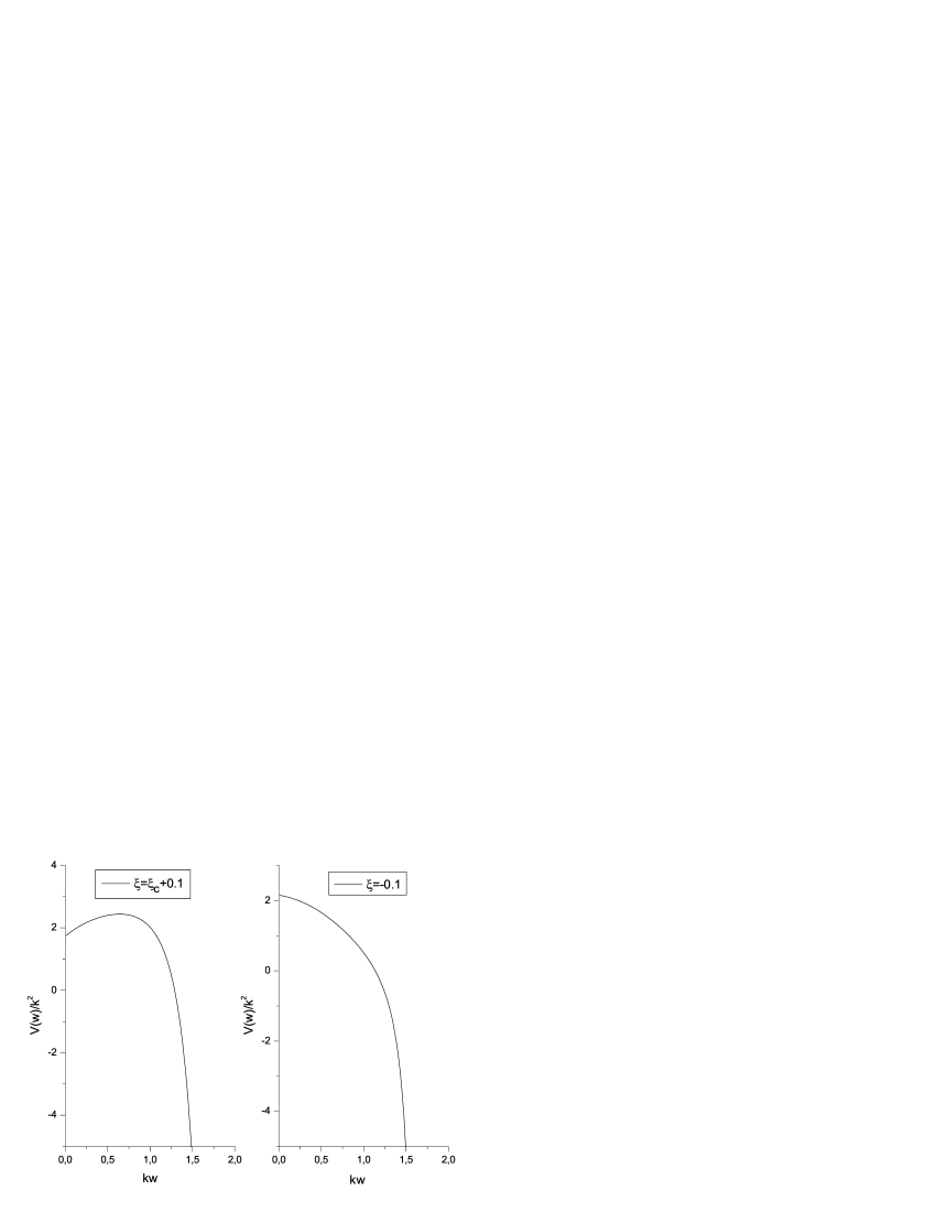
In right-hand panel and left-hand panel of Fig. 12 we have plotted the potential $V(w)$ for the first class of solutions $\xi<0$, and the second class of solutions $\xi>\xi_{c}$ respectively. As we see, the potential for both cases becomes negative and decreases without a lower bound. This implies a continuous spectrum of tachyon modes, and as a result both the first and second class of solutions are unstable. A possible way to resolve this instability is to put a second brane before the potential $V(w)$ becomes negative. In this case, a fine tuning between the parameters of the model is necessary.

Appendix C Appendix: Stable solutions for $\xi=\xi_{c}$

Figure 13: as a function of kz for $\sigma=5$, $\Lambda=-6$, $k=1$, $\lambda=0.01$.

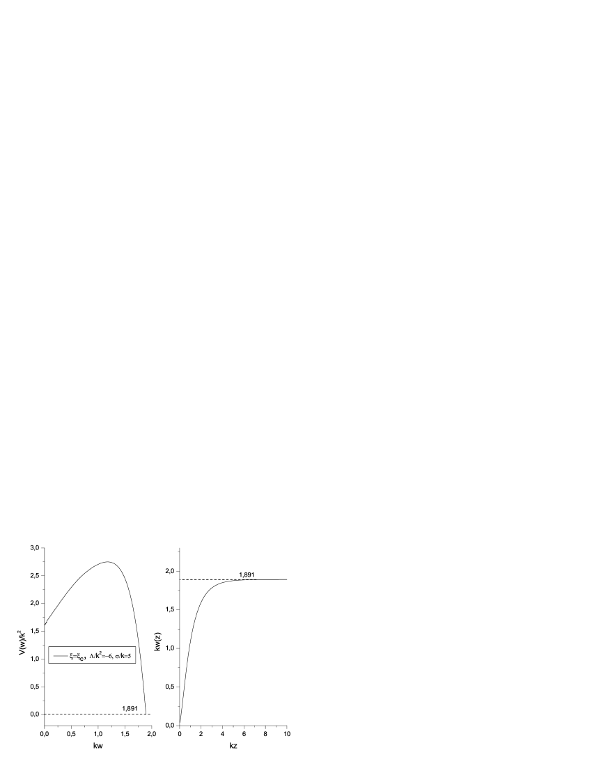
In this appendix we show that the solutions for $\xi=\xi_{c}$ are stable against scalar field perturbations. In the left-hand panel of Fig. 13 we have plotted the potential $V(w)$ (see Eq. (35)) as a function of $w$. We observe that the potential is always positive and vanishes for a finite value of the coordinate $w$ ($kw=1,891$). As we see in the left-hand panel of Fig. 13 this finite value for $w$ corresponds to infinite proper distance $z$. Thus, from the form of the potential $V(w)$ in Fig. 13 we conclude that the scalar field spectrum consists of continuous modes with positive energies, which becomes discrete in the case of a second brane in the bulk. This result implies the stability of the solutions for $\xi=\xi_{c}$.

References

- [1] N. Arkami-Hamed, S. Dimopoulos and G. Dvali, Phys. Lett. B429 (1998) 263; I. Antoniadis, N. Arkami-Hamed, S. Dimopoulos and G. Dvali, Phys. Lett. B436 (1998) 257;
- [2] V. A. Rubakov, Phys. Usp. 44 (2001) 871;
- [3] Abdel Perez-Lorenzana, An Introduction to Extra Dimensions, hep-ph/0503177.
- [4] L. Randall and R. Sundrum, Phys. Rev. Lett. 83 (1999) 3370; L. Randall and R. Sundrum, Phys. Rev. Lett. 83 (1999) 4690;
- [5] K. Farakos and P. Pasipoularides, Phys. Lett. B 621, (2005) 224-232.
- [6] G. Dvali and M. Shifman, Phys. Lett. B 396 (1997) 64.
- [7] P. Dimopoulos, K. Farakos, A. Kehagias and G. Koutsoumbas, Nucl. Phys. B 617 (2001) 237-252; P. Dimopoulos, K. Farakos, G. Koutsoumbas, Phys. Rev. D65 (2002) 074505; P. Dimopoulos, K. Farakos, Phys. Rev. D70 (2004) 045005.
- [8] M. Laine, H.B. Meyer, K. Rummukainen, M. Shaposnikov, JHEP 0404 (2004) 027.
- [9] A. Flachi and D. J. Toms, Phys Lett. B 491, (2000) 157
- [10] H. Davoudiasl, B. Lillie and T. G. Rizzo, Off-the-Wall Higgs in the Universal Randal-Sundrum Model, hep-ph/0508279; H. Davoudiasl, B. Lillie and T. G. Rizzo, Probing the Universal Randall-Sundrum Model at the ILC, hep-ph/0509160.
- [11] A. D. Dolgov, The very early universe, edited by G. W. Gibbons, S. W. Hawking and S. T. C. Siklos, (Cambrige University Press, Cambrige 1973). A. Dolgov and D. N. Pelliccia, Scalar field instabilitty in de Sitter space -time, hep-th/0502179.
- [12] L. H. Ford, Phys. Rev. D 35 (1987) 2339;
- [13] S. M. Carroll, Spacetime and geometry, Addison Wesley 2004.
- [14] A. Papazoglou, PhD Thesis, hep-ph/0112159
- [15] N. Arkani-Hamed, S. Dimopoulos, N. Kaloper and R. Sundrum, Phys. Lett. B 480 (2000) 193.
- [16] N. M. Mavromatos and J. Rizos, Phys. Rev. D62 (2000) 124004.