Gravitational waves and cosmological braneworlds:
a characteristic evolution scheme

Abstract

Motivated by the problem of the evolution of bulk gravitational waves in Randall-Sundrum cosmology, we develop a characteristic numerical scheme to solve 1+1 dimensional wave equations in the presence of a moving timelike boundary. The scheme exhibits quadratic convergence, is capable of handling arbitrary brane trajectories, and is easily extendible to non-AdS bulk geometries. We use our method to contrast two different prescriptions for the bulk fluctuation initial conditions found in the literature; namely, those of Hiramatsu et al. and Ichiki and Nakamura. We find that if the initial data surface is set far enough in the past, the late time waveform on the brane is insensitive to the choice between the two possibilities; and we present numeric and analytic evidence that this phenomenon generalizes to more generic initial data. Observationally, the main consequence of this work is to re-affirm previous claims that the stochastic gravitational wave spectrum is predominantly flat $\Omega_{\text{GW}}\propto f^{0}$, in contradiction with naive predictions from the effective 4-dimensional theory. Furthermore, this flat spectrum result is predicted to be robust against uncertainties in (or modifications of) the bulk initial data, provided that the energy scale of brane inflation is high enough.

I Introduction

It is well known that the Randall-Sundrum (RS) braneworld model Randall and Sundrum (1999a, b) is in excellent agreement with general relativity at low energies. This is the principal appeal of the model; it is one of the only examples of a scenario involving a large extra dimension that entails no serious conflicts with general relativity. However, this means that one needs to consider high energy or strong gravity scenarios to properly test the model. One possibility is to examine the high energy epoch of braneworld cosmology, where exact solutions of the 5-dimensional field equations are known. Well understood braneworld phenomena (Maartens, 2004, review) include a modified cosmic expansion and early times and ‘dark radiation’ effects, whereby the Weyl curvature of the bulk projected on the brane acts as an additional geometric source in the Friedmann equation.

But if one wants to move beyond the exact description of the background geometry in these cosmological models, there are significant technical difficulties. A cosmological brane is essentially a moving boundary in a static 5-dimensional background — anti-de Sitter space in the RS model — so perturbations are described by bulk wave equations with boundary conditions enforced on a non-trivial timelike surface. While it is possible to make some analytic progress when the brane is moving ‘slowly’ Easther et al. (2003); Battye et al. (2004); Kobayashi and Tanaka (2004); Battye and Mennim (2004), the more interesting case of a fast-moving, high-energy brane remains impervious to such treatment.

The purpose of this paper is to present a new numeric algorithm to solve wave equations in the presence of a moving boundary. For the sake of simplicity, we restrict ourselves to a class of wave equations and boundary conditions that correspond to tensor, or gravitational wave (GW), perturbations. This is not the first attempt to deal with these equations numerically: previous efforts include pseudo-spectral Hiramatsu et al. (2004, 2005); Hiramatsu (2006) and direct evolution Ichiki and Nakamura (2004a, b); Kobayashi and Tanaka (2005a, b); Kobayashi (2006) methods using various null and non-null coordinate systems in which the brane is stationary.

So why introduce another method? Our primary motivation is to develop an algorithm that offers several improvements to the preexisting efforts. Our technique is based on the highly successful characteristic integration methods from black hole perturbation theory Winicour (2005). These offer several advantages, not the least of which is an elegance of implementation that takes the causal structure of the spacetime explicitly into account. We also work in Poincaré coordinates, which greatly simplify the bulk wave equation and avoid the coordinate singularities that plague Gaussian normal patches. This makes our algorithm both transparent and unique: while other groups carry out their analysis in Poincaré coordinates, they always transform the brane to a static location for actual calculations. Our procedure is developed from first principles, and we pay careful attention to discretization errors. Hence we have a good theoretical understanding of the convergence properties of our method, which can then be tested in actual calculations. The fact that the code behaves as expected — with explicit quadratic convergence — imparts a certain level of confidence in conclusions drawn from our numerical results. Finally, our techniques should be easily adaptable to other braneworld situations; i.e., more complicated bulk geometries, sophisticated specification of initial conditions, multiple branes, etc.

Our secondary motivation stems from the fact that the numerical results found in the literature do not seem to agree with one another. In this paper, we limit the discussion to tensor type perturbations, so the principal observational consequence of our work is the present-day spectral density $\Omega_{\text{GW}}$ of relic GWs generated during inflation on the brane Maartens et al. (2000); Langlois et al. (2000); Gen and Sasaki (2001); Gorbunov et al. (2001); Kobayashi et al. (2003); Koyama et al. (2004, 2005). This ‘stochastic GW background’ is potentially observable by next-generation detectors such as the Big Bang Observatory. (Maggiore (2000) offers comprehensive review of the stochastic GW background from a 4-dimensional perspective.) Hiramatsu et al. Hiramatsu et al. (2005) (henceforth HKT) have predicted that $\Omega_{\text{GW}}\propto f^{0}$ for frequencies above some threshold $f_{c}$, whose value is determined by the curvature scale of the bulk. On the other hand, Ichiki and Nakamura Ichiki and Nakamura (2004a, b) (henceforth IN) have predicted $\Omega_{\text{GW}}\propto f^{-0.46}$ from their simulations using a different initial condition. Recently, Kobayashi and Tanaka (2005b) (henceforth KT) have applied a different numerical method to the quantum mechanical version of the problem, where one treats the entire evolution of tensor modes during inflation and radiation-domination as a particle-production phenomenon. They also derive an approximately flat spectrum for high frequencies, in agreement with HKT.

What is the right answer? It is difficult to compare these calculations directly because each group uses a different prescription for dealing with initial conditions and a different numerical method. It is sensible that when trying to solve a problem numerically, one should confirm that several independent methods yield the same results under the same circumstances. Only then can we be confident in the predictions. To this end, we attempt to reproduce the results of HKT and IN using our numerical method and their respective choices of initial conditions. We find that our numerics reproduce the HKT results within an acceptable tolerance, but we are unable to duplicate the GW spectrum predicted by IN. Indeed, we find that as long as simulations are started in sufficiently high energy epochs, both the HKT and IN initial conditions lead to the same flat spectrum.

This is an interesting and somewhat unexpected result: Superficially, the HKT, IN, and KT formulations appear quite different from one another, yet they ultimately produce the same late-time behaviour. This leads to the question: How robust is the prediction of a flat GW spectrum to arbitrary modification of the initial conditions? Answering this is the third motivation for this paper, and is a fairly ambitious goal. This is because ‘arbitrary modification’ implies the need to consider an infinite number of cases, which is highly impractical. Hence, we need to settle for qualitative conclusions drawn from numeric simulations of individual cases coupled with some approximate analytic results.

The layout of the paper is as follows: In Sec. II, we describe the problem we are going to solve in both general terms, and as specialized to tensor perturbations in RS cosmologies. The numeric algorithm used throughout the paper is developed in Sec. III, and then comprehensively tested in Sec. IV. The issue of initial conditions for GWs in braneworld cosmology is reviewed in Sec. V, and the HKT and IN approaches are explicitly contrasted in Sec. VI. A more generic class of initial data is considered in Sec. VII using a combination of numeric and analytic methods. Sec. VIII is reserved for our conclusions. Appendix A reviews the jargon associated with the stochastic GW background and how to convert the results of numeric simulations into observational predictions.

We use units in which $\hbar=c=1$ and the ‘mostly positive’ metric signature.

II Statement of the problem

II.1 Generic formulation

In this subsection, we define the generic type of problem that we solve in this paper. Consider the following wave equation:

$$[-\bm{D}^{2}+V(z)]\psi(t,z)=0.$$ (1)

Here, $D_{\alpha}$ is a covariant derivative operator on a flat 2-dimensional manifold:

$$ds^{2}=-dt^{2}+dz^{2}=-du\,dv,$$ (2)

where $u=t-z$ and $v=t+z$ are the usual retarded and advanced time coordinates. Our goal is to obtain the value of the field throughout a finite region $\Omega$ of the $(t,z)$ spacetime, which is depicted in Fig. 1.

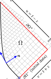
Figure 1: (Colour online.) The spacetime domain $\Omega$ over which we seek a numeric solution of the wave equation. Superimposed on $\Omega$ is a (particularly coarse) example of the computational grid we use to discretize the problem

As can be seen in this figure, the boundary of $\Omega$ is composed of three distinct parts: $\partial\Omega^{\pm}$ are null surfaces to the future and past, while $\partial\Omega_{b}$ is a timelike surface that we will refer to as the ‘brane’. The brane is defined parametrically via the equations

$$t=t_{b}(\eta),\quad z=z_{b}(\eta).$$ (3)

The parameter $\eta$ is selected to be affine in the flat $(t,z)$ geometry:

$${\bm{{u}\cdot{\partial}}}=\dot{t}_{b}\,\partial_{t}+\dot{z}_{b}\,\partial_{z},\quad{\bm{{u}\cdot{u}}}=-1.$$ (4)

Here and henceforth, we have use an overdot to denote $d/d\eta$. As long as $z_{b}\neq$ constant, the brane can said to be ‘moving’ with respect to the $(t,z)$ frame of reference. We also define a normal vector to $\partial\Omega_{b}$ pointing into $\Omega$:

$${\bm{{u}\cdot{\partial}}}=\dot{z}_{b}\,\partial_{t}+\dot{t}_{b}\,\partial_{z},\quad{\bm{{n}\cdot{n}}}=1,\quad{\bm{{u}\cdot{n}}}=0.$$ (5)

In order to have a well-defined hyperbolic problem, we must also specify initial and boundary conditions. The initial conditions consist of choosing the value of the field $\psi$ on the past null boundary $\partial\Omega^{-}$. This initial profile can be selected arbitrarily. We take the boundary conditions on the brane to be

$$0=[({\bm{{n}\cdot{D}}})\,\psi-\alpha(\eta)\psi]_{b}.$$ (6)

At this stage, we leave $\alpha$ as a finite, but otherwise arbitrary, function of ‘time’ on the brane. Therefore, this represents a wide variety of possible boundary conditions, except for pure Dirichlet $\psi(t_{b},z_{b})=0$.

II.2 Application: gravitational waves in brane cosmology

In this subsection, we show how the equations governing tensor perturbations in RS one brane cosmologies can be written in the general form introduced in Sec. II.1 above.

A cosmological RS brane is identified as a hypersurface in 5-dimension anti-deSitter space with cosmological constant $-6/\ell^{2}$:

$$ds^{2}=\frac{\ell^{2}}{z^{2}}(-dt^{2}+\delta_{ij}dx^{i}dx^{j}+dz^{2}).$$ (7)

The brane is defined by the parametric equations

$$t=t_{b}(\eta),\quad z=z_{b}(\eta),$$ (8)

such that

$$\dot{t}_{b}=\sqrt{1+\dot{z}_{b}^{2}}.$$ (9)

This equation ensures that the metric on the brane,

$$ds^{2}=a^{2}(\eta)(-d\eta^{2}+\delta_{ij}dx^{i}dx^{j}),$$ (10)

is of the standard cosmological form with $\eta$ as the conformal time, and the scale factor identified as

$$a(\eta)=\ell/z_{b}(\eta).$$ (11)

The brane’s dynamics are described by a Friedmann equation derived from the Israel junction conditions:

$$H^{2}(a)=\frac{\dot{a}^{2}}{a^{4}}=\frac{\dot{z}_{b}^{2}}{\ell^{2}}=\frac{\kappa_{4}^{2}}{3}\rho(a)\left[1+\frac{\rho(a)}{2\lambda}\right].$$ (12)

Here, $\rho$ is the density of brane matter, $\kappa_{4}^{2}=8\pi G_{4}$ is the 4-dimensional gravity-matter coupling, and $\lambda$ is the brane tension. We have enforced the RS fine tuning condition,

$$\lambda\kappa_{4}^{2}\ell^{2}=6,$$ (13)

which means that there is no net cosmological constant on the brane. We assume a single component perfect fluid for the brane matter, with equation of state $\rho=wp$, which implies $\rho\propto a^{-3(1+w)}$, as usual. This allows us to write the Friedmann equation as [$q\equiv 3(1+w)$]:

$$(H\ell)^{2}=\dot{z}_{b}^{2}=\epsilon_{*}\left(\frac{z_{b}}{z_{*}}\right)^{q}\left[2+\epsilon_{*}\left(\frac{z_{b}}{z_{*}}\right)^{q}\right].$$ (14)

Here, $\epsilon_{*}$ is the energy density of brane matter, normalized by the brane tension $\lambda$, at some reference epoch $z_{b}=z_{*}$; i.e., $\epsilon_{*}=\rho_{*}/\lambda$. Of course, $z_{*}$ is freely a specifiable length scale.

Now, we turn our attention to tensor perturbations. These are defined by the substitution

$$\delta_{ij}\rightarrow\delta_{ij}+\frac{1}{(2\pi M_{5})^{3}}\!\!\sum_{\tiny{A=+,\times}}\!\int d^{3}k\,h(t,z;\mathbf{k},A)e^{i\mathbf{k}\cdot\mathbf{x}}\varepsilon^{(A)}_{ij},$$ (15)

in the 5-dimensional metric (7). Here, $\mathbf{k}$ is a 3-dimensional wavevector, $\varepsilon^{(A)}_{ij}=\varepsilon^{(A)}_{ij}(\mathbf{\hat{k}})$ is a constant transverse trace-free polarization 3-tensor orthogonal to $\mathbf{k}$, and the summation is over polarizations. The 5-dimensional Planck mass satisfies $\ell\kappa_{4}^{2}M_{5}^{3}=1$. Unless explicitly required, we will omit the $\mathbf{k}$ and $A$ arguments from the Fourier amplitude $h$ below. One finds that $h$ obeys

$$0 = -\frac{\partial^{2}h}{\partial t^{2}}+\frac{\partial^{2}h}{\partial z^{2}}-\frac{3}{z}\frac{\partial h}{\partial z}-k^{2}h,$$ (16a)

$$0 = \left(H\ell\,\frac{\partial h}{\partial t}-\sqrt{1+H^{2}\ell^{2}}\frac{\partial h}{\partial z}\right)_{b}.$$ (16b)

Now, to put these equations into the standard form of Sec. II.1, we just need to make the definition

$$\psi(t,z)=\left(\frac{z_{*}}{z}\right)^{3/2}h(t,z).$$ (17)

Then, making use of $\dot{z}_{b}=-H\ell$ and eq. (9), we find that Eqs. (16) reduce to

$$0 = [-\bm{D}^{2}+V(z)]\psi,$$ (18a)

$$0 = [({\bm{{n}\cdot{D}}})\,\psi-\alpha(\eta)\psi]_{b}.$$ (18b)

respectively, with

$$V(z) = k^{2}+\frac{15}{4z^{2}},$$ (19a)

$$\alpha(\eta) = -\frac{3}{2}\frac{\dot{t}_{b}}{z_{b}}=-\frac{3}{2}\frac{\sqrt{1+H^{2}\ell^{2}}}{z_{b}}.$$ (19b)

Here, $n^{a}$ is defined by (5). Hence, we have successfully transformed the RS gravitational wave equation into an equivalent form defined in the flat $(t,z)$ 2-manifold. We call (18) the ‘canonical wave equation’ governing RS gravitational waves.

It is convenient to select $z_{*}$ to characterize the epoch when a perturbation with a given wavenumber $k$ enters the horizon:

$$k=a_{*}H_{*}\quad\Rightarrow\quad kz_{*}=H_{*}\ell=\sqrt{\epsilon_{*}(2+\epsilon_{*})}.$$ (20)

If we then work with the dimensionless variables

$$\hat{t}=t/z_{*},\quad\tilde{z}=z/z_{*},\quad\tilde{\eta}=\eta/z_{*},\quad\tilde{k}=kz_{*},$$ (21)

the brane equations of motion, Eqs. (9) and (14), and gravitational wave equations, Eq. (18), are completely specified by the single parameter $\epsilon_{*}$. It is useful to define a critical value $\epsilon_{c}=\sqrt{2}-1\approx 0.41$ that is associated with a perturbation that enters the horizon when $H_{*}\ell=1$. We can then classify modes as either long ($\epsilon_{*}<\epsilon_{c}$) or short ($\epsilon_{*}>\epsilon_{c}$) wavelength when compared to the characteristic length scale $\ell$ of the extra dimension. Intuitively, we expect the 5-dimensional effects to be important for short wavelength modes that enter the horizon when the universe is smaller than $\ell$.

Finally, to finishing specifying the problem, we need to fix the position of the $\partial\Omega^{\pm}$ boundaries of the computational domain in Fig. 1. This is equivalent to selecting the initial and final brane size: $z_{i}=z_{b}(\eta_{i})$ and $z_{f}=z_{b}(\eta_{f})$. It is useful to characterize the initial time by a dimensionless number $s_{0}$, which is the ratio of the perturbation’s wavelength normalized by the horizon size at the initial time:

$$s_{0}=\frac{a_{i}H_{i}}{k}=\frac{z_{*}}{z_{i}}\frac{H_{i}\ell}{H_{*}\ell}.$$ (22)

Hence, by choosing $s_{0}$ and $\epsilon_{*}$, one determines $\tilde{z}_{i}=z_{i}/z_{*}$. One can place the future boundary of $\Omega$ by selecting the ratio of the final brane size to the size at the horizon-crossing time $a_{f}/a_{*}=1/\tilde{z}_{f}$. Therefore, in dimensionless coordinates, the computational problem in Sec. II.1 is completely specified by $(\epsilon_{*},s_{0},a_{f}/a_{*})$, up to the choice of initial conditions on $\partial\Omega^{-}$. In Fig. 2, we show how the choices of $s_{0}$ and $a_{f}/a_{*}$ alter the shape of the computational domain for a radiation dominated brane ($w=1/3$).

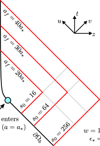
Figure 2: (Colour online.) Illustration of how the parameters $s_{0}$ and $a_{f}/a_{*}$ move the past and future null boundaries of the computational domain, respectively. Here, we have taken a radiation-dominated brane, so $\partial\Omega^{-}$ is pushed further into the past as $s_{0}$ is increased. (The opposite is true for a vacuum-dominated or deSitter brane, for example.) All other parameters being equal, the amount of CPU time required to complete one simulation scales with the area of $\Omega$ divided by the typical area of one of the cells shown in Fig. 1.

III Numeric scheme

In this section, we develop a numerical scheme for solving the class of 1+1 dimensional wave equations introduced in Sec. II.1. In subsequent sections, we will apply this scheme to the RS tensor perturbation problem described in Sec. II.2.

III.1 Computational grid

We begin by discretizing the computational domain $\Omega$ into a finite number of ‘cells’ as shown in Fig. 1. Each cell is either a diamond whose boundary consists of four null segments of equal ‘size’, or a triangle whose boundary is made up of two null and one timelike segment. The cells are arranged into rows bounded by surfaces of constant $u$ such that all diamonds in a given row have uniform size. Also, each row contains one triangle where it intersects the brane at its leftmost extreme. (In the example of Fig. 1, the triangles in the early rows are very narrow and hard to see.) The timelike segment in each triangular cell gives a straight line approximation to the brane trajectory.

Note that the diamond size generally varies from row to row. This is because we have demanded that the $u=$ constant row boundaries intersect the brane at evenly-spaced intervals of coordinate time $t$. The magnitude of this spacing is given by the parameter $\Delta$; i.e., the future boundary of the $i^{\text{th}}$ row intersects the brane at $t_{i}=t_{0}+i\Delta$, where $t_{0}$ is some initial time. Note that this is not the only possible choice; for example, we could have demanded each row be regularly spaced in $u$, $\eta$, or some other coordinate. This particular choice of spacing ensures that each diamond cell has an area less than $2\Delta^{2}$, while each triangular cell has an area less than $\Delta^{2}/4$.

III.2 Diamond cellular evolution

We now derive formulae that relate the value of the field at each node in a particular cell—these will form the heart of the integration scheme introduced in the next subsection. First, consider a typical diamond cell shown in Fig. 3(a). This type of cell has four nodes that we label by their compass directions: north, south, east, and west. The value of the field at each node is denoted by $\psi_{n}$, $\psi_{s}$, $\psi_{e}$, and $\psi_{w}$, respectively. We integrate the wave equation (1) over the cell and use Gauss’s law to obtain:

$$\int_{\partial\Diamond}({\bm{{n_{\Diamond}}\cdot{D}}})\,\psi=\int_{\Diamond}V\psi.$$ (23)

Here, $\bm{n_{\Diamond}}$ is the outward pointing normal to the cell boundary $\partial\Diamond$. In each integral, the natural ‘volume’ element on the respective submanifolds is understood. Because all of the boundary surfaces are null in a diamond cell, $\bm{n_{\Diamond}}$ is actually everywhere tangent to $\partial\Diamond$. If $\lambda$ is an affine parameter along each segment of the boundary, then we obtain

$$n_{\Diamond}^{\alpha}=\frac{dx^{\alpha}}{d\lambda}\quad\Rightarrow\quad({\bm{{n_{\Diamond}}\cdot{D}}})\,\psi=\frac{d\psi}{d\lambda}.$$ (24)

This implies that the boundary term can be evaluated exactly by integrating over the four null line segments composing $\partial\Diamond$ individually. The result is:

$$\int_{\partial\Diamond}({\bm{{n_{\Diamond}}\cdot{D}}})\,\psi=2(\psi_{e}+\psi_{w}-\psi_{n}-\psi_{s}).$$ (25)

Note that when dealing with each segment, it is important to integrate in the direction of increasing affine parameter $\lambda$, which is indicated in Fig. 3(a) by the interior arrows.

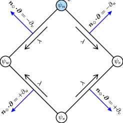
(a)   Diamond

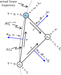
(b)   Timelike triangle

Figure 3: (Colour online.) Cellular geometries

By adopting a bilinear approximation for the integrand, the volume integral in (23) is given by

$$\int_{\Diamond}V\psi=\frac{\delta^{2}}{8}(V_{n}\psi_{n}+V_{s}\psi_{s}+V_{e}\psi_{e}+V_{w}\psi_{w})+\mathcal{O}(\delta^{4}).$$ (26)

Here, $V_{n}$ is the value of the potential at the northern node, $V_{s}$ at the southern node, and so forth; hence, $V_{n}=V_{s}$. Here, $\delta$ is the size of the cell in null coordinates. Our choice of grid spacing implies that

$$\delta\leq 2\Delta\quad\Rightarrow\quad\delta=\mathcal{O}(\Delta).$$ (27)

We now use (25) and (26) in (23) to isolate $\psi_{n}$:

$$\psi_{n}=-\psi_{s}+(\psi_{w}+\psi_{e})(1-\tfrac{1}{8}\delta^{2}V_{s})+\mathcal{O}(\Delta^{4}).$$ (28)

Given the field value at the southern, eastern and western nodes, this formula gives us the value at the northern node correct to cubic order in $\Delta$.

Note that in order to derive (28), we performed a series expansion in $V_{s}\delta^{2}$ and retained the first correction term. Hence, one should only believe the $\mathcal{O}(\Delta^{4})$ error term in the diamond evolution law when this approximation is valid; i.e., when

$$\delta^{2}V(z)\lesssim\Delta^{2}V(z)\ll 1.$$ (29)

This is sensible requirement: In order to achieve reliable results, the characteristic size of a diamond $\Delta$ must be much smaller then the characteristic length scale defined by the potential $1/\sqrt{V(z)}$.

III.3 Timelike triangle cellular evolution

We now turn our attention to the timelike triangular cells at the end of each row, an example of which is shown in Fig. 3(b). This type of cell has three nodes: north, south and east, and the boundary is composed of one timelike and two null line segments. By construction, the brane’s trajectory precisely intersects the northern and southern nodes. In the calculation that follows, we view the timelike cell boundary $\partial\triangle_{b}$ as interchangeable with the actual brane trajectory between these nodes, which we call $\partial\Omega_{b}^{(s\rightarrow n)}$. Of course, there is some degree of error associated with such an assumption, so we use a ‘$\approx$’ sign to indicate equations that are strictly true only when $\partial\Omega_{b}^{(s\rightarrow n)}=\partial\triangle_{b}$. Below, we discuss under which circumstances these ‘$\approx$’ signs can be regraded as equalities.

Integrating the wave equation over a triangular cell and applying Gauss’s law yields:

$$\int_{\partial\triangle}({\bm{{n_{\triangle}}\cdot{D}}})\,\psi=\int_{\triangle}V\psi.$$ (30)

As before, the null portions of the boundary integral can be evaluated exactly. For the timelike segment, we replace the path $\partial\triangle_{b}$ with $\partial\Omega_{b}^{(s\rightarrow n)}$. This yields

$$\int\limits_{\partial\triangle}({\bm{{n_{\triangle}}\cdot{D}}})\,\psi\approx 2\psi_{e}-\psi_{n}-\psi_{s}-\!\!\!\!\!\!\int\limits_{\partial\Omega_{b}^{(s\rightarrow n)}}\!\!\!\!\!\!({\bm{{n}\cdot{D}}})\,\psi.$$ (31)

Again, we label the field values by the node they are associated with. Using the boundary condition (6), we can substitute for the normal derivative in the brane integral. Using the trapezoid approximation, we have

$$\int\limits_{\partial\Omega_{b}^{(s\rightarrow n)}}\!\!\!\!\!\!({\bm{{n}\cdot{D}}})\,\psi=\frac{\delta_{\eta}}{2}(\alpha_{n}\psi_{n}+\alpha_{s}\psi_{s})+\mathcal{O}(\delta_{\eta}^{3}).$$ (32)

Here, $\alpha_{n}$ and $\alpha_{s}$ are the values of $\alpha(\eta)$ at the northern and southern node, respectively. The volume integral over the cell is handled via a bilinear approximation as before:

$$\int_{\triangle}V\psi=\frac{\delta_{u}\delta_{v}}{12}(V_{n}\psi_{n}+V_{s}\psi_{s}+V_{e}\psi_{e})+\mathcal{O}[(\delta_{u}^{2}+\delta_{v}^{2})^{2}].$$ (33)

Now, let us denote coordinate differences between the northern and southern nodes by $\delta_{t}$, $\delta_{z}$, etc. Our choice of grid spacing then gives

$$\delta_{t}=\Delta \Rightarrow 0\leq\delta_{\eta}^{2}\approx\delta_{t}^{2}-\delta_{z}^{2}\leq\Delta^{2}$$ (34)

$$\Rightarrow \delta_{z}\leq\Delta$$

$$\Rightarrow \delta_{u}^{2}+\delta_{v}^{2}\approx 2(\delta_{\eta}^{2}+2\delta_{z}^{2})\leq 6\Delta^{2}.$$

When we put Eqs. (30)–(34) together, we obtain

$$\psi_{n} \approx -{\frac{12+6\,\alpha_{{s}}\delta_{{\eta}}+\delta_{{u}}\delta_{{v}}V_{{s}}}{12+6\,\alpha_{{n}}\delta_{{\eta}}+\delta_{{u}}\delta_{{v}}V_{{n}}}}\psi_{s}$$ (35)

$$+{\frac{24-\delta_{{u}}\delta_{{v}}V_{{e}}}{12+6\,\alpha_{{n}}\delta_{{\eta}}+\delta_{{u}}\delta_{{v}}V_{{n}}}}\psi_{e}+\mathcal{O}(\Delta^{3}).$$

Given field values at the southern and eastern nodes, this formula gives $\psi_{n}$ accurate to quadratic order in $\Delta$, provided that the discrepancy between $\partial\Omega_{b}^{(s\rightarrow n)}$ and $\partial\triangle_{b}$ is negligible.

Under which circumstances can we ignore this discrepancy and replace the above ‘$\approx$’ signs with ‘$=$’? Clearly, when $\partial\Omega_{b}^{(s\rightarrow n)}$ is well approximated by a straight line throughout the cell. In other words, when the change $\bm{\delta u}$ in $\bm{u}$ over the cell is small. Note that because the length of $\bm{u}$ is conserved, $\bm{\delta u}$ must be parallel to $\bm{n}$, so we really want $|{\bm{{n}\cdot{\delta u}}}|\ll 1$. This condition can be rewritten as

$$|{\bm{{n}\cdot{\delta u}}}| \sim |n_{\alpha}u^{\beta}D_{\beta}u^{\alpha}|\delta_{\eta}$$ (36)

$$\lesssim |u^{\alpha}u^{\beta}D_{\beta}n_{\alpha}|\Delta$$

$$= |{\bm{{D}\cdot{n}}}|\Delta\ll 1.$$

This condition can be cast in a more geometric light by noting that in 2 dimensions, the local radius of curvature of a curve is given by $r_{c}=r_{c}(\eta)=1/|{\bm{{D}\cdot{n}}}|$. Hence, the above condition is equivalent to

$$\Delta\ll r_{c}(\eta).$$ (37)

In other words, we can reliably use the triangle evolution law (35) if the radius of curvature of the brane is much larger than the characteristic size of the cell.

III.4 The algorithm and theoretical convergence

Having defined our computational grid in Fig. 1 and derived the diamond and triangular evolution laws, (28) and (35), our algorithm for solving the wave equation (1) is quite straightforward. Referring back to Fig. 1, we see that by specifying the value of $\psi$ on $\Omega^{-}$, we gain knowledge of the field at the past boundary of row 1. An enlargement of the situation is shown in Fig. 4. To obtain $\psi$ on the future boundary of the row, we first use the triangle law to obtain the value at the node marked ‘1’ in the diagram. Then, we use the diamond evolution formula to fill in node ‘2’, then node ‘3’, and so on.

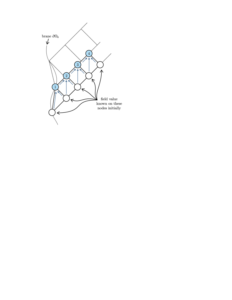
Figure 4: (Colour online.) The algorithm used to deduce the field value on the future boundary of a row, given the value on the past boundary. The numbers indicate the order in which the nodal fields are calculated, while the arrows inside the cells show how information flows through the diagram; i.e., the field value at nodes where arrows end depends directly on the field value at the nodes where the arrows start

After the field values on the future half of row 1 are found, we then need to find the field at the nodes on the past boundary of the next row. As can be seen in the diagram, those nodes do not line up with the future nodes of row 1, so we must use an interpolation scheme to determine the field there. We use a polynomial interpolation with a four-point stencil: That is, for the $i^{\text{th}}$ node on the past of row 2, we use the four closest nodes on the future of row 1 to find a cubic polynomial approximation to $\psi$. That approximation is then used to ‘fill-in’ the value of $\psi$ at the node on the past boundary of row 2. This introduces an error of order $\mathcal{O}(\Delta^{4})$ in $\psi$. Once this is accomplished for all the past nodes on row 2, we then repeat the cycle by using the evolution laws to find the field on the future of row 2, then interpolating to get $\psi$ on the past of row 3, etc.

Since we have errors of order $\Delta^{4}$ in the evolution of bulk cells and our interpolation from row to row, and errors of order $\Delta^{3}$ in cells bordering the brane, we expect our overall algorithm to exhibit quadratic convergence overall, provided that the conditions (29) and (37) are met. That is, if the ‘exact’ solution of the problem is given by $\psi_{\text{exact}}$ while our numerical solution with tolerance $\Delta$ is $\psi_{\Delta}$, we expect:

$$\psi_{\Delta}(t,z)-\psi_{\text{exact}}(t,z)=\Delta^{2}\varepsilon(t,z).$$ (38)

Here, $\varepsilon(t,z)$ is a function that does not depend on $\Delta$. We will test this convergence condition explicitly in the next section.

IV Code tests

IV.1 Inertial (de Sitter) branes

In this subsection, we specialize to RS braneworld cosmological models for which an exact solution to the tensor perturbation problem of Sec. II.2 is known. Namely, we consider de Sitter branes with $w=-1$. Our goal is to compare the results of the numerical scheme introduced in the previous subsection to this exact solution, and thus test the reliability of our algorithm.

It is convenient to introduce a new coordinate system to describe this scenario:

$$t(\eta,\xi)=\eta\cosh\xi+z_{i}\coth\xi_{b},\quad z(\eta,\xi)=-\eta\sinh\xi.$$ (39)

Here, $\xi_{b}$ and $z_{i}$ are arbitrary positive constants, the timelike coordinate $\eta$ is strictly negative, and the spacelike coordinate satisfies $\xi\geq\xi_{b}$. Then, when $w=-1$ the brane equations of motion (9) and (14) are solved by the $\xi=\xi_{b}$ hypersurface; i.e.,

$$t_{b}(\eta)=t(\eta,\xi_{b}),\quad z_{b}(\eta)=z(\eta,\xi_{b}).$$ (40)

The Hubble constant on the brane is given by $H\ell=\sinh\xi_{b}$ and we find that the brane’s speed,

$$\frac{dz_{b}}{dt_{b}}=-\tanh\xi_{b},$$ (41)

is constant; i.e., the brane trajectory in the $(t,z)$ reference frame is a straight line. One could easily call such branes ‘inertial’. Also note that when $z_{b}=z_{i}$, we have $t_{b}=0$. In Fig. 5, we show the coordinate lines of the $(\eta,\xi)$ patch in the $(t,z)$ plane. The observant reader will note that they are identical to the coordinate lines of Rindler coordinates in Minkowski space; i.e., the $\xi=$ constant lines represent a family of inertial observers whose trajectories are converging to a point and the $\eta=$ constant curves represent the surfaces over which their clocks are synchronized.

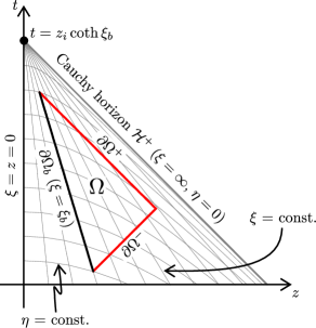
Figure 5: (Colour online.) The level curves of the Rindler-like $(\eta,\xi)$ coordinates in the $(t,z)$ plane. A brane undergoing pure-de Sitter inflation can be identified with any $\xi$ = constant surface. The solution to the tensor perturbation problem of Sec. II.2 is known exactly in these coordinates, which allows us to test the accuracy and convergence of the numeric algorithm developed in Sec. III. An example of the computational domain $\Omega$ used for the numeric calculation is also shown.

The advantage of introducing the $(\eta,\xi)$ coordinates is that they render the wave equation and boundary condition (16) separable. Hence, it is relatively straightforward to obtain an exact solution for $h=h(\eta,\xi)$. In general, this is given by a superposition of mode functions $\{\phi_{0},\phi_{\nu}\}$, with $\nu\geq 0$. The simplest of these is the so-called ‘zero-mode’,

$$\phi_{0}(\eta,\xi)=\frac{C(\sinh\xi_{b})\sinh\xi_{b}}{\ell\sqrt{2k\ell}}\left(\eta-\frac{i}{k}\right)e^{-ik\eta},$$ (42)

where

$$C(x)\equiv\left[\sqrt{1+x^{2}}+x^{2}\ln\left(\frac{x}{1+\sqrt{1+x^{2}}}\right)\right]^{-1/2}.$$ (43)

Since $h=\phi_{0}$ is a legitimate solution of (16), then

$$\psi_{\text{exact}}(t,z)=\frac{z_{*}^{3/2}}{z^{3/2}}\text{Re}\,\left\{\left[k\eta(t,z)-i\right]e^{-ik\eta(t,z)}\right\}$$ (44)

is a solution of the canonical wave equation (18), with $\eta$ defined by

$$\eta(t,z)=-\sqrt{(t-z_{i}\coth\xi_{b})^{2}-z^{2}}.$$ (45)

We also define $h_{\text{exact}}=(z/z_{*})^{3/2}\psi_{\text{exact}}$.

To test the algorithm, we proceed as follows: We set the computational domain $\Omega$ (shown in Fig. 5) by fixing a de Sitter brane trajectory, and then selecting an initial and final time. In practice, we use the dimensionless coordinates (21), so $\Omega$ and the dimensionless wavenumber $kz_{*}$ are determined by choosing $(\epsilon_{\star},s_{0},a_{f}/a_{*})$. Then, our gird is defined by the selection of a spacing $\Delta$. We synchronize our numeric solution $\psi_{\Delta}$ to the exact solution on the initial time hypersurface:

$$\psi_{\Delta}(\partial\Omega^{-})=\psi_{\text{exact}}(\partial\Omega^{-}).$$ (46)

Next, we use algorithm of Sec. III.4 to obtain $\psi_{\Delta}$ throughout $\Omega$, and then multiply by $z^{3/2}$ to get $h_{\Delta}$. We define the ‘distance’ between two arbitrary functions on the brane as

$$\langle\!\langle f_{1}-f_{2}\rangle\!\rangle_{b}=\left[\frac{1}{\eta_{f}-\eta_{i}}\int\limits_{\partial\Omega_{b}}(f_{1}-f_{2})^{2}\right]^{1/2},$$ (47)

which can be thought of as the root-mean-square (RMS) deviation between $f_{1}(\eta)$ and $f_{2}(\eta)$. Eq. (38) then predicts

$$\sigma_{b}(\Delta)\equiv\langle\!\langle h_{\Delta}-h_{\text{exact}}\rangle\!\rangle_{b}\sim\text{const.}\times\Delta^{2},$$ (48)

provided that

$$\Delta\ll r_{c}\text{ and }k\Delta\ll 1.$$ (49)

In the second inequality, we have used that $V(z)=\mathcal{O}(k^{2})$ throughout most of $\Omega$. Note that because de Sitter branes have inertial trajectories, $r_{c}=\infty$ and the first inequality is trivially satisfied.

We have calculated $\sigma_{b}$ for a wide variety of simulations of de Sitter brane scenarios and show our results in Fig. 6. Each curve represents families of simulations where $\Delta$ is varied, but all other parameters are kept fixed. We see that $\sigma_{b}$ is indeed proportional to $\Delta^{2}$ for $\Delta$ sufficiently small, which allows us to draw two conclusions: First, the numeric solution is indeed approaching the exact solution in the limit of $\Delta\rightarrow 0$; and second, the rate of convergence is quadratic. Notice that this quadratic convergence sets in for lower values of $\Delta/z_{*}$ as $\epsilon_{*}$ is increased; this is because of Eq. (20), which says that $kz_{*}$ scales like $\epsilon_{*}$ when $\epsilon_{*}$ is large. Hence, in order to satisfy $k\Delta\ll 1$, $\Delta$ must approach 0 as $\epsilon_{*}\rightarrow\infty$.

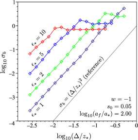
Figure 6: (Colour online.) RMS deviation between exact and numeric solutions $\log_{10}\sigma_{b}$ versus $\log_{10}(\Delta/z_{*})$ for several simulations of tensor fluctuations around inertial (de Sitter) branes. Quadratic convergence, $\sigma_{b}(\Delta)\propto\Delta^{2}$, is evidenced for $\Delta$ sufficiently small, indicating our numeric algorithm is both stable and accurate under these conditions.

IV.2 Non-inertial branes

The code tests in the last section were for manifestly non-accelerating branes, so one might reasonably worry about the reliability of our algorithm for more complicated brane trajectories. However, one cannot test the numerics in the same manner as before, precisely because no convenient exact solution to the wave equation is known for an accelerating brane. Indeed, this was one of the main motivations of developing the algorithms of Sec. III.

In the absence of an exact solution, we can test for the convergence of our numeric results, but not the accuracy. In other words, we can confirm that our results stably approach some limit (in the Cauchy sense) as $\Delta\rightarrow 0$, but we do not know if it is the right answer. A convergence test can be formulated as follows: Keeping everything else constant, we run our code once with accuracy $\sqrt{2}\Delta$ and again with accuracy $\Delta$ (the second run will take around twice as much CPU time as the first). Then, we can define the RMS discrepancy on the brane between the two runs as

$$\zeta_{b}(\Delta)=\langle\!\langle h_{\Delta}-h_{\Delta/\surd 2}\rangle\!\rangle_{b}.$$ (50)

As in the last section, eq. (38) predicts that this statistic should obey

$$\zeta_{b}(\Delta)=\text{const.}\times\Delta^{2},\quad\Delta\ll r_{c}\text{ and }k\Delta\ll 1.$$ (51)

In Fig. 7, we plot $\zeta_{b}$ versus $\Delta$ for a number of different non-inertial brane trajectories corresponding to radiation dominated brane universes. The initial condition for these simulations is simply

$$h(\partial\Omega^{-})=1.$$ (52)

Note that, to a large degree, the convergence properties of the algorithm will be independent of the initial data. We again see quadratic convergence in this figure for $\Delta$ small enough, and that smaller values of $\epsilon_{*}$ lead to faster convergence.

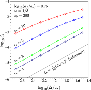
Figure 7: (Colour online.) The convergence statistic $\log_{10}\zeta_{b}$ versus $\log_{10}(\Delta/z_{*})$ for several simulations of GWs about noninertial (radiation-dominated) branes. As in Fig. 6, quadratic convergence, $\zeta_{b}(\Delta)\propto\Delta^{2}$, is apparent as $\Delta\rightarrow 0$.

From this, we can infer that our algorithm is convergent when the brane is accelerating. However, our ignorance of the exact solution means that its accuracy is still (technically) in question. The only way to get a handle on the latter is to compare our results with those independently obtained by some other group/method. This is done in Appendix VI, where we explicitly compare our results for a particular brane model to those of HKT.

V Setting the initial condition for bulk fluctuations from inflation

Having convinced ourselves that the numeric algorithm developed in Sec. III is returning reliable results, we turn attention to the physical problem we want to study. This is the the evolution of tensor perturbations in the high-energy radiation regime after the end of inflation in braneworld cosmology. In this section, we discuss the difficulties associated with determining the initial conditions of our classical problem from a quantum mechanical analysis of inflation.

The simplest picture of RS brane cosmology in the early universe assumes that the brane has some initial phase of pure-de Sitter inflation followed by a period of radiation-dominated expansion. These two distinct brane trajectories are smoothly joined at some transition point $p_{T}$ in the $(t,z)$ plane. The situation is illustrated in Fig. 8 via a conformal diagram. To generate this plot, we have applied the standard compactification to the the $(t,z)$ coordinates:

$$T=\frac{\tanh v+\tanh u}{2},\quad Z=\frac{\tanh v-\tanh u}{2}.$$ (53)

We see that the brane begins in the vicinity of past timelike infinity $i^{-}$, reaches the transition point at some finite $(t,z)$, and then continues expanding as a Friedmann brane on to future timelike infinity $i^{+}$.

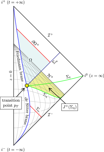
Figure 8: (Colour online.) Conformal diagram illustrating the causal structure of a braneworld model of the early universe

Now, the standard paradigm concerning braneworld GW perturbations is they are generated quantum mechanically during the de Sitter phase of the expansion. The calculation relies heavily on the $(\eta,\xi)$ Rindler-like coordinates introduced in Sec. IV.1, since the exact solution of the classical equation of motion is known exactly in that patch. The coordinate lines of this patch have been drawn on Fig. 8. One assumes that $h(\eta,\xi)$ is described by a quantum field in its vacuum state, as measured by observers travelling on $\xi=$ constant slices. We denote this ‘de Sitter invariant vacuum’ by $|0\rangle_{\eta}$. Then, one simply evaluates the vacuum expectation values of the squared amplitude of the various mode functions to see how they are magnified during inflation; for example, the zero mode amplitude is

$${}_{\eta}\langle 0|\hat{\phi}^{2}_{0}|0\rangle_{\eta}=|\phi_{0}(\eta,\xi)|^{2}=\text{function of $\eta$ only}.$$ (54)

That is, the evolution of the quantum fluctuations is determined by the amplitude of the classical mode functions, which are known exactly. In this way, Langlois et al. (2000) have shown that while the amplitude of the zero mode $\phi_{0}$ grows during inflation, the amplitudes of the so-called ‘massive modes’ $\phi_{\nu}$ are suppressed, which leads to a scale-invariant spectrum that agrees with the 4-dimensional result,

$${}_{\eta}\langle 0|\hat{h}^{2}|0\rangle_{\eta} = |\phi_{0}(\eta)|^{2}$$ (55)

$$\xrightarrow[\,0\,]{\eta} \frac{C^{2}(\sinh\xi_{b})\sinh^{2}\xi_{b}}{2k^{3}\ell^{3}}\equiv\mathcal{C}_{i}^{2}(k).$$

This quantum calculation suggests that the appropriate post-inflationary initial condition for classical GW calculations is

$$\text{inflation:}\quad h(\Sigma_{\eta})=\text{const.},$$ (56)

where $\Sigma_{\eta}$ is an $\eta=$ constant hypersurface that intersects the brane ‘at the end of inflation’ (cf. Fig. 8), which for our purposes can be taken as the transition point $p_{T}$.

But there is problem with this picture: In order to have a well-defined Cauchy problem for the fluctuations $h(t,z)$ from the transition time to the infinite future, we must have initial data on the entire $\Sigma_{u}$ hypersurface, which is the $u=$ constant line running from $p_{T}$ to $\mathcal{I}^{+}$. Now, by specifying initial data on $\Sigma_{\eta}$, we can immediately use the bulk wave equation to obtain the field value in it’s causal future $J^{+}(\Sigma_{\eta})$. But this is not sufficient to determine the value of the field on $\Sigma_{u}$; it is apparent from Fig. 8 that

$$\Sigma_{u}\nsubseteq\bar{J}^{+}(\Sigma_{\eta}).$$ (57)

Here, an overbar indicates the closure of a set. The reason that $\Sigma_{u}$ does not lie in the future domain of dependence of $\Sigma_{\eta}$ is the existence of a Cauchy horizon $\mathcal{H}^{+}$ in the $(\eta,\xi)$ coordinates. In Figs. 5 and 8, this is the future boundary of the portion of the $(t,z)$ plane covered by the de Sitter coordinates. Note that this problem is not in general mitigated by choosing to model the brane in a finite computational domain $\Omega$; as in Fig. 8, one can draw many examples where $\partial\Omega^{-}\nsubseteq\bar{J}^{+}(\Sigma_{\eta})$.

There are several ways to get around the fact that $\bar{J}^{+}(\Sigma_{\eta})$ is too small. In the literature, several authors note that the wave equation and boundary condition (16) can be solved approximately for extremely long wavelengths:

$$k\rightarrow 0,\quad h(t,z)\sim\text{constant for all $(t,z)$}.$$ (58)

The conclusion that one draws is that, in the limit, the inflation initial condition (56) is ‘consistent’ with setting $h$ = constant on some other, more suitable hypersurface. Consequently, HKT have adopted the initial conditions

$$\text{\cite[citealias]{\@@bibref{Phrase1}{Hiramatsu:2004aa}{\@@citephrase{HKT}}{}}:}\quad h(\Sigma_{t})=\text{const.},\quad h_{,t}(\Sigma_{t})=0,$$ (59)

where $\Sigma_{t}$ is the hypersurface running from the transition point $p_{T}$ to spatial infinity, as shown in Fig. 8. This is sufficient to specify the Cauchy evolution of $h$, since

$$\Sigma_{u}\subset\bar{J}^{+}(\Sigma_{t}).$$ (60)

Note that if the brane were static, this initial data would reproduce the zero mode of the original RS model:

$$\varphi_{0}(t,z)=\text{const.}\times e^{-ikt}.$$ (61)

Of course, this is not a unique prescription; IN have instead elected to enforce:

$$\text{\cite[citealias]{\@@bibref{Phrase1}{Ichiki:2004sx}{\@@citephrase{IN}}{}}: }\quad h(\Sigma_{u})=\text{const.};$$ (62)

i.e., they have set the perturbation equal to a constant on the initial null hypersurface. Both groups acknowledge that these initial condition are somewhat ad hoc; when $k=0$ they are only consistent with the inflation initial condition (56) if additional data is specified on $\mathcal{I}^{-}$, and they are not even consistent with one another for $k>0$. We will explicitly contrast the HKT and IN initial conditions in Sec. VI.

A separate approach comes from treating the quantum inflationary calculation differently. Gorbunov et al. (2001) consider a ‘junction model’ that has de Sitter and Minkowski branes attached to one another at a non-smooth transition point. They assume that the GWs are in the de Sitter invariant vacuum $|0\rangle_{\eta}$ in the infinite past, which implies quantum particle creation when the brane’s trajectory changes abruptly. At the end of the day, then derive the spectrum of GWs as seen by RS observers travelling orthogonal to $t=$ constant slices. At first glance, this would seem to be ideal since the final amplitudes are given on $\Sigma_{t}$; furthermore, the actual derived spectrum is dominated by the zero mode, and is hence consistent with the HKT initial condition (59). However, some caution is required here, since the calculation essentially involves decomposing the quantum states preferred by $z=$ constant observers in terms of those preferred by $\xi=$ constant observers. But the latter basis is only really defined to the past of the Cauchy horizon, so we may legitimately worry if the field amplitude on the entirety of $\Sigma_{t}$ is fixed in this approach. (This issue is clearly beyond the scope of the current work.)

Recently, Kobayashi and Tanaka (2005b) have modified the Gorbunov et al. calculation by smoothly joining the initial and final phases by a radiation-dominated brane. In order to calculate the Bogliobov coefficients governing particle creation, they follow the usual practice of fixing the field value in the future (on an $v$ = constant slice) and calculation what it is in the past (on an initial $v$ = constant slice like $\Sigma_{v}$ in Fig. 8). They found a subdominant amount of energy $\lesssim 10\%$ is stored in the Kaluza-Klein modes at the end of the quantum regime. Kobayashi (2006) subsequently repeated the calculations with an improved numerical scheme, which resulted in more robust predictions.

Finally, we note one additional strategy for specifying initial data; namely, to enforce boundary conditions on ${\mathcal{I}^{-}}$. Imposition such an additional constraint is enough to fix the problems associated with the inflation initial condition (56), since

$$\Sigma_{u}\subset\bar{J}^{+}(\Sigma_{\eta}\cup\mathcal{I}^{-}).$$ (63)

The real question is: what is the appropriate condition to choose? A physically sensible minimal condition would be that there is no radiative flux entering our patch of AdS space through ${\mathcal{I}^{-}}$. It would be interesting to examine this type of prescription in detail, but such a project is beyond the scope of the current work.

VI HKT versus IN formulations

In the previous section, we saw several different types of initial conditions that one could use for numerical simulations of bulk GWs in the post-inflationary epoch of brane cosmology. In this section, we explicitly compare the GWs generated by the HKT and IN initial conditions. It is useful to first identify the key qualitative features of the radiation, and to do this we concentrate on the HKT case. For simplicity, we take the HKT condition to be $h=1$ and $\partial_{t}h=0$ on an initial $t$ slice in actual calculations. Labeling the initial time as $t=0$, we can write down the exact solution of the wave equation (16) inside the causal future of $\Sigma_{t}$:

$$h(t,z)=\cos(kt)\text{ for all }(t,z)\in\bar{J}^{+}(\Sigma_{t}).$$ (64)

In particular, this can be evaluated on $\Sigma_{u}$ to give us initial data on $\partial\Omega^{-}$,

$$h(\partial\Omega^{-})=\cos\tfrac{1}{2}k(v+u_{i}),$$ (65)

where $u_{i}$ is the $u$-coordinate of the intersection of the brane with the initial time slice.

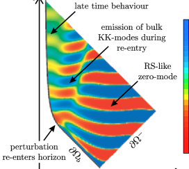
(a)   Bulk profile

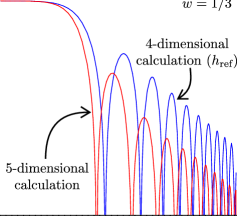
(b)   Brane profile

Figure 9: (Colour online.) Results of a typical integration using the HKT initial condition ($\Delta/z_{*}=2^{-10}\sim 10^{-3}$). In Fig. 9(b), we have drawn what the brane GW signal would be if the bulk were neglected; i.e., if one solved the 4-dimensional master equation (68) with a modified expansion rate given by (12). Note that we have enforced the initial condition that $h_{b}=h_{\text{ref}}$ for $a\ll a_{*}$ on the reference wave.

In Fig. 9, we plot the results of our numeric calculation for a particular case involving a radiation dominated brane. The key features are as follows: In the bulk, the waveform appears to retain the character of the Randall-Sundrum zero mode far away from the brane; i.e., it is constant on constant $t$ slices. However, this symmetry is broken closer to the brane by the motion of the boundary, resulting in rich and intriguing dynamics. On the brane, the GW amplitude remains constant for $a\lesssim a_{*}$, and then begins to oscillate and decay. Asymptotically, one can easily confirm that the numeric waveform goes like

$$h_{b}\xrightarrow[\,\infty\,]{a}\frac{\mathcal{C}_{b}(k)}{a}\cos\left(\omega_{0}\frac{a}{a_{*}}+\varsigma\right)=\frac{\mathcal{C}_{b}(k)}{a}\cos(k\eta+\varsigma),$$ (66)

where $\mathcal{C}_{b}(k)>0$ is the expansion-normalized characteristic amplitude, $\varsigma$ is a phase, and

$$\omega_{0}=\sqrt{1+\tfrac{1}{2}\epsilon_{*}}.$$ (67)

This asymptotic form can be understood by considering a fictional 4-dimensional universe that undergoes the same expansion (cf. Eq. 14) as our ‘real’ brane universe. Tensor fluctuations in such a model obey

$$\left(\frac{d^{2}}{d\eta^{2}}+2Ha\frac{d}{d\eta}+k^{2}\right)h_{\text{ref}}=0,$$ (68)

where the ‘ref’ subscript indicates the amplitude in our reference 4-dimensional universe. At late times, $H\ell\sim\sqrt{2\epsilon_{*}}(a_{*}/a)^{2}$ for a radiation dominated brane, leading to

$$h_{\text{ref}}(a)\xrightarrow[\,\infty\,]{a}\frac{\mathcal{C}_{\text{ref}}(k)}{a}\cos(k\eta+\varsigma_{\text{ref}}),\quad\mathcal{C}_{\text{ref}}(k)>0.$$ (69)

Hence, the late time behaviour of $h_{b}$ from the numeric simulations matches that of the 4-dimensional effective calculation. However, the amplitude of $h_{b}$ relative to $h_{\text{ref}}$ is somewhat diminished, as seen Fig. 9(b). Physically, this has to do with the brane motion inducing the radiative loss of GW energy into the bulk, as depicted by the bulk gravity wave profile seen in Fig. 9(a).

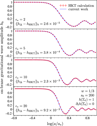
Figure 10: (Colour online.) Direct comparison of numerical results obtained by HKT and the current work ($\Delta/z_{*}=2^{-10}\sim 10^{-3}$). In each panel, the RMS deviation between the two profiles is given.

In Fig. 10, we plot our $h_{b}$ predictions for several additional cases using the HKT initial condition. For comparison, we also plot the actual numeric results obtained by HKT for the same cases. The agreement between the two independent calculations is visually excellent, with both sets of data lining up very well, but not perfectly. We can quantify the level of agreement by calculating the RMS discrepancies $\langle\!\langle h_{\Delta}-h_{\text{HKT}}\rangle\!\rangle_{b}$, which are written directly on the figures. We see that $\langle\!\langle h_{\Delta}-h_{\text{HKT}}\rangle\!\rangle_{b}\lesssim 10^{-2}$ for the cases shown, which can be interpreted as the average absolute deviation between the two results. This is acceptably small, and we can conclude that the two simulations agree to within reasonable tolerances.

Now, we turn our attention to the IN formulation. In Fig. 11, we show the radiation patterns around a $w=1$ ‘stiff matter’ brane generated by the HKT and IN initial conditions, respectively. The two bulk waveforms in Fig. 11(a) are similar to one another, but exhibit some clear differences, especially near the initial data surface $\partial\Omega^{-}$. But the the brane profiles shown in Fig. 11(b) are virtually identical to one another. Indeed, the RMS discrepancy between the two results is $\sim 10^{-4}$, which is quite small.

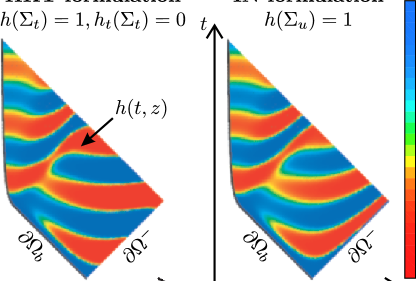
(a)   Bulk profile

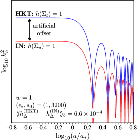
(b)   Brane profile

Figure 11: (Colour online.) GW amplitudes $h_{\Delta}(t,z)$ for a ‘stiff matter’ brane ($w=1$) using the HKT and IN initial conditions.

Is it possible that the remarkable on-brane agreement between the HKT and IN formulations is due to a serendipitous choice of parameters? In Fig. 12, we plot the discrepancy (as defined by the inner product Eq. 47) between the brane amplitude generated by the two different initial conditions as a function of the initial wavelength of the perturbation $s_{0}$. In this plot, the brane is radiation-dominated. We see the limiting behaviour

$$\langle\!\langle h_{\Delta}^{\text{(HKT)}}-h_{\Delta}^{\text{(IN)}}\rangle\!\rangle_{b}\xrightarrow[\,\infty\,]{s_{0}}0;$$ (70)

i.e., as the initial data surface $\partial\Omega^{-}$ is moved further and further into the past (cf. Fig. 2), the level of agreement between the two boundary conditions increases. This is reminiscent of a result obtained by HKT: Their on-brane waveforms showed very little dependence on $s_{0}$, provided that $s_{0}$ was large enough.

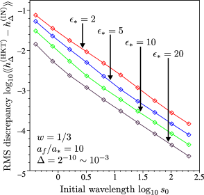
Figure 12: (Colour online.) RMS discrepancy in the $h_{b}$ waveforms generated by the HKT and IN initial conditions versus the initial wavelength $\log_{10}s_{0}$ of the perturbation.

As described in Appendix A, we need to know

$$\mathcal{R}=\frac{\mathcal{C}_{b}}{\mathcal{C}_{\text{ref}}}=\frac{\text{late time amplitude of $h_{b}$}}{\text{late time amplitude of $h_{\text{ref}}$}}$$ (71)

in order to predict the observable spectral density of GWs today. Here, we will take the post-inflationary epoch to be purely radiation-dominated. By ‘late time’, we mean that the ratio should be evaluated in the low energy regime of the cosmological evolution:

$$1\gg\frac{\rho}{\lambda}=\epsilon_{*}\left(\frac{a_{*}}{a}\right)^{4}.$$ (72)

For practical calculations, we measure the amplitude ratio when $a=20a_{*}$ and limit $\epsilon_{*}\leq 32$. In Fig. 13 we plot $\mathcal{R}$ as a function of $f/f_{c}$ for the HKT and IN initial conditions and several choices of $s_{0}$; where $f$ is the present-day frequency of the simulated wave, and $f_{c}$ is the present-day frequency of a mode that re-entered the horizon when $H\ell=1$ (cf. Eq. 112). Qualitatively, we see that for $s_{0}\lesssim 1$, there is a discernable difference in the $\mathcal{R}$ predictions from the two initial conditions. However for $s_{0}\gg 1$, the ratios are identical to one another, and satisfy

$$\mathcal{R}\propto(f/f_{c})^{-2/3},\quad f\gg f_{c}.$$ (73)

When this result is combined with (109) and (114), we find that the present day spectral density of gravitational radiation obeys

$$\Omega_{\text{GW}}\propto\left(\frac{f}{f_{c}}\right)^{0},\quad f\gg f_{c};$$ (74)

i.e., we get a flat GW spectrum in the high-frequency limit. This essentially re-confirms the main result of HKT, but with the twist that it also holds for the initial data prescription favoured by IN. However, the latter group claims the spectrum is red at high frequencies: $\Omega_{\text{GW}}\propto(f/f_{c})^{-0.46}$. The source of tension between this and the current result is unclear.

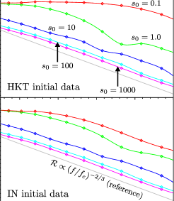
Figure 13: (Colour online.) The ratio $\mathcal{R}$ of the late-time amplitude of GWs on the brane obtained from our simulations to that of the reference wave $h_{\text{ref}}$. In all cases, we have assumed radiation domination $w=1/3$ and evaluated the ratio when $a=20a_{*}$, or equivalently $\rho/\lambda\lesssim 2\times 10^{-4}$.

VII Generic initial data

In the previous subsection we saw that if our initial data surface was set far enough into the past, the on-brane waveforms were insensitive to the choice between HKT and IN initial conditions. However, it is clear that either alternative represents a fairly restrictive choice of initial data. In this subsection, we will explore the extent to which $h_{b}$ is indifferent to more arbitrary choices of $h(\partial\Omega^{-})$. Throughout this entire section, we specialize to radiation dominated $w=1/3$ models.

VII.1 Basis functions

Generically, any initial data on $\partial\Omega^{-}$ may be decomposed as

$$h(\partial\Omega^{-})=h_{i}(v)=\frac{1}{2\pi}\int\limits_{-\infty}^{\infty}d\mu\,\mathcal{A}(\mu)e^{i\mu k(v+u_{i})/2},$$ (75)

where the Fourier amplitude $\mathcal{A}(\mu)$ is arbitrary. For example, the HKT condition is recovered if

$$\mathcal{A}(\mu)=\pi\left[\delta(\mu-1)+\delta(\mu+1)\right],$$ (76)

while the IN condition follows from

$$\mathcal{A}(\mu)=2\pi\delta(\mu).$$ (77)

Let us now define $\chi_{\mu}(\Omega)$ to be a solution of the wave equation such that $\chi_{\mu}(\partial\Omega^{-})=e^{i\mu k(v+u_{i})/2}$. Then,

$$h(\Omega)=\frac{1}{2\pi}\int\limits_{-\infty}^{\infty}d\mu\,\mathcal{A}(\mu)\chi_{\mu}(\Omega);$$ (78)

i.e., if we have knowledge of the ‘basis functions’ $\chi_{\mu}$, we can write down the solution for $h$ corresponding to arbitrary initial data. Our present goal is to numerically calculate $\chi_{\mu}$ for various situations and gain some intuition about its qualitative behaviour.

Before proceeding, it is useful to make a few remarks about $\{\chi_{\mu}\}$. First and foremost, this basis is in no way preferred or special, it is merely convenient. Its definition is intimately tied to the choice of the initial null hypersurface; hence, if $\partial\Omega^{-}$ is moved, we get a different basis. We do not expect $\{\chi_{\mu}\}$ to satisfy any type of orthogonality relationship over $\Omega$; indeed, we will not even specify what the appropriate inner product might be.

An important property of $\{\chi_{\mu}\}$ is the physical interpretation of the real and imaginary parts of the basis functions. If $\bm{p_{i}}$ is the point where the brane $\partial\Omega_{b}$ and the initial data hypersurface $\partial\Omega^{-}$ intersect, the real and imaginary parts of $\chi_{\mu}$ satisfy

$$\text{Re}\,\chi_{\mu}(\bm{p_{i}})=1,\quad\text{Im}\,\chi_{\mu}(\bm{p_{i}})=0.$$ (79)

Hence, the two independent components of any given $\chi_{\mu}$ represent distinct physical possibilities: Either the initial brane amplitude is nonzero or not. From a 4-dimensional point of view, $\text{Re}\,\chi_{\mu}$ represents a superhorizon perturbation whose non-zero amplitude is frozen until re-entry. On the other hand, $\text{Im}\,\chi_{\mu}$ is a perturbation that exists ‘entirely in the bulk’ initially; its appearance on the brane after the end of inflation would be mysterious to an observer unaware of the extra dimension. In the special case of $\mu=1$, it is easy to confirm that the imaginary part of $\chi_{\mu}$ satisfies the following initial conditions on the initial $t=$ constant surface:

$$\text{Im}\,\chi_{\mu=1}(\Sigma_{t})=0,\quad\partial_{t}\text{Im}\,\chi_{\mu=1}(\Sigma_{t})\neq 0.$$ (80)

When this is compared to (59), we see that $\text{Im}\,\chi_{\mu=1}$ satisfies a sort of ‘complimentary’ HKT condition. On the other hand, $\text{Re}\,\chi_{\mu=1}$ satisfies the HKT condition precisely.

Finally, we mention the physical interpretation of the $\mu$ parameter. If we neglect the brane boundary condition and work in the limit of $z\rightarrow\infty$, we find that

$$\chi_{\mu}\approx e^{ik(u-u_{i})/2\mu}e^{i\mu k(v+u_{i})/2}$$ (81)

is a solution of (16a) that satisfies the appropriate initial conditions on $\partial\Omega^{-}$; i.e., $u=u_{i}$. It is instructive to calculate the flux associated with this ‘solution’:

$${\bm{{j_{\mu}}\cdot{dx}}} = \frac{1}{2i}\left(\chi_{\mu}^{*}\bm{D}\chi_{\mu}-\chi_{\mu}\bm{D}\chi_{\mu}^{*}\right)\bm{\cdot dx}$$ (82)

$$\approx k(\cosh\beta\,dt+\sinh\beta\,dz),$$

where we have defined

$$\tanh\beta=\frac{\mu^{2}-1}{\mu^{2}+1}.$$ (83)

Hence, asymptotically far from the brane and the origin ($z=0$), the $\chi_{\mu}$ basis functions reduce to plane waves traveling with Lorentz boost parameter $\beta$ with respect to the static $(t,z)$ coordinates. Note that the definition of $\beta$ implies that modes with $|\mu|<1$ have wavevectors pointing towards $z=0$, while the modes with $|\mu|>1$ are traveling away from $z=0$. The HKT modes $\mu=\pm 1$ represent the middle ground: they have no relative motion with respect to the static frame. Indeed, when $\mu=\pm 1$ we have $\chi_{\mu}\approx e^{\pm ikt}$ in the asymptotic region, which are the two independent phases of the RS zero-mode.

To summarize, in this subsection we have introduced a set of basis functions in terms of which any square-integrable $h(\partial\Omega^{-})$ can be decomposed. It must be stressed that while this choice is convenient, it is arbitrary. Obviously, if we employed any other basis, the interpretation of $\mu$ would be quite different; for example, we could have selected the RS massive mode functions (evaluated on $\partial\Omega^{-}$) from the static brane case Randall and Sundrum (1999b) as a basis, which is perhaps more suited to the fact that the bulk is warped. Having said this, our choice of $\chi_{\mu}$ is extremely straightforward to implement numerically, and we feel that the $\mu$ parameter has an ‘easy’ physical interpretation: both as the relative frequency of initial data, and simply related to the Lorentz boost parameter of a plane wave irradiating the brane from $z=\infty$.

VII.2 Numerical results

In this subsection, we present our numerical results concerning the evolution of the $\chi_{\mu}$ basis functions introduced above. Note that by introducing this basis, we have increased the parameter space from $(\epsilon_{*},s_{0},a_{f}/a_{*})$ to $(\epsilon_{*},s_{0},a_{f}/a_{*},\mu)$. Each of these has a continuous spectrum, so it is very impractical to sample this parameter space densely. Instead, we will attempt to identify the principal trends in the waveform behaviour from the simulations, and go on to rationalize them with some approximate analytical work in the next subsection.

In Fig. 14, we show the bulk GW profile associated with the imaginary part of $\chi_{\mu}$ for several different choices of $\mu$. In all cases, we see that the GW profile far from the brane appears to be that of a plane wave, in agreement with the discussion of the last subsection. A white arrow indicating the expected direction of propagation of these plane waves (cf. 82) is superimposed on each plot; and we see that there is reasonable agreement between our $\chi_{\mu}$ approximation (81) and actual simulations asymptotically. Intriguingly, we see that as $\mu$ is increased, more of the initial data seems to ‘reach’ the brane. Stated in another way: When $\mu$ is small, the initial data loses its coherence when propagating from $\partial\Omega^{-}$ to $\partial\Omega_{b}$.

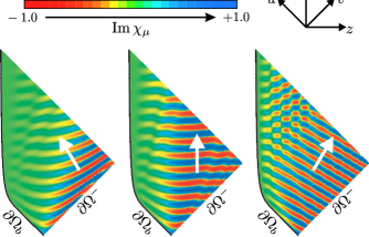
Figure 14: (Colour online.) Bulk GW profiles for $\text{Im}\,\chi_{\mu}$ initial data. Here, we have taken $(\epsilon_{*},s_{0})=(10,5)$ and $w=1/3$. The white arrows indicate the direction of the asymptotic flux derived in Eq. (82).

In Fig. 15, we plot the on-brane waveforms for cases similar to those shown in Fig. 14. Here, we see that $\text{Im}\,\chi_{\mu}$ is smaller than $\text{Re}\,\chi_{\mu}$ by several orders of magnitude, which implies that

$$\text{Re}\,\chi_{\mu}(\partial\Omega_{b})\gg\text{Im}\,\chi_{\mu}(\partial\Omega_{b})\,\,\Rightarrow\\ \chi_{\mu}(\Omega_{b})\approx\text{Re}\,\chi_{\mu}(\partial\Omega_{b}).$$ (84)

That is, at first approximation, $\chi_{\mu}(\partial\Omega_{b})$ is independent of $\text{Im}\,\chi_{\mu}$. Furthermore, the real part of $\chi_{\mu}(\partial\Omega_{b})$ shows virtually no variation as $\mu$ is increased. This leads us to hypothesize that the brane waveforms are principally determined by value of the initial data on the brane: The very weak dependence of $\chi_{\mu}(\partial\Omega_{b})$ on $\text{Im}\,\chi_{\mu}$ implies that the brane signal is insensitive to data with no initial amplitude on the brane, while the insensitivity of $\text{Re}\,\chi_{\mu}(\partial\Omega_{b})$ to $\mu$ implies that the brane signal does not overtly care about the details of initial profile in the bulk.

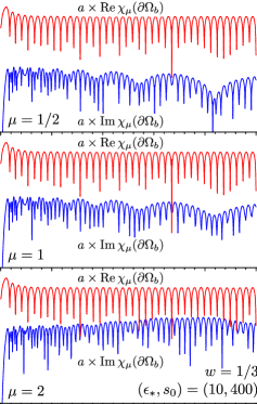
Figure 15: (Colour online.) On-brane waveforms for $\chi_{\mu}$ initial data as $\mu$ is increased and other parameters are kept constant. One can see that $\text{Re}\,\chi_{\mu}$ is relatively insensitive to $\mu$, while the opposite is true for $\text{Im}\,\chi_{\mu}$. Generally speaking, the amplitude of the imaginary part is less than the real part by several orders of magnitude.

We now want to describe how the late time amplitude of the real and imaginary parts of $\chi_{\mu}$ depend on $s_{0}$ and $\mu$. But there is small problem: It is apparent from Fig. 15 that the late time brane behaviour of $\text{Im}\,\chi_{\mu}$ is much more complicated than that of $\text{Re}\,\chi_{\mu}$. Hence, it is more difficult to obtain the asymptotic amplitude of the imaginary parts without running simulations for a very long time, which is computationally expensive. However, if we are just interested in a rough characterization of the late time amplitude, we can define the expansion-normalized average power as

$$\langle a^{2}\text{Re}^{2}\,\chi_{\mu}\rangle_{b}=\frac{1}{a_{2}-a_{1}}\int_{a_{1}}^{a_{2}}da\left[\frac{a}{a_{*}}\text{Re}\,\chi_{\mu}(\partial\Omega_{b})\right]^{2},$$ (85)

with a similar expression for $\text{Im}\,\chi_{\mu}$. For our calculations, we select the lower integration limit to correspond to an epoch well into the low-energy regime:

$$1\gg\delta=\frac{\rho_{1}}{\lambda}=\epsilon_{*}\left(\frac{a_{*}}{a_{1}}\right)^{4}.$$ (86)

On the other hand, $a_{2}$ is selected to be as large as is computationally feasible. Roughly speaking, $\sqrt{2\times\langle\text{power}\rangle}$ gives the characteristic amplitudes seen in Fig. 15.

Using the average power statistic as defined above, we study the dependence of the late time waveforms on parameters in Fig. 16. In both panels, we see that $\text{Re}\,\chi_{\mu}$ does not show much variation with either $\mu$ or $s_{0}$ for several different values of $\epsilon_{*}$. However, the imaginary parts of the basis functions change by several orders of magnitude as the parameters are varied. The principal trends are for $\langle a^{2}\text{Im}^{2}\chi_{\mu}\rangle$ to increase with $\mu$ and decrease with $s_{0}$.

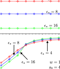
(a)   Average power as a function of initial wavelength perpendicular to the brane

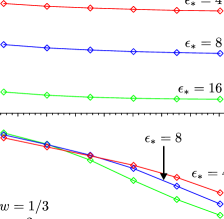
(b)   Average power as a function of initial wavelength parallel to the brane

Figure 16: (Colour online.) Expansion-normalized average power of the real and imaginary parts of $\chi_{\mu}$ as functions of parameters. To calculate the average, we have selected $\delta=10^{-3}$ and $a_{2}=50a_{*}$. The average power at late times is not very sensitive to these choices.

The physical inferences we can draw from the numeric work of this subsections is as follows: The late time behavior of perturbations on the brane is largely fixed by the value of initial data at the brane for a large range of parameters and choices of $h_{i}(v)$. The degree to which $h_{b}$ is oblivious to the bulk initial data profile increases as the initial data surface is pushed further and further into the past (cf. Fig. 2). Conversely, we find that these conclusions are mitigated if the Fourier spectrum of the initial data along $\partial\Omega^{-}$ involves high frequencies. In such cases, the bulk initial data finds it ‘easier’ to reach the brane directly.

The main observational inference of our simulations is that, for $\mu$ less than some cutoff $\mu_{c}$, the late time behaviour of the basis functions independent of $\mu$ and given by

$$\chi_{\mu}(\partial\Omega_{b})\xrightarrow[\infty]{\eta}\frac{\mathcal{C}_{b}}{a}\cos(k\eta+\varsigma),\quad\text{for all }\mu\lesssim\mu_{c}.$$ (87)

In general $\mu_{c}$ will be a function of $s_{0}$, and we expect that $\mu_{c}\rightarrow\infty$ for $s_{0}\rightarrow\infty$. The exact definition of $\mu_{c}$ will depend on how rigorously one wants to enforce the approximate asymptotic form (87). Now, if the amplitude components of a particular initial data profile satisfy

$$\mathcal{A}(\mu)\approx 0\text{ for }\mu\gtrsim\mu_{c},$$ (88)

the late time waveform follows directly from (78):

$$h_{b}\xrightarrow[\infty]{\eta}h_{i}(v_{i})\times\frac{\mathcal{C}_{b}}{a}\cos(k\eta+\varsigma),$$ (89)

where $h_{i}(v_{i})$ is just the initial data at the brane position. By definition, the reference wave introduced in Sec. VI is also linear in $h_{i}(v_{i})$, so the 5D/4D amplitude ratio $\mathcal{R}$ — and hence $\Omega_{\text{GW}}$ — will be independent of the details of the initial data profile, provided that the condition (88) is met. In other words, for finite $s_{0}$ we expect the late time gravitational wave spectrum to be independent of the detailed shape of the initial data profile, provided that that profile does not involve high frequency features. From this, it follows that the prediction of a flat GW spectrum derived from the HKT and IN formulations will generalize to more generic initial data.

VII.3 Analytic results

The inferences of the last subsection are just that: informed intuition about the behaviour of initial data based on the experience gleaned from a finite number of simulations. We can put them on somewhat surer footing by doing some approximate analytic calculations, which is the purpose of this subsection.

Let us analyze the behaviour of the wavefunction $\psi$ in the high-energy epoch of the cosmological evolution. To be more precise, we limit our attention to modes with $\epsilon_{*}\gg\epsilon_{c}\approx 0.41$; i.e., modes that have $H_{*}\ell\gg 1$. This implies that the slope of the bulk brane trajectory when $a=a_{*}$ is

$$\left(\frac{dz_{b}}{dt_{b}}\right)_{a=a_{*}}=-\frac{H_{*}\ell}{\sqrt{1+(H_{*}\ell)^{2}}}\approx-1.$$ (90)

Hence, the brane trajectory is very nearly null for $a\lesssim a_{*}$; here, we will boldly assume that it is exactly null. The computational domain $\Omega$ for this situation is illustrated in Fig. 17. We label the brane’s position at horizon re-entry as $\bm{p_{*}}=(u_{*},v_{*})$, and define $\Pi$ to be the portion of $\Omega$ located to the past of $u=u_{*}$. Our goal is to approximate the field on the future boundary $\partial\Pi^{+}$ of $\Pi$ given initial data on $\partial\Omega^{-}$.

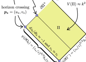
Figure 17: (Colour online.) Spacetime geometry used to rationalize the behaviour seen in the numeric simulations of Sec. VII.2 using an approximate retarded Green’s function.

Note that since we are assuming that $\epsilon_{*}$ is large, then $kz_{*}=\sqrt{\epsilon_{*}(2+\epsilon_{*})}$ is also large; i.e., $k\gg 1/z_{*}$. This means that the potential in the bulk wave equation (18) satisfies

$$V(z)=k^{2}+\frac{15}{4z^{2}}\approx k^{2},\quad\text{for }z\geq z_{*}.$$ (91)

With this, we can immediately write down an approximate retarded Green’s function for the bulk wave equation with $(\bm{p},\bm{p^{\prime}})\in\Pi$:

$$G(\bm{p};\bm{p^{\prime}})=\frac{1}{2}J_{0}(k\lambda)\theta(u-u^{\prime})\theta(v-v^{\prime}),\\ (-\bm{D}^{2}+k^{2})\,G(\bm{p};\bm{p^{\prime}})=\delta(\bm{p}-\bm{p^{\prime}}).$$ (92)

Here, we have defined $\lambda=\sqrt{(u-u^{\prime})(v-v^{\prime})}$ which is the proper time interval between the source point $\bm{p^{\prime}}$ and the field point $\bm{p}$. In terms of this Green’s function, we can express the value of $\psi$ at any $\bm{p}\in\Pi$ as:

$$\psi(\bm{p})\approx\int\limits_{\partial\Pi}\bm{n\cdot}\left[G(\bm{p};\bm{p^{\prime}})\bm{D^{\prime}}\psi(\bm{p^{\prime}})-\psi(\bm{p^{\prime}})\bm{D^{\prime}}G(\bm{p};\bm{p^{\prime}})\right].$$ (93)

Here, the integration is over $\bm{p^{\prime}}$, $\bm{n}$ is the outward pointing normal, and $\bm{D^{\prime}}$ indicates the derivative with respect to $\bm{p^{\prime}}$; i.e., differentiation with respect to the primed coordinates. The approximation sign comes from the fact that $G$ is not the ‘true’ Green’s function.

Let us now push $\bm{p}$ to the future boundary $\partial\Pi^{+}$ of $\Pi$. Since the Green’s function has support when $\bm{p}$ is in the future of $\bm{p^{\prime}}$, to calculate the integral (93) we need only specify the field values on $\partial\Omega^{-}$ and the portion of the brane $\partial\Omega_{b}$ to the past of $\partial\Pi^{+}$. We leave the initial data on $\partial\Omega^{-}$ arbitrary:

$$\psi(\partial\Omega^{-})=\left(\frac{z_{*}}{z}\right)^{3/2}h_{i}(v).$$ (94)

However when the brane trajectory is null, the boundary condition (16b) reduces to

$$\left(\frac{\partial h}{\partial u}\right)_{b}\approx 0\,\,\Rightarrow\,\,\psi(\partial\Omega_{b})\approx\left(\frac{z_{*}}{z}\right)^{3/2}h_{i}(v_{i});$$ (95)

i.e., $h$ is constant on the brane before horizon crossing, which is entirely consistent with our numeric simulations. Using this boundary data, simplifying the integral (93) is straightforward, but tedious. The result is:

$$\psi(\bm{p})\approx(2z_{*})^{3/2}\Bigg{[}3h_{i}(v_{i})\int\limits_{u_{i}}^{u_{*}}du^{\prime}\frac{J_{0}(k\lambda_{1})}{(v_{*}-u^{\prime})^{5/2}}+\\ \int\limits_{v_{i}}^{v_{p}}dv^{\prime}J_{0}(k\lambda_{2})\underbrace{\frac{\partial}{\partial v^{\prime}}\frac{h_{i}(v^{\prime})}{(v^{\prime}-u_{i})^{3/2}}}_{\mathcal{O}(h_{i}^{\prime}/u_{i}^{3/2})}-J_{0}(k\lambda_{3})\underbrace{\frac{h_{i}(v_{i})}{(v_{i}-u_{i})^{3/2}}}_{\mathcal{O}(h_{i}/u_{i}^{3/2})}\Bigg{]},$$ (96)

where we have defined

$$\lambda_{1}=\sqrt{(u_{*}-u)(v_{p}-v_{*})},$$

$$\lambda_{2}=\sqrt{(u_{*}-u_{i})(v_{p}-v)},$$

$$\lambda_{3}=\sqrt{(u_{*}-u_{i})(v_{p}-v_{i})}.$$ (97)

To arrive at this expression, we have used integration by parts to remove derivatives of the Green’s function.

The approximation (96) can be used to justify the trends we have seen above, if we note that both the initial data hypersurface and horizon crossing epoch are in the high-energy regime:

$$s_{0}=\frac{H_{i}a_{i}}{H_{*}a_{*}}\approx\sqrt{\frac{\epsilon_{*}}{2+\epsilon_{*}}}\left(\frac{v_{i}-u_{i}}{v_{*}-u_{*}}\right)^{3}\xrightarrow[-\infty]{u_{i}}\mathcal{O}(-u_{i}^{3}).$$ (98)

When inserted in (96), this yields

$$\psi(\bm{p})\approx(2z_{*})^{3/2}3h_{i}(v_{i})\int\limits_{u_{i}}^{u_{*}}du^{\prime}\frac{J_{0}(k\lambda_{1})}{(v_{*}-u^{\prime})^{5/2}}\\ +\int dv\,\mathcal{O}(h_{i}^{\prime}s_{0}^{1/2})+\mathcal{O}(h_{i}s_{0}^{1/2}).$$ (99)

If we then hold the initial $h_{i}(v)$ profile constant, as in Fig. 16(b), we see that the last two terms drop out as $s_{0}\rightarrow\infty$. Hence, we have shown that as the initial data surface goes to the infinite past, the wavefunction on $\partial\Pi^{+}$ depends only on the value of the initial data on the brane $h_{i}(v_{i})$ — and not on the initial data in the bulk $h_{i}(v>v_{i})$. Since the evolution of the GWs to the future of $\partial\Pi^{+}$ depends only on the field value on $\partial\Pi^{+}$, we can conclude that the entire late time brane waveform is determined by $h_{i}(v_{i})$ in the limit $s_{0}\rightarrow\infty$. This explains the behaviour seen in Fig. 16(b).

Now, consider the situation if we hold the position of the initial data hypersurface constant and vary the initial data profile, as in Fig. 16(a). Let us also assume that $s_{0}$ is large and that $h_{i}(v)=\mathcal{O}(1)$. Then, the third term on the righthand side of (99) is not important relative to the first. However, the second term can be arbitrarily large if we allow for initial data with large gradients $h^{\prime}_{i}(v)$. In particular if we have $h_{i}(v)=e^{i\mu k(v+u_{i})/2}$, which is the initial data that generates $\chi_{\mu}$, we see that the second term grows with $\mu$. Hence, we have shown that if the initial data on $\partial\Omega^{-}$ involves a significant high frequency component, then the late time brane waveform will be sensitive to the precise form of $h_{i}(v)$. This rationalizes the behaviour seen in Fig. 16(a).

VIII Conclusions

In this paper, we have developed a new numeric algorithm (from first principles) to deal with the problem of solving $(1+1)$-dimensional wave equations in the presence of a moving boundary. Our technique, which is based on characteristic integration methods from black hole perturbation theory, has demonstrated itself to be both reliable and accurate by reproducing previously known analytic and numeric results; and it is the principle result of this work.

We have applied our formalism to the cosmological problem of the evolution of GWs in the Randall-Sundrum one-brane scenario. One can find at least three different prescriptions in the literature Ichiki and Nakamura (2004b); Kobayashi and Tanaka (2005b); Hiramatsu et al. (2005) for how to specify post-inflationary bulk initial conditions in such models, which yield at least two contradictory predictions for the spectral tilt of the stochastic GW background generated by brane inflation. Until now, it was unclear if the discrepancy between various results was due to different choices of initial data or the numeric scheme used to evolve GWs through the high-energy radiation era after inflation. Using our code, we have investigated the initial conditions proposed by HKT and IN, and we find no discrepancy between the late time GW spectrum generated by either prescription, provided that the initial data hypersurface is set far enough into the past. Observationally, this means that both initial conditions lead to a flat GW spectrum $\Omega_{\text{GW}}\propto(f/f_{c})^{0}$ at frequencies higher that a threshold $f_{c}$ set by the curvature scale of the bulk. This is also in agreement with the results of KT, who study the quantum (i.e. not classical) evolution of the GW wavefunction.

We have also considered more general initial data by introducing a practical basis in which to decompose general solutions of the wave equation. Numerically, we find that the late time brane waveform is not very sensitive to the detailed initial data profile if we start our simulations at sufficiently high energies. However, this approximation breaks down if the Fourier transform of the initial data involves very high frequencies. We have used an approximate Green’s function analysis to analytically rationalize these results and demonstrate how they apply to any initial data; not just the choices we modelled explicitly.

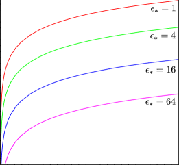
Figure 18: (Colour online.) Wavelength of perturbations at the end of inflation as a function of the inflationary energy scale.

So, is the high-frequency stochastic GW spectrum predicted from this class of braneworld models really flat? The answer seems to depend rather intimately on the energy scale of inflation. Throughout this paper, we have treated $s_{0}$ as a free parameter, and our results on the insensitivity to initial data depend on the limit $s_{0}\rightarrow\infty$. But really, we should fix the energy scale of inflation $E_{\text{inf}}\equiv H_{\text{inf}}\ell$ and synchronize $\partial\Omega^{-}$ with the beginning of the high-energy radiation era. This means that $s_{0}$ is actually a function of $\epsilon_{*}$ and $E_{\text{inf}}$:

$$s_{0}(\epsilon_{*},E_{\text{inf}})=\frac{E_{\text{inf}}^{3/4}}{\sqrt{\epsilon_{*}(2+\epsilon_{*})^{2}}}\left[\frac{E_{\text{inf}}}{\sqrt{1+E_{\text{inf}}^{2}}-1}\right]^{1/4}.$$ (100)

For reference, we have plotted $s_{0}$ as a function of $E_{\text{inf}}$ in Fig. 18. As can be seen from this plot, if we consider moderate inflationary energy scales $E_{\text{inf}}\lesssim 10^{3}$, it is possible to have $s_{0}\lesssim 10^{2}$ for reasonable values of $\epsilon_{*}$. The results of Sec. VII imply that such values of $s_{0}$ imply the dependence of the late time waveforms on initial data is weak, but non-trivial. This suggests to us that the greatest chance of obtaining deviations from the flat spectrum lies in models with small inflationary energy scales. In such scenarios, it is possible for the brane signal to carry a signature of $h(\partial\Omega^{-})$, which in turn depends on the details of the inflationary model. On the other hand, if the inflationary energy scale is high, the brane signal will only depend on the value of the perturbation on the brane at the end of inflation. Investigating the detailed gravitational wave spectrum generated by moderately low-energy brane inflation is an interesting avenue for future work.

Appendix A Characterizing the gravity wave background

In this appendix, we review how to map the results of our calculations into observable predictions concerning the spectrum of the cosmological GW background today. The treatment is very much the same as in Refs. Hiramatsu et al. (2005); Ichiki and Nakamura (2004b).

On the brane, the complete GW perturbation is written as

$$h_{ij}(\tau,\mathbf{x})=\frac{a^{2}}{(2\pi M_{5})^{3}}\sum_{A=+,\times}\int d^{3}k\,h_{b}(\tau;\mathbf{k},A)e^{i\mathbf{k}\cdot\mathbf{x}}\varepsilon^{(A)}_{ij}(\mathbf{\hat{k}}),$$ (101)

Here, $\tau$ is the cosmic time; i.e., $ds^{2}=-d\tau^{2}+a^{2}d\mathbf{x}^{2}$ on the brane. The energy density associated with this perturbation is

$$\rho_{\text{GW}}=\frac{1}{4\kappa_{4}^{2}}\bigg{\langle}\frac{dh^{*}_{ij}}{d\tau}\frac{dh^{ij}}{d\tau}\bigg{\rangle},$$ (102)

where the angular brackets indicate an average over some region of spacetime. To preform the spatial average, we make the standard assumption that the background is unpolarized, stationary, and isotropic. This means we can trade the operation of spatial averaging over $\mathbf{x}$ for ensemble averaging at $\mathbf{x}=0$, and the Fourier amplitudes obey:

$$\langle h_{b}(\tau;\mathbf{k},A)h_{b}^{*}(\tau;\mathbf{k}^{\prime},A^{\prime})\rangle=\\ (2\pi M_{5})^{3}\delta_{AA^{\prime}}\delta(\mathbf{k}-\mathbf{k}^{\prime})|h_{b}(\tau;\mathbf{k},A)|^{2}.$$ (103)

The product of polarization tensors can then be reduced via

$$\varepsilon^{(A)}_{ij}(\mathbf{\hat{k}})\,\varepsilon^{(A)ij}(\mathbf{\hat{k}})=2.$$ (104)

Temporal averaging in the late universe can be done by noting that in the late universe, our numeric results give that $h_{b}$ is a superposition of the $e^{\pm ik\eta}/a$ ‘zero-mode’ functions. Neglecting scale factor derivatives and using $\eta\approx\tau/a$ yields

$$\bigg{\langle}\left|\frac{dh_{b}(\tau;\mathbf{k},A)}{d\tau}\right|^{2}\bigg{\rangle}_{\tau}=\frac{k^{2}\mathcal{C}_{b}^{2}(k)}{2a^{4}},$$ (105)

where $\mathcal{C}_{b}(k)$ is the expansion-normalized characteristic amplitude (cf. Eq. 69). To relate $\mathcal{C}_{b}(k)$ to the primordial GW spectrum, we make use of the reference wave $h_{\text{ref}}$ discussed in Sec. VI. Our numeric simulations can be used to find

$$\mathcal{R}=\frac{\mathcal{C}_{b}}{\mathcal{C}_{\text{ref}}};$$ (106)

i.e., the ratio of the characteristic amplitudes in the low-energy regime. This is useful because the evolution of the reference wave through the high-energy radiation epoch is extremely simple: Essentially, it remains constant until $a=a_{*}$, then its amplitude decays as $1/a$. Hence, we can write

$$\mathcal{C}^{2}_{\text{ref}}(k)\approx a^{2}_{*}\mathcal{C}^{2}_{i}(k)=(k/H_{*})^{2}\mathcal{C}^{2}_{i}(k).$$ (107)

Here, $\mathcal{C}_{i}^{2}(k)$ is the squared amplitude of $h_{b}$, set after inflation. (Recall that, by definition, $h_{b}$ and $h_{\text{ref}}$ are identical before horizon re-entry, which means the share the same initial power spectrum.) We can conveniently re-express this in terms of

$$\delta_{T}^{2}=\frac{8\pi k^{3}}{(2\pi M_{5})^{3}}\mathcal{C}^{2}_{i},$$ (108)

which for the inflationary primordial spectrum discussed in Sec. V reduces to

$$\delta_{T}^{2}=2\kappa_{4}^{2}C^{2}(H_{\text{inf}}\ell)\left(\frac{H_{\text{inf}}}{2\pi}\right)^{2},$$ (109)

where $H_{\text{inf}}$ is the Hubble parameter during inflation, and we have made use of $M_{5}^{3}\kappa_{4}^{2}\ell=1$. Putting all these results together yields

$$\rho_{\text{GW}}=\frac{1}{8\kappa_{4}^{2}a^{4}}\int d\ln k\,k^{2}\left(\frac{k}{H_{*}}\right)^{2}\delta_{T}^{2}\mathcal{R}^{2}.$$ (110)

For comparison to actual experiments, it is convenient to re-express this in terms of the frequency $f=k/2\pi a$ observed today and introduce the spectral density

$$\Omega_{\text{GW}}=\frac{1}{\rho_{c}}\frac{d\rho_{\text{GW}}}{d\ln f}=\frac{2\pi^{4}f^{4}\delta_{T}^{2}(f)\mathcal{R}^{2}(f)}{3H_{0}^{2}H_{*}^{2}(f)}.$$ (111)

where $\rho_{c}=3H_{0}^{2}/\kappa_{4}^{2}$ is the critical density.

To progress further, we need to know $H_{*}=H_{*}(f)$; that is, for a given mode with frequency $f$, we need to know the Hubble length when it re-entered the horizon. It is useful to introduced a critical frequency, which corresponds to the mode re-entering the horizon when $H\ell=1$. As discussed in Sec. II.2, this mode has $\epsilon_{*}=\epsilon_{c}=\sqrt{2}-1$. We can measure all other frequencies as a multiples of the critical frequency via

$$\frac{f}{f_{c}}=\frac{H_{*}a_{*}}{H_{c}a_{c}}=\left[\epsilon_{*}(\sqrt{2}-1)(2+\epsilon_{*})^{2}\right]^{1/4}.$$ (112)

Here, we have used that $\epsilon_{c}a_{c}^{4}=\epsilon_{*}a_{*}^{4}$. This is a cubic equation in $\epsilon_{*}$ that can be analytically inverted to give $\epsilon_{*}=\epsilon_{*}(f/f_{c})$, which then yields $H_{*}\ell$ as a function of $f/f_{c}$. However, the general formula is complicated and not particularly enlightening. More interesting are the limits:

$$H_{*}\ell\approx\begin{cases}\sqrt{1+\frac{1}{\sqrt{2}}}\left(\frac{f}{f_{c}}\right)^{2},&f\lesssim f_{c}.\\ (\sqrt{2}+1)^{1/3}\left(\frac{f}{f_{c}}\right)^{4/3},&f\gtrsim f_{c}.\end{cases}$$ (113)

This yields that

$$\Omega_{\text{GW}}\approx\frac{f_{c}^{4}\ell^{2}}{H_{0}^{2}}\delta_{T}^{2}(f)\mathcal{R}^{2}(f)\begin{cases}54.9,&f\lesssim f_{c}.\\ 36.4(f/f_{c})^{4/3},&f\gtrsim f_{c}.\end{cases}$$ (114)

Hence, in order to understand the the frequency dependence of $\Omega_{\text{GW}}$, we need to know $\mathcal{R}=\mathcal{R}(f)$ from numeric simulations.

Finally, we need to specify the actual value of $f_{c}$. We make use of the fact that the universe expands adiabatically during radiation and matter domination. Therefore, conservation of entropy yields

$$g_{S}(T_{c})a_{c}^{3}T_{c}^{3}=g_{S}(T_{0})a_{0}^{3}T_{0}^{3}.$$ (115)

Here, $T_{c}$ and $T_{0}$ indicate the temperature at the critical epoch $H_{c}\ell=1$ and today respectively, and $g_{S}$ measures the effective number of degrees of freedom in the matter sector as a function of temperature. We can relate the temperature of radiation at the critical epoch to its density via

$$\rho_{c}=\lambda\epsilon_{c}=\frac{6\epsilon_{c}}{\kappa_{4}^{2}\ell^{2}}=\frac{g_{c}\pi^{2}T_{c}^{4}}{30},$$ (116)

where we have written $g_{c}=g_{S}(T_{c})$. Then, it follows that

$$f_{c}=\frac{k}{2\pi a_{0}}=\frac{H_{c}a_{c}}{2\pi a_{0}}=\frac{1}{2\pi\ell}\frac{g_{0}^{1/3}T_{0}}{g_{c}^{1/3}T_{c}}=\\ \frac{1}{2(180\pi^{2}\epsilon_{c})^{1/4}}\frac{g_{0}^{1/3}}{g_{c}^{1/12}}\left(\frac{\kappa_{4}}{\ell}\right)^{1/2}T_{0}.$$ (117)

To get a numerical answer, we can take $T_{0}=2.75$ K, $g_{0}=3.91$ Kolb and Turner (1990), and $\epsilon_{c}=\sqrt{2}-1$. Then,

$$f_{c}=3.3\times 10^{-5}\left(\frac{\text{0.1 mm}}{\ell}\right)^{1/2}\left(\frac{100}{g_{c}}\right)^{1/12}\text{Hz}.$$ (118)

References

- Randall and Sundrum (1999a) L. Randall and R. Sundrum, Phys. Rev. Lett. 83, 3370 (1999a), eprint hep-ph/9905221.
- Randall and Sundrum (1999b) L. Randall and R. Sundrum, Phys. Rev. Lett. 83, 4690 (1999b), eprint hep-th/9906064.
- Maartens (2004) R. Maartens, Living Rev. Rel. 7, 7 (2004), eprint gr-qc/0312059.
- Easther et al. (2003) R. Easther, D. Langlois, R. Maartens, and D. Wands, JCAP 0310, 014 (2003), eprint hep-th/0308078.
- Battye et al. (2004) R. A. Battye, C. Van de Bruck, and A. Mennim, Phys. Rev. D69, 064040 (2004), eprint hep-th/0308134.
- Kobayashi and Tanaka (2004) T. Kobayashi and T. Tanaka, JCAP 0410, 015 (2004), eprint gr-qc/0408021.
- Battye and Mennim (2004) R. A. Battye and A. Mennim, Phys. Rev. D70, 124008 (2004), eprint hep-th/0408101.
- Hiramatsu et al. (2004) T. Hiramatsu, K. Koyama, and A. Taruya, Phys. Lett. B578, 269 (2004), eprint hep-th/0308072.
- Hiramatsu et al. (2005) T. Hiramatsu, K. Koyama, and A. Taruya, Phys. Lett. B609, 133 (2005), eprint hep-th/0410247.
- Hiramatsu (2006) T. Hiramatsu (2006), eprint hep-th/0601105.
- Ichiki and Nakamura (2004a) K. Ichiki and K. Nakamura, Phys. Rev. D70, 064017 (2004a), eprint hep-th/0310282.
- Ichiki and Nakamura (2004b) K. Ichiki and K. Nakamura (2004b), eprint astro-ph/0406606.
- Kobayashi and Tanaka (2005a) T. Kobayashi and T. Tanaka, Phys. Rev. D71, 124028 (2005a), eprint hep-th/0505065.
- Kobayashi and Tanaka (2005b) T. Kobayashi and T. Tanaka (2005b), eprint hep-th/0511186.
- Kobayashi (2006) T. Kobayashi (2006), eprint hep-th/0602168.
- Winicour (2005) J. Winicour, Living Rev. Relativity 8, 10 (2005), eprint gr-qc/0508097.
- Maartens et al. (2000) R. Maartens, D. Wands, B. A. Bassett, and I. Heard, Phys. Rev. D62, 041301 (2000), eprint hep-ph/9912464.
- Langlois et al. (2000) D. Langlois, R. Maartens, and D. Wands, Phys. Lett. B489, 259 (2000), eprint hep-th/0006007.
- Gen and Sasaki (2001) U. Gen and M. Sasaki, Prog. Theor. Phys. 105, 591 (2001), eprint gr-qc/0011078.
- Gorbunov et al. (2001) D. S. Gorbunov, V. A. Rubakov, and S. M. Sibiryakov, JHEP 10, 015 (2001), eprint hep-th/0108017.
- Kobayashi et al. (2003) T. Kobayashi, H. Kudoh, and T. Tanaka, Phys. Rev. D68, 044025 (2003), eprint gr-qc/0305006.
- Koyama et al. (2004) K. Koyama, D. Langlois, R. Maartens, and D. Wands, JCAP 0411, 002 (2004), eprint hep-th/0408222.
- Koyama et al. (2005) K. Koyama, S. Mizuno, and D. Wands, JCAP 0508, 009 (2005), eprint hep-th/0506102.
- Maggiore (2000) M. Maggiore, Phys. Rept. 331, 283 (2000), eprint gr-qc/9909001.
- Lousto and Price (1997) C. O. Lousto and R. H. Price, Phys. Rev. D56, 6439 (1997), eprint gr-qc/9705071.
- Kolb and Turner (1990) E. W. Kolb and M. S. Turner, The Early Universe (Addison Wesley, 1990).