Creation of a brane world with a bulk scalar field

Abstract

We investigate the creation of a brane world with a bulk scalar field. We consider an exponential potential of a bulk scalar field: $V(\phi)\propto\exp(-2\beta\phi)$, where $\beta$ is the parameter of the theory. This model is based on a supersymmetric theory, and includes the Randall-Sundrum model ($\beta=0$) and the 5-dimensional effective model of the Hor̆va-Witten theory ($\beta=1$). We show that for this potential a brane instanton is constructed only when the curvature of a brane vanishes, that is, the brane is flat. We construct an instanton with two branes and a singular instanton with a single brane. The Euclidean action of the singular instanton solution is finite if $\beta^{2}>2/3$. We also calculate perturbations of the action around a singular instanton solution in order to show that the singular instanton is well-defined.

I INTRODUCTION

A new paradigm of cosmology based on superstring/M-theory, the so-called “brane world”, has been discussed for last several years. The prototype of a brane world was first discussed in Akama ; Rubakov-Shaposhnikov . More recently, this prototype has been combined with the idea of the D-brane found by Polchinski in string theory Polchinski , and a new paradigm of a brane world has been developed Arkani ; Randall-Sundrum99_1 ; Randall-Sundrum99_2 . Here, one of the most interesting approaches is that of Randall and Sundrum Randall-Sundrum99_1 ; Randall-Sundrum99_2 . They considered a pure 5-dimensional (5D) Einstein gravity only with a cosmological constant in a bulk. In this scenario the effective 4D Einstein equations are obtained by projecting the 5D metric onto the brane Binetruy-Deffayet-Langlois00 ; Shiromizu-Maeda-Sasaki00 .

Whereas in a string/M-theory context one would also expect additional scalar fields, associated with the many moduli fields, as fundamental fields. Those fields will, in principle, also propagate in the bulk. For example, Lukas, Ovrut and Waldram Lukas-Ovrut-Waldram99 derived an effective 5D action by a dimensional reduction from 11-dimensional M-theory. It contains a scalar field in the 5D bulk, which corresponds to a moduli associated with compactification of six extra dimensions onto a Calabi-Yau space. In the model of a brane world with a bulk scalar fields, the effective 4-dimensional Einstein equations are obtained covariantly by Maeda and Wands Maeda-Wands00 . A brane world inflation with bulk scalar fields is discussed by Himemoto and his collaborators Himemoto-etal . They proposed a “bulk inflaton model” in which the inflation on the brane is caused by a scalar field in the bulk, but the bulk itself is not inflating. Cosmological perturbations are also discussed based on dilatonic brane worlds Koyama-etal . The bulk scalar field yields a power-law inflation on the brane. In this model, perturbation equations are solved analytically. Another analysis of cosmological perturbations in the bulk inflaton models with an exponential potential is given in Kobayashi-Tanaka04 .

If a brane world describes our universe, we need to consider the creation of a brane world. Up to now many authors have studied the creation of the Universe in 4-dimensional spacetime. First the quantum creation of the universe was suggested by Vilenkin Vilenkin82 . This approach is based on the picture that the Universe spontaneously nucleates in a de Sitter space. The mathematical description of this nucleation is analogous to quantum tunneling through a potential barrier Coleman-deLuccia80 . Another approach to quantum cosmology was developed by Hartle and Hawking Hartle-Hawking83 . They proposed that the wave function of the Universe is given by a path integral over compact Euclidean geometries with an appropriate boundary condition, which is called a “no boundary” boundary condition. Here the wave function of the Universe is expected to be proportional to $e^{-S_{E}}$, where $S_{E}$ is the Euclidean action.

In this paper we consider the creation of a brane world with a bulk scalar field using an instanton solution which is given by solving the 5D Euclidean Einstein equations. In order to construct a compact Euclidean manifold, we have to glue two copies of a finite patch of a bulk spacetime with a brane boundary by use of Israel’s junction condition Israel66 . Garriga and Sasaki Garriga-Sasaki00 first constructed an instanton including an inflating brane in the Randall-Sundrum model. Hawking, Hertog, and Reall consider the creation of a brane world using an instanton, and discuss inflation and fluctuations during the de Sitter phase in the model containing the quantum correction term called a trace anomaly on the brane Hawking-Hetrog-Reall01 ; Hawking-Hetrog-Reall00 . A model with similar quantum corrections was also analyzed by Nojiri and Odintsov Nojiri-Odintsov-Zerbini00 , and instanton solutions with a Gauss-Bonnet term in the bulk were discussed in Aoyanagi-Maeda04 ; Nojiri-Odintsov00 .

The plan of this paper is as follows. In Sec. II, we present the Euclidean action and Euclidean equations of motion in the brane model with a bulk scalar field. In Sec. III, we obtain an instanton solution with two branes and that with a single brane. We then evaluate the Euclidean action of these instanton solutions. Although the single-brane instanton has a singularity, we find that the action is finite. In Sec. IV, in order to show that this singularity is harmless, we consider perturbations of the action around the instanton solution. Our conclusions and remarks follow in Sec. VI.

II ACTION AND EQUATIONS OF MOTION

We consider a scalar field in a bulk as well as gravity. The Euclidean action is given by

$$S_{E}=-\frac{1}{2\kappa^{2}_{5}}\left\{\int_{{\mathcal{M}}}d^{5}x\sqrt{g}\left[R-\frac{1}{2}\partial_{a}\phi\partial^{a}\phi-V(\phi)\right]\right.$$

$$\left.-\sum_{i}\int_{r=r_{i}}d^{4}x\sqrt{g_{(i)}}\left[K^{\pm}_{(i)}-\lambda_{(i)}(\phi)\right]\right\},$$ (1)

where $\kappa^{2}_{5}$ is the 5-dimensional gravitational constant, $r_{i}$ is the position of the $i$-th 3-brane, $\lambda_{(i)}$ denotes its tension, and $K^{\pm}_{(i)}$ denotes its extrinsic curvature. The suffix $i$ corresponds to the numbering of branes. For a two-brane model, $i=1$ and $i=2$ stand for a negative and a positive tension brane, respectively. Also for a single brane model, we use $i=0$ to stand for a brane (see Fig. 1).

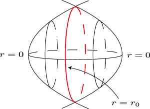
(a)

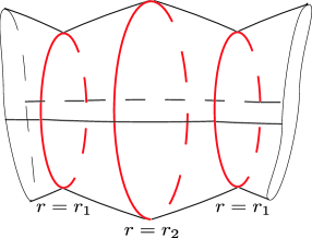
(b)

Figure 1: Schematic diagrams of brane instantons. We construct instanton solutions by gluing two copies of a finite patch of a bulk spacetime with a brane boundary by use of the junction condition. The thick vertical circle at $r=r_{i}(i=0,1,2)$ represents the 4-dimensinal maximally symmetric brane at which the two identical 5-dimensional bulk spaces are glued.

Since we are looking for an instanton solution, we assume a highly symmetric Euclidean spacetime, whose metric is given by

$$ds^{2}_{E}=dr^{2}+b(r)^{2}\gamma_{\mu\nu}dx^{\mu}dx^{\nu},$$ (2)

where $\gamma_{\mu\nu}$ is the metric of 4-dimensional maximally symmetric pace, which is classified into three types by the signature of curvature, i.e., $k=$0 (zero), 1 (positive), or $-1$ (negative). These correspond to the curvature sign of the Friedmann universe after creation. Since the Euclidean space must be compact when we discuss its creation, in the case of $k$=0 or $-1$, we have to make a space compact by identification. Then the flat spacetime is a 4-dimensional torus, and that with $k=-1$ has a more complicated topology.

The equations of motion with these ansatz are given by

$$(b^{\prime})^{2}=k+\frac{1}{12}b^{2}\left(\frac{1}{2}(\phi^{\prime})^{2}-V(\phi)\right),$$ (3)

$$b^{\prime\prime}=-\frac{1}{12}b\left[\frac{3}{2}(\phi^{\prime})^{2}+V(\phi)+2\lambda_{(i)}(\phi)\delta(r-r_{i})\right],$$ (4)

$$\phi^{\prime\prime}+4\frac{b^{\prime}}{b}\phi^{\prime}=\frac{dV}{d\phi}+\frac{d\lambda_{(i)}(\phi)}{d\phi}\delta(r-r_{i}),$$ (5)

where the prime denotes the derivative with respect to $r$, and $k$ is a curvature of the brane.

In what follows, we specify the form of a scalar field potential. We assume that the bulk potential for a scalar field and the tension of the $i$-th brane are given by

$$V(\phi) = \left(\beta^{2}-\frac{2}{3}\right)v^{2}e^{-2\beta\phi},$$ (6)

$$\lambda_{i}(\phi) = \pm 2\sqrt{2}ve^{-\beta\phi},$$ (7)

where $v(>0)$ describes a typical energy scale, and $\beta$ is a parameter of the model Cvetic-Lu-Pope01 ; kobayashi-koyama02 . The signature of Eq. (7) corresponds to the sign of tension of a brane.

This form includes the Randall-Sundrum model ($\beta=0$) and the 5-dimensional effective model derived from M-theory via the Hor̆ava-Witten theory by Lukas, Ovrut and Waldram ($\beta=1$) Lukas-Ovrut-Waldram99 . If we assume supersymmetry and the super potential given by an exponential potential, we find the above forms of a scalar field potential in a bulk and a tension on a brane. Hence, our ansatz is rather generic in the context of a supersymmetric theory. This form of potential has also been used in Cvetic-Lu-Pope01 ; kobayashi-koyama02 .

By using the above potential and tension, we rewrite our basic equations. The equations of motion in the bulk are

$$(b^{\prime})^{2}=k+\frac{1}{12}b^{2}\left[\frac{1}{2}(\phi^{\prime})^{2}-\left(\beta^{2}-\frac{2}{3}\right)v^{2}e^{-2\beta\phi}\right],$$ (8)

$$b^{\prime\prime}=-\frac{1}{12}b\left[\frac{3}{2}(\phi^{\prime})^{2}+\left(\beta^{2}-\frac{2}{3}\right)v^{2}e^{-2\beta\phi}\right],$$ (9)

$$\phi^{\prime\prime}+4\frac{b^{\prime}}{b}\phi^{\prime}=-2\beta\left(\beta^{2}-\frac{2}{3}\right)v^{2}e^{-2\beta\phi}.$$ (10)

Eqs. (9) and (10) are dynamical equations, while Eq. (8) is a constraint equation.

On each brane, we have to impose a boundary condition. Here we assume $Z_{2}$ symmetry on each brane as a conventional brane world model. If we adopt a different condition, our result may be changed.

From $Z_{2}$ symmetry, we have jump conditions for $b^{\prime}$ and $\phi^{\prime}$ on each brane as

$$b^{\prime}(r_{i}) = \mp\epsilon_{i}\frac{\sqrt{2}}{6}b(r_{i})ve^{-\phi}\Bigm{|}_{r=r_{i}},$$ (11)

$$\phi^{\prime}(r_{i}) = \mp\epsilon_{i}\sqrt{2}ve^{-\phi}\Bigm{|}_{r=r_{i}}\,,$$ (12)

where the upper (lower) sign applies to the first boundary at $r=r_{1}$ (the second boundary at $r=r_{2}$) and $\epsilon_{i}=\pm 1$ corresponds to the sign of tension of the $i$-th brane. For a single-brane model, we take the lower sign.

For a single-brane model, we also have to impose another boundary condition at $r=0$. Here we adopt the “no boundary boundary condition” Hartle-Hawking83 . This condition comes from regularity of the 5-dimensional geometry. For $k=1$, it simply gives the boundary condition of $b(0)=0$, $b^{\prime}(0)=1$, $\phi^{\prime}(0)=0$. However, for $k=0$ and $k=-1$, the same boundary condition does not give a regular spacetime. Hence we may have to impose a different boundary condition such as $b(0)\neq 0$, $b^{\prime}(0)=0$ with identification at $r=0$. That is, we have to consider 5-dimensional compactified manifold with different topology from that in Fig. 1(a) such as a 5-dimensional inhomogeneous torus with a brane at $r=r_{0}$. In this paper, we just focus on instanton solutions with topology shown in Fig. 1(a). For instanton solutions with a different topology, we will analyze in a separated paper.

Although the condition $b(0)=0$ for $k=0$ and $k=-1$ causes a singularity as mentioned above, we may be able to construct a singular instanton such as the Hawking-Turok instanton Hawking-Turok98 . Then we also discuss a singular instanton in this paper.

Before constructing an instanton solution, we show that a brane must be flat. The constraint equation (8) should be satisfied for any point $r$, and the boundary conditions (11) and (12) should be also satisfied at the position of a brane ($r=r_{i}$). Substituting Eqs. (11) and (12) into Eq. (8), we find that $k$ must vanish. Therefore, we construct only an instanton solution with a flat brane. This condition, $k=0$, may be understood from the following fact. In the present model, the effective cosmological constant on the brane is given by

$${}^{(4)}\Lambda=\frac{1}{4}\left[V(\phi)+\frac{1}{12}\lambda(\phi)^{2}-\frac{1}{8}\left(\frac{d\lambda(\phi)}{d\phi}\right)^{2}\right]\,,$$ (13)

(see Maeda-Wands00 ). Substituting our potential form (6) and tension (7) into Eq. (13), we find that the effective 4-dimensional cosmological constant vanishes. Therefore the brane should be flat. This is because of supersymmetry. In what follows, we restrict our analysis to a flat-brane model.

III FLAT-BRANE INSTANTON

In this section, we present flat-brane instantons. We discuss a two-brane model and a single-brane one separately.

III.1 Two-brane instanton

Here we construct a two-brane instanton solution. We solve the equations of motion in the bulk, i.e., Eqs. (9) and (10). The solutions are given by

$$b(r)=b_{0}r^{\frac{1}{6\beta^{2}}},$$ (14)

$$\phi(r)=\frac{1}{\beta}\ln\left(\sqrt{2}v\beta^{2}r\right).$$ (15)

When the tension of the first brane is negative and the second brane is positive, respectively, this bulk solution satisfies the jump conditions (11) and (12) at any point $r$. In other words, the positions of branes are freely chosen. We could put branes anywhere we prefer. This is because branes are flat (no curvature).

In order to find the most preferable positions of branes, we evaluate the Euclidean action (1). The Euclidean action (1) is rewritten using equations of motion (8-9) as

$$S_{E} = -\frac{1}{2\kappa^{2}_{5}}\left\{\int_{{\mathcal{M}}}d^{5}x\sqrt{g}\left[\frac{2}{3}V(\phi)\right]\right.$$

$$\left.+\sum_{i}\int_{r=r_{i}}d^{4}x\sqrt{g_{(i)}}\left[\frac{1}{3}\lambda_{(i)}(\phi)\right]\right\}$$

$$= -\frac{V^{\gamma}_{4}}{2\kappa^{2}_{5}}\left\{2\int^{r_{2}}_{r_{1}}drb^{4}(r)\frac{2}{3}V(\phi)\right.$$ (16)

$$\left.+\sum_{i}\frac{1}{3}b^{4}(r)\lambda_{(i)}(\phi)\right\},$$

where $V^{\gamma}_{4}=\int dx^{4}\sqrt{\gamma}$ is the volume of the manifold with a 4-metric $\gamma_{\mu\nu}$. The factor 2 in front of the integral in (16) is required since our instanton solution is constructed by two copies of Euclidean manifolds (see Fig. 1). Performing the integration with solutions (14) and (15), we obtain

$$S_{E} = -\frac{V^{\gamma}_{4}}{2\kappa^{2}_{5}}\frac{b_{0}^{4}}{\beta^{2}}\left\{\frac{2}{3}\left(r_{1}^{\frac{2}{3\beta^{2}}-1}-r_{2}^{\frac{2}{3\beta^{2}}-1}\right)\right.$$ (17)

$$\left.-\frac{2}{3}\left(r_{1}^{\frac{2}{3\beta^{2}}-1}-r_{2}^{\frac{2}{3\beta^{2}}-1}\right)\right\}=0.$$

Unfortunately, this action vanishes and then does not have any minimum (or maximum) with respect to the positions of branes ($r_{1}$ and $r_{2}$). Hence the positions of branes are not determined by the least action principle. This result may be related to the problem of moduli stabilization. We may need some additional mechanism to stabilize the distance between two branes moduli_stabilization .

III.2 Singular single-brane instanton

In this section, we consider the singular instanton such as the Hawking-Turok instanton Hawking-Turok98 . For a single-brane instanton, from the bulk solution (14), we find that $b$ vanishes at $r=0$. At this point, $r=0$, the spacetime curvature of the 5-dimensional manifold diverges and a scalar field also dose so. Therefore this instanton solution has a singularity at $r=0$. However, this singularity is “mild” since the Euclidean action of this instanton solution is finite for some range of $\beta$.

To show it explicitly, we evaluate the Euclidean action. First we divide the action into three terms: $S_{E}^{\rm total}=S_{E}^{\rm bulk}+S_{E}^{\rm brane}+S_{E}^{\rm singularity}$, where $S_{E}^{\rm brane}$ also includes contribution from the Gibbons-Hawking term Gibbons-Hawking77 at the positions of branes. $S_{E}^{\rm singularity}$ is a boundary term at the singularities. Although we do not know an appropriate boundary condition at a singularity, our situation is the same as the case of a 4D singular instanton. For the 4D singular instanton, Vilenkin Vilenkin:1998pp adopted the Gibbons-Hawking term at the singularity. Here we also adopt the Gibbons-Hawking term. We will discuss later on the ambiguity of boundary condition at a singularity.

In order that we perform the integration for $[0,r_{0}]$, first we integrate for an interval $[\varepsilon,r_{0}]$ ($\varepsilon\ll r_{0}$) and we then take a limit of $\varepsilon\rightarrow 0$. The Euclidean action of the bulk is given by

$$S_{E}^{\rm bulk} = -\frac{1}{2\kappa_{5}^{2}}\int_{\mathcal{M}}dx^{5}\sqrt{g}\left[R-\frac{1}{2}\partial_{a}\phi\partial^{a}\phi-V(\phi)\right]$$ (18)

$$= -2\frac{V_{4}^{\gamma}}{2\kappa_{5}^{2}}\lim_{\varepsilon\rightarrow 0}\int_{\varepsilon}^{r_{0}}\frac{2}{3}b(r)^{4}V(\phi)dr$$

$$= \lim_{\varepsilon\rightarrow 0}\frac{V_{4}^{\gamma}}{2\kappa_{5}^{2}}\frac{4b_{0}^{4}}{6\beta^{2}}\left(r_{0}^{\frac{2}{3\beta^{2}}-1}-\varepsilon^{\frac{2}{3\beta^{2}}-1}\right),$$ (19)

where the factor 2 in (18) is required since our instanton contains two copies of the Euclidean manifold (see Fig. 2).

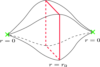
Figure 2: Singular brane instanton. The thick vertical line at $r=r_{0}$ represents the $T^{4}$ brane at which the two identical 5-dimensional bulk spaces are glued. The cross marks at $r=0$ represent singular points.

The brane action is evaluated as

$$S_{E}^{\rm brane} = -\frac{1}{2\kappa_{5}^{2}}\int_{r=r_{0}}dx^{4}\sqrt{g(i)}\left[K^{\pm}_{r=r_{0}}-\lambda_{0}(\phi)\right]$$ (20)

$$= -\frac{V_{4}^{\gamma}}{2\kappa_{5}^{2}}\frac{1}{3}b(r_{0})^{4}\lambda_{0}(\phi)$$

$$= -\frac{V_{4}^{\gamma}}{2\kappa_{5}^{2}}\frac{2}{3\beta^{2}}b_{0}^{4}r_{0}^{\frac{2}{3\beta^{2}}-1}.$$

Finally

The Gibbons-Hawking term at the singularity is given by

$$S_{E}^{\rm singularity} = -2\lim_{\varepsilon\rightarrow 0}\int_{r=\varepsilon}dx^{4}\sqrt{g_{(4)}}\left[\frac{1}{\kappa_{5}^{2}}K\right]$$ (21)

$$= \lim_{\varepsilon\rightarrow 0}\frac{V_{4}^{\gamma}}{\kappa_{5}^{2}}\frac{4b_{0}^{4}}{3\beta^{2}}\varepsilon^{\frac{2}{3\beta^{2}}-1},$$ (22)

where the factor 2 in (21) is also required since this instanton solution has two singularities.

We find that the total action is evaluated as

$$S_{E}^{\rm total}=\frac{V_{4}^{\gamma}}{\kappa_{5}^{2}}\frac{b_{0}^{4}}{\beta^{2}}\varepsilon^{\frac{2}{3\beta^{2}}-1}\Big{|}_{\varepsilon\rightarrow 0}.$$ (23)

If $\beta^{2}\leq 2/3$, this action converges. In that case, our instanton with a singularity could be allowed, which is called a singular instanton.

This action also has no minimum with respect to $r$. Therefore the position of a brane is not fixed, just as the case of a two-brane instanton.

Although we have adopted the Gibbons-Hawking term at the singularity, the boundary condition at the singularity is somewhat ambiguous. For instance, when we consider the action of the asymptorically flat or asymptotically AdS spacetime, we need to add the counter term in order that the action is well-difined Hawking:1995fd ; Kraus:1999di ; Mann:2005yr .

However, in our present model, even if the Gibbons-Hawking term at the singularity is dropped from the action, our result does not be changed significantly. The action converges for $\beta^{2}\leq 2/3$, which is the same condition as the case with the Gibbons-Hawking term. Moreover, when we calculate the quadratic term of the perturbed action (fluctuations around the solution), which will be explicitly shown in next section, it will converges. This guarantees that such an instanton solution is well-defined and harmless, just as the Hawking-Turok instanton is. Therefore we may conclude that our result does not depend on the choice of the boundary condition.

IV Quadratic term of the perturbed action

Here, we investigate perturbations around a singular instanton solution, whose Euclidean action is finite. Although a singular instanton contains a singularity, it is well-defined if fluctuations around the instanton solution do not diverge near singularity. Such an instanton solution could be realized under some circumstance Lavrelashivili98 .

We then calculate the quadratic term of the perturbed action near the singular point. As a useful form of a singular instanton to calculate the variations, we adopt the conformal frame, i.e.,

$$ds^{2}_{E}=b^{2}(R)\left[dR^{2}+\gamma_{\mu\nu}dx^{\mu}dx^{\nu}\right].$$ (24)

Under this coordinate system, the singular instanton solution (Eqs. (14) and (15)) is given by:

$${\rm for}~{}~{}\beta^{2} \neq 1/6,$$

$$b(R) = \tilde{b}_{0}\left[\left(1-\frac{1}{6\beta^{2}}\right)R\right]^{\frac{1}{6\beta^{2}-1}}\,,$$ (25)

$$\phi(R) = \phi^{c}_{1}+\frac{6\beta^{2}}{6\beta^{2}-1}\ln\left[\left(1-\frac{1}{6\beta^{2}}\right)R\right]\,,$$ (26)

$${\rm for}~{}~{}\beta^{2} = 1/6,$$

$$b(R) = b_{0}e^{b_{0}R},$$ (27)

$$\phi(R) = \phi^{c}_{2}+\frac{1}{\beta}R,$$ (28)

where $\tilde{b}_{0}$, $\phi^{c}_{1}$, and $\phi^{c}_{2}$ are constants. For simplicity, we have introduced new variable $\phi(R)\equiv\sqrt{2}\kappa_{5}\varphi(R)$. Note that the singular point of the instanton corresponds to $R=0$ for $\beta^{2}>1/6$, while $R=-\infty$ for $\beta^{2}\leq 1/6$.

The detailed calculation is given in Appendix A. Here we show just the result. Up to total divergence terms, the quadratic term of the perturbed action (70) is

$$\delta_{2}S_{E}=\frac{1}{2}\int d^{5}x\left[\dot{f}^{2}+f_{|\mu}f^{|\mu}+\frac{\ddot{z}}{z}f^{2}\right],$$ (29)

where a dot ($\dot{~{}}$) denotes the derivative with respect to $R$, a vertical line ($|$)denotes the covariant derivative with respect to $\gamma_{\mu\nu}$, $f\equiv b^{\frac{3}{2}}\left[\delta\varphi+(\dot{\varphi_{0}}/\mathcal{H})\psi\right]$ is a gauge-invariant combination of perturbations of a scalar field and of the metric, and $z\equiv b^{3/2}\dot{\varphi}_{0}/\mathcal{H}$. $\mathcal{H}=\dot{b}/b$ and $\psi$ are the Hubble parameter and one of the scalar modes of metric perturbations (see Eq. (64)), respectively.

For our case,

$$\frac{\ddot{z}}{z} = \frac{3}{4}\frac{5-12\beta^{2}}{(6\beta^{2}-1)^{2}R^{2}}\ \ \ \mbox{for}\ \ \beta^{2}\neq\frac{1}{6}$$ (30)

$$= \frac{9}{4}b_{0}^{2}~{}~{}~{}~{}~{}~{}~{}~{}~{}~{}~{}~{}~{}~{}~{}~{}~{}~{}\mbox{for}\ \ \beta^{2}=\frac{1}{6}.$$ (31)

Eq. (29) is exactly the same as the form of a scalar field in flat spacetime with a $r$-dependent mass $\ddot{z}/z$. Note that $\gamma_{\mu\nu}$ is the metric of 4-dimensional flat space. For $\beta^{2}>5/12$, the “mass” term is negative. Hence we expect that such an instanton is unstable with respect to “time” $r$. However, there might be an instanton solution with different metric ansatz (e.g., with different topology), whose action is lower that of the present solution. Although we may be able to conclude that there is no instanton for $\beta^{2}>5/12$, it is unlikely. Hence, in what follows, we consider only the case of $\beta^{2}\leq 5/12$.

Varying Eq. (29) with respect to $f$, we obtain the equation of motion for $f$:

$$\ddot{f}+\Delta f-(\ddot{z}/z)f=0\,.$$ (32)

The separation of variable, i.e., $f=f_{\ell}(R)Y_{\ell}(x^{\mu})$, gives two ordinary differential equations:

$$(\Delta+\ell^{2})Y_{\ell}=0\,,$$ (33)

$$\ddot{f}_{\ell}-\left(\ell^{2}+\frac{\ddot{z}}{z}\right)f_{\ell}=0\,,$$ (34)

where $\ell$ is an eigen value and $Y_{\ell}$ is its eigen function.

For each eigen mode $\ell$ , the quadratic term of the perturbed action is given by

$$\delta_{2}S_{E}=\frac{1}{2}\int dR\left[\dot{f}_{\ell}^{2}+\ell^{2}+\frac{\ddot{z}}{z}\right]\int d^{4}x~{}Y_{\ell}^{2}.$$ (35)

Analyzing the behavior of $f_{\ell}$ near the singularity, we evaluate this action. For $\beta^{2}>1/6$, toward the singularity ($R\rightarrow 0$), the $\ell^{2}$ term dominates in Eq. (34). Then the regular solution of $f_{\ell}$ behaves as

$$f_{\ell}\propto R^{\frac{3}{2(6\beta^{2}-1)}}.$$ (36)

Inserting this solution into the action (35), we obtain

$$\delta_{2}S_{E}\propto R\ell^{2}+\frac{3C_{1}}{2(6\beta^{2}-1)}R^{\frac{2(2-3\beta^{2})}{6\beta^{2}-1}},$$ (37)

where $C_{1}$ is an integration constant. Near the singularity ($R\rightarrow 0)$, (37) is finite if $1/6<\beta^{2}\leq 2/3$.

For $\beta^{2}<1/6$, near singularity ($R\rightarrow-\infty$), the $\ddot{z}/z$ term dominates in Eq. (34). The regular solution of $f_{\ell}$ behaves as

$$f_{\ell}\propto e^{\omega R},$$ (38)

where $\omega^{2}=\ell^{2}$. We also find the same form of the solution for $\beta^{2}=1/6$ if we set $\omega^{2}=\ell^{2}+9b_{0}^{2}/4$.

Near the singularity ($R\rightarrow-\infty$), the integration gives the asymptotic behavior of the action as

$$\delta_{2}S_{E}\propto 2\omega^{2}e^{2\omega R}.$$ (39)

This is finite near singularity.

We conclude that the singular instanton is well-defined for $\beta^{2}\leq 5/12$.

V Toward an inflating-brane instanton

As we have shown in Sec. II, de Sitter brane instanton is not possible for the present potential form and tension (Eqs. (6) and (7)). This is because our potential is based on supersymmetry. However, de Sitter brane may be preferred from the point of view of cosmology. Supersymmetry is also broken in the present universe. Hence, in this section, we examine other potentials which contain some correction terms. Such corrections may be expected from quantum effects via SUSY breaking process. They may provide us an inflating-brane instanton dS_instanton .

To be concrete, we consider the model with the following tension:

$$\lambda=\pm(2\sqrt{2}ve^{-\beta\phi}+\lambda_{i}),$$ (40)

where $\lambda_{i}$ is regarded as a vacuum energy on the $i$-th brane, e.g., the vacuum energy of quantum matter fields on the brane. We assume $\lambda_{i}$ is independent of a scalar field $\phi$. Another model we discuss is the one with the tension such that

$$\lambda=\pm 2\sqrt{2}\alpha ve^{-\beta\phi},$$ (41)

where $\alpha$ describes a deviation from the tension of the original model (7). This model is equivalent to the model with a modified bulk potential. In fact, when we perform the transformation such that $v\rightarrow v/\alpha$ and $\alpha\rightarrow[(\beta^{2}-2/3)/(\beta^{2}-2/3+\delta)]^{1/2}$, we find that the model (41) is the same as the model with the bulk potential $V=(\beta^{2}-2/3+\delta)\exp[-2\beta\phi]$, where $\delta$ is a deviation from the original bulk potential Koyama-etal .

This two modifications give non-vanishing cosmological constant on the brane. For some range of parameters $\lambda_{i}$ and $\alpha$ (e.g., $\lambda_{i}>0$ or $\alpha<1$), we find a positive cosmological constant, which guarantees existence of de Sitter solution on the brane.

First we discuss the case of the tension (40). The junction condition in this case is

$$b^{\prime}(r_{i}) = \frac{b}{12}\left(2\sqrt{2}ve^{-\beta\phi}+\lambda_{i}\right)$$ (42)

$$\phi^{\prime}(r_{i}) = \sqrt{2}v\beta e^{-\beta\phi}.$$ (43)

When we define the new variable

$$J\equiv\phi^{\prime}-\sqrt{2}v\beta e^{-\beta\phi}\,,$$ (44)

the junction condition for a scalar field is given by $J=0$ at $r=r_{i}$. Using the equations of motion (8)-(10) and the junction condition (43), the derivative of $J$ with respect to $r$ at $r=r_{i}$ is given by

$$J^{\prime}(r_{i}) = -\frac{4}{3}\beta v^{2}e^{-2\beta\phi}\left(1+\frac{18}{b^{2}v^{2}}e^{2\beta\phi}\right)^{1/2}$$ (45)

$$+\frac{4}{3}\beta v^{2}e^{-2\beta\phi}\Bigm{|}_{r=r_{i}}<0.$$

$J^{\prime}$ is always negative at the position of brane. This means that $J=0$ is satisfied on either the brane at $r=r_{1}$ or at $r=r_{2}$. Hence, if $J=0$ on one brane, e.g., $r_{1}$, then we cannot impose $J=0$ on the other brane ($r_{2}$). This means that we cannot construct two-brane instanton in this model. For a single brane model, we find $J<0$ at $r=0$ from no boundary boundary condition. $J=0$ is not satisfied at any position of the brane.

Next we consider the model with tension (41). Then the junction condition is given by

$$b^{\prime}(r_{i})=\frac{\sqrt{2}}{6}\alpha ve^{-\beta\phi}\Bigm{|}_{r=r_{i}}$$ (46)

$$\phi^{\prime}(r_{i})=\sqrt{2}\alpha ve^{-\beta\phi}\Bigm{|}_{r=r_{i}}.$$ (47)

We rewrite this condition as follows:

$$b^{\prime}(r_{i}) =\frac{1}{6\beta}\phi^{\prime}(r_{i})b(r_{i})$$ (48)

$$\phi^{\prime}(r_{i}) =\sqrt{2}\alpha ve^{-\beta\phi}\Bigm{|}_{r=r_{i}}.$$ (49)

Defining a new variable $W$ by

$$W\equiv b^{\prime}(r_{i})-\frac{1}{6\beta}\phi^{\prime}(r_{i})b(r_{i})\,,$$ (50)

and using the equations of motion (9) and (10), we obtain the derivative of $W$ with respect to $r$ as

$$W^{\prime}=-3\frac{b^{\prime}}{b}W+\frac{3}{b}\Bigm{|}_{r=r_{i}}.$$ (51)

Since $W=0$ at the position of the brane ($r=r_{i}$), $W^{\prime}$ is always positive. We cannot construct a two-brane instanton solution, because $W=0$ and $W^{\prime}>0$ are not satisfied at both boundaries ($r=r_{1},r_{2}$) simultaneously. For a single-brane model, $W=1$ at $r=0$ from no boundary boundary condition. In this case $W=0$ is not also satisfied because $W^{\prime}>0$ at any position of brane ($W=0$).

As we have shown above, we cannot construct a de Sitter (inflating) brane instanton for the present types of modification. We may need different type of correction terms.

VI CONCLUSION

We have presented instanton solutions in the model with a bulk scalar field. For an exponential potential of a bulk scalar field and tension, which includes Randall-Sundrum model ($\beta=0$) and the 5-dimensional effective Hor̆va-Witten theory ($\beta=1$), we construct flat brane instanton solutions; one is a brane instanton solution with two flat branes, and the other is that with a single brane. We find that a single brane instanton always has a singularity. However, the Euclidean action of such an instanton is finite. As a result, this singular instanton could be realized just as the Hawking-Turok singular instanton. In order to guarantee that the instanton is well-defined, we also analyze the behaviour of the action perturbed around the singular instanton. We find that the quadratic term of the perturbed action is finite if $\beta^{2}<2/3$. This guarantees the singular instanton is well-defined. The second variation equation of the perturbed action is the same form as that of a scalar field in flat spacetime with “time ($R$)”-dependent mass. For $\beta^{2}>5/12$, this mass term becomes negative, which probably means that the instanton is unstable. We then conclude that a singular single-brane instanton is possible if $\beta^{2}\leq 5/12$.

The action of the instanton solutions does not have any minimum with respect to the positions of branes. Then we cannot adopt the least action principle to predict the initial state of a brane universe.

Taking into account some quantum corrections for a bulk potential or tension via SUSY breaking process, we have also investigated possibility of de Sitter brane instanton solution. However, we could not find appropriate instanton solutions. In order to obtain de Sitter brane instanton, we may need to include other important effects, such as the Casimir energy, which are not take into account here, or higher curvature correction terms discussed in Aoyanagi-Maeda04 .

For a flat brane instanton we constructed, we have to consider the evolution of the brane universe after its creation. We may not need inflation just after creation Linde , or may have the KKLMMT type inflation KKLMMT . These issues are left to future study.

Appendix A Quadratic term of the perturbed action

We begin with the original Euclidean action:

$$S_{E}=-\int d^{5}x\sqrt{g}\left[\frac{1}{2\kappa_{5}^{2}}R-\frac{1}{2}\nabla_{a}\varphi\nabla^{a}\varphi-V(\varphi)\right].$$ (52)

We perturb metric and a scalar field as

$$g_{ab}=g^{(0)}_{ab}+h_{ab},~{}~{}~{}~{}~{}\varphi=\varphi_{0}+\delta\varphi.$$ (53)

We then expand the total action until second order perturbations as

$$\delta_{2}\left(\sqrt{g}R\right)=\sqrt{g^{(0)}}\left\{h^{a}_{c}h^{cb}-\frac{1}{2}hh^{ab}+(\frac{1}{8}h^{2}-\frac{1}{16}h^{c}_{d}h^{d}_{c})g^{(0)ab}\right\}R^{(0)}_{ab}$$

$$-\sqrt{g^{(0)}}\left(h^{ab}-\frac{1}{2}hg^{(0)ab}\right)\delta R_{ab}+\sqrt{g^{(0)}}g^{(0)ab}\delta^{2}R_{ab},$$ (54)

where

$$\delta R_{ab}=\delta\Gamma^{c}_{ab;c}-\delta\Gamma^{c}_{ac;b}+2\left(\delta\Gamma^{c}_{ad}\delta\Gamma^{d}_{cb}-\delta\Gamma^{d}_{dc}\delta\Gamma^{c}_{ab}\right),$$ (55)

$$\delta^{2}R_{ab}=\delta^{2}\Gamma^{c}_{ab;c}-\delta^{2}\Gamma^{c}_{ac;b}+\delta\Gamma^{d}_{cd}\delta\Gamma^{c}_{ab}-\delta\Gamma^{d}_{cb}\delta\Gamma^{c}_{ad},$$ (56)

and

$$\delta\Gamma^{c}_{ab}=\frac{1}{2}\left\{h^{a}_{\ c;b}+h_{\ b;a}^{c}-h_{ab}^{\ \ \ c}\right\}.$$ (57)

$$\delta^{2}\left(\sqrt{g}R\right) = \sqrt{g^{(0)}}\left[\left(h^{ac}h_{c}^{\ b}-\frac{1}{2}hh^{ab}\right)R^{(0)}_{ab}+\left(\frac{1}{8}h^{2}-\frac{1}{4}h_{cd}h^{cd}\right)R^{(0)}\right.$$ (58)

$$\left.+\frac{1}{4}\left(2h^{ab;c}h_{ac;b}-h^{ab;c}h_{ab\;c}-2h^{ab}_{\ \ \ ;b}h_{;a}+h_{;a}h^{;a}\right)\right].$$

$$\delta^{2}\left(\sqrt{g}\left[-\frac{1}{2}g^{ab}\partial_{a}\varphi_{0}\partial_{b}\varphi_{0}-V(\varphi_{0})\right]\right)$$ (59)

$$= \sqrt{g^{(0)}}\left[\left(-\frac{1}{2}h^{a}_{\ c}h^{cb}+\frac{1}{4}hh^{ab}\right)\partial_{a}\varphi_{0}\partial_{b}\varphi_{0}+\left(\frac{1}{8}h^{2}-\frac{1}{4}h_{cd}h^{cd}\right)\left(-\frac{1}{2}g^{(0)ab}\partial_{a}\varphi_{0}\partial_{b}\varphi_{0}-V(\varphi_{0})\right)\right.$$

$$\left.-\frac{1}{2}g^{(0)ab}\partial_{a}\delta\varphi\partial_{b}\delta\varphi+\left(h^{ab}-\frac{1}{2}hg^{(0)ab}\right)\partial_{a}\varphi_{0}\partial_{b}\delta\varphi-\frac{1}{2}h\frac{dV}{d\varphi}\Bigm{|}_{0}\delta\varphi-\frac{1}{2}\frac{d^{2}V}{d\varphi^{2}}\Bigm{|}_{0}\delta\varphi^{2}\right]$$

With the metric ansatz (24), a background spacetime is given by the equations of motion:

$$\mathcal{H}^{2}-\dot{\mathcal{H}}-k=\frac{\kappa^{2}_{5}}{3}\dot{\varphi}_{0}^{2},$$ (60)

$$\dot{\mathcal{H}}+\mathcal{H}^{2}-k=-\frac{\kappa^{2}_{5}}{6}\left[\dot{\varphi}_{0}^{2}+2b^{2}V(\varphi_{0})\right],$$ (61)

$$\ddot{\varphi}_{0}+3\mathcal{H}\dot{\varphi}_{0}-b^{2}V_{,\varphi}(\varphi_{0})=0,$$ (62)

where a dot denotes the derivative with respect to $R$, $k$ is the curvature of the brane, and $\mathcal{H}=\dot{b}/b$ is the “Hubble” parameter. Using these equations, the second order variation is given by

$$-\frac{1}{2\kappa_{5}^{2}}\delta^{2}\left(\sqrt{g}R\right)-\delta^{2}\left(\sqrt{g}\left[-\frac{1}{2}g^{ab}\partial_{a}\varphi\partial_{b}\varphi-V(\varphi)\right]\right)$$

$$=-\sqrt{g^{(0)}}\left[-\frac{1}{8\kappa^{2}}\left(h^{2}-2h_{cd}h^{cd}\right)\frac{1}{b^{2}}\left(\dot{\mathcal{H}}+3\mathcal{H}^{2}-3k\right)+\frac{1}{8\kappa^{2}}\left(2h^{ab;c}h_{ac;b}-h^{ab;c}h_{ab;c}-2h^{ab}_{\ \ \ ;b}h_{;a}+h_{;a}h^{;a}\right)\right.$$

$$~{}~{}~{}~{}~{}~{}~{}~{}~{}~{}~{}~{}~{}~{}~{}~{}~{}~{}\left.-\frac{1}{2}g^{(0)ab}\partial_{a}\delta\varphi\partial_{b}\delta\varphi+\left(h^{ab}-\frac{1}{2}hg^{(0)ab}\right)\partial_{a}\varphi\partial_{b}\delta\varphi-\frac{1}{2}h\frac{dV}{d\varphi}\Bigm{|}_{0}\delta\varphi-\frac{1}{2}\frac{d^{2}V}{d\varphi^{2}}\Bigm{|}_{0}\delta\varphi^{2}\right]$$ (63)

Since scalar, vector and tensor modes of perturbations are decoupled in our model, we focus only on scalar perturbations. The scalar mode of metric perturbations is described as

$$ds^{2}_{E}=b^{2}(R)\left[\left(1+2A)dR^{2}+2B_{|\mu}dx^{\mu}dR+\left\{(1-2\psi)\gamma_{\mu\nu}+2E_{|\mu\nu}\right\}dx^{\mu}dx^{\nu}\right)\right],$$ (64)

where $A$, $B$, $E$, and $\psi$ are metric components of perturbations.

The quadratic term of action for scalar perturbations reads (see Mukhanov-etal92 ; Garriga-etal97 )

$$\delta_{2}S_{E} = -\frac{1}{2\kappa^{2}_{5}}\int d^{5}x\sqrt{\gamma}\left\{b^{3}\left[12\dot{\psi}^{2}+24\mathcal{H}A\dot{\psi}+3(3\mathcal{H}^{2}+\dot{\mathcal{H}})A^{2}-6\psi_{|\mu}(A-\psi)^{|\mu}\right.\right.$$ (65)

$$\left.\left.+2\kappa^{2}_{5}\left(-\dot{\varphi}_{0}\dot{A}\delta\varphi-4\dot{\varphi}_{0}\delta\varphi\dot{\psi}-2Ab^{2}\frac{dV}{d\varphi}\delta\varphi\right)+\kappa^{2}_{5}\left(-\delta\dot{\varphi}^{2}-\delta\varphi_{|\mu}\delta\varphi^{|\mu}-\frac{d^{2}V}{d\varphi^{2}}\delta\varphi^{2}b^{2}\right)\right.\right.$$

$$\left.\left.+6\bigtriangleup(B-\dot{E})\left(\mathcal{H}A-\frac{\kappa^{2}_{5}}{3}\dot{\varphi}_{0}\delta\varphi+\dot{\psi}\right)+k\left(3A^{2}+24A\psi-24\psi^{2}-3(B-\dot{E})\Delta(B-\dot{E})\right)\right]\right.$$

$$\left.+\mathcal{D}_{1}+\mathcal{D}_{2}\right\},$$

where $\mathcal{D}_{1}$ and $\mathcal{D}_{2}$ are a total divergence terms:

$$\mathcal{D}_{1} = {\partial\over\partial R}\left\{b^{3}\left[-4\mathcal{H}A^{2}-8\mathcal{H}A\psi+2\mathcal{H}A\Delta E+16\mathcal{H}\psi^{2}-8\mathcal{H}\psi\Delta E+\mathcal{H}(\Delta E)^{2}-\mathcal{H}B_{|\mu}B^{|\mu}-8\mathcal{H}\psi^{2}+4\mathcal{H}\psi\Delta E\right.\right.$$ (66)

$$\left.\left.-2\mathcal{H}E_{|\mu\nu}E^{|\mu\nu}+A_{|\mu}B^{|\mu}-4\psi\Delta B+\Delta E\Delta B+8\kappa_{5}^{2}\psi\dot{\varphi}_{0}\delta\varphi-2\kappa_{5}^{2}\Delta E\dot{\varphi}_{0}\delta\varphi+2\kappa_{5}^{2}A\dot{\varphi}_{0}\delta\varphi\right]\right\},$$

and

$$\mathcal{D}_{2} = \left\{b^{3}\left[\Delta BB^{|\mu}-2\Delta B\dot{E}^{|\mu}+\Delta\dot{E}\dot{E}^{|\mu}+E^{|\mu\nu\rho}E_{|\nu\rho}-E^{|\rho}_{\ \ |\nu\rho}E^{|\mu\nu}-\dot{A}B^{|\mu}+B^{|\mu\nu}B_{|\nu}-\Delta BB^{|\mu}\right.\right.$$ (67)

$$\left.\left.+4\psi\dot{B}^{|\mu}-\Delta E\dot{B}^{|\mu}+12\mathcal{H}\psi B^{|\mu}-3\mathcal{H}\Delta EB^{|\mu}-6\mathcal{H}AB^{|\mu}+2\kappa_{5}^{2}\delta\varphi\dot{\varphi}_{0}B^{|\mu}\right.\right.$$

$$\left.\left.+k\left(12\psi E^{|\mu}-6AE^{|\mu}-E^{|\mu\nu}E_{|\nu}-2\Delta EE^{|\mu}+3(B-\dot{E})(B-\dot{E})^{|\mu}\right)\right]\right\}_{|\mu}.$$

Here we consider the model with $k=0$ because we obtain only a flat brane solution. By varying Eq. (65) with respect to $(B-\dot{E})$, we get the following constraint equation:

$$\dot{\psi}=\frac{\kappa^{2}_{5}}{3}\dot{\varphi}_{0}\delta\varphi-\mathcal{H}A\ .$$ (68)

We introduce a gauge-invariant combination of perturbations of a scalar field and of the metric Mukhanov-etal92

$$f=b^{\frac{3}{2}}\left[\delta\varphi+(\dot{\varphi_{0}}/\mathcal{H})\psi\right]=b^{\frac{3}{2}}\left[\delta\varphi^{\rm(GI)}+(\dot{\varphi_{0}}/\mathcal{H})\Psi\right],$$ (69)

where $\delta\varphi^{\rm(GI)}$ is the gauge-invariant scalar field perturbation. Using (68) and (69) to replace $\dot{\psi}$ and $\delta\varphi$ with $A$, $\psi$ and $v$, we obtain the following quadratic action:

$$\delta_{2}S_{E}=\frac{1}{2}\int d^{5}x\left[\dot{f}^{2}+f_{|\mu}f^{|\mu}+\frac{\ddot{z}}{z}f^{2}+\mathcal{D}_{1}+\mathcal{D}_{2}+\mathcal{D}_{3}\right],$$ (70)

where $z=b^{\frac{3}{2}}\dot{\varphi}_{0}/\mathcal{H}$ and $\mathcal{D}_{3}$ is a total divergence term:

$$\mathcal{D}_{3} = {\partial\over\partial R}\left\{2b^{\frac{3}{2}}\dot{\varphi}_{0}Af-2b^{3}\frac{\dot{\varphi}_{0}^{2}}{\mathcal{H}}A\psi-\frac{3}{2}\mathcal{H}f^{2}-\frac{\kappa_{5}^{2}}{3}\frac{\dot{\varphi}_{0}^{2}}{\mathcal{H}}f^{2}\right.$$ (71)

$$\left.-2b^{\frac{3}{2}}\frac{\ddot{\varphi}_{0}}{\mathcal{H}}f\psi+2b^{\frac{3}{2}}\dot{\varphi}_{0}f\psi-b^{3}\frac{\dot{\varphi}_{0}^{2}}{\mathcal{H}}\psi^{2}+b^{3}\frac{\dot{\varphi}_{0}\ddot{\varphi}_{0}}{\mathcal{H}^{2}}\psi^{2}-\frac{3b^{2}}{\kappa_{5}^{2}}\frac{\psi_{|\mu}\psi^{|\mu}}{\mathcal{H}}\right\}.$$

This Euclidean action is the same as that of a massive scalar field $f$ with “time ($R$)”-dependent mass term, which is $({\ddot{z}}/{z})f^{2}$, in a 5-dimensional flat Euclidean space.

References

- (1) K. Akama, Lect. Notes Phys. 176, 267 (1982).
- (2) V. A. Rubakov and M. E. Shaposhnikov, Phys. Lett. 152B, 136 (1983).
- (3) J. Polchinski, Phys. Rev. Lett. 75, 4724 (1995).
-
(4)
N. Arkani-Hamed, S. Dimopoulos, and G. Dvali,
Phys. Lett. B429, 263 (1998);
I. Antoniadis, N. Arkani-Hamed, S. Dimopoulos, and G. Dvali, Phys. Lett. B 436, 257 (1998);
N. Arkani-Hamed, S. Dimopoulos and G. Dvali, Phys. Rev. D59, 086004 (1999);
N. Arkani-Hamed, S. Dimopoulos, N. Kaloper, and J. March-Russell, Nucl. Phys. B567, 189 (2000). - (5) L. Randall and R. Sundrum, Phys. Rev. Lett. 83, 4690 (1999).
- (6) L. Randall and R. Sundrum, Phys. Rev. Lett. 83, 3370 (1999).
- (7) P. Binétruy, adn, C. Deffayet, and Langlois, Nucl. Phys.565, 269 (2000).
- (8) T. Shiromizu, K. Maeda, and M. Sasaki, Phys. Rev. D 62, 024012 (2000).
- (9) A. Lukas, B. A. Ovrut, and D. Waldram, Phys. Rev. D 60 086001 (1999).
- (10) K. Maeda and D. Wands, Phys. Rev. D 62, 124009 (2000).
-
(11)
Y. Himemoto and M. Sasaki,
Phys. Rev. D 63, 044015 (2001);
J. Yokoyama and Y. Himemoto, Phys. Rev. D 64, 083511 (2001);
N. Sago, Y. Himemoto, and M. Sasaki, Phys. Rev. D 65, 024014 (2002);
Y. Himemoto, T. Tanaka, and M. Sasaki, Phys. Rev. D 65, 104020 (2002);
Y. Himemoto and T. Tanaka, Phys. Rev. D 67, 084014 (2003);
T. Tanaka and Y. Himemoto, Phys. Rev. D 67, 104007 (2003). -
(12)
K. Koyama and K. Takahashi,
Phys. Rev. D 67, 103503 (2003); ibid. 68,
103512 (2003);
H. Yoshiguchi and K. Koyama, Phys. Rev. D 70, 043513 (2004). - (13) T. Kobayashi and T. Tanaka, Phys. Rev. D 69, 064037 (2004).
- (14) A. Vilenkin, Phys. Lett. 117B, 25 (1982).
- (15) S. Coleman and F. de Luccia, Phys. Rev. D 21, 3305 (1980).
- (16) J. B. Hartle and S. W. Hawking, Phys. Rev. D 28, 2960 (1983).
- (17) W. Israel, Nuovo Cimento Soc. Ital. Fis. B 44, 1 (1966).
- (18) J. Garriga and M. Sasaki, Phys. Rev. D 62, 043523 (2000).
- (19) S. W. Hawking, T. Hetrog, and H. S. Reall, Phys. Rev. D 63, 083504 (2001).
- (20) S. W. Hawking, T. Hetrog, and H. S. Reall, Phys. Rev. D 62, 043501 (2000).
-
(21)
S. Nojiri and S. D. Odintsov,
Phys. Lett. B 484, 119 (2000);
S. Nojiri, S. D. Odintsov, and S. Zerbini, Phys. Rev. D. 62, 064006 (2000). - (22) K. Aoyanagi and K. Maeda, Phys. Rev. D. 70, 123506 (2004).
- (23) S. Nojiri and S.D. Odintsov, J. High Energy Phys. 07, 049 (2000).
- (24) M. Cvetiv̆, H. Lü, and C. N. Pope, Phys. Rev. D 63, 086004 (2001).
- (25) S. Kobayashi and K. Koyama, J. High Energy Phys. 12, 056 (2002).
- (26) S. W. Hawking and N. Turok, Phys. Lett. B 425, 25 (1998).
-
(27)
W. D. Goldberger and M. B. Wise,
Phys. Rev. Lett. 83 4922 (1999);
S. B. Giddings, S. Kachre, and J. Polchinski, Phys. Rev. D 66, 106006 (2002);
I. R. Klebanov and M. J. Strassler, J. High Energy Phys. 08, 052 (2000). -
(28)
G. W. Gibbons and S. W. Hawking,
Phys. Rev. D 15, 2752 (1977);
J. W. York, Phys. Rev. Lett. 28, 1082 (1972). - (29) A. Vilenkin, Phys. Rev. D 57, 7069 (1998)
- (30) S. W. Hawking and G. T. Horowitz, Class. Quant. Grav. 13, 1487 (1996)
- (31) P. Kraus, F. Larsen and R. Siebelink, Nucl. Phys. B 563, 259 (1999)
- (32) R. B. Mann and D. Marolf, arXiv:hep-th/0511096.
- (33) G. Lavrelashvili, Phys. Rev. D 58, 063505 (1998).
- (34) If we include higher curvature terms such as Gauss-Bonnet term, which are also expected to exist as quantum correction terms, we can construct de Sitter-brane instanton. See Aoyanagi-Maeda04
-
(35)
A. Linde,
JCAP 0410, 004 (2004);
A. Linde, J. Phys. Conf. Ser. 24 151 (2005). - (36) S. Kachru, R. Kallosh, A. Linde, J. Maldacena, L. McAllister, and S. P. Trivedi, JCAP 0310, 013 (2003).
- (37) V. F. Mukhanov, H. A. Feldmann, and R. H. Brandenberger, Phys. Rep. 255, 203 (1992).
- (38) J. Garriga, X. Montes, M. Sasaki, and T. Tanaka, Nucl. Phys. B513, 343, (1998).