Duality-Symmetric Approach to General Relativity and Supergravity

Duality-Symmetric Approach
to General Relativity and Supergravity

Alexei J. NURMAGAMBETOV A.J. Nurmagambetov

A.I. Akhiezer Institute for Theoretical Physics, NSC “Kharkov Institute of Physics
and Technology”, 1 Akademicheskaya Str., Kharkiv, 61108 Ukraine

ajn@kipt.kharkov.ua

Received October 19, 2005, in final form February 03, 2006; Published online February 15, 2006

We review the application of a duality-symmetric approach to gravity and supergravity with emphasizing benefits and disadvantages of the formulation. Contents of these notes includes: 1) Introduction with putting the accent on the role of dual gravity within M-theory; 2) Dualization of gravity with a cosmological constant in ${\rm D}=3$; 3) On-shell description of dual gravity in ${\rm D}>3$; 4) Construction of the duality-symmetric action for General Relativity with/without matter fields; 5) On-shell description of dual gravity in linearized approximation; 6) Brief summary of the paper.

duality; gravity; supergravity

83E15; 83E50; 53Z05

To memory Vladimir G. Zima and Anatoly I. Pashnev, my colleagues and friends, whom I had a privilege to know, and who I now miss.

1 Introduction

We are living in an epoch of Duality. Starting at the first half of the last century with Quantum Mechanics, solid states and condensed matter physics, Duality was recognized at early 70th as a very useful tool in studying high energy physics of strong interactions. Later on, Duality was successfully applied for developing non-perturbative methods in QCD. Other interesting observations on Duality in supergravities and perturbative String theory lent credence to Duality as a key ingredient of a Unified Theory, whatever it would be.

A most promising way we could follow in our quest for a Unified Theory is the Superstring theory [52, 66, 90]. However, the initial success in the development of string theory after the “First Superstring revolution” revealed a drawback, when at the end of 80th it was understood that the map of perturbative Superstring theory looks like

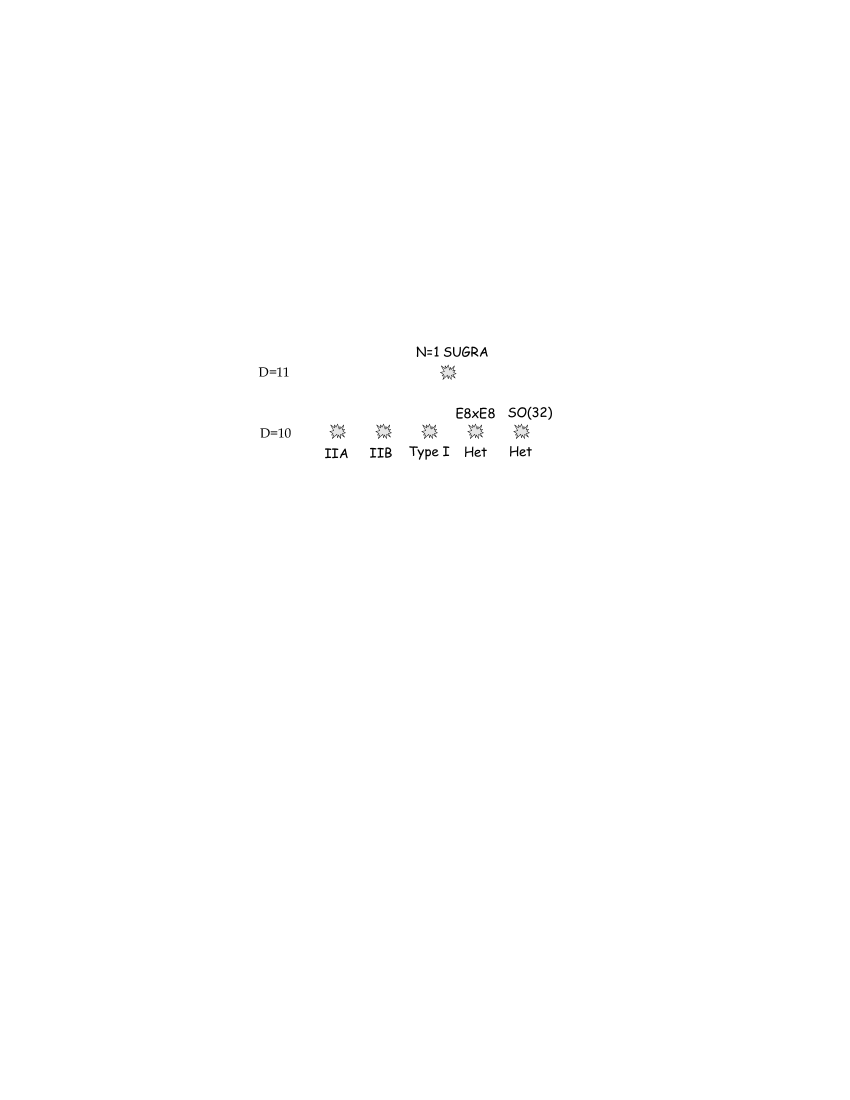
Figure 1: Strings’ Theory map before the “Second Superstring Revolution”.

Clearly, this picture demonstrated a very strange and unexpected feature of the String theory such as having five consistent ten-dimensional Unified Theories instead of a naively expected and desirable one Theory of Everything. Many questions were also addressed to the role of eleven-dimensional supergravity in the picture, since it was hardly related to any Strings, and its interpretation within Superstring theory was obscured. These and other related problems of String theory were resolved with discovering different kinds of Dualities between String theories in weak and strong coupling constant regimes [60]. As a result, the map of String theories was modified to

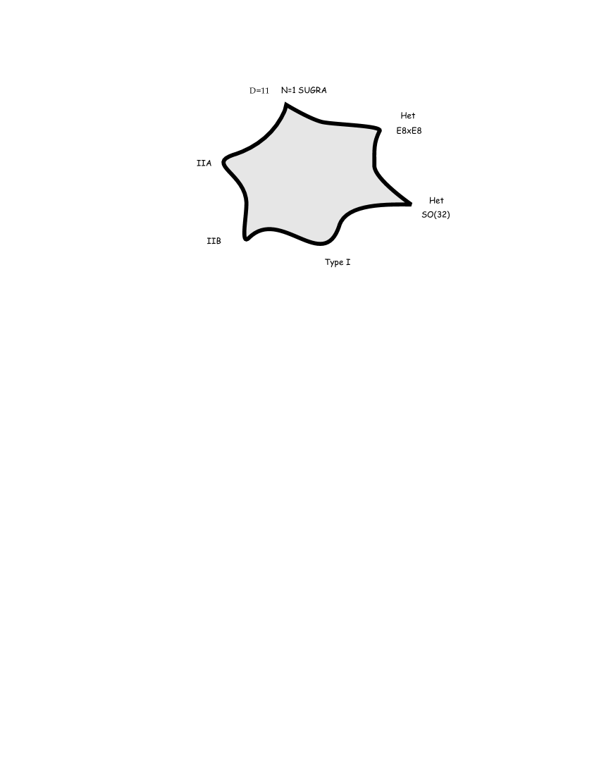
Figure 2: M-theory map.

The heart of the non-perturbative unification of String theories was christened M-theory. During the last decade M-theory was under the active studying, but one should ascertain that our knowledge of M-theory structure is still far from complete. Curiously enough, we had more strong evidence on conjectured time ago quantum symmetries of M-theory such as U-duality [84], having for the time being no classical M-theory description which would contain classical U-duality as a symmetry group. We can also discuss a Landscape of all possible vacua of M-theory [98, 44], bearing in mind at the same time a Landscepticism to this approach [8]. We can find various scenario of appearing the de Sitter phase in M-theory Cosmology [68], having nowadays no good mechanism of supersymmetry breaking and a solution to the cosmological constant problem. We have known the spectrum of free higher-spin fields in String theory, but it is not clear to date how to extract from M-theory a detailed information on higher-spin fields interactions. One can continue this list of potential problems of M-theory, and most of these problems are indications that little is known on a microscopic formulation of M-theory.

The role of eleven-dimensional supergravity [26] in M-theory picture becomes transparent: it is the low-energy limit of M-theory. In its turn, ten-dimensional supergravities [92] correspond to the low-energy limits of different superstrings when strings tension goes to infinity. Many initial conjectures on dualities between string theories and M-theory were successfully proved for corresponding supergravities. And vice versa, many substantial fragments of Dualities in supergravities were regained for Strings.

Though Supergravity has been approved as a very useful tool in studying M-theory, such an approach is apparently restrictive. The field content of (ungauged) ${\rm D}=10$ supergravities consists only of massless fields which form the bottom of the whole spectrum of superstrings’ excitations. The total number of superstring modes is infinite, and other fields of Superstring spectrum are massive, with masses of an order of the Plank mass. Clearly, these fields are too heavy to include it in Supergravity as a low-energy effective theory constructed out of light fields. However, in the opposite to the low energy limit the string tension goes to zero, all the String modes become massless, and we are going to tell on the high energy limit of String theory, where the full hidden symmetry of String theory is restored. (To make the discussion on various limits of String theory more transparent to the reader we add the corresponding Appendix.) An effective field theory which will describe the high energy limit of String theory and will manifestly be invariant under the full symmetry of String theory has to deal with infinite set of massless higher-spin fields, and shall be a dual to Supergravity theory [53]. The strong coupling limit of String theory could be obtained then via the hidden symmetry breaking upon coming from ultra-high energies to the Plank energy. Hence, figuring out the full hidden symmetry structure will supply us with an important information on the effective action of String theory in the strong coupling regime.

So far we did not specify the String theory we will consider in the strong coupling regime. However, the strong coupling limit of type IIA superstring theory is precisely M-theory [100, 106], so following the way of the reasoning in the above we have to conclude that a symmetry of M-theory shall be big enough to accommodate infinite number of fields: it has to be infinite-dimensional!

An infinite-dimensional algebraic structure is common for Strings. A first quantized (super)string theory is managed by the infinite-dimensional Virasoro algebra [101, 48], which is a particular example of the Kac–Moody algebras [65]. The infinite-dimensional structure of an M-theory symmetry should have an impact on the low-energy effective action. So, we could pose a natural question: how would we observe fragments of this infinite-dimensional symmetry inside of ${\rm D}=11$ supergravity?

A way of producing Kac–Moody structures in Supergravities is known: they come from the toroidal dimensional reduction of ${\rm D}=10/11$ Supergravities. To be precise, the following chain of $\mathrm{E}_{n}$ groups ($\mathrm{E}_{1}\sim R^{+}$, $\mathrm{E}_{2}=\mathrm{A}_{1}$, $\mathrm{E}_{3}=\mathrm{A}_{2}\oplus\mathrm{A}_{1}$, $\mathrm{E}_{4}=\mathrm{A}_{4}$, $\mathrm{E}_{5}=\mathrm{D}_{5}$; see e.g. [84])

$$\mathrm{E}_{1}\longrightarrow\mathrm{E}_{2}\longrightarrow\mathrm{E}_{3}\longrightarrow\mathrm{E}_{4}\longrightarrow\mathrm{E}_{5}\longrightarrow\mathrm{E}_{6}\longrightarrow\mathrm{E}_{7}\longrightarrow\mathrm{E}_{8}$$

appears under dimensional reduction of ${\rm D}=11$ supergravity on

$$T_{1}\longrightarrow T_{2}\longrightarrow T_{3}\longrightarrow T_{4}\longrightarrow T_{5}\longrightarrow T_{6}\longrightarrow T_{7}\longrightarrow T_{8}$$

and these global symmetry groups are in general hidden. To recover such a hidden symmetry structure one should dualize higher-rank fields, with the rank $r>(D-n)/2$, that appear upon the reduction on a n-dimensional torus $T_{n}$ [23, 24, 25].

So far we did not succeed in our quest of a Kac–Moody structure. However, let us take a conjecture that doing the reduction to ${\rm D}=2$ [62, 63, 80], ${\rm D}=1$ [63, 78] and, finally, to ${\rm D}=0$ [76] we will further continue the $\mathrm{E}_{n}$-series like

$$\cdots\longrightarrow\mathrm{E}_{9}\longrightarrow\mathrm{E}_{10}\longrightarrow\mathrm{E}_{11}.$$

Once we accept this, we get what we need, because, algebraically, $\mathrm{E}_{9}$ is the (unique possible) affine extension of $\mathrm{E}_{8}$, and a non-trivial affine extension of any Lie algebra corresponds to a Kac–Moody algebra. The structure of $\mathrm{E}_{10}$, $\mathrm{E}_{11}$ is, of course, more complicated, but anyway this is an extension of the Kac–Moody structure.

Remarkably, it was proved that the conjecture does work, at least when one reduces ${\rm D}=11$ Supergravity to two and to one dimensions, and indeed, $\mathrm{E}_{9}$ and $\mathrm{E}_{10}$ global symmetry algebras appear [80, 74]. Hence, it is very likely that we can expect a still elusive $\mathrm{E}_{11}$ to also appear in the end.

We have sketched out a scheme of appearance of the Kac–Moody algebras inside of Supergravity, but in a reduced theory. It is not a priori obvious that there exists a way to relate algebraic structures of a reduced theory with that of the unreduced theory. But it turned out that it is really possible to identify the global symmetry groups of the dimensionally reduced on $T_{n}$ supergravities to the hidden symmetry group of M-theory [41]. Some observations in favor of such an identification were made in mid 80th [42, 43, 77], and following them it was demonstrated [67] that the “exceptional geometry” of the ${\rm D}=3$ maximal Supergravity admits a re-formulation of ${\rm D}=11$ Supergravity in a $\mathrm{E}_{8}$ invariant way. Put it another way, some of the objects which appear upon the reduction do naturally appear in the unreduced theory.

More evidence in favor of $\mathrm{E}_{11}$ as a hidden symmetry of M-theory was found in [102, 103, 93, 94, 104]. There it was considered a non-linear realization of gravity and of the bosonic sector of maximal supergravities which is based on a generalization of Borisov–Ogievetsky formalism [16, 85]. As well as ${\rm D}=4$ gravity [16, 85], ${\rm D}=11$ supergravity can be realized as to be invariant under an infinite-dimensional group, which is the closure of a $\mathrm{G}_{11}$ invariance group [102] and the conformal group $\mathrm{SO(2,10)}$. The group $\mathrm{G}_{11}$ is formed out of the affine group $\mathrm{IGL(11)}$ extended with the subgroup which is generated by antisymmetric type generators with three and six indices. These new generators correspond to $A_{c_{1}c_{2}c_{3}}$ gauge field of ${\rm D}=11$ supergravity and to its dual partner $A_{c_{1}c_{2}\cdots c_{6}}$, and form a subalgebra.

Being finite-dimensional, $\mathrm{G}_{11}$ is apparently not a Kac–Moody algebra, and its coset representatives (see [102]) are not members of a Borel subgroup of a larger group as it should be for the coset formulation of the dimensionally reduced ${\rm D}=11$ supergravity [24, 25]. A way to overcome this obstacle is to invoke more than just antisymmetric gauge fields duality in the picture and to enlarge $\mathrm{G}_{11}$ with a generator corresponding to a dual to graviton field [103]. Then it turns out that simple roots of a Kac–Moody algebra we seek are those of simultaneously sharing $\mathrm{SL(11)}$

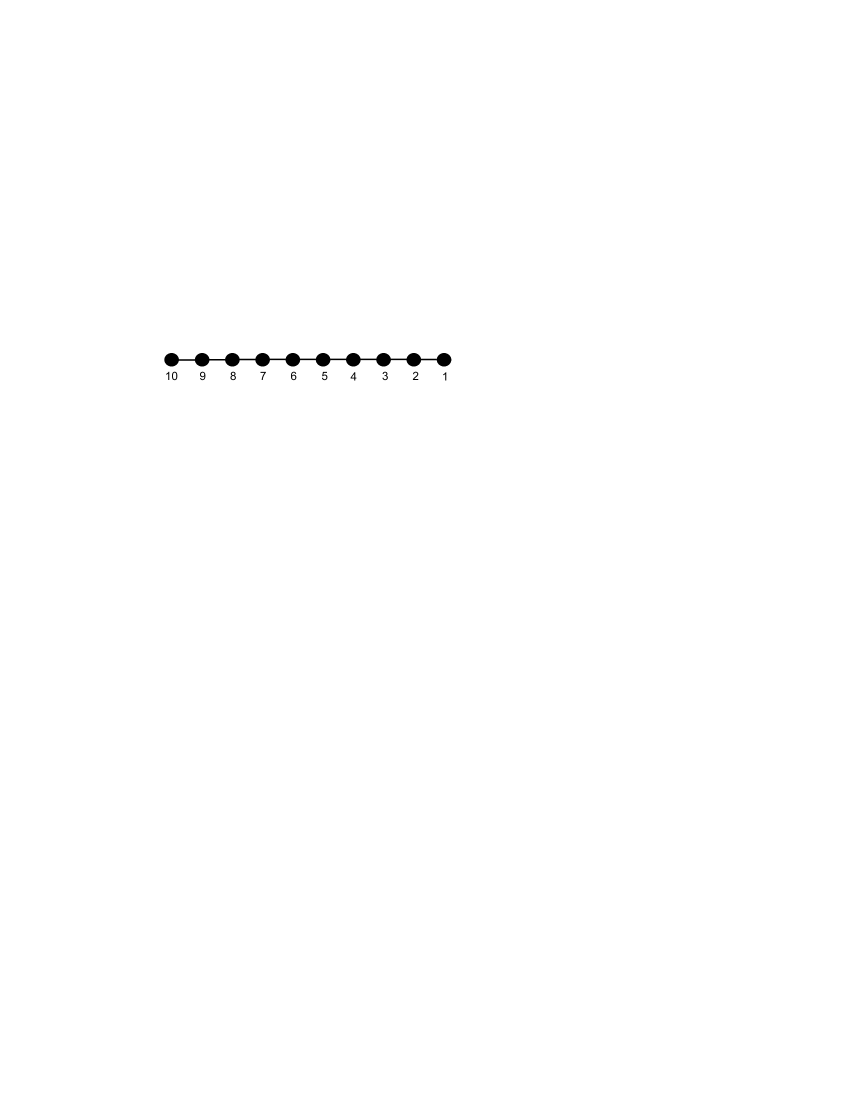
Figure 3: Dynkin diagram of $\mathrm{SL(11)}$.

and $\mathrm{E}_{8}$ subalgebras

Figure 4: Dynkin diagram of $\mathrm{E}_{8}$.

Gluing two Dynkin diagrams together leads to desired $\mathrm{E}_{11}=\mathrm{E}_{8}^{+++}$

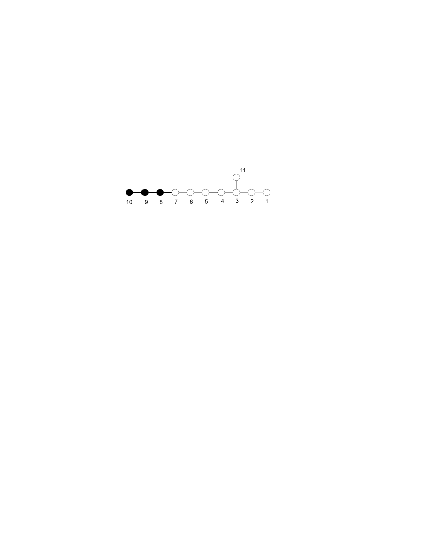
Figure 5: Dynkin diagram of $\mathrm{E}_{11}$.

which is nothing but the extension of the $\mathrm{E}_{8}$ Dynkin diagram with three additional nodes, called the very-extension of $\mathrm{E}_{8}$ [104, 49].

It has to be emphasized that a dual to graviton field was a missing point which should be recovered for the following reasons. From the algebraic point of view, having new generator of the dual to graviton field in a reduced $\mathrm{E}_{11}$ algebra is crucial for recovering the correct algebra for a non-linear realization of type IIA supergravity [104]. This algebra includes generators of fields entering type IIA supergravity multiplet together with generators which correspond to their Hodge dual partners. Hence, a non-linear realization based on this algebra results in a duality-symmetric formulation of type IIA supergravity when fields of the supergravity multiplet and their duals enter the formulation on an equal footing and from the very beginning. In its turn, the structure of $\mathrm{G}_{11}$ dictates the duality-symmetric structure of ${\rm D}=11$ supergravity. Such a duality-symmetric formulation of the antisymmetric gauge field sector was proposed in [5] to couple a dynamical M5-brane [6, 1] to ${\rm D}=11$ supergravity. However, having just duality-symmetric structure of the gauge sector in ${\rm D}=11$ is not enough to recover duality-symmetric structure of type IIA supergravity after reduction [7]. It was straightforward once a dual to graviton field would be taken into account [82], that we are further going to demonstrate.

Any duality-symmetric formulation double physical, i.e. on-shell, degrees of freedom as compared to a standard approach. This mismatch is removed by imposing relations between dual partners, the so-called duality relations. A minimal, but not convenient for further possible applications, way to take duality relations into account is to impose them by hand as an additional part to equations of motion (see e.g. [13]). Following this way, we have to bear in mind that further modifications of equations of motion, such as coupling to external sources, introducing a non-trivial self-interaction of fields, taking into account quantum corrections etc., will require an appropriate change of the duality relations which would be hard in general to guess. More conveniently, but technically more complicated, is to figure out a way to derive duality relations from an action as equations of motion (see [96] for a review). There are many roads to this end; here we will mainly follow [86, 87, 88], reviewing in brief other approaches.

To summarize our Introduction, let us recall that the duality-symmetric structure of ${\rm D}=11$ supergravity is very natural on the way of dynamical realization of $\mathrm{E}_{11}$ conjecture, and if we require the hidden symmetry algebra to be a Kac–Moody-type algebra, we have to figure out a way of dualization of gravity.

The rest of the paper is organized as follows: in the following section we consider a warm-up exercise of dualization of three-dimensional gravity with a cosmological constant. Though this example cannot be considered as a general case, it nevertheless demonstrates some common features of the dualization which will be helpful in further generalization of the dual description to higher dimensions. In Section 3 we construct the on-shell dual gravity in the space-time of dimensions higher than three. Then, in Section 4 we uplift our formulation at the off-shell level. A brief review of the construction in the linearized approximation is given in Section 5, and our conclusions are summarized in the last section. Remarks on the construction, discussion on formulations we use and examples of application are adduced throughout the paper. Our notation and conventions, as well as an informative summary on different limits of String theory, are collected in two Appendices.

2 Dualization of $\boldsymbol{{\rm D}=3}$ gravity

We are getting started with the action of ${\rm D}=3$ gravity with a cosmological constant $\lambda$

$$S=\int d^{3}x\,\sqrt{g}(R+\lambda),$$ (2.1)

and the inclusion of non-zero cosmological constant into the action is important for the subsequent dualization of the model. It will also be convenient for this purpose to present the originally second order action (2.1) in the form of the Hilbert–Palatini first order action

$$S=\int d^{3}x\,\left[\epsilon^{mnk}e_{ka}\left(\frac{1}{2}{R_{mn}}^{bc}\epsilon_{abc}\right)+\lambda\det e^{a}_{m}\right].$$ (2.2)

In the first order formulation a dreibein $e^{a}_{m}$ and $\mathrm{SO(1,2)}$ spin connection $\omega_{m}^{ab}$ are supposed to be independent variables. The curvature tensor depends only on the connection

$${R^{ab}}_{mn}=2\partial_{[m}\omega^{ab}_{n]}+2\omega^{ac}_{[m}\omega^{db}_{n]}\eta_{cd}\equiv\partial_{m}\omega^{ab}_{n}-\partial_{n}\omega^{ab}_{m}+\big{(}\omega^{ac}_{m}\omega^{db}_{n}-\omega^{ac}_{n}\omega^{db}_{m}\big{)}\eta_{cd},$$

where $\eta_{ab}$ is the Minkowski metric tensor with the mostly minus signature (see Appendix A for the notation). As a result, the Einstein equation that comes from the first order action (2.2) is of the first order in the connection. To arrive at the standard second order equation of motion of a spin two bosonic field, one should violate the initial independence of variables and to resolve an algebraic relation between the dreibein and the spin connection. This relation follows from (2.2) when one varies the action over the spin connection as an independent variable. Once the connection is expressed in terms of the dreibeins the standard second order Einstein equation is recovered. Therefore, the dreibeins are the true dynamical variables of the theory, while the spin connection plays the role of an additional but not of a fundamental variable.

However, it is possible to replace vielbeins with other fundamental variables. Let us note to this end that the form of (2.2) suggests the definition of a new connection

$$A^{a}_{m}=\frac{1}{2}\epsilon^{abc}\omega_{mbc}$$

with the same as the dreibeins index structure. In terms of the new variables the curvature tensor acquires the form of a Yang–Mills field strength [89]

$$F^{a}_{mn}=2\partial_{[m}A^{a}_{n]}+\epsilon^{abc}A_{mb}A_{nc}.$$ (2.3)

Then the Hilbert–Palatini action (2.2) becomes

$$S=\int d^{3}x\left[\epsilon^{mnk}e_{ka}F_{mn}^{a}+\lambda\det e^{a}_{m}\right],$$ (2.4)

and it is easy to see that the true equation of motion following from (2.4) upon varying over the dreibein is

$$*F^{ma}+\lambda ee^{ma}=0.$$ (2.5)

We have denoted $e=\det e^{a}_{m}$ in the above and have used the following definition of the dual, with respect to the curved indices, tensor

$$*F^{ma}=\epsilon^{mnk}F^{a}_{nk}.$$

The other equation which can be read off (2.4) is

$${\mathcal{D}}_{m}(\epsilon^{mnk}e_{ka})=0.$$ (2.6)

Here ${\mathcal{D}}_{m}$ is the covariant with respect to $A^{a}_{m}$ derivative, and (2.6) is the algebraic relation which expresses the initially independent variables $A^{a}_{m}$ through $e^{a}_{m}$.

As for the standard first order formulation of gravity in $(e^{a}_{m},\omega^{ab}_{m})$ variables the integrability condition to equations (2.6), (2.5), viz.

$$\mathcal{D}_{m}\mathcal{D}_{n}(\epsilon^{mnk}e_{ka})=0,$$

$$\mathcal{D}_{m}(\ast F^{ma}+\lambda ee^{m}a)=0$$ (2.7)

results in the first-type (for torsion) and in the second-type (for curvature) Bianchi identities respectively. We remind that in the former set of variables these Bianchi identities are ${R^{a}}_{[nkl]}=0$ and $\mathcal{D}_{[m}{R^{ab}}_{nk]}=0$. Note also that taking into account (2.6) the integrability condition (2.7) can be rewritten as

$$\mathcal{D}_{m}(\epsilon^{mnk}F^{a}_{nk})=0,$$ (2.8)

which is nothing but the Bianchi identity for the Yang–Mills field strength (2.3). Strictly speaking, the Bianchi identity (2.8) has nothing to do with the integrability condition (2.7), since it directly follows from the definition (2.3); rather the integrability condition (2.7) is satisfied due to the zero torsion equation (2.6) and the Bianchi identity (2.8).

So far we considered $e^{a}_{m}$ as the fundamental variables. However, we can also think about $A^{a}_{m}$ as the other fundamental variables. To go from one to another we shall use equation (2.5).

Taking the determinant of (2.5) leads to

$$-\det(*F^{ma})=\lambda^{3}e^{2},$$ (2.9)

after that one can resolve (2.5) as

$$e^{ma}=\mp\frac{1}{\lambda\sqrt{-\frac{1}{\lambda^{3}}\det(*F^{ma})}}*F^{ma}.$$ (2.10)

In effect, we have completely determined the dreibein in terms of the dual curvature or, equivalently, in terms of the new connection $A^{a}_{m}$. Substituting this solution to the Lagrangian back results in

$$S=\mp 2\,\mathrm{sign}(\lambda)\int d^{3}x\sqrt{-\frac{1}{\lambda}\det(*F^{ma})}$$ (2.11)

that is the action of the model in terms of $A^{a}_{m}$.

Let us now compare the equation of motion following from (2.11) with equations (2.5) and (2.6). Varying (2.11) with respect to $A^{a}_{m}$ we get the Yang–Mills-type equation of motion (see [89] for details)

$${\mathcal{D}}_{m}\big{(}\sqrt{g}F^{mn}_{a}\big{)}=0$$ (2.12)

on a curved manifold endowed with the metric depending on $A^{a}_{m}$. As it follows from (2.9)

$$\sqrt{g}=\sqrt{-\frac{1}{\lambda^{3}}\det(*F^{ma})}.$$

In addition we have to complete (2.12) with the Bianchi identity (2.8) which follows from the definition of the new curvature (2.3).

One could note that equation (2.12) is nothing but equation (2.6) written down in terms of the new variables when (2.5) is taken into account. In its turn the Bianchi identity (2.8) follows from (2.7) as the integrability condition to the relation (2.5) that is algebraic in this picture. Put it differently an algebraic relation that comes from the action in standard variables becomes the equation of motion of the model in new variables. This phenomenon is a remnant of the dualization, when the Bianchi identities (algebraic relations) of gauge fields become equations of motion of the dual gauge fields. Hence, one can say that (2.11) is the action for gravity in dual variables, or, for short, the dual gravity.

What we can learn from this example? We have observed that the problem is completely resolved in ${\rm D}=3$ case. However, it is only resolved for gravity with a cosmological constant, and the dual Lagrangian is not well defined in the zero cosmological constant limit. Furthermore, the case under consideration cannot be treated as a general case, and the above mentioned way of the dualization is not a general scheme, since gravity in ${\rm D}=3$ possesses the features which cannot be encountered for gravitational theory in other space-time dimensions. For instance, it is the very case where the dualized over SO(1,2) indices connection has the same index structure as the dreibein, and we have used this fact to completely get rid of the dreibeins as fundamental dynamical variables in favor of the dual connection. It would be pertinent to note that using a connection as a fundamental variable is one of the features of the Loop Quantum Gravity (see [79] for a recent review). Also, ${\rm D}=3$ gravity does not have dynamical degrees of freedom  [34, 35, 36], and is interesting rather as a topological exactly (classically and quantum) solvable theory [105].

Taking into account the above, perspectives to generalize such a dual description to higher dimensions do not seem to be so direct. Starting with ${\rm D}=4$ gravity with a cosmological constant we will not have so simple form of equations of motion that would suggest a way of resolving vielbeins in terms of the dual curvature/dual connection. For example, applying the determinant to both sides of the four-dimensional Einstein equation with a cosmological constant does not lead to the dual theory. It results in the Eddington–Schrödinger formulation of gravity [97, 46] which is classically equivalent to the Einstein formulation (see [33, 37] for other treatments of the problem). But even if we were succeed in dualization of higher-dimensional gravity with a cosmological constant it would not be a resolution to the problem in the M-theory context, since there is no place for a cosmological constant in ${\rm D}=11$ supergravity [9].

Finally, we have to emphasize an important point: because of the square root the dual Lagrangian resembles the Nambu–Goto action for strings and branes, it is non-polynomial and it has infinite number of terms with infinite number of derivatives in the small cosmological constant limit $\lambda\rightarrow 0$ supporting with the weak field approximation. In this limit the gravity can be approximated with a small perturbation around Minkowski flat space (it does not contradict the results of [22] since the cosmological constant tends to zero in the limit), and passing to a new curvature through $\ast F^{ma}=\ast F^{mn}e^{a}_{n}$ we get first

$$\det{(\ast F^{ma})}=\det{e^{a}_{m}}\det{(\ast F^{mn})}.$$

Second, we approximate the new curvature as

$$\ast F^{mn}=\Lambda\eta^{mn}+\ast R^{mn},$$ (2.13)

where $\eta^{mn}$ is the inverse to the Minkowski flat metric tensor, and we have fixed for definiteness $\lambda<0$, $\Lambda=|\lambda|$. Also we would like to fix the “minus” sign on the r.h.s. of (2.10), so under these assumptions the Lagrangian for the dual gravity becomes

$$\mathcal{L}=2\sqrt{\frac{1}{\Lambda}\det{e^{a}_{m}}\det{(\ast F^{mn})}}.$$

Substituting (2.13) into the above, we arrive at

$$\mathcal{L}=2\Lambda\sqrt{\det{e^{a}_{m}}}\sqrt{\det{(\delta_{m}^{n}+\frac{1}{\Lambda}\ast R^{n}_{m})}},$$

that after taking into account $\det{M}=\exp{(\mathrm{Tr}\ln M)}$ results in

$$\mathcal{L}=\sqrt{\det{e^{a}_{m}}}\left[2\Lambda+\ast{R^{m}}_{m}-\frac{1}{2\Lambda}\left(\ast R^{mn}\ast R_{mn}-\frac{1}{2}(\ast{R^{m}}_{m})^{2}\right)+\cdots\right].$$

This reminds the situation which one encounters in non-local theories. However, in our example this non-polynomiality appeared because of the choice of dual variables and, as in the case of the Nambu–Goto action, it is harmless. At the same time this observation suggests that in a general case proper non-locality could appear as a by-product of dualization.

3 On-shell dual gravity in $\boldsymbol{\mathrm{D}>3}$: Bianchi vs. Einstein

After an examination of three-dimensional gravity, let us try to figure out a way of proceeding in $\mathrm{D>3}$ case. What we shall find first is a convenient representation of the Einstein equation in a way that allows us to present it as the Bianchi identity for a dual field. It turns out to be convenient for this purpose to write down the Einstein equation in a form which is similar to the dynamics of Maxwell theory with a source.

3.1 Maxwell-like representation of the Einstein equation

To arrive at such a representation let us get started with the Hilbert–Palatini action of $\mathrm{D}$-dimensional gravity

$$S_{HP}=\int_{{\mathcal{M}}^{D}}\hat{R}^{\hat{a}_{1}\hat{a}_{2}}\wedge\hat{\Sigma}_{\hat{a}_{1}\hat{a}_{2}},$$ (3.1)

where

$$\hat{R}^{\hat{a}\hat{b}}=d\hat{\omega}^{\hat{a}\hat{b}}-{\hat{\omega}^{\hat{a}}}_{~{}\hat{c}}\wedge\hat{\omega}^{\hat{c}\hat{b}}$$

is the curvature two-form expressed via $SO(1,D-1)$ connection $\hat{\omega}^{\hat{a}\hat{b}}$ and

$$\hat{\Sigma}_{{\hat{a}}_{1}\cdots{\hat{a}}_{n}}=\frac{1}{(D-n)!}\epsilon_{{\hat{a}}_{1}\cdots{\hat{a}}_{D}}{\hat{e}}^{{\hat{a}}_{n+1}}\wedge\cdots\wedge{\hat{e}}^{{\hat{a}}_{D}}$$

is a $(\mathrm{D}-n)$-form constructed out of vielbeins ${\hat{e}}^{a}$. Since we will use in what follows the reduction of the action to $(\mathrm{D}-1)$-dimensions, we have reserved hats to distinguish $\mathrm{D}$-dimensional indices and variables from $(\mathrm{D}-1)$-dimensional quantities. This notation is generally accepted in the Kaluza–Klein literature, and we will follow it.

Upon varying with respect to the vielbein and the connection we get the Einstein equation of motion

$$\hat{\Sigma}_{{\hat{a}}{\hat{b}}{\hat{c}}}\wedge\hat{R}^{{\hat{b}}{\hat{c}}}=0,$$ (3.2)

and an algebraic relation

$$\hat{\Sigma}_{{\hat{a}}{\hat{b}}{\hat{c}}}\wedge\hat{T}^{\hat{c}}=0,$$

which sets the torsion 2-form $\hat{T}^{\hat{a}}=d\hat{e}^{\hat{a}}-\hat{e}^{\hat{b}}\wedge{{\hat{\omega}}_{\hat{b}}}^{~{}{\hat{a}}}$ to zero. The latter allows expressing the originally independent connection $\hat{\omega}^{{\hat{a}}{\hat{b}}}$ through vielbeins and their derivatives

$${\hat{\omega}}^{{\hat{a}}{\hat{b}}}({\hat{e}})=\frac{1}{2}~{}\hat{e}^{\hat{c}}\left[\hat{e}^{\hat{m}}_{\hat{c}}\hat{e}^{{\hat{n}}{\hat{a}}}\partial_{[{\hat{m}}}\hat{e}_{{\hat{n}}]}^{\hat{b}}-\hat{e}^{\hat{m}}_{\hat{c}}\hat{e}^{{\hat{n}}{\hat{b}}}\partial_{[{\hat{m}}}\hat{e}_{{\hat{n}}]}^{\hat{a}}-\hat{e}^{{\hat{n}}{\hat{a}}}\hat{e}^{{\hat{s}}{\hat{b}}}\partial_{[{\hat{n}}}\hat{e}_{{\hat{s}}]{\hat{c}}}\right].$$ (3.3)

After replacing the connection with (3.3) the Einstein equation is written down in the following form (see [83])

$$d(\hat{\ast}d\hat{e}_{\hat{a}})=\hat{\ast}\hat{\tilde{J}}^{[1]}_{\hat{a}},$$ (3.4)

where a one-form $\hat{\tilde{J}}^{[1]}_{\hat{a}}$ is

$$\hat{\tilde{J}}^{[1]}_{\hat{a}}=(-)^{\frac{D(D-5)}{2}}\hat{J}^{[1]}_{\hat{a}}+\hat{\ast}d\hat{S}^{[D-2]}_{\hat{a}},$$ (3.5)

and

$$\hat{J}^{[1]}_{\hat{a}}=\hat{\ast}\left[\hat{\omega}^{{\hat{b}}{\hat{c}}}({\hat{e}})\wedge d\hat{\Sigma}_{{\hat{a}}{\hat{b}}{\hat{c}}}+(-)^{D-3}~{}{{\hat{\omega}}}^{\hat{b}}_{~{}{\hat{d}}}({\hat{e}})\wedge\hat{\omega}^{{\hat{d}}{\hat{c}}}({\hat{e}})\wedge\hat{\Sigma}_{{\hat{a}}{\hat{b}}{\hat{c}}}\right],$$ (3.6)

$$\hat{S}^{[D-2]}_{\hat{a}}=\hat{\ast}(\hat{e}^{\hat{b}}\wedge\hat{e}_{\hat{a}})~{}\hat{e}^{\hat{m}}_{\hat{c}}\hat{e}^{\hat{n}}_{\hat{b}}\partial_{[\hat{m}}\hat{e}^{\hat{c}}_{{\hat{n}}]}.$$ (3.7)

Two remarks are appropriate here.

Remark 3.1.

Equation (3.4) looks like that of the Maxwell electrodynamics with an electric-type source. This form of the Einstein equation is not a new one; it has been pointed out in literature for a long time (see e.g. [99, 15]). Since the equation is written in terms of differential forms, it is manifestly invariant under general coordinate transformations. But its manifest invariance under local Lorentz rotations is lost. However, the right hand side of (3.4) is a modified Landau–Lifshitz pseudo-tensor, so the non-covariance on the left hand side is compensated by the pseudo-tensor-type transformations on the right hand side. Hence, equation (3.4) is covariant under the general coordinate transformations and the Lorentz rotations in the tangent space.

Remark 3.2.

In the form of (3.4) the Einstein equation is closely related to the so-called “teleparallel” version of General Relativity (see [3] for a review).

As a next step towards realization of our program we have to rewrite the Einstein equation (3.4) as the Bianchi identity of a dual field. The Poincaré lemma claims that in a trivial space-time topology setting one can present the conserved “current” form $\hat{\tilde{J}}^{[1]}_{\hat{a}}$ as the curl of a “pre-current” form

$$\hat{\ast}\hat{\tilde{J}}^{[1]}_{\hat{a}}=d\hat{\ast}\hat{\tilde{G}}^{[2]}_{\hat{a}}.$$ (3.8)

With account of it, the Einstein equation becomes $d(\cdots)=0$ which is the Bianchi identity for a dual field. That is exactly what we need. Therefore, to make the final step from Einstein to Bianchi, we have to resolve (3.8) to find $\hat{\tilde{G}}^{[2]}_{\hat{a}}$.

As to the explicit expression of the “current” (cf. equations (3.5), (3.6), (3.7)) it is not so simple to derive the “pre-current” $\hat{\tilde{G}}^{[2]}_{\hat{a}}$ exactly, and in a local form. Furthermore, there are no general arguments that $\hat{\tilde{G}}^{[2]}_{\hat{a}}$ has always to be a local expression. So it does not become a surprise that a general procedure of resolving (3.8) sacrifices locality and leads to local expressions for “pre-currents” only for “currents” of a special type.

3.2 Resolving via inverse d’Alembertian

To write down equation (3.4) in terms of a (Hodge) dual field one has to introduce the dual field strength

$$\hat{F}_{\hat{a}}=\hat{\ast}d\hat{e}_{\hat{a}},$$

after that the Einstein equation recasts in

$$d\hat{F}_{\hat{a}}=\hat{\ast}\hat{\tilde{J}}^{[1]}_{\hat{a}}.$$ (3.9)

The general solution to an equation

$$dK=\mathcal{J};\qquad\mathcal{J}\neq\mathcal{J}(K),$$ (3.10)

which is presumably the case under consideration, is as follows

$$K=\Box^{-1}{\boldsymbol{\delta}}\mathcal{J}+d\chi.$$ (3.11)

Here ${\boldsymbol{\delta}}=(-)^{(D-p)p-1}\ast d\ast$ is the $D$-dimensional co-derivative operator acting on a $p$-form, $\Box=d{\boldsymbol{\delta}}+{\boldsymbol{\delta}}d$ is the d’Alembertian and $\chi$ is a differential form of the appropriate rank. To verify (3.11) one should notice the Hodge identity

$$d\Box^{-1}{\boldsymbol{\delta}}+{\boldsymbol{\delta}}\Box^{-1}d=1,$$

which is easy to prove with taking into account

$$[d,\Box]=0,\qquad[{\boldsymbol{\delta}},\Box]=0.$$ (3.12)

These relations follow from the d’Alembertian definition. Then, for any form $\Omega$

$$\Omega=1\cdot\Omega=d\big{(}\Box^{-1}{\boldsymbol{\delta}}\Omega\big{)}+{\boldsymbol{\delta}}\big{(}\Box^{-1}d\Omega\big{)},$$ (3.13)

and the last term on the r.h.s. of (3.13) vanishes for a closed form. Thus, the solution (3.11) is the sum of a particular solution to the non-homogeneous differential equation (3.10) and the general solution to the homogeneous equation $dK=0$.

What is a restriction on this approach? If $\mathcal{J}$ is a co-closed form, i.e. ${\boldsymbol{\delta}}\mathcal{J}=0$, or in other words is a zero mode of the d’Alembertian, the way of the reasoning apparently fails. Hence, the current form $\mathcal{J}$ has not to be co-closed.

But what we have to do if nevertheless the current is a co-closed form? In such a case we have to apply a regularization. There are many ways to this end, we will treat it as follows. Recall the following integral representation for a variable $\rho$

$$\frac{1}{\rho^{n}}=\frac{1}{(n-1)!}\int_{0}^{\infty}dt\,t^{n-1}e^{-t\rho},\qquad n>0,$$ (3.14)

which follows from the Euler integral for the gamma-function. This representation can be used to define the inverse d’Alembertian

$$\frac{1}{\Box}\,\psi=\int_{0}^{\infty}dt\,e^{-t\Box}\psi$$ (3.15)

if a (vector-indices) function $\psi$ will be regarded as the sum over the complete set of the d’Alembertian eigenfunctions $\psi_{n}$ with coefficients $\alpha_{n}$

$$\psi=\sum_{n}\alpha_{n}\psi_{n}.$$

By definition

$$\Box\psi_{n}=\lambda_{n}\psi_{n}$$ (3.16)

with eigenvalues $\lambda_{n}$. Then, (3.15) and (3.16) result in

$$\Box^{-1}\psi_{n}=\lambda^{-1}_{n}\psi_{n},$$

and we have to complete the definition of the inverse operator to include the d’Alembertian zero modes. It could for instance be done by replacing the eigenvalues with $\lambda^{\tt reg.}_{n}=\lambda_{n}+\mathfrak{e}(\lambda,n)$ such that $\lambda_{n}+\mathfrak{e}(\lambda,n)\neq 0$ [45], and the regularized d’Alembertian has a well defined inverse operator.

To figure out other features of the method, let us apply the procedure of resolving to a well-known case borrowed for instance from supergravities. A simplest example is the Bianchi identity for ${\rm D}=11$ supergravity gauge field [5, 25] in the zero fermion setting

$$dF^{(7)}=F^{(4)}\wedge F^{(4)};\qquad F^{(4)}=dA^{(3)},\qquad\ast F^{(4)}=F^{(7)}.$$ (3.17)

The r.h.s. of (3.17) is a current form in our jargon, and it is easy to see that the pre-current form is $G^{(7)}=A^{(3)}\wedge F^{(4)}$. Hence the solution to the Bianchi identity is $F^{(7)}=dA^{(6)}+A^{(3)}\wedge F^{(4)}$. Let us now recover this result by use of (3.11). It leads to

$$F^{(7)}=d\chi^{(6)}+\Box^{-1}{\boldsymbol{\delta}}\big{(}F^{(4)}\wedge F^{(4)}\big{)}.$$

Noticing that $F^{(4)}\wedge F^{(4)}=d(A^{(3)}\wedge F^{(4)})$ we have

$$\Box^{-1}{\boldsymbol{\delta}}d\big{(}A^{(3)}\wedge F^{(4)}\big{)}=\Box^{-1}(\Box-d{\boldsymbol{\delta}})A^{(3)}\wedge F^{(4)}=A^{(3)}\wedge F^{(4)}-d\Box^{-1}{\boldsymbol{\delta}}\big{(}A^{(3)}\wedge F^{(4)}\big{)}.\!\!$$

To get the last expression we have used $[\Box^{-1},d]=0$, which comes from (3.12) as

$$[d,\Box]=0\quad\leadsto\quad d=\Box d\Box^{-1}\quad\leadsto\quad\Box^{-1}d=d\Box^{-1}.$$

Finally,

$$F^{(7)}=d\left(\chi^{(6)}-\Box^{-1}{\boldsymbol{\delta}}\big{(}A^{(3)}\wedge F^{(4)}\big{)}\right)+A^{(3)}\wedge F^{(4)}\equiv dA^{(6)}+A^{(3)}\wedge F^{(4)}.$$

The final result is a local expression since any trace of non-locality is hidden with introducing a new field. As a consequence, an appropriate local gauge transformation has to be assigned to $A^{(6)}$ rather than to $\chi^{(6)}$.

We would like to point out that one may encounter an opposite situation when an initially local theory possesses an invariance under special non-local transformations. An example of such transformations is duality rotations in four-dimensional Maxwell theory [39]. A good choice of new variables may help to avoid non-locality as we will see under discussing different approaches to duality-symmetric theories.

3.3 Dual to graviton field and its equation of motion

At this stage we have all necessary tools to accomplish the current task: equation (3.9) is resolved with

$$\hat{F}^{[D-2]}_{\hat{a}}=d\hat{A}^{[D-3]}_{\hat{a}}+\hat{\ast}\hat{\tilde{G}}^{[2]}_{\hat{a}}\equiv\hat{\mathbb{F}}^{[D-2]}_{\hat{a}}+\hat{\ast}\hat{\tilde{G}}^{[2]}_{\hat{a}}$$ (3.18)

(cf. equation (3.11)), where

$$\hat{\ast}\hat{\tilde{G}}^{[2]}_{\hat{a}}=\hat{\square}^{-1}\hat{\boldsymbol{\delta}}\hat{\ast}\hat{\tilde{J}}^{[1]}_{\hat{a}}.$$

Here we have introduced the inverse to the $\mathrm{D}$-dimensional d’Alembertian $\hat{\square}$ operator together with the $\mathrm{D}$-dimensional co-derivative $\hat{\boldsymbol{\delta}}$. Though the new gauge field $\hat{A}^{[D-3]}_{\hat{a}}$ is the Hodge dual to the vielbein we will nevertheless call them “the graviton dual field”.

Equation (3.18) is apparently non-local, but what is more important for us is the locality of the dual field equation of motion. This equation is

$$d\left(\hat{\ast}d\hat{A}^{[D-3]}_{\hat{a}}\right)+d\hat{\tilde{G}}^{[2]}_{\hat{a}}=0,$$

and since

$$d\hat{\tilde{G}}^{[2]}_{\hat{a}}=d\hat{\ast}\left({\hat{\square}}^{-1}\hat{\boldsymbol{\delta}}\hat{\ast}\hat{\tilde{J}}^{[1]}_{\hat{a}}\right)=d\hat{\ast}\left({\hat{\square}}^{-1}\hat{\boldsymbol{\delta}}d\hat{\tilde{S}}^{[D-2]}_{\hat{a}}\right)=d\hat{\ast}\left({\hat{\square}}^{-1}({\hat{\square}}-d\hat{\boldsymbol{\delta}})\hat{S}^{[D-2]}_{\hat{a}}\right)$$

$$\phantom{d\hat{\tilde{G}}^{[2]}_{\hat{a}}}{}=d\hat{\ast}\hat{S}^{[D-2]}_{\hat{a}}-d\hat{\ast}{\hat{\square}}^{-1}d\hat{\boldsymbol{\delta}}\hat{S}^{[D-2]}_{\hat{a}}=d\hat{\ast}\hat{S}^{[D-2]}_{\hat{a}}-d\hat{\ast}\left(d\left[{\hat{\square}}^{-1}\hat{\boldsymbol{\delta}}\hat{S}^{[D-2]}_{\hat{a}}\right]\right),$$

we arrive at

$$d\left(\hat{\ast}d\left(\hat{A}^{[D-3]}_{\hat{a}}-{\hat{\square}}^{-1}\hat{\boldsymbol{\delta}}S^{[D-2]}_{\hat{a}}\right)\right)=-d\hat{\ast}\hat{S}^{[D-2]}_{\hat{a}}.$$

Introducing a new field $\hat{\mathbb{A}}^{[D-3]}_{\hat{a}}=\hat{A}^{[D-3]}_{\hat{a}}-{\hat{\square}}^{-1}\hat{\boldsymbol{\delta}}S^{[D-2]}_{\hat{a}}$ we finally get the local equation of motion for the dual field

$$d\left(\hat{\ast}d\hat{\mathbb{A}}^{[D-3]}_{\hat{a}}+\hat{\ast}\hat{S}^{[D-2]}_{\hat{a}}\right)=0.$$ (3.19)

The next point we have to check is the number of physical degrees of freedom which is described by the dual field. Since this field possesses a gauge invariance under

$$\delta\hat{\mathbb{A}}^{[D-3]}_{\hat{a}}=d\hat{\alpha}^{[D-4]}_{\hat{a}},$$

fixing the gauge and the on-shell local Lorentz invariance (see a more detailed discussion below) results in

$$\underbrace{D\times(D-2)}_{\text{gauge~{}f\/ixing~{}on-shell}}-\underbrace{\frac{1}{2}D\times(D-1)}_{\mathrm{local~{}Lorentz}}=\frac{1}{2}D\times(D-3)\quad\mathrm{d.o.f.},$$ (3.20)

which matches precisely the on-shell degrees of freedom of the vielbein $\hat{e}^{\hat{a}}_{\hat{m}}$.

The equation of motion for the dual field has an odd structure from the point of view of dynamics of self-interacting fields. But this peculiarity comes directly from the absence of the true type dual field in our construction. Roughly speaking, if we were deal with the true type graviton dual field it would be realized in having self-interacting terms of the graviton dual field in its equation of motion. Moreover, it would also be natural to use another (generalized) Hodge star operator in the equation like (3.19) that would correspond to a new type metric tensor (or its generalization) constructed out of the true type dual field. In the approach we follow, we deal instead with a non-complete dualization when the self-interacting part of the “dual” field dynamics is replaced with a self-interaction of vielbeins, and the Hodge star operator is defined in the standard manner. However, it does not mean that equation (3.19) is a free field equation for the graviton dual: the Hodge star clearly indicates that $\hat{\mathbb{A}}^{[D-3]}_{\hat{a}}$ interacts with gravity.

Remark 3.3.

The situation we encountered here is another side of numerous no-go theorems on constructing the self-interacting dual models of Yang–Mills theories and General Relativity [39, 11, 10, 17, 31, 38]. Drawbacks on this way could be recognized just looking at the system of a Yang–Mills equation of motion and the Bianchi identity

$$D_{A}\ast F=0,\qquad D_{A}F=0.$$

Naively, it seems to be a symmetry that would be a generalization of Abelian duality rotations that change $F$ with $\ast F$ and the equation of motion with the Bianchi identity. In fact, $F\leftrightarrow\tilde{F}\equiv\ast F$ results in

$$D_{A}\tilde{F}=0,\qquad D_{A}\ast{\tilde{F}}=0.$$ (3.21)

But (3.21) is not the set of equations of the true self-interacting dual system

$$D_{\tilde{A}}\tilde{F}=0,\qquad D_{\tilde{A}}\ast{\tilde{F}}=0,$$

where $D_{\tilde{A}}$ has to be the covariant with respect to the true dual gauge field $\tilde{A}$ derivative, and the field strength of $\tilde{A}$ is $\tilde{F}$.

This example shows that the definition of duality (self-duality)

$$\tilde{F}_{mn}=\frac{1}{2}\epsilon_{mnpq}F^{pq}\qquad(\tilde{F}=F)$$

borrowed from the Maxwell theory does not guarantee the pass to the dual (self-dual) description and even less meaningful for a Yang–Mills theory.

All these facts are tightly related to a classical result by Wu and Yang [108] which consists of two statements: the field strength of a non-Abelian field does not determine the gauge field even locally in any small region, and that the dual of a sourceless non-Abelian gauge field is not always also a gauge field (see also [40, 32]). Another illustration of this result is absence of duality rotations in a Yang–Mills theory [39].

4 Duality-symmetric action for General Relativity

After having established the on-shell description of the dual field, the next task is to figure out an action from which this dynamics follows. As we already discussed, the dual field does interact with gravity. To produce this interaction we shall take into account the dynamics of gravity. Then the action we seek should contain at least the Einstein–Hilbert–Palatini Lagrangian together with terms which manage the dynamics of the dual field $\hat{\mathbb{A}}^{[D-3]}_{\hat{a}}$. Therefore, we have to deal with a duality-symmetric formulation which is democratic with respect to the fields. In presence of dual partners the initial degrees of freedom double, so to reduce it twice we have to impose the duality relation

$$\hat{\ast}d\hat{e}_{\hat{a}}=\hat{F}^{[D-2]}_{\hat{a}}\equiv\hat{\mathbb{F}}^{[D-2]}_{\hat{a}}+\hat{\ast}\hat{\tilde{G}}^{[2]}_{\hat{a}}$$ (4.1)

at least by hands. Recall that in (4.1)

$$\hat{\mathbb{F}}^{[D-2]}_{\hat{a}}=d\hat{\mathbb{A}}^{[D-3]}_{\hat{a}},\qquad\hat{\ast}\hat{\tilde{G}}^{[2]}_{\hat{a}}=\hat{S}^{[D-2]}_{\hat{a}}+(-)^{\frac{D(D-5)}{2}}{\hat{\square}}^{-1}\hat{\boldsymbol{\delta}}\hat{\ast}\hat{J}^{[1]}_{\hat{a}},$$

the forms $\hat{S}^{[D-2]}_{\hat{a}}$ and $\hat{J}^{[1]}_{\hat{a}}$ have been introduced in (3.6), (3.7), and

$$\hat{\mathbb{A}}^{[D-3]}_{\hat{a}}=\hat{A}^{[D-3]}_{\hat{a}}-{\hat{\square}}^{-1}\hat{\boldsymbol{\delta}}S^{[D-2]}_{\hat{a}}.$$

It is not so straightforward to realize the explicit form of the Lagrangian for the dual field. This is mainly due to the vielbeins’ interacting part $\hat{S}^{[D-2]}_{\hat{a}}$ in (3.19). In principle, it is enough to get a formulation from which (4.1) will follow as an equation of motion and as a supplement to the Einstein equation. But it is still difficult to deduce this additional part to the Einstein–Hilbert–Palatini action from the very beginning. We propose to reach the goal indirectly by use of the following road map:

Drawing this picture we have taken into account that a part of the dual to graviton field will become dual fields to a dilaton and to a Kaluza–Klein vector after reduction of gravity from $\mathrm{D}$ to $\mathrm{D-1}$ dimensional theory. We are going to use this fact to deduce a reduction ansatz for the graviton dual field strength which will produce the correct structure of the duality-symmetric gravity in $\mathrm{D-1}$ dimensions. After establishing the ansatz we will apply it for the uplifting the known $\mathrm{D-1}$ dimensional action to get the action in $\mathrm{D}$ dimensions.

4.1 Dimensional reduction ansatz

To pass through the abovementioned route we shall reduce $\mathrm{D}$-dimensional gravity action first. Let us split the indices as $(a,z)$ with $a=0,\ldots,D-2$ and choose the standard Kaluza–Klein ansatz for vielbeins

$$\hat{e}^{a[1]}=e^{\alpha\phi}e^{a[1]},\qquad\hat{e}^{z[1]}=e^{\beta\phi}\big{(}dz+A^{[1]}\big{)},$$ (4.2)

where $\phi$ denotes the dilaton field, $A^{[1]}$ stands for the Kaluza–Klein vector field and $z$ is the direction of the reduction. All the fields on the r.h.s. of equation (4.2) are independent on the reduction coordinate. The parameters $\alpha$ and $\beta$ are related to the number of the space-time dimensions and to each other as [69]

$$\alpha^{2}=\frac{1}{2(D-2)(D-3)},\qquad\beta=-(D-3)\alpha,$$

that corresponds to the Einstein frame after reduction.

Using the standard technique of dimensional reduction [69, 91] one can verify that a set of equations that come from the reduction of $\mathrm{D}$-dimensional Einstein equation (3.2) in a $\mathrm{D-1}$-dimensional zero-torsion setting follows from the action

$$S=\int_{{\mathcal{M}}^{D-1}}\left[-R^{ab}\wedge\Sigma_{ab}+\frac{1}{2}d\phi\wedge\ast d\phi-\frac{1}{2}e^{-2(D-2)\alpha\phi}F^{[2]}\wedge\ast F^{[2]}\right],$$

where quantities without hats refer to $\mathrm{D-1}$ dimensions and $F^{[2]}=dA^{[1]}$. These equations are

$$\frac{\delta{\mathcal{L}}}{\delta\phi}=0\quad \leadsto\quad d(\ast d\phi)+(D-2)\alpha~{}F^{[2]}\wedge e^{-2(D-2)\alpha\phi}\ast F^{[2]}=0,$$ (4.3)

$$\frac{\delta{\mathcal{L}}}{\delta A^{[1]}}=0 \leadsto d\big{(}e^{-2(D-2)\alpha\phi}\ast F^{[2]}\big{)}=0,$$ (4.4)

$$\frac{\delta{\mathcal{L}}}{\delta\omega^{ab}}=0\quad \leadsto \Sigma_{abc}\wedge T^{c}=0,$$ (4.5)

$$\frac{\delta{\mathcal{L}}}{\delta e^{a}}=0 \leadsto \Sigma_{abc}\wedge R^{bc}-(-)^{D-4}M^{[D-2]}_{a}=0.$$ (4.6)

The latter equation involves the energy-momentum tensor of the dilaton and of the Kaluza–Klein vector field which is defined by

$$M^{[D-2]}_{a}\equiv\frac{\delta}{\delta e^{a}}(-)^{D-4}\left(\frac{1}{2}d\phi\wedge\ast d\phi-\frac{1}{2}e^{-2(D-2)\alpha\phi}F^{[2]}\wedge\ast F^{[2]}\right).$$

It is easy to see that the second order equations (4.3) and (4.4) can be recast in the first order Bianchi identities for (Hodge) dual to $\phi$ and $A^{[1]}$ fields, which are defined by the following duality relations

$$\ast d\phi=-dA^{[D-3]}+(D-2)\alpha~{}dA^{[D-4]}\wedge A^{[1]},$$ (4.7)

$$e^{2(\beta-\alpha)\phi}\ast dA^{[1]}=-dA^{[D-4]}.$$ (4.8)

To reach a $\mathrm{D-1}$-dimensional analog of (3.4), one has to resolve the torsion free condition (4.5) and to substitute the solution into the Einstein equation (4.6). In effect, we get the following equation of motion for vielbeins

$$d(\ast de_{a})=-\ast{\mathfrak{J}}^{[1]}_{a},$$

$${\mathfrak{J}}^{[1]}_{a}=(-)^{\frac{(D-1)(D-6)}{2}}J^{[1]}_{a}-\ast dS^{[D-3]}_{a},$$ (4.9)

and

$$J^{[1]}_{a}=\ast\left(\omega^{bc}(e)\wedge d\Sigma_{abc}+(-)^{D-4}{\omega^{b}}_{d}(e)\wedge\omega^{dc}(e)\wedge\Sigma_{abc}+M^{[D-2]}_{a}\right),$$

$$S^{[D-3]}_{a}=\ast(e^{b}\wedge e_{a})~{}e^{m}_{c}e^{n}_{b}\partial_{[m}e^{c}_{n]}.$$

Hence a $\mathrm{D-1}$-dimensional analog of (4.1) becomes

$$\ast de_{a}=-(dA^{[D-4]}_{a}+\ast{\mathfrak{G}}^{[2]}_{a}),$$ (4.10)

where

$$\ast\mathfrak{G}^{[2]}_{a}=\Box^{-1}\boldsymbol{\delta}\ast\mathfrak{J}^{[1]}_{a}.$$

Following the same calculations resulted in (3.19) one gets the equation of motion of the dual field $A^{[D-4]}_{a}$

$$d(\ast d\mathbb{A}^{[D-4]}_{a}-\ast S^{[D-3]}_{a})=0,$$

where $\mathbb{A}^{[D-4]}_{a}$ is the redefined field

$$\mathbb{A}^{[D-4]}_{a}=A^{[D-4]}_{a}+\Box^{-1}\boldsymbol{\delta}S^{[D-3]}_{a}.$$

In terms of the latter the duality relation (4.10) becomes

$$\ast de_{a}=-\left(d\mathbb{A}^{[D-4]}_{a}+\ast\mathfrak{G}^{[2]}_{a}\right),\qquad\ast\mathfrak{G}^{[2]}_{a}=(-)^{\frac{(D-1)(D-6)}{2}}\Box^{-1}\boldsymbol{\delta}J^{[1]}_{a}-S^{[D-3]}_{a}.$$ (4.11)

So, we have derived the duality relations between $\mathrm{D-1}$-dimensional fields. Let us now turn to the question what an ansatz for the $\mathrm{D}$-dimensional graviton dual field should be to recover relations (4.7), (4.8) and (4.11) directly from (4.1)?

By construction the second term entering the r.h.s. of (4.1) is a function of vielbeins, hence its reduction is completely determined by the standard Kaluza–Klein ansatz. The same is also true for the l.h.s. of (4.1). To reduce the first term on the r.h.s. of (4.1) we propose the following ansatz (see [83] for details)

$$\hat{\mathbb{F}}^{a[D-2]}=e^{2(D-3)\alpha\phi}\ast g^{a[1]}$$

$$\phantom{\hat{\mathbb{F}}^{a[D-2]}=}{}+e^{-\alpha\phi}\left(d\mathbb{A}^{a[D-4]}+\ast{\mathfrak{G}}^{a[2]}+\alpha\ast(d\phi\wedge e^{a})+e^{-\alpha\phi}\ast G^{a[2]}\right)\wedge\big{(}dz+A^{[1]}\big{)},$$ (4.12)

$$\hat{\mathbb{F}}^{z[D-2]}=-e^{-\beta\phi}\left(dA^{[D-3]}-(D-2)\alpha~{}dA^{[D-4]}\wedge A^{[1]}\right)-e^{2(D-3)\alpha\phi+\beta\phi}(1-\beta)\ast d\phi$$

$$\phantom{\hat{\mathbb{F}}^{z[D-2]}=}{}+e^{2(D-3)\alpha\phi}\ast g^{z[1]}+e^{-\beta\phi}\left(dA^{[D-4]}+e^{-2\alpha\phi+\beta\phi}\ast G^{z[2]}\right)\wedge\big{(}dz+A^{[1]}\big{)}.$$ (4.13)

Here we have used the fact that under reduction

$$\hat{\tilde{G}}^{[2]}_{a}=G^{[2]}_{a}+g^{[1]}_{a}\wedge\big{(}dz+A^{[1]}\big{)},$$

$$\hat{\tilde{G}}^{[2]}_{z}=G^{[2]}_{z}+g^{[1]}_{z}\wedge\big{(}dz+A^{[1]}\big{)},$$

and $A^{[D-3]}$, $A^{[D-4]}$ fields come from $\hat{A}^{z[D-3]}$ component of the field $\hat{\mathbb{A}}^{{\hat{a}}[D-3]}$. It is easy to check that the ansatz does lead to the correct duality relation after the reduction of (4.1).

As we have mentioned above, we are going to use the reduction ansatz to construct the action from which duality relations will follow as equations of motion. To handle this problem let us discuss first different ways to its possible solution.

4.2 Non-covariant and covariant approaches to duality-symmetric theories

There are two different ways of describing classical gauge fields. One of them is to describe a gauge theory in terms of appropriate fields, which are naturally associated with a theory (antisymmetric tensor gauge fields for a gauge system, spin-2 field for gravity etc.), another way is to make it in terms of their dual partners, which possess the same number of dynamical degrees of freedom on-shell.

To construct a formulation where fields and their dual partners would be on an equal footing, but without spoiling the initial degrees of freedom, one should double the fields with their duals and to imply duality relations which have to decrease twice the degrees of freedom of a doubled fields system. Such a formulation is called duality-symmetric. In some cases when a gauge field satisfies the self-duality condition, the duality-symmetric formulation describes solely a single chiral (or self-dual) field which has twice less dynamical degrees of freedom in compare with its non-chiral companion.

Approaches which are used to describe self-dual fields could be generically divided into two categories: ones which sacrifice covariance in favor of manifest duality, and manifestly covariant approaches. We will briefly review both of them.

As an example of manifestly dual but non-covariant approach let us consider the duality-symmetric formulation of $\mathrm{D}=4$ Maxwell theory [39].

Equations of ${\rm D}=4$ electrodynamics without sources

$$\frac{\partial\boldsymbol{E}}{\partial t}=\triangledown\times\boldsymbol{B},\qquad \triangledown\cdot\boldsymbol{E}=0,$$

$$\frac{\partial\boldsymbol{B}}{\partial t}=-\triangledown\times\boldsymbol{E},\qquad \triangledown\cdot\boldsymbol{B}=0,$$

are invariant under duality rotations

$$\delta{\boldsymbol{E}}=\alpha\boldsymbol{B},\qquad\delta{\boldsymbol{B}}=-\alpha\boldsymbol{E},$$ (4.14)

while the Lagrangian

$$\mathcal{L}=\frac{1}{2}\left[\boldsymbol{E}^{2}-\boldsymbol{B}^{2}\right]$$

is apparently not. Since $\boldsymbol{B}=\triangledown\times\boldsymbol{A}$ is the solution to the Bianchi identity $\triangledown\cdot\boldsymbol{B}=0$, rotations (4.14) become spatially non-local in terms of $\boldsymbol{E}$ and $\boldsymbol{A}$

$$\delta{\boldsymbol{E}}=\alpha~{}\triangledown\times\boldsymbol{A},\qquad\delta{\boldsymbol{A}}=\alpha~{}\triangle^{-1}(\triangledown\times\boldsymbol{E}).$$

Here $\triangle^{-1}$ is the inverse to the three-dimensional Laplacian operator.

Turning to the Hamiltonian, one can see that

$$\mathcal{H}=\frac{1}{2}\left(\boldsymbol{E}^{2}+\boldsymbol{B}^{2}\right)-A_{0}~{}\triangledown\cdot\boldsymbol{E},$$ (4.15)

and, from the point of view of the Hamiltonian approach, $\triangledown\cdot\boldsymbol{E}=0$ is a constraint which enters (4.15) via the Lagrange multiplier $A_{0}$. One can resolve this constraint as $\boldsymbol{E}=\triangledown\times\boldsymbol{Z}$ and substitute this solution to the Hamiltonian back. After that the Hamiltonian transforms into

$$\mathcal{H}=\frac{1}{2}\left((\triangledown\times\boldsymbol{Z})^{2}+(\triangledown\times\boldsymbol{A})^{2}\right).$$

In terms of the new variables $\boldsymbol{A}$ and $\boldsymbol{Z}$ duality rotations are local

$$\delta{\boldsymbol{Z}}=\alpha~{}\boldsymbol{A},\qquad\delta{\boldsymbol{A}}=-\alpha~{}\boldsymbol{Z},$$ (4.16)

and the Hamiltonian is apparently invariant under (4.16). But what about the Lagrangian?

To tackle this question, it is convenient to consider the Lagrangian in the first order form $\mathcal{L}=p\dot{q}-\mathcal{H}$. Then the Lagrangian becomes

$$\mathcal{L}=\dot{\boldsymbol{A}}\triangledown\times\boldsymbol{Z}-\frac{1}{2}\left((\triangledown\times\boldsymbol{Z})^{2}+(\triangledown\times\boldsymbol{A})^{2}\right),$$

or

$$\mathcal{L}=\frac{1}{2}\epsilon_{ab}\dot{\boldsymbol{Z}^{b}}(\triangledown\times\boldsymbol{Z}^{a})-\frac{1}{2}\delta_{ab}(\triangledown\times\boldsymbol{Z}^{a})(\triangledown\times\boldsymbol{Z}^{b})$$

$$\phantom{\mathcal{L}=}{}+(\mathrm{total~{}time~{}derivative})+(\mathrm{total~{}spatial~{}derivative}),$$

where we have joined two potentials into $\boldsymbol{Z}^{a}=(\boldsymbol{Z},\boldsymbol{A})$. If we will chose boundary conditions to be good enough to get rid of total derivatives, then the Lagrangian will also be invariant under duality rotations (4.16). This form of the non-covariant first-order Lagrangian proposed in [39] was re-derived later in [95] within the pure Lagrangian framework.

Remark 4.1.

The first duality-symmetric formulation of ${\rm D}=4$ Maxwell theory with two gauge potentials was proposed in [109]. A benefit of the approaches [109] and [39] is having the manifest duality symmetry. However, to reach the formulation of [39] constraints have to be resolved. It is not a problem for an Abelian theory, but it becomes a problem for a non-Abelian gauge theory as well as for General Relativity.

It is also noteworthy to point out that the formulation of [95] is flexible enough to describe not only self-dual fields which possess an invariance under duality rotations, but also duality-symmetric fields, dual to each other in the Hodge sense, and do not possessing an invariance under duality transformations like (4.14). The formalism of [39] is mostly well-suited to cases with self-dual fields. Another advantage of [95] is a possibility to covariantize the description as we will see in a minute.

Progress towards the Lagrangian covariant description of self-dual gauge fields was hampered by the no-go theorem of [70]. This caused problems with consistent coupling of self-dual fields to gravity and other fields, which was important in the context of constructing the type IIB supergravity action with a rank four self-dual field, as well as for searching for effective actions for super-p-branes with self-dual fields on their worldvolume in a supergravity background. However, in the end, there were proposed covariant actions for duality-symmetric theories which overcame the no-go theorem by drawing auxiliary fields into the construction.

Let us demonstrate a way of keeping covariance with the following example of the duality-symmetric Maxwell theory in $\mathrm{D}=3$ space-time dimensions. The Maxwell field action

$$S=\int d^{3}x\,\frac{1}{4}F_{mn}F^{mn},\qquad F_{mn}=2\partial_{[m}A_{n]}$$

determines the gauge field dynamical equation

$$\partial_{m}F^{mn}=0,$$ (4.17)

and due to the gauge invariance, $A_{m}$ contains one degree of freedom. The same number of degrees of freedom can be associated with a scalar field $\varphi$, which is dual to the original gauge field. The duality between fields means, in particular, that one can present the equation of motion (4.17) as the Bianchi identity for the dual field, and this Bianchi identity (as well as the original gauge field equation of motion) follows from the duality relation

$$F_{mn}-\epsilon_{mnk}\partial^{k}\varphi=0.$$ (4.18)

Indeed, applying $\partial^{m}$ to (4.18) leads to the equation of motion (4.17) since

$$\partial^{m}\epsilon_{mnk}\partial^{k}\varphi=0$$

is the Bianchi identity for the scalar field.

However, the duality relation (4.18) contains also the dynamics of the dual field. One can present (4.18) in the equivalent form

$$\epsilon^{mnk}F_{mn}-2\partial^{k}\varphi=0,$$

and acting on the latter with $\partial_{k}$ leads now to the equation of motion for the dual field

$$\partial_{m}\partial^{m}\varphi=0$$

since

$$\epsilon^{mnk}\partial_{m}F_{nk}=0$$

is the Bianchi identity for the original gauge field.

Hence, one can describe the original system in the duality-symmetric manner doubling the fields and thus having $1+1=2$ degrees of freedom, that will reduce to one initial degree of freedom after imposing the duality relation between dual partners. Indeed, the dynamics of the doubled field system is defined by the following set of equations

$$F^{mn}-\epsilon^{mnk}\partial_{k}\varphi=0,$$

$$\partial_{m}\partial^{m}\varphi=0,$$

$$\partial_{m}F^{mn}=0,$$ (4.19)

and depending on our purposes we can choose between describing the model in terms of the vector potential $A_{m}$, of the scalar $\varphi$, or in terms of both fields when we describe them in the duality-symmetric manner.

It is easy to recover the action which generates the dynamics of dual fields in the case, however we would like to find an action from which it could be possible to derive the duality relation as well. A simplest way is to incorporate (4.18) into the action with help of a Lagrange multiplier

$$S=\int d^{3}x\left[\frac{1}{4}F_{mn}F^{mn}+\frac{1}{2}\partial_{m}\varphi\partial^{m}\varphi+\Lambda_{(1)mn}\big{(}F^{mn}-\epsilon^{mnk}\partial_{k}\varphi\big{)}\right],$$ (4.20)

but the Lagrange multiplier should not carry new degrees of freedom. In practice we have an opposite situation: the Lagrange multiplier propagates and there is no additional symmetry to kill its dynamical degrees of freedom. To observe the Lagrange multiplier propagation it is enough to take a look at equations of motion that come from (4.20)

$$F^{mn}-\epsilon^{mnk}\partial_{k}\varphi=0,$$

$$\partial_{m}\partial^{m}\varphi+\partial_{m}\epsilon^{mnk}\Lambda_{(1)nk}=0,$$

$$\partial_{m}F^{mn}+\partial_{m}\Lambda_{(1)}^{mn}=0,$$ (4.21)

and to compare this set to that of the duality-symmetric theory (4.19). It is easy to see that (4.21) recasts in (4.19) iff

$$\partial_{m}\Lambda_{(1)}^{mn}=0,\qquad\partial_{m}\epsilon^{mnk}\Lambda_{(1)nk}=0,$$

that means in its turn

$$\Lambda_{(1)mn}=2\partial_{[m}B_{(1)n]}.$$

Hence $\Lambda_{(1)mn}$ corresponds to a propagating field.

We can try to correct such a situation with introducing a new Lagrange multiplier, varying over which will lead to setting $\Lambda_{(1)mn}$ to zero. That is consider the action

$$S=\int d^{3}x\left[\frac{1}{4}F_{mn}F^{mn}+\frac{1}{2}\partial_{m}\varphi\partial^{m}\varphi+\Lambda_{(1)mn}\big{(}F^{mn}-\epsilon^{mnk}\partial_{k}\varphi\big{)}\right.$$

$$\left.\phantom{S=}{}-\frac{1}{2}\Lambda_{(1)mn}\Lambda^{(1)mn}+\Lambda_{(2)mn}\Lambda^{(1)mn}\right].$$

Variation over $\Lambda_{(2)mn}$ results in $\Lambda_{(1)mn}=0$. But the same analysis as before demonstrates that the new Lagrange multiplier is dynamical and there is no additional symmetry to get rid of the new degrees of freedom.

We can continue this process further on, and it never stops. Hence, the action we will get in the end is

$$S=\int d^{3}x\left[\frac{1}{4}F_{mn}F^{mn}+\frac{1}{2}\partial_{m}\varphi\partial^{m}\varphi+\Lambda_{(1)mn}\big{(}F^{mn}-\epsilon^{mnk}\partial_{k}\varphi\big{)}-\frac{1}{2}\Lambda_{(1)mn}\Lambda^{(1)mn}\right]$$

$$\phantom{S=}{}+\int d^{3}x~{}\sum^{\infty}_{n=0}(-)^{n}\Lambda_{(n+1)mn}\Lambda^{(n+2)mn},$$

and this is a manifestly Lorentz covariant action constructed out of an infinite tail of Lagrange multipliers [73, 107, 71, 12, 14].

However, there is a way [86, 87, 88] to cut the infinite tail at an $N+1$-th step replacing the $N$-th Lagrange multiplier with $\partial_{[n}a(x)\Lambda_{(0)m]k}\partial^{k}a(x)$. Then, in the simplest case of $N=1$, the action becomes

$$S=\int d^{3}x\left[\frac{1}{4}F_{mn}F^{mn}+\frac{1}{2}\partial_{m}\varphi\partial^{m}\varphi+\Lambda_{(1)mn}\big{(}F^{mn}-\epsilon^{mnk}\partial_{k}\varphi\big{)}-\frac{1}{2}\Lambda_{(1)mn}\Lambda^{(1)mn}\right]$$

$$\phantom{S=}{}+\int d^{3}x\Lambda_{(2)}^{mn}\left(\Lambda_{(1)mn}-\Lambda_{(0)mp}\partial^{p}a\partial_{n}a\right).$$

One can solve algebraic equations of motion of Lagrange multipliers to finally get

$$S=\int d^{3}x\left[\frac{1}{4}F_{mn}F^{mn}+\frac{1}{2}\partial_{m}\varphi\partial^{m}\varphi-\frac{1}{2(\partial a)^{2}}\partial_{m}\mathcal{F}^{mn}\mathcal{F}_{np}\partial^{p}a\right].$$ (4.22)

Here $\mathcal{F}^{mn}=F^{mn}-\epsilon^{mnk}\partial_{k}\varphi$, and (4.22) is the action originally proposed in [86, 87, 88]. Note the appearance of the new field $a(x)$ which ensures the covariance of the model.

Let us compare the equations of motion coming from the PST action (4.22) with that of (4.19). Varying the action over $A_{m}$ and $\varphi$ results in

$$\partial_{m}F^{mn}-\partial_{m}\left(2\frac{1}{(\partial a)^{2}}\partial^{[m}a\mathcal{F}^{n]p}\partial_{p}a\right)=0,$$

$$\partial_{m}\partial^{m}\varphi+\epsilon^{mnk}\partial^{k}\left(\frac{1}{(\partial a)^{2}}\partial^{[m}a\mathcal{F}^{n]p}\partial_{p}a\right)=0.$$ (4.23)

Clearly, if the generalized field strength $\mathcal{F}_{mn}$ were satisfied $\mathcal{F}_{mn}=0$ on the mass shell, it would produce the duality relation (4.18), and the set of equations of motion following from the PST action would be the same as (4.19). Moreover, it is enough to get solely the duality relation from the action since the dynamics of fields is encoded within. Another way to reach the same conclusion is to take into account the following identity

$$\frac{1}{(\partial a)^{2}}\partial^{[m}a\mathcal{F}^{n]p}\partial_{p}a=\frac{1}{2}\mathcal{F}^{mn}-\frac{3}{2}\frac{1}{(\partial a)^{2}}\partial^{[m}a\mathcal{F}^{np]}\partial_{p}a,$$ (4.24)

and to write down (4.23) as

$$\partial_{m}\left(\frac{1}{(\partial a)^{2}}\partial^{[m}a\mathcal{F}^{np]}\partial_{p}a\right)=0,\qquad\epsilon_{mnk}\partial^{k}\left(\frac{1}{(\partial a)^{2}}\partial^{[m}a\mathcal{F}^{np]}\partial_{p}a\right)=0.$$ (4.25)

Obviously, $\mathcal{F}_{mn}=0$ is at least a particular solution to (4.25), and we can use the duality relation as a generating dynamical equation.

In fact, one can establish more: the latter system of equations can be exactly reduced to the duality relation $\mathcal{F}_{mn}=0$ [86, 87, 88]. This is provided by one of the two special symmetries of the action (4.22), the so-called PST symmetries, and we will demonstrate it for our model of the duality-symmetric gravity below in details. The other PST symmetry serves for eliminating one additional degree of freedom coming with the PST scalar field $a(x)$. It breaks manifest covariance and establishes the connection to the approach of [95]. Dualization of the PST scalar field [72] relates the PST approach to that of [109] and in such a way the latter formulation gets related to [39, 95]. Other features of manifestly covariant duality-symmetric models can be found in a recent review [96].

So far we outlined various methods of constructing the Lagrangians for duality-symmetric theories, and we have to figure out the approach which would be more well-suited to the model we describe. We would like the approach to be independent on space-time dimensions and manifestly covariant. These requirements select the method of [86, 87, 88] as more economic in compare with introducing the infinite tail of Lagrange multipliers, so we will follow this way.

4.3 Duality-symmetric action and its symmetries

After having discussed prerequisites let us focus on the construction of the action. This procedure requires more tuning in comparison to the on-shell description, so we are fixing the space-time dimensions $\mathrm{D}$ to be eleven. After dimensional reduction to ten dimensions we should, in particular, reproduce from the action the duality relations (4.7), (4.8) which now have the following form

$${\mathcal{F}}^{[8]}=dA^{[7]}+e^{-\frac{3}{2}\phi}\ast dA^{[1]}=0,$$ (4.26)

$${\mathcal{F}}^{[9]}=\left(dA^{[8]}-\frac{3}{4}dA^{[7]}\wedge A^{[1]}\right)+\ast d\phi=0.$$ (4.27)

Recall that (4.26) and (4.27) are the duality relations between the scalar field $\phi$ and the Kaluza–Klein vector field $A^{[1]}$ and their dual fields $A^{[8]}$ and $A^{[7]}$. In the above we have also fixed the parameters $\alpha$ and $\beta$ to be

$$\alpha=+\frac{1}{12},\qquad\beta=-\frac{2}{3}.$$

The relevant part of the ten-dimensional duality-symmetric action from which these relations come is (cf. [7])

$$S_{d.s.}=\frac{1}{2}\int_{{\mathcal{M}}^{10}}\sum_{n=1}^{2}\left(F^{[10-n]}\wedge F^{[n]}+i_{v}{\mathcal{F}}^{[10-n]}\wedge v\wedge F^{[n]}+v\wedge F^{[10-n]}\wedge i_{v}{\mathcal{F}}^{[n]}\right).$$ (4.28)

Our aim is to demonstrate that the action (4.28) follows after dimensional reduction from the part of the duality-symmetric gravity action

$$S_{\rm PST}=\int_{{\mathcal{M}}^{11}}\frac{1}{2}\hat{v}\wedge\hat{\mathcal{F}}^{{\hat{a}}[9]}\wedge i_{\hat{v}}\hat{\mathcal{F}}^{{\hat{b}}[2]}\eta_{{\hat{a}}{\hat{b}}},$$ (4.29)

where we have introduced a scalar field $a(\hat{x})$ [86, 87, 88] that enters the action in a non-polynomial way through the one-form ${\hat{v}}$

$$\hat{v}=\frac{da(\hat{x})}{{\sqrt{-\partial_{\hat{m}}a~{}\hat{g}^{{\hat{m}}{\hat{n}}}~{}\partial_{\hat{n}}a}}},$$

$i_{\hat{v}}\hat{\Omega}$ denotes the contraction of $\hat{v}$ with a differential form $\hat{\Omega}$ (see Appendix A), $\eta_{{\hat{a}}{\hat{b}}}$ is the Minkowski metric tensor and

$$\hat{\mathcal{F}}^{{\hat{a}}[2]}=d\hat{e}^{{\hat{a}}}-\hat{\ast}\left(d\hat{\mathbb{A}}^{{\hat{a}}[8]}+\hat{\ast}\hat{\tilde{G}}^{{\hat{a}}[2]}\right),$$ (4.30)

$$\hat{\mathcal{F}}^{{\hat{a}}[9]}=-\hat{\ast}\hat{\mathcal{F}}^{{\hat{a}}[2]}.$$ (4.31)

Note that though these generalized field strengths are constructed out of non-covariant quantities, we shall require them to enter (4.30), (4.31) in the covariant combinations.

Remark 4.2.

Let us discuss the covariance of $\hat{\mathcal{F}}^{{\hat{a}}[2]}$ and $\hat{\mathcal{F}}^{{\hat{a}}[9]}$ in more detail. We are dealing with objects in the differential forms notation, hence we do not worry about covariance under the general coordinate transformations. However, we have a Lorentz index which has to be rotated under the local Lorentz transformations. Vielbeins and a spin connection are transformed as

$$\hat{e}^{\prime}={\hat{e}}\hat{\Lambda}\quad\leftrightsquigarrow\quad\hat{e}^{\prime{\hat{a}}}={\hat{e}}^{\hat{b}}{\hat{\Lambda}_{\hat{b}}}^{\hat{a}},$$

$${\hat{\omega}}^{\prime}=\hat{\Lambda}^{-1}\hat{\omega}\hat{\Lambda}+\hat{\Lambda}^{-1}d\hat{\Lambda}\quad\leftrightsquigarrow\quad\hat{\omega}^{\prime\hat{a}\hat{b}}={(\hat{\Lambda}^{-1})^{\hat{a}}}_{\hat{c}}\hat{\omega}^{\hat{c}\hat{d}}{\hat{\Lambda}_{\hat{d}}}^{\hat{b}}+{(\hat{\Lambda}^{-1})^{\hat{a}}}_{\hat{c}}d\hat{\Lambda}^{\hat{c}\hat{b}},$$

that induces the following transformations of torsion and curvature

$$\hat{T}^{\prime}=\hat{T}\hat{\Lambda},\qquad\hat{R}^{\prime}=\hat{\Lambda}^{-1}\hat{R}\hat{\Lambda}.$$

They are transformed as true tensors and they are covariant objects.

On the other hand, equation (3.4) has to be covariant under the local Lorentz transformations since it follows from the Einstein equation, which is constructed out of true tensors. However, the l.h.s. of (3.4) does not transform as a true tensor; it has an additional part depending on derivatives of $\Lambda$. But as it was mentioned before, the r.h.s. of the same equation is also not a true tensor, and the additional non-tensorial part of its transformation has to compensate the undesirable terms on the l.h.s.

To be precise,

$$\big{[}d(\hat{\ast}d{\hat{e}})-\hat{\ast}\hat{\tilde{J}}^{[1]}\big{]}^{\prime}=\big{[}d(\hat{\ast}d{\hat{e}})-\hat{\ast}\hat{\tilde{J}}^{[1]}\big{]}\cdot\hat{\Lambda},$$

that means

$$\big{[}d\hat{\mathcal{F}}^{[9]}\big{]}^{\prime}=\big{[}d\hat{\mathcal{F}}^{[9]}\big{]}\cdot\hat{\Lambda}.$$ (4.32)

To require the invariance of (4.29) under the local Lorentz transformations, we have to require the covariance of $\hat{\mathcal{F}}^{[9]}$, i.e.

$$\big{[}\hat{\mathcal{F}}^{[9]}\big{]}^{\prime}=\big{[}\hat{\mathcal{F}}^{[9]}\big{]}\cdot\hat{\Lambda}.$$ (4.33)

At a first glance the latter does not seem possible because of an apparent contradiction when we compare (4.33) with (4.32). But we still have a freedom in assigning a gauge transformation to $\hat{\mathbb{A}}^{[8]}$. Taking such a transformation in the form

$$\big{[}d\hat{\mathbb{A}}^{[8]}\big{]}^{\prime}=d\big{(}\hat{\mathbb{A}}^{[8]}\cdot\hat{\Lambda}\big{)}+d^{-1}\big{[}\hat{\mathcal{F}}^{[9]}\wedge d\hat{\Lambda}\big{]}$$ (4.34)

will formally solve the problem. Here we have introduced the inverse to $d$ operator whose action on an arbitrary form is defined via Schwingers’ proper-time trick

$$d^{-1}\omega^{[p]}=\int_{0}^{\infty}d\tau\,e^{-\tau d}\,\omega^{[p]},$$ (4.35)

or, equivalently, through equation (3.14). Clearly, this operator cannot be determined for exact forms, since $dd^{-1}=d^{-1}d=\text{id}$ and acting on $d\Omega=0$ with $d^{-1}$ results in $\Omega=0$, $\forall\;\Omega$ that is not true of course. We have emphasized that the inverse to the d’Alembertian operator is determined on a space of forms modulo the d’Alembertian zero modes. The same is relevant for (4.35), since exact forms are zero modes of $d$. However, as in the former case, one can regularize the external derivative operator to include its zero modes into consideration. It also has to be emphasized that one shall take care in treating $d^{-1}$, taking $dd^{-1}=d^{-1}d=\text{id}$ first. For instance, the expression $ddd^{-1}\cdots$ has to be equal to $d\cdots$ rather than to zero.

Although the transformation (4.34) is highly non-local, it is reduced on shell to the standard local Lorentz transformation what we have used in (3.20).

To reduce the action (4.29), we split off the eleventh coordinate $z$ from the ten-dimensional tangent space indices $a=0,\dots,9$ after that we can rewrite the former action as

$$S_{\rm PST}=\int_{{\mathcal{M}}^{11}}\frac{1}{2}\hat{v}\wedge\hat{\mathcal{F}}^{a[9]}\wedge i_{\hat{v}}\hat{\mathcal{F}}^{b[2]}\eta_{ab}-\frac{1}{2}\hat{v}\wedge\hat{\mathcal{F}}^{z[9]}\wedge i_{\hat{v}}\hat{\mathcal{F}}^{z[2]}.$$

By use of ansätze (4.12), (4.13) one gets

$$\hat{\mathcal{F}}^{a[2]}=e^{\frac{1}{12}\phi}\big{[}de^{a}+\ast\big{(}d{\mathbb{A}}^{a[7]}+\ast\mathfrak{G}^{a[2]}\big{)}\big{]}\equiv e^{\frac{1}{12}\phi}{\mathcal{F}}^{a[2]},$$

$$\hat{\mathcal{F}}^{a[9]}=e^{-\frac{1}{12}\phi}{\mathcal{F}}^{a[8]}\wedge\big{(}dz+A^{[1]}\big{)},\qquad{\mathcal{F}}^{a[8]}=\ast{\mathcal{F}}^{a[2]},$$

$$\hat{\mathcal{F}}^{z[9]}=-e^{\frac{2}{3}\phi}\big{(}{\mathcal{F}}^{[9]}-{\mathcal{F}}^{[8]}\wedge\big{(}dz+A^{[1]}\big{)}\big{)},$$

$$\hat{\mathcal{F}}^{z[2]}=e^{-\frac{2}{3}\phi}\big{(}{\mathcal{F}}^{[2]}-{\mathcal{F}}^{[1]}\wedge\big{(}dz+A^{[1]}\big{)}\big{)},\qquad{\mathcal{F}}^{[9]}=\ast{\mathcal{F}}^{[1]},\qquad{\mathcal{F}}^{[8]}=e^{-\frac{3}{2}\phi}\ast{\mathcal{F}}^{[2]},$$

where ${\mathcal{F}}^{[8]}$, ${\mathcal{F}}^{[9]}$ were previously defined in (4.26), (4.27) (they are not equal to zero of course; the latter shall follow from the action). With the following ansatz for $\hat{v}$ [7]

$${\hat{v}}=e^{\frac{1}{12}\phi}v,\qquad i_{v}\big{(}dz+A^{[1]}\big{)}=0,\qquad v=\frac{da(x)}{{\sqrt{-\partial_{m}a\,g^{mn}\,\partial_{n}a}}},\qquad v\neq v(z),$$

and using the standard rules of dimensional reduction [69, 91] (see also [7] for details of reduction within the PST-type approach) one arrives at

$$S_{\rm PST}=-\frac{1}{2}\int_{{\mathcal{M}}^{10}}v\wedge{\mathcal{F}}^{a[8]}\wedge i_{v}{\mathcal{F}}^{b[2]}\eta_{ab}-v\wedge{\mathcal{F}}^{[8]}\wedge i_{v}{\mathcal{F}}^{[2]}-v\wedge{\mathcal{F}}^{[9]}\wedge i_{v}{\mathcal{F}}^{[1]}.$$

Hence the reduction of the complete duality-symmetric ${\rm D}=11$ gravity action $S=S_{\rm EHP}+S_{\rm PST}$ results in

$$S=-\int_{{\mathcal{M}}^{10}}\left(R^{ab}\wedge\Sigma_{ab}+\frac{1}{2}v\wedge{\mathcal{F}}^{a[8]}\wedge i_{v}{\mathcal{F}}^{b[2]}\eta_{ab}\right)$$

$$\phantom{S=}{}+\frac{1}{2}\int_{{\mathcal{M}}^{10}}\,\sum_{n=1}^{2}\left(F^{[10-n]}\wedge F^{[n]}+i_{v}{\mathcal{F}}^{[10-n]}\wedge v\wedge F^{[n]}+v\wedge F^{[10-n]}\wedge i_{v}{\mathcal{F}}^{[n]}\right),$$ (4.36)

where to recover this form of the action we have applied identities like (4.24) (see [7]).

In the latter form it is easy to recognize the duality-symmetric structure of ${\rm D}=10$ gravity action, and the second line of (4.36) is precisely the action (4.28) we are looking for. Therefore, we have established the relevance of the proposed $S_{\rm PST}$ term in the action for the duality-symmetric gravity.

One may wonder why having a new term entering the action we did not modify $\hat{\tilde{G}}^{{\hat{a}}[2]}$ though (4.29) is not a topological term and therefore it should contribute into the energy-momentum tensor. The reason is the same as for another application of the PST approach. Additional terms which follow from the PST part of the action do not spoil the dynamics of an original theory since they enter equations of motion only in combinations of the generalized field strengths similar to (4.30), (4.31) which are zero on-shell. The latter is guaranteed by one of the PST symmetries [86, 87, 88]. That is for instance why we do not need to take into account the contribution of two last terms of (4.36) into ${\mathfrak{G}}^{a[2]}$.

To give more rigorous arguments in favor of the discussion above, let us consider a variation of the action

$$S=S_{\rm EHP}+S_{\rm PST}$$

with $S_{\rm EHP}$ of (3.1) and $S_{\rm PST}$ of (4.29). The variation of the Einstein–Hilbert–Palatini term results in

$$\delta S_{\rm EHP}=\int_{{\mathcal{M}}^{11}}\delta{\hat{e}}^{\hat{a}}\wedge d\hat{\mathcal{F}}^{{\hat{b}}[9]}\eta_{{\hat{a}}{\hat{b}}}.$$ (4.37)

As for the PST term, it is convenient to split its variation into the standard part for such an approach, where we will effectively treat the vielbeins on the same footing with other gauge fields completely independent of metric, and the variation over the metric tensor

$$\delta S_{\rm PST}=\int_{{\mathcal{M}}^{11}}\delta_{0}{\mathcal{L}}_{\rm PST}+\delta_{*}{\mathcal{L}}_{\rm PST}.$$

The standard variation ends up with

$$\delta_{0}S_{\rm PST}=\int_{{\mathcal{M}}^{11}}\left(\delta\hat{\mathbb{A}}^{{\hat{a}}[8]}+\frac{\delta a}{{\sqrt{-(\partial a)^{2}}}}i_{\hat{v}}\hat{\mathcal{F}}^{{\hat{a}}[8]}\right)\eta_{{\hat{a}}{\hat{b}}}\wedge d\left(\hat{v}\wedge i_{\hat{v}}\hat{\mathcal{F}}^{{\hat{b}}[2]}\right)$$

$$\phantom{\delta_{0}S_{\rm PST}=}{}+\int_{{\mathcal{M}}^{11}}\left(\delta\hat{e}^{\hat{a}}+\frac{\delta a}{{\sqrt{-(\partial a)^{2}}}}i_{\hat{v}}\hat{\mathcal{F}}^{{\hat{a}}[2]}\right)\eta_{{\hat{a}}{\hat{b}}}\wedge d\left(\hat{v}\wedge i_{\hat{v}}\hat{\mathcal{F}}^{{\hat{b}}[9]}\right)$$

$$\phantom{\delta_{0}S_{\rm PST}=}{}-\int_{{\mathcal{M}}^{11}}\left(\delta\hat{e}^{\hat{a}}\eta_{{\hat{a}}{\hat{b}}}\wedge d\hat{\mathcal{F}}^{{\hat{b}}[9]}+\delta[\hat{\ast}\hat{\tilde{G}}^{{\hat{a}}[2]}]\eta_{{\hat{a}}{\hat{b}}}\wedge\hat{v}\wedge i_{\hat{v}}\hat{\mathcal{F}}^{{\hat{b}}[2]}\right).$$ (4.38)

To deal with the other part of the variation we shall follow the same way as upon deriving the energy-momentum tensor. In terms of differential forms this general variation is

$$\delta_{*}\big{(}\Omega^{[n]}\wedge\ast\Omega^{[n]}\big{)}=\big{(}\delta_{*}\Omega^{[n]}\big{)}\wedge\ast\Omega^{[n]}+\Omega^{[n]}\wedge\delta_{*}\big{(}\ast\Omega^{[n]}\big{)}$$

$$\qquad{}=\frac{1}{(n-1)!}\delta e^{a_{n}}\wedge e^{a_{n-1}}\wedge\cdots\wedge e^{a_{1}}\Omega^{[n]}_{a_{1}\cdots a_{n-1}a_{n}}\wedge\ast\Omega^{[n]}$$

$$\qquad{}+\frac{1}{n!}\frac{1}{(D-n-1)!}\Omega^{[n]}\wedge\delta e^{b_{D-n}}\wedge e^{b_{D-n-1}}\wedge\cdots\wedge e^{b_{1}}{\epsilon_{b_{1}\cdots b_{D-n}}}^{a_{1}\cdots a_{n}}\Omega^{[n]}_{a_{1}\cdots a_{n}},$$

so applying it to our case leads to

$$\delta_{*}S_{\rm PST}=\int_{{\mathcal{M}}^{11}}\frac{1}{2}\hat{v}\wedge\delta\hat{e}^{{\hat{c}}_{9}}\left(\frac{1}{8!}\hat{e}^{{\hat{c}}_{8}}\wedge\cdots\wedge\hat{e}^{{\hat{c}}_{1}}{\hat{\mathcal{F}}_{{\hat{c}}_{1}\cdots{\hat{c}}_{8}{\hat{c}}_{9}}}^{~{}{\hat{a}}[9]}\right)\eta_{{\hat{a}}{\hat{b}}}\wedge i_{\hat{v}}\hat{\mathcal{F}}^{{\hat{b}}[2]}$$

$$\phantom{\delta_{*}S_{\rm PST}=}{}+\int_{{\mathcal{M}}^{11}}\frac{1}{2}\hat{v}\wedge\hat{\mathcal{F}}^{{\hat{a}}[9]}\eta_{{\hat{a}}{\hat{b}}}\wedge\delta\hat{e}^{\hat{c}}\left(i_{\hat{v}}\hat{\mathcal{F}}^{{\hat{b}}[2]}\right)_{\hat{c}}.$$ (4.39)

Taking into account (4.37), (4.38), (4.39), one can derive the following sets of the special symmetries of the action

$$\delta a(\hat{x})=0,\qquad\delta\hat{e}^{\hat{a}}=da\wedge\hat{\varphi}^{{\hat{a}}[0]},\qquad\delta\hat{\mathbb{A}}^{{\hat{a}}[8]}=da\wedge\hat{\varphi}^{{\hat{a}}[7]}-d^{-1}\delta\left(\hat{\ast}\hat{\tilde{G}}^{{\hat{a}}[2]}\right),$$ (4.40)

$$\delta a(\hat{x})=\Phi(\hat{x}),\qquad\delta\hat{e}^{\hat{a}}=-\frac{\Phi}{{\sqrt{-(\partial a)^{2}}}}\,i_{\hat{v}}\hat{\mathcal{F}}^{{\hat{a}}[2]},$$

$$\delta\hat{\mathbb{A}}^{{\hat{a}}[8]}=-\frac{\Phi}{{\sqrt{-(\partial a)^{2}}}}\,i_{\hat{v}}\hat{\mathcal{F}}^{{\hat{a}}[9]}$$

$$\phantom{\delta\hat{\mathbb{A}}^{{\hat{a}}[8]}=}{}-d^{-1}\left(\delta(\hat{\ast}\hat{\tilde{G}}^{{\hat{a}}[2]})+\frac{1}{2!8!}\delta\hat{e}^{{\hat{c}}_{9}}\wedge\hat{e}^{{\hat{c}}_{8}}\wedge\cdots\wedge\hat{e}^{{\hat{c}}_{1}}\hat{\mathcal{F}}^{{\hat{a}}[9]}_{{\hat{c}}_{1}\dots\hat{c}_{8}{\hat{c}}_{9}}-\frac{1}{2}\hat{\ast}\left(\delta\hat{e}^{\hat{c}}\hat{\mathcal{F}}^{{\hat{a}}[2]}\right)_{\hat{c}}\right).$$ (4.41)

with local gauge parameters $\hat{\varphi}^{\hat{a}[0]}$, $\hat{\varphi}^{\hat{a}[7]}$ and $\Phi$.

The PST transformations of the “graviton dual” field are non-local, but this non-locality does not spoil the job of the PST symmetries (4.40), (4.41) to extract the duality relations and to establish pure auxiliary nature of the PST scalar field.

To demonstrate that, it has to be noticed that the general solution to the equation of motion of $\hat{\mathbb{A}}^{{\hat{a}}[8]}$

$$d\left(\hat{v}\wedge i_{\hat{v}}\hat{\mathcal{F}}^{{\hat{a}}[2]}\right)=0$$

has the following form [86, 87, 88]

$$\hat{v}\wedge i_{\hat{v}}\hat{\mathcal{F}}^{{\hat{a}}[2]}=da\wedge d\hat{\xi}^{{\hat{a}}[0]}.$$ (4.42)

Upon the action of (4.40) the l.h.s. of the latter expression is transformed as

$$\hat{v}\wedge i_{\hat{v}}\hat{\mathcal{F}}^{{\hat{a}}[2]}\longrightarrow\hat{v}\wedge i_{\hat{v}}\hat{\mathcal{F}}^{{\hat{a}}[2]}+da\wedge d\hat{\varphi}^{{\hat{a}}[0]},$$

and therefore, setting $\hat{\xi}^{{\hat{a}}[0]}=\hat{\varphi}^{{\hat{a}}[0]}$, one can reduce (4.42) to

$$i_{\hat{v}}\hat{\mathcal{F}}^{{\hat{a}}[2]}=0\quad\rightsquigarrow\quad\hat{\mathcal{F}}^{{\hat{a}}[2]}=0.$$

Taking it into account and using the same arguments one can reduce the vielbein equation of motion to

$$\hat{\mathcal{F}}^{{\hat{a}}[9]}=0.$$

The equation of motion of the PST scalar $a(\hat{x})$ is identically satisfied as a consequence of the equations of motion for the other fields. Therefore, the PST scalar equation of motion is the Noether identity corresponding to an additional symmetry which is nothing but the symmetry under the first of the transformations (4.41).

4.4 Duality-symmetric action for the bosonic subsector
of $\boldsymbol{{\rm D}=11}$ supergravity

Let us now extend the results to the bosonic sector of ${\rm D}=11$ supergravity. Note first that once a three-index photon field $\hat{A}^{[3]}$ is taken into account equation (3.18) is replaced with

$$\hat{F}^{[9]}_{\hat{a}}=d\hat{\mathbb{A}}^{[8]}_{\hat{a}}+\hat{\ast}\hat{\tilde{\mathbb{G}}}^{[2]}_{\hat{a}}\equiv\hat{\mathbb{F}}^{[9]}_{\hat{a}}+\hat{\ast}\hat{\tilde{\mathbb{G}}}^{[2]}_{\hat{a}},$$

where $\hat{\tilde{\mathbb{G}}}^{[2]}_{\hat{a}}$ is defined by $\hat{\ast}\hat{\tilde{\mathbb{G}}}^{[2]}_{\hat{a}}=\hat{S}^{[D-2]}_{\hat{a}}+(-)^{\frac{D(D-5)}{2}}\hat{\square}^{-1}\hat{\boldsymbol{\delta}}\hat{\ast}\hat{\mathbb{J}}^{[1]}_{\hat{a}}$ with $\hat{\ast}\hat{\mathbb{J}}^{[1]}_{\hat{a}}=\hat{\ast}\hat{J}^{[1]}_{\hat{a}}+\hat{M}^{[10]}_{\hat{a}}$. Here as in equation (4.9) we have introduced the $\hat{A}^{[3]}$ energy-momentum form $\hat{M}^{[10]}_{\hat{a}}$. In effect, the reduction ansätze (4.12), (4.13) shall be modified as follows

$$\hat{\mathbb{F}}^{a[9]}=e^{\frac{4}{3}\phi}\ast{\mathbf{g}}^{a[1]}$$

$$\phantom{\hat{\mathbb{F}}^{a[9]}=}{}+e^{-\frac{1}{12}\phi}\left(d{\mathbb{A}}^{a[7]}+\ast\tilde{\mathfrak{G}}^{a[2]}+\frac{1}{12}\ast(d\phi\wedge e^{a})+e^{-\frac{1}{12}\phi}\ast{\mathbb{G}}^{a[2]}\right)\wedge\big{(}dz+A^{[1]}\big{)},$$ (4.43)

$$\hat{\mathbb{F}}^{z[9]}=-e^{\frac{2}{3}\phi}\left(dA^{[8]}-\frac{3}{4}F^{[8]}\wedge A^{[1]}+\frac{1}{2}B^{[2]}\wedge dB^{[6]}-\frac{1}{4}F^{[6]}\wedge A^{[3]}\right)$$

$$\phantom{\hat{\mathbb{F}}^{z[9]}=}{}-e^{\frac{2}{3}\phi}\left(1+\frac{2}{3}\right)\ast d\phi+e^{\frac{4}{3}\phi}\ast{\mathbf{g}}^{z[1]}$$

$$\phantom{\hat{\mathbb{F}}^{z[9]}=}{}+e^{\frac{2}{3}\phi}\left(dA^{[7]}+F^{[6]}\wedge B^{[2]}+B^{[2]}\wedge B^{[2]}\wedge dA^{[3]}+e^{-\frac{5}{6}\phi}\ast{\mathbb{G}}^{z[2]}\right)\wedge\big{(}dz+A^{[1]}\big{)}.\!\!\!$$ (4.44)

To arrive at (4.43), (4.44) we have used the reduction rule $\hat{\tilde{\mathbb{G}}}^{[2]}_{\hat{a}}={\mathbb{G}}^{[2]}_{\hat{a}}+{\mathbf{g}}^{[1]}_{\hat{a}}\wedge(dz+A^{[1]})$, $\ast\tilde{\mathfrak{G}}^{a[2]}$ is an analog of the form defined previously in (4.11) and extended with the appropriate contribution from the energy-momentum tensor of RR 3-form $A^{[3]}$ and of NS 2-form $B^{[2]}$. The latter forms come from the reduction of $\hat{A}^{[3]}$. Finally, $F^{[6]}$ and $F^{[8]}$ are the field strengths dual to $F^{[4]}=dA^{[3]}-dB^{[2]}\wedge A^{[1]}$ and $F^{[2]}=dA^{[1]}$

$$F^{[6]}=dA^{[5]}+A^{[3]}\wedge dB^{[2]}-B^{[2]}\wedge dA^{[3]},$$

$$F^{[8]}=dA^{[7]}+F^{[6]}\wedge B^{[2]}+B^{[2]}\wedge B^{[2]}\wedge dA^{[3]},$$

and $B^{[6]}$ is the dual to $B^{[2]}$ gauge field.

Let us end up with the action for the complete duality-symmetric bosonic sector of ${\rm D}=11$ supergravity (cf. [5, 7]). The action is as follows

$$S=\int_{{\mathcal{M}}^{11}}\left[\hat{R}^{{\hat{a}}{\hat{b}}}\wedge\hat{\Sigma}_{{\hat{a}}{\hat{b}}}+\frac{1}{2}\hat{F}^{[4]}\wedge\hat{\ast}\hat{F}^{[4]}-\frac{1}{3}\hat{A}^{[3]}\wedge\hat{F}^{[4]}\wedge\hat{F}^{[4]}\right]$$

$$\phantom{S=}{}+\int_{{\mathcal{M}}^{11}}\frac{1}{2}\left[\hat{v}\wedge\hat{\mathcal{F}}^{{\hat{a}}[9]}\wedge i_{\hat{v}}\hat{\mathcal{F}}^{{\hat{b}}[2]}\eta_{{\hat{a}}{\hat{b}}}-\hat{v}\wedge\hat{\mathcal{F}}^{[7]}\wedge i_{\hat{v}}\hat{\mathcal{F}}^{[4]}\right],$$ (4.45)

with

$$\hat{\mathcal{F}}^{{\hat{a}}[2]}=d\hat{e}^{{\hat{a}}}-\hat{\ast}\left(d\hat{\mathbb{A}}^{{\hat{a}}[8]}+\hat{\ast}\hat{\tilde{\mathbb{G}}}^{{\hat{a}}[2]}\right),$$

$$\hat{\mathcal{F}}^{{\hat{a}}[9]}=-\hat{\ast}\hat{\mathcal{F}}^{{\hat{a}}[2]},$$

$$\hat{F}^{[4]}=d\hat{A}^{[3]},\qquad\hat{F}^{[7]}=d\hat{A}^{[6]}+\hat{A}^{[3]}\wedge\hat{F}^{[4]},$$

$$\hat{\mathcal{F}}^{[4]}=\hat{F}^{[4]}-\hat{\ast}\hat{F}^{[7]},\qquad\hat{\mathcal{F}}^{[7]}=-\hat{\ast}\hat{\mathcal{F}}^{[4]}.$$

After dimensional reduction with taking into account the ansätze (4.43), (4.44) together with the Kaluza–Klein decomposition of gauge fields

$$\hat{A}^{[3]}=A^{[3]}-B^{[2]}\wedge dz,$$

$$\hat{A}^{[6]}=B^{[6]}-A^{[5]}\wedge dz,$$

$$\hat{F}^{[4]}=F^{[4]}+dB^{[2]}\wedge\big{(}dz+A^{[1]}\big{)},$$

$$\hat{F}^{[7]}=dB^{[6]}+A^{[3]}\wedge dA^{[3]}-F^{[6]}\wedge A^{[1]}+F^{[6]}\wedge\big{(}dz+A^{[1]}\big{)},$$

the action (4.45) produces the following action of the completely duality-symmetric type IIA supergravity (cf. equation (69) in [7])

$$S=-\int_{{\mathcal{M}}^{10}}\left(R^{ab}\wedge\Sigma_{ab}+\frac{1}{2}v\wedge{\mathcal{F}}^{a[8]}\wedge i_{v}{\mathcal{F}}^{b[2]}\eta_{ab}\right)$$

$$\phantom{S=}{}+\frac{1}{2}\int_{{\mathcal{M}}^{10}}\sum_{n=1}^{4}\left(\frac{1}{3^{[{n+\frac{1}{4}]}}}F^{[10-n]}\wedge F^{[n]}+i_{v}{\mathcal{F}}^{[10-n]}\wedge v\wedge F^{[n]}+v\wedge F^{[10-n]}\wedge i_{v}{\mathcal{F}}^{[n]}\right).$$

Here we have used the following set of the field strengths

$$F^{[1]}=d\phi,\qquad F^{[9]}=dA^{[8]}-\frac{3}{4}F^{[8]}\wedge A^{[1]}+\frac{1}{2}B^{[2]}\wedge dB^{[6]}-\frac{1}{4}F^{[6]}\wedge A^{[3]},$$

$$F^{[2]}=dA^{[1]},\qquad F^{[8]}=dA^{[7]}+F^{[6]}\wedge B^{[2]}+B^{[2]}\wedge B^{[2]}\wedge dA^{[3]},$$

$$F^{[3]}=dB^{[2]},\qquad F^{[7]}=dB^{[6]}+A^{[3]}\wedge dA^{[3]}-F^{[6]}\wedge A^{[1]},$$

$$F^{[4]}=dA^{[3]}-F^{[3]}\wedge A^{[1]},\qquad F^{[6]}=dA^{[5]}+A^{[3]}\wedge F^{[3]}-B^{[2]}\wedge dA^{[3]},$$

the set of the generalized field strengths

$$\mathcal{F}^{a[2]}=de^{a}+\ast\big{(}d\mathbb{A}^{a[7]}+\ast\tilde{\mathfrak{G}}^{a[2]}\big{)},\qquad\mathcal{F}^{a[8]}=\ast\mathcal{F}^{a[2]},$$

$$\mathcal{F}^{[1]}=F^{[1]}+\ast F^{[9]},\qquad\mathcal{F}^{[9]}=\ast\mathcal{F}^{[1]},$$

$$\mathcal{F}^{[3]}=F^{[3]}+e^{-\phi}\ast F^{[7]},\qquad\mathcal{F}^{[7]}=\ast\mathcal{F}^{[3]},$$

$$\mathcal{F}^{[n]}=F^{[n]}+e^{\frac{(10-2n)}{4}\phi}\ast F^{[10-n]},\quad n=2,4,$$

$$\mathcal{F}^{[n+5]}=F^{[n+5]}+e^{-\frac{n}{2}\phi}\ast F^{[5-n]},\quad n=1,3,$$

and $[n+\frac{1}{4}]$ denotes the integral part of the number $n+\frac{1}{4}$.

This finalizes our proof of (4.45) to be the complete duality-symmetric action of ${\rm D}=11$ supergravity in the zero fermion setting.

5 On-shell dual gravity in linearized approximation

Let us now turn to the discussion on the linearized limit of gravity and dualization of gravity in this case. Such a limit is interesting for several reasons. For instance, the linearized gravity can be reformulated in dual variables in the same way as it could be done for an Abelian-like theory (see e.g. [50, 51, 81, 57, 58, 59, 2, 47] and references therein for various treatments of the problem). There are also duality-invariant first order Lagrangians of ${\rm D}=4$ linearized gravity [54] with [64] or without a cosmological constant. The construction of these actions is based on the approach of [39] which applies to the linearized ADM formulation of General Relativity [4]. However, the results of [54] as well as other results on the dual description of gravitation theory, do not go beyond the linearized approximation [38] that does not contradict the summary made in [39]. Though there is no rigorous proof, the same is expected for ${\rm D}=4$ (a)dS linearized gravity [64], since just introducing a cosmological constant would not improve the situation. A reason for the “no-go” theorem of [39] is easy to understand: to reach the manifestly dual formulation in a spirit of [39], the constraints have to be resolved. It is hard to do for the original ADM constraints with keeping locality in the end, while it turns out to be possible after the linearization [54]. The dual description of gravity as a self-interacting theory is hampered by other “no-go” theorems (see e.g. [10, 11]) which claim that the dual description of spin-2 self-interacting theory is inaccessible with keeping the locality of the theory. We avoid these “no-go” theorems by putting non-locality on the scene. In effect, a consistency requirement for our approach is locality of the dual gravity in the linearized approximation.

To move on such an approximation we have to expand vielbeins near the flat space limit

$$\hat{e}^{\hat{a}}=dX^{\hat{m}}u^{\hat{a}}_{\hat{m}}+\hat{\mathcal{E}}^{\hat{a}},$$ (5.1)

where $u^{\hat{a}}_{\hat{m}}$ is a constant matrix. After that we should find a representation for equations of motion (equation (3.4) in our case) which would be linear in fields. Taking into account (5.1), one gets

$$\hat{\omega}^{\hat{a}\hat{b}}(\hat{e})\cong\frac{1}{2}~{}dX^{\hat{k}}u^{\hat{c}}_{\hat{k}}\left[u^{\hat{m}}_{\hat{c}}u^{\hat{n}\hat{a}}\partial_{[\hat{m}}\hat{\mathcal{E}}^{\hat{b}}_{\hat{n}]}-u^{\hat{m}}_{\hat{c}}u^{\hat{n}\hat{b}}\partial_{[\hat{m}}\hat{\mathcal{E}}^{\hat{a}}_{\hat{n}]}-u^{\hat{n}\hat{a}}u^{\hat{s}\hat{b}}\partial_{[\hat{n}}\hat{\mathcal{E}}_{\hat{s}]\hat{c}}\right]+\mathcal{O}\big{(}\hat{\mathcal{E}}^{2}\big{)},$$

that means

$$\hat{J}^{[1]}_{\hat{a}}\cong\mathcal{O}\big{(}\hat{\mathcal{E}}^{2}\big{)},$$

hence it does not enter the linearized equation of motion, and

$$\hat{S}^{[D-2]}_{\hat{a}}=\hat{\ast}\left(dX^{\hat{k}}u^{\hat{b}}_{\hat{k}}\wedge dX^{\hat{l}}u_{\hat{l}\hat{a}}\right)~{}u^{\hat{m}}_{\hat{c}}u^{\hat{n}}_{\hat{b}}\partial_{[\hat{m}}\hat{\mathcal{E}}^{\hat{c}}_{\hat{n}]}+\mathcal{O}(\hat{\mathcal{E}}^{2})\equiv\hat{\mathbb{S}}^{[D-2]}_{\hat{a}}+\mathcal{O}\big{(}\hat{\mathcal{E}}^{2}\big{)}.$$

Then, equation of motion (3.4) becomes

$$d\left(\hat{\ast}d\hat{\mathcal{E}}_{\hat{a}}-\hat{\mathbb{S}}^{[D-2]}_{\hat{a}}\right)=0.$$ (5.2)

A non-locality corresponding to a self-interacting part of the whole action disappears in the linearized limit. Moreover, we can write down (5.2) in a form which will be manifestly invariant under the local Lorentz rotations

$$d\left(\hat{\ast}d\big{(}\hat{\mathcal{E}}^{\hat{a}}u^{\hat{m}}_{\hat{a}}\big{)}-\big{(}\hat{\mathbb{S}}^{[D-2]\hat{a}}u^{\hat{m}}_{\hat{a}}\big{)}\right)=0.$$

As a consequence, the Lorentz transformations of the dual field will be free of non-locality. These observations lend credence to the local formulation of action for the duality-symmetric linearized gravity. Details on the action we postpone to a forthcoming paper.

6 Summary

We would like to summarize with the following points. The main refrain of this paper is non-locality which arises upon dualization. We have tried to shed some light on non-locality in duality rotations, actions and off-shell gauge transformations, and have demonstrated that depending on the approach we follow it is possible to keep locality upon dualization. However, it is kind of exceptional, rather than general cases, and we have to conclude that non-locality shall be expected upon the construction of duality-symmetric theories.

We have reviewed a part of dynamical realization of the $\mathrm{E}_{11}$ conjecture. There are other approaches which are tightly related to the conjecture, and which we would like to mention in brief. Many important observations in favor of $\mathrm{E}_{11}$ were made within the Cosmological Billiards in String Cosmology [27, 28] (and references therein), as well as within the $\mathrm{E}_{10}$ approach to M-theory [29]. Properties of imaginary roots of $\mathrm{E}_{10}$ in correspondence with branes, higher order corrections to M-theory and orbifolds were studied in [19, 18, 30]. A correspondence between M(atrix)-theory and $\mathrm{E}_{11}$ was reviewed in [21], and interesting observations on orbifolding $\mathrm{E}_{11}$ were made in [75]. It is also worth mentioning the role of Borcherds superalgebras in M-theory [55, 56] and a Mysterious duality between the U-duality group of (dimensionally reduced) M-theory and classical symmetries of del Pezzo surfaces [61].

Finally, in ${\rm D}=4$ Yang–Mills theory there exists the true duality-symmetric on-shell formulation, which is based on the loop space approach to the YM and on a generalization of the Hodge duality to non-Abelian fields [20]. It is a very intriguing problem to realize the same for General Relativity.

Appendix A Notation and conventions

Our notation and conventions which we use throughout the paper are as follows. We reserve the hat symbol to distinguish $\mathrm{D}$-dimensional quantities from $\mathrm{D-1}$ dimensional ones. Letters from the middle of the Latin alphabet are used for the curved indices, while letters from the beginning stand for the indices in tangent space. We use the same notation for groups and corresponding algebras.

We choose the mostly minus signature $\eta_{ab}=\mathrm{diag}(+--\cdots--)$. The antisymmetric $\mathrm{D}$ dimensional Levi-Civita tensor $\epsilon^{a_{1}\cdots a_{D}}$ is defined by

$$\epsilon^{01\cdots(D-1)}=1,\qquad\epsilon_{01\cdots(D-1)}=(-)^{D-1},$$

so that

$$\epsilon^{a_{1}\cdots a_{D}}\epsilon_{a_{1}\cdots a_{D}}=(-)^{D-1}D!.$$

In a curved space the latter becomes

$$\epsilon^{m_{1}\cdots m_{D}}\epsilon_{m_{1}\cdots m_{D}}=\det{g}\,D!.$$

An arbitrary $n$-form has the following representation in holonomic and non-holonomic basis

$$\omega^{[n]}=\frac{1}{n!}dx^{m_{n}}\wedge\cdots\wedge dx^{m_{1}}\,\omega^{[n]}_{m_{1}\cdots m_{n}}=\frac{1}{n!}e^{a_{n}}\wedge\cdots\wedge e^{a_{1}}\,\omega^{[n]}_{a_{1}\cdots a_{n}},$$

and the exterior derivative acts from the right.

We define the Hodge star as

$$\ast(e^{b_{n}}\wedge\cdots\wedge e^{b_{1}})=\frac{\alpha_{n}}{(D-n)!}\,e^{a_{D-n}}\wedge\cdots\wedge e^{a_{1}}{\epsilon_{a_{1}\cdots a_{D-n}}}^{b_{1}\cdots b_{n}},$$

that in turn implies

$$\ast\big{(}dx^{k_{n}}\wedge\cdots\wedge dx^{k_{1}}\big{)}=\frac{1}{(D-n)!}\frac{\alpha_{n}}{\sqrt{|g|}}\,dx^{m_{D-n}}\wedge\cdots\wedge dx^{m_{1}}{\epsilon_{m_{1}\cdots m_{D-n}}}^{k_{1}\cdots k_{D-n}}.$$

The coefficients $\alpha_{n}$ can be fixed to obey

$$\alpha_{n}\cdot\alpha_{D-n}=(-)^{(D-n)n+(D-1)},$$

that provides the universal identity

$$\ast^{2}=1.$$

In odd space-time dimensions all $\alpha_{n}$ are equal to one, while in even dimensions we have a freedom in fixing their values. In such cases we will consider

$$\begin{cases}\alpha_{n}=1,&n<D/2;\\ \alpha_{n}=(-)^{(D-n)n+(D-1)},&n>D/2;\\ \alpha^{2}_{n}=(-)^{n+(D-1)},&n=D/2.\end{cases}$$

Finally, the $\mathrm{D}$-dimensional volume form is as follows

$$dx^{m_{1}}\wedge\cdots\wedge dx^{m_{D}}=d^{D}x\,\epsilon^{m_{1}\cdots m_{D}},$$

$$e^{a_{1}}\wedge\cdots\wedge e^{a_{D}}=d^{D}x\,\det e\,\epsilon^{a_{1}\cdots a_{D}},$$

and the contraction of a form with a one-form $v$ is defined by

$$i_{v}\omega^{[n]}=v^{a}i_{a}\omega^{[n]}=v^{m}i_{m}\omega^{[n]},$$

$$i_{a}\omega^{[n]}=\frac{1}{(n-1)!}\,e^{a_{n-1}}\wedge\cdots\wedge e^{a_{1}}\omega_{aa_{1}\cdots a_{n-1}},$$

$$i_{m}\omega^{[n]}=\frac{1}{(n-1)!}\,dx^{m_{n-1}}\wedge\cdots\wedge dx^{m_{1}}\omega_{mm_{1}\cdots m_{n-1}}.$$

Appendix B Low-energy, strong coupling and high energy limits
of String theory

In this Appendix we briefly recall why the low-energy limit corresponds to sending the string tension to infinity, why the strong coupling regime comes once the tension sends to zero, and what is the difference between the high energy limit and the strong coupling limit.

Let us begin with the latter. In String theory there is a relation between the string tension $T$, a spin of a strings’ mode $s$ and its mass $M$:

$$M^{2}\sim T\cdot s.$$ (B.1)

A set of these relations defines the Regge trajectories of particles in the string spectrum.

There are also two different scales: the Plank scale $l_{P}$ and the string scale $l_{s}$ which are related to each other via a string coupling constant $g_{s}$

$$l_{P}^{3}=g_{s}\cdot l_{s}^{3}.$$

The string tension is measured in the string scale units

$$T\sim l_{s}^{2}.$$

Then, keeping the Plank scale fixed and sending the tension to zero, it becomes $g_{s}\rightarrow\infty$ that is the strong coupling limit. In this limit all the string modes become massless due to (B.1).

Let us now turn to the low-energy limit. In this limit $g_{s}\rightarrow 0$, hence to keep $l_{P}$ we have to send $l_{s}\rightarrow\infty$ that is $T\rightarrow\infty$. In such a limit massive states are so heavy that they become “frozen”, and dynamics is managed by massless states.

Finally, in the high-energy limit of String theory the Plank energy sends to infinity, viz. $l_{P}\rightarrow\infty$. Then massive states become ultra-heavy, only light modes are dynamical, hence $l_{s}\rightarrow 0$ and $g_{s}\rightarrow\infty$.

Acknowledgements

I am very indebted to Vladimir Grigorievich Zima and Anatoly Il’ich Pashnev, who inspired me for studying Supergravity and String Theory, for their encouragement and many useful discussions on various topics of strings.

I’m very grateful to Bernard Julia for a brief but very informative discussion on dual models of gravity, and to Xavier Bekaert, Ruben Mkrtchyan and Yuri Zinoviev for discussions on duality-symmetric theories. Special thanks to Igor Bandos and Dmitri Sorokin for pleasant collaboration, constant encouragement and enlightening me via discussions and correspondence.

This work is supported in part by the Ukrainian SFFR Grant # F7/336-2001.

References

- [1] Aganagic M., Park J., Popescu C., Schwarz J.H., World-volume action of the M theory five-brane, Nucl. Phys. B, 1997, V.496, 191–214; hep-th/9701166.
- [2] Ajith K.M., Harikumar E., Sivakumar M., Dual linearized gravity in arbitrary dimensions, Class. Quant. Grav., 2005, V.22, 5385–5396; hep-th/0411202.
- [3] Arcos H.I., Pereira J.G., Torsion gravity: a reappraisal, Internat. J. Modern Phys. D, 2004, V.13, 2193–2240; gr-qc/0501017.
- [4] Arnowitt R., Deser S., Misner C.W., The dynamics of General Relativity, in Gravitation: an Introduction to Current Research, Editor L. Witten, New York, Wiley, 1962, 227–264; gr-qc/0405109.
- [5] Bandos I., Berkovits N., Sorokin D., Duality-symmetric eleven-dimensional supergravity and its coupling to M-branes, Nucl. Phys. B, 1998, V.522, 214–233; hep-th/9711055.
- [6] Bandos I., Lechner K., Nurmagambetov A., Pasti P., Sorokin D., Tonin M., Covariant action for super-five-brane of M theory, Phys. Rev. Lett., 1997, V.78, 4332–4335; hep-th/9701149.
- [7] Bandos I.A., Nurmagambetov A.J., Sorokin D.P., Various faces of type IIA supergravity, Nucl. Phys. B, 2004, V.676, 189–228; hep-th/0307153.
- [8] Banks T., Landskepticism: or why effective potentials don’t count string models, hep-th/0412129.
- [9] Bautier K., Deser S., Henneaux M., Seminara D., No cosmological supergravity, Phys. Lett. B, 1997, V.406, 49–53; hep-th/9704131.
- [10] Bekaert X., Boulanger N., Massless spin-two field S-duality, Class. Quant. Grav., 2003, V.20, S417–S424; hep-th/0212131.
- [11] Bekaert X., Boulanger N., Henneaux M., Consistent deformations of dual formulations of linearized gravity: a no-go result, Phys. Rev. D, 2003, V.67, 044010, 8 pages; hep-th/0210278.
- [12] Bengtsson I., Kleppe A., On chiral p-forms, Int. J. Mod. Phys. A, 1997, V.12, 3397–3412; hep-th/9609102.
- [13] Bergshoeff E., Kallosh R., Ortin T., Roest D., Van Proeyen A., New formulation of supersymmetry and D8-O8 domain walls, Class. Quant. Grav., 2001, V.18, 3359–3382; hep-th/0103233.
- [14] Berkovits N., Local actions with electric and magnetic sources, Phys. Lett. B, 1997, V.395, 28–35; hep-th/9610134.
- [15] Blau M., Killing vectors, constraints and conserved charges in Kaluza–Klein theories, Class. Quant. Grav., 1987, V.4, 1207–1221.
- [16] Borisov A., Ogievetsky V., Theory of dynamical affine and conformal symmetries as gravity theory, Teoret. Mat. Fiz., 1974, V.21, 329–342 (in Russian).
- [17] Boulanger N., Cnockaert S., Henneaux M., A note on spin-s duality, JHEP, 2003, V.0306, 060, 18 pages; hep-th/0306023.
- [18] Brown J., Ganguli S., Ganor O.J., Helfgott C., E10 orbifolds, JHEP, 2005, V.0506, 057, 60 pages; hep-th/0409037.
- [19] Brown J., Ganor O.J., Helfgott C., M-theory and E10: billiards, branes, and imaginary roots, JHEP, 2004, V.0408, 063, 68 pages; hep-th/0401053.
- [20] Chan H.-M., Faridani J., Tsou S.T., Generalized dual symmetry for non-Abelian Yang–Mills fields, Phys. Rev. D, 1996, V.53, 7293–7305; hep-th/9512173.
- [21] Chaudhuri S., Hidden symmetry unmasked: matrix theory and E(11), hep-th/0404235.
- [22] Christensen S.M., Duff M.J., Quantizing gravity with a cosmological constant, Nucl. Phys. B, 1980, V.170, 480–506.
- [23] Cremmer E., Julia B., The SO(8) supergravity, Nucl. Phys. B, 1979, V.159, 141–212.
- [24] Cremmer E., Julia B., Lü H., Pope C.N., Dualisation of dualities I, Nucl. Phys. B, 1998, V. 523, 73–144; hep-th/9710119.
- [25] Cremmer E., Julia B., Lü H., Pope C.N., Dualisation of dualities II: Twisted self-duality of doubled fields and superdualities, Nucl. Phys. B, 1998, V. 535, 242–292; hep-th/9806106.
- [26] Cremmer E., Julia B., Scherk J., Supergravity theory in 11 dimensions, Phys. Lett. B, 1978, V.76, 409–412.
- [27] Damour T., Cosmological singularities, billiards and Lorentzian Kac–Moody algebras, gr-qc/0412105.
- [28] Damour T., Cosmological singularities, Einstein billiards and Lorentzian Kac–Moody algebras, gr-qc/0501064.
- [29] Damour T., Henneaux M., Nicolai H., E10 and a “small tension expansion” of M theory, Phys. Rev. Lett., 2002, V.89, 221601, 4 pages; hep-th/0207267.
- [30] Damour T., Nicolai H., Higher order M theory corrections and the Kac–Moody algebra E10, Class. Quant. Grav., 2005, V.22, 2849–2880; hep-th/0504153.
- [31] de Andrade V.C., Barbosa A.L., Pereira J.G., Gravitation and duality symmetry, gr-qc/0501037.
- [32] Deser S., Drechsler W., Generalized gauge field copies, Phys. Lett. B, 1979, V.86, 189–192.
- [33] Deser S., Gibbons G.W., Born–Infeld–Einstein actions?, Class. Quant. Grav., 1998, V.15, L35–L39; hep-th/9803049.
- [34] Deser S., Jackiw R., t’Hooft G., Three-dimensional Einsten gravity: dynamics of flat space, Ann. Phys., 1984, V.152, 220–235.
- [35] Deser S., Jackiw R., Three-dimensional cosmological gravity: dynamics of constant curvature, Ann. Phys., 1984, V.153, 405–416.
- [36] Deser S., Jackiw R., Topologically massive gauge theories, Ann. Phys., 1982, V.140, 372–411.
- [37] Deser S., Nepomechie R.I., Electric-magnetic duality of conformal gravitation, Phys. Lett. A, 1983, V.97, 329–332.
- [38] Deser S., Seminara D., Free spin 2 duality invariance cannot be extended to general relativity, Phys. Rev. D, 2005, V.71, 081502, 7 pages; hep-th/0503030.
- [39] Deser S., Teitelboim C., Duality transformations of Abelian and non-Abelian gauge fields, Phys. Rev. D, 1976, V.13, 1592–1597.
- [40] Deser S., Wilczek F., Non-uniqueness of gauge-field potentials, Phys. Lett. B, 1976, V.65, 391–393.
- [41] de Wit B., Nicolai H., Hidden symmetries, central charges and all that, Class. Quant. Grav., 2001, V.18, 3095–3112; hep-th/0011239.
- [42] de Wit B., Nicolai H., Hidden symmetries in supergravity, Phys. Lett. B, 1985, V.155, 47–53.
- [43] de Wit B., Nicolai H., supergravity with local SU(8) invariance, Nucl. Phys. B, 1986, V.274, 363–400.
- [44] Douglas M.R., Basic results in vacuum statictics, Comptes Rendus Physique, 2004, V.5, 965–977; hep-th/0409207.
- [45] Fradkin E.S., Gitman D.M., Shvartsman S.M., Quantum electrodynamics with unstable vacuum, Berlin, Springer, 1991.
- [46] Fradkin E.S., Tseytlin A.A., Quantum equivalence of dual field theories, Ann. Phys., 1985, V.162, 31–48.
- [47] Francia D., Hull C.M., Higher-spin gauge fields and duality, hep-th/0501236.
- [48] Fubini S., Veneziano G., Algebraic treatment of subsidiary conditions in dual resonance model, Ann. Phys., 1971, V.63, 12–27.
- [49] Gaberdiel M.R., Olive D.I., West P.C., A class of Lorentzian Kac–Moody algebras, Nucl. Phys. B, 2002, V.645, 403–437; hep-th/0205068.
- [50] Garcia-Compean H., Obregon O., Plebansky J.F., Ramirez C., Towards a gravitational analogue to S-duality in non-Abelian gauge theories, Phys. Rev. D, 1998, V.57, 7501–7506; hep-th/9711115.
- [51] Garcia-Compean H., Obregon O., Ramirez C., Gravitational duality in MacDowell–Mansouri gauge theory, Phys. Rev. D, 1998, V.58, 104012, 3 pages; hep-th/9802063.
- [52] Green M.B., Schwarz J.H., Witten E., Superstring theory, Cambridge, Cambridge University Press, 1987.
- [53] Gross D.J., High-energy symmetries of string theory, Phys. Rev. Lett., 1988, V.60, 1229–1232.
- [54] Henneaux M., Teitelboim C., Duality in linearized gravity, Phys. Rev. D, 2005, V.71, 024018, 8 pages; gr-qc/0408101.
- [55] Henry-Labordere P., Julia B., Paulot L., Borcherds symmetries in M-theory, JHEP, 2002, V.0204, 049, 31 pages; hep-th/0212346.
- [56] Henry-Labordere P., Julia B., Paulot L., Real Borcherds superalgebras and M-theory, JHEP, 2003, V.0304, 060, 21 pages; hep-th/0203070.
- [57] Hull C.M., Gravitational duality, branes and charges, Nucl. Phys. B, 1998, V.509, 216–251; hep-th/9705162.
- [58] Hull C.M., Strongly coupled gravity and duality, Nucl. Phys. B, 2000, V.583, 237–259; hep-th/0004195.
- [59] Hull C.M., Duality in gravity and higher spin gauge fields, JHEP, 2001, V.0109, 027, 25 pages; hep-th/0107149.
- [60] Hull C.M., Townsend P.K., Unity of superstring dualities, Nucl. Phys. B, 1995, V.438, 109–137; hep-th/9410167.
- [61] Iqbal A., Neitzke A., Vafa C., A mysterious duality, Adv. Theor. Math. Phys., 2002, V.5, 769–808; hep-th/0111068.
- [62] Julia B., Kac–Moody symmetry of gravitational and supergravity theories, Lect. Appl. Math., 1985, V.21, 355–375.
- [63] Julia B., Supergeometry and Kac–Moody algebras, in Vertex Operators in Mathematics and Physics, New York, Springer, 1985, 393-410
- [64] Julia B., Levie J., Ray S., Gravitational duality near de Sitter space, JHEP, 2005, V.0511, 025, 13 pages; hep-th/0507262.
- [65] Kac V., Infinite dimensional Lie algebras, Birkhauser, Boston, 1983.
- [66] Kaku M., Introduction to superstrings and M-theory, 2nd ed., Berlin, Springer, 1999.
- [67] Koepsell K., Nicolai H., Samtleben H., An exceptional geometry for supergravity?, Class. Quant. Grav., 2000, V.17, 3689–3702; hep-th/0006034.
- [68] Linde A., Inflation and string cosmology, J. Phys. Conf. Ser., 2005, V.24, 151–160; hep-th/0503195.
- [69] Lü H., Pope C.N., Sezgin E., Stelle K.S., Stainless super p-branes, Nucl. Phys. B, 1995, V.456, 669–698; hep-th/9508042.
- [70] Marcus N., Schwarz J.H., Field theories that have no manifestly Lorentz-invariant formulation, Phys. Lett. B, 1982, V.115, 111–114.
- [71] Martin I., Restuccia A., Duality symmetric actions and canonical quantization, Phys. Lett. B, 1994, V.323, 311–315.
- [72] Maznytsia A., Preitschopf C.R., Sorokin D.P., Duality of self-dual actions, Nucl. Phys. B, 1999, V.539, 438–452; hep-th/9805110.
- [73] McClain B., Yu F., Wu Y.S., Covariant quantization of chiral bosons and symmetry, Nucl. Phys. B, 1990, V.343, 689–704.
- [74] Mizoguchi S., Symmetry in one-dimensional supergravity, Nucl. Phys. B, 1998, V.528, 238–264; hep-th/9703160.
- [75] Mkrtchyan H., Mkrtchyan R., Remarks on E11 approach, hep-th/0507183.
- [76] Moore G., Finite in all directions, hep-th/9305139.
- [77] Nicolai H., supergravity with local SO(16) invariance, Phys. Lett. B, 1987, V.187, 316–320.
- [78] Nicolai H., A hyperbolic Lie algebra from supergravity, Phys. Lett. B, 1992, V.276, 333–340.
- [79] Nicolai H., Peeters K., Zamaklar M., Loop quantum gravity: an outside review, Class. Quant. Grav., 2005, V.22, R193–R247; hep-th/0501114.
- [80] Nicolai H., Warner N.P., The structure of supergravity in two dimensions, Comm. Math. Phys., 1989, V.125, 369–384.
- [81] Nieto J.A., S-duality for linearized gravity, Phys. Lett. A, 1999, V.262, 274–281; hep-th/9910049.
- [82] Nurmagambetov A.J., On the sigma-model structure of type IIA supergravity action in doubled field approach, JETP Lett., 2004, V.79, 191–195; hep-th/0403100.
- [83] Nurmagambetov A.J., Duality-symmetric gravity and supergravity: testing the PST approach, hep-th/0407116.
- [84] Obers N.A., Pioline B., U-duality and M-theory, Phys. Rep., 1999, V.318, 113–225; hep-th/9809039.
- [85] Ogievetsky V.I., Infinite-dimensional algebra of general covariance group as the closure of finite dimensional algebras of conformal and linear groups, Lett. Nuov. Cim., 1973, V.8, 988–990.
- [86] Pasti P., Sorokin D.P., Tonin M., Note on manifest Lorentz and general coordinate invariance in duality symmetric models, Phys. Lett. B, 1995, V.352, 59–63; hep-th/9503182.
- [87] Pasti P., Sorokin D.P., Tonin M., Duality symmetric actions with manifest space-time symmetries, Phys. Rev. D, 1995, V.52, 4277–4281; hep-th/9506109.
- [88] Pasti P., Sorokin D.P., Tonin M., On Lorentz invariant actions for chiral p-forms, Phys. Rev. D, 1997, V.55, 6292–6298; hep-th/9611100.
- [89] Peldan P., Actions for gravity, with generalizations: a review, Class. Quant. Grav., 1994, V.11, 1087–1132; gr-qc/9305011.
- [90] Polchinski J., String theory, Cambridge, Cambridge University Press, 1998.
- [91] Pope C.N., Lectures on Kaluza–Klein, http://faculty.physics.tamu.edu/pope/
- [92] Salam A., Sezgin E., Supergravities in diverse dimensions, Vol. 1, Singapore, World Scientific, 1989.
- [93] Schnakenburg I., West P., Kac–Moody symmetries of IIB supergravity, Phys. Lett. B, 2001, V.517, 421–428; hep-th/0107181.
- [94] Schnakenburg I., West P., Massive IIA supergravity as a non-linear realisation, Phys. Lett. B, 2002, V.540, 137–145; hep-th/0204207.
- [95] Schwarz J.H., Sen A., Duality symmetric actions, Nucl. Phys. B, 1994, V.411, 35–63; hep-th/9304154.
- [96] Sorokin D., Lagrangian description of duality-symmetric fields, in Advances in the Interplay between Quantum and Gravity Physics, Editors P.G. Bergmann and V. de Sabbata, Kluwer Academic Pub., 2002, 365–385.
- [97] Schrödinger E., Space-time structure, Cambridge Univ. Press, 1950.
- [98] Susskind L., The anthropic landscape of string theory, hep-th/0302219.
- [99] Thirring W., A course on mathematical physics, Vol. 2, Field theory, 2nd ed., Berlin, Springer, 1986.
- [100] Townsend P.K., The eleven-dimensional supermembrane revisited, Phys. Lett. B, 1995, V.350, 184–187; hep-th/9501068.
- [101] Virasoro M.A., Subsidiary conditions and ghosts in dual-resonance model, Phys. Rev. D, 1970, V.1, 2933–2936.
- [102] West P., Hidden superconformal symmetry in M theory, JHEP, 2000, V.0008, 007, 21 pages; hep-th/0005270.
- [103] West P., and M theory, Class. Quant. Grav., 2001, V.18, 4443–4460; hep-th/0104081.
- [104] West P., Very extended and at low levels, gravity and supergravity, Class. Quant. Grav., 2002, V.20, 2393–2406; hep-th/0212291.
- [105] Witten E., 2+1 dimensional gravity as an exactly soluble system, Nucl. Phys. B, 1988/89, V.311, 46–78.
- [106] Witten E., String theory dynamics in various dimensions, Nucl. Phys. B, 1995, V.443, 85–126; hep-th/9503124.
- [107] Wotzasek C., The Wess–Zumino term for chiral bosons, Phys. Rev. Lett., 1991, V.66, 129–132.
- [108] Wu T.T., Yang C.N., Some remarks about unquantized non-Abelian gauge fields, Phys. Rev. D, 1975, V.12, 3843–3844.
- [109] Zwanziger D., Local Lagrangian quantum field theory of electric and magnetic charges, Phys. Rev. D, 1971, V.3, 880–890.