Department of Physics and Astronomy, Rutgers University,

Piscataway, NJ 08854-0849, USA

We explore the dynamics of magnetized nonsupersymmetric D5-brane configurations on Calabi-Yau orientifolds with fluxes. We show that supergravity D-terms capture supersymmetry breaking effects predicted by more abstract $\Pi$-stability considerations. We also examine superpotential interactions in the presence of fluxes, and investigate the vacuum structure of such configurations. Based on the shape of the potential, we argue that metastable nonsupersymmetric vacua can be in principle obtained by tuning the values of fluxes.

A D-Brane Landscape on Calabi-Yau Manifolds

1 Introduction

Magnetized branes in toroidal IIB orientifolds have been a very useful device in the construction of semirealistic string vacua [1, 2, 3, 4, 5, 6, 7, 8, 9, 10, 11]. A very attractive feature of magnetized brane systems is Kähler moduli stabilization by D-term effects [12, 13, 14, 15, 16, 17, 18]. By turning on background fluxes, one can stabilize the complex structure moduli as well, obtaining an interesting distribution of isolated vacua in the string theory landscape. These are typically supersymmetric vacua because magnetized brane configurations are supersymmetric for special values of the toroidal moduli. Note however, that nonsupersymmetric vacua have also been found in [14, 16, 17] as a result of the interaction between D-term and nonperturbative F-term effects.

The purpose of the present work is to explore the landscape of magnetized brane configurations on Calabi-Yau manifolds. The starting point of this investigation is the observation that certain Calabi-Yau orientifolds exhibit a very interesting class of metastable D-brane configurations. As opposed to toroidal models, these brane configurations are not supersymmetric for any values of the moduli, but the supersymmetry breaking parameter is minimal at the Landau-Ginzburg point in the underlying $N=2$ moduli space. In this paper we investigate the dynamics of these brane configurations from the point of view of the low energy effective supergravity action. We compute the D-term contribution to the potential energy and show that it agrees with more abstract $\Pi$-stability considerations. A similar relation between supergravity D-terms and the perturbative part of $\Pi$-stability was previously found in [19]. We also develop a generalization of the flux superpotential in the presence of magnetized branes. Then we argue that the interplay between D-term effects and the flux superpotential can in principle give rise to a landscape of metastable nonsupersymmetric vacua. Note that different aspects of the open string landscape have been recently studied in [20, 21, 22, 23].

Let us briefly outline of our construction. We will consider IIB orientifolds of Calabi-Yau manifolds with $h^{1,1}=1$ which have only space-filling O3 planes. Our main example, described in detail in section two, is an orientifold of the octic hypersurface in weighted projective space $WP^{1,1,1,1,4}$. The D-brane configuration consists of a D5-brane wrapping a holomorphic curve $C$ and an anti-D5-brane wrapping the image curve $C^{\prime}$ under the orientifold projection. Both $C,C^{\prime}$ are rigid and do not intersect each other. We also turn on worldvolume $U(1)$ magnetic fluxes so that each brane has $p$ units of induced D3-brane charge.

Such configurations are obviously nonsupersymmetric, at least for generic values of the Kähler moduli, since D5-branes and O3 planes do not preserve the same fraction of supersymmetry. The supersymmetry breaking parameter can be taken to be the phase difference between the central charges of these objects in the underlying $N=2$ theory. This phase can be computed using standard $\Pi$-stability techniques, and depends on the complexified Kähler moduli of the $N=2$ theory. We will perform detailed computations for the octic orientifold example in section three and appendix A. The outcome of these computations is that this system is not supersymmetric anywhere on the real subspace of the $N=2$ Kähler moduli space preserved by the orientifold projection. However the supersymmetry breaking parameter reaches a minimum at the Landau-Ginzburg point. This is a new dynamical aspect which has not been encountered before in toroidal orientifolds.

In flat space we would expect this system to decay to a supersymmetric configuration of space-filling D3-branes. The dynamics is different on Calabi-Yau manifolds since the curves $C,C^{\prime}$ are rigid, which means that the branes have no moduli. This can be viewed as a potential barrier in configuration space opposing brane anti-brane annihilation. If the branes are sufficiently far apart, so that the open string spectrum does not contain tachyons and the attractive force is weak, we will obtain a metastable configuration. The system can still decay, but the decay has to be realized by tunelling effects.

This construction already poses a problem since the $N=1$ dynamics is very hard to control in a nongeometric phase of the Kähler moduli space. Ideally one would like to describe the theory in terms of a large volume compactification so that the $\alpha^{\prime}$ corrections are small. This can be achieved in the present context using orientifold mirror symmetry [24, 25, 26, 27]. Since the supersymmetry breaking phase is independent on complex structure moduli, we can take the IIB Calabi-Yau manifold to be near the large complex structure limit point. In this regime, the theory has an a alternative description in terms of a large volume IIA compactification, which will allow us to control the dynamics. Taking this limit, we will be able to compute the D-term effects in section three. We will also show that the results agree with the $\Pi$-stability analysis.

Moduli stabilization in this system can be achieved by turning on IIA fluxes as in [28, 29, 30, 31, 32, 33, 27, 34, 35] Since we also have branes in the picture, it turns out that the most convenient description of the flux superpotential involves a combination of IIB and IIA variables. This is a special case of the bi-period superpotentials introduced in [36], except that we have to take into account the D-brane superpotential as well. The F-term effects in the presence of branes and fluxes are described in section four, together with some general aspects of the D-brane configuration space. Our discussion of the brane-flux superpotential builds on previous work on this subject [37, 38, 39, 40, 41, 42], emphasizing the relation between the geometry and the light open-string spectrum.

Finally, in section five we investigate the vacuum structure of the D-brane landscape. We analyze the shape of the potential energy, and formulate sufficient conditions for the existence of nonsupersymmetric metastable vacua. Then we argue that these conditions can be in principle satisfied by tuning the values of background fluxes. In principle this mechanism can give rise to either de Sitter or anti de Sitter vacua, providing an alternative to the existing constructions of de Sitter vacua [43, 12, 44, 45, 46, 47, 48, 49] in string theory.

Acknowledgments. We would like to thank Bobby Acharya, Frederik Denef, Mike Douglas, Bogdan Florea, Robert Karp and Greg Moore for very helpful conversations. We owe special thanks to Bogdan Florea and Robert Karp for help with the results of appendix A.

Note added. When this paper was ready for submission, two new papers appeared [50, 51] which have partial overlap with our D-term and F-term computations in sections 3 and 4.

2 A Mirror Pair of Calabi-Yau Orientifolds

In this section we review some general aspects of Calabi-Yau orientifolds and present our main example. We will first describe the model in IIB variables and then use mirror symmetry to write down the low energy effective action in a specific region in parameter space.

Let us consider a $N=2$ IIB compactification on a Calabi-Yau manifold X. Such compactifications have a moduli space $\CM_{h}\times\CM_{v}$ of exactly flat directions, where $\CM_{h}$ denotes the hypermultiplet moduli space and $\CM_{v}$ denotes the vector multiplet moduli space. It is a standard fact that $\CM_{h}$ must be quaternionic manifold whereas $\CM_{v}$ must be a special Kähler manifold. The dilaton field is a hypermultiplet component, therefore the geometry of $\CM_{h}$ receives both $\alpha^{\prime}$ and $g_{s}$ corrections. By contrast, the geometry of $\CM_{v}$ is exact at tree level in both $\alpha^{\prime}$ and $g_{s}$. The hypermultiplet moduli space $\CM_{h}$ contains a subspace $\CM_{h}^{0}$ parameterized by vacuum expectation values of NS-NS fields, the RR moduli being set to zero. At string tree level $\CM_{h}^{0}$ has a special Kähler structure which receives nonperturbative $\alpha^{\prime}$ corrections. These corrections can be exactly summed using mirror symmetry.

Given a $N=2$ compactification, we construct a $N=1$ theory by gauging a discrete symmetry of the form $(-1)^{\epsilon F_{L}}\Omega\sigma$ where $\Omega$ denotes world-sheet parity, $F_{L}$ is left-moving fermion number and $\epsilon$ takes values $0,1$ depending on the model. $\sigma:X\to X$ is a holomorphic involution of $X$ preserving the holomorphic three-form $\Omega_{X}$ up to sign

$$\sigma^{*}\Omega_{X}=(-1)^{\epsilon}\Omega_{X}.$$

We will take $\epsilon=1$, which corresponds to theories with O3/O7 planes. In order to keep the technical complications to a minimum, in this paper we will focus on models with $h^{1,1}=1$ which exhibit only O3 planes. More general models could be treated in principle along the same lines, but the details would be more involved.

According to [52], the massless spectrum of $N=1$ orientifold compactifications can be organized in vector and chiral multiplets. For orientifolds with O3/O7 planes, there are $h^{2,1}_{-}$ chiral multiplets corresponding to invariant complex structure deformations of $X$, $h^{1,1}_{+}$ chiral multiplets corresponding to invariant complexified Kähler deformations of $X$, and $h^{1,1}_{-}$ chiral multiplets parameterizing the expectation values of the two-form fields $(B,C^{(2)})$. Moreover, we have a dilaton-axion modulus $\tau$. Note that the real Kähler deformations of $X$ are paired up with expectation values of the four-form field $C^{(4)}$ giving rise to the $h^{1,1}_{+}$ complexified Kähler moduli. Note also that for one parameter models i.e. $h^{1,1}=1$, we have $h^{1,1}_{-}=0$, hence there are no theta angles $(B,C^{(2)})$.

The moduli space of the $N=1$ theory must be a Kähler manifold. For small string coupling and large compactification radius the moduli space is a direct product between complex structure moduli, complexified Kähler moduli and a dilaton-axion factor. The Kähler geometry of the moduli space can be determined in this regime by KK reduction of ten dimensional supergravity [52].

For more general values of parameters, the geometry receives both $\alpha^{\prime}$ and $g_{s}$ corrections which may not preserve the direct product structure. In particular, we expect significant $\alpha^{\prime}$ corrections in nongeometric regions of the Kähler moduli space such as the Landau-Ginzburg phase. There is however a different regime in which the geometry of the moduli space is under control, although the Kähler parameters take nongeometric values. This follows from mirror symmetry for orientifolds [24, 25, 26, 27].

Mirror symmetry relates the IIB $N=2$ compactification on $X$ to a IIA $N=2$ compactification on the mirror Calabi-Yau manifold $Y$. The complex structure moduli space $\CM_{v}$ of $X$ is identified to the Kähler moduli space of $Y$. In particular, there is a special boundary point of $\CM_{v}$ – the large complex structure limit point (LCS) – which is mapped to the large radius limit point of $Y$. Therefore if the complex structure of the IIB threefold $X$ is close to LCS point, we can find an alternative description of a large radius IIA compactification on $Y$. This is valid for any values of the Kähler parameters of $X$, including the region centered around the LG point, which is mapped to the LG point in the complex structure moduli space of $Y$.

Orientifold models follow the same pattern. Orientifold mirror symmetry relates a Calabi-Yau threefold $(X,\sigma)$ with holomorphic involution to a threefold $(Y,\eta)$ equipped with an antiholomorphic involution $\eta$. As long as the holomorphic involution preserves the large complex limit of $X$, we can map the theory to a large radius IIA orientifold on $Y$ which admits a supergravity description. At the same time, we can take the Kähler parameters of $X$ close to the LG point, which is mapped to the LG point in the complex structure moduli space of $Y$. This is the regime we will be mostly interested in throughout this paper.

In this limit, the moduli space of the theory has a direct product structure [27]

$$\CM\times{\cal K}$$ (2.1)

where $\CM$ is the complex structure moduli space of the IIB orientifold $(X,\sigma)$ and ${\cal K}$ parameterizes the complex structure moduli space of the IIA orientifold $(Y,\eta)$ and the dilaton. $\CM$ can also be identified with the Kähler moduli space of the IIA orientifold, but the description in terms of IIB variables will be more convenient for our purposes. We discuss a specific example in more detail below.

2.1 Orientifolds of Octic Hypersurfaces

Our example consists of degree eight hypersurfaces in the weighted projective space $WP^{1,1,1,1,4}$. The defining equation of an octic hypersurface $X$ is

$$P(x_{1},\ldots,x_{5})=0$$ (2.2)

where $P$ is a homogeneous polynomial of degree eight with respect to the $\mathbb{C}^{*}$ action

$$(x_{1},x_{2},x_{3},x_{4},x_{5})\to(\lambda x_{1},\lambda x_{2},\lambda x_{3},\lambda x_{4},\lambda^{4}x_{5}).$$

This is a one-parameter model with $h^{1,1}(X)=1$ and $h^{2,1}(X)=149$.

In order to construct an orientifold model, consider a family of such hypersurfaces of the form

$$Q(x_{1},\ldots,x_{4})+x_{5}(x_{5}+\mu x_{1}x_{2}x_{3}x_{4})=0$$ (2.3)

where $Q(x_{1},\ldots,x_{4})$ is a degree eight homogeneous polynomial, and $\mu$ is a complex parameter. We will denote these hypersurfaces by $X_{Q,\mu}$. Consider also a family of holomorphic involutions of $WP^{1,1,1,1,4}$ of the form

$$\sigma_{\mu}:(x_{1},x_{2},x_{3},x_{4},x_{5})\to(-x_{3},-x_{4},-x_{1},-x_{2},-x_{5}-\mu x_{1}x_{2}x_{3}x_{4})$$ (2.4)

Note that a hypersurface $X_{Q,\mu}$ is invariant under the holomorphic involution $\sigma_{\mu}$ if and only if $Q$ is invariant under the involution

$$(x_{1},x_{2},x_{3},x_{4})\to(-x_{3},-x_{4},-x_{1},-x_{2}).$$ (2.5)

We will take the moduli space $\CM$ to be the moduli space of hypersurfaces $X_{Q,\mu}$ with $Q$ invariant under (2.5). A similar involution has been considered in a different context in [53].

One can easily check that the restriction of $\sigma_{\mu}$ to any invariant hypersurface $X_{Q,\mu}$ has finitely many fixed points on $X_{Q,\mu}$ with homogeneous coordinates

$$\left(x_{1},x_{2},\pm x_{1},\pm x_{2},-{\mu\over 2}x_{1}x_{2}x_{3}x_{4}\right)$$

where $(x_{1},x_{2})$ satisfy

$$Q(x_{1},x_{2},\pm x_{1},\pm x_{2})-{\mu^{2}\over 4}x_{1}^{4}x_{2}^{4}=0.$$

Moreover the LCS limit point $\mu\to\infty$ is obviously a boundary point of $\CM$. This will serve as a concrete example throughout this paper.

Mirror symmetry identifies the complexified Kähler moduli space $\CM_{h}^{0}$ of the underlying $N=2$ theory to the complex structure moduli space of the family of mirror hypersurfaces $Y$

$$x_{1}^{8}+x_{2}^{8}+x_{3}^{8}+x_{4}^{8}+x_{5}^{2}-\alpha x_{1}x_{2}x_{3}x_{4}x_{5}=0$$ (2.6)

in $WP^{1,1,1,1,4}/\left(\mathbb{Z}_{8}^{2}\times\mathbb{Z}_{2}\right)$ [54, 55, 56]. At the same time the complex structure moduli space $\CM_{v}$ of octic hypersurfaces is isomorphic to the complexified Kähler moduli space of $Y$. Orientifold mirror symmetry relates the IIB orientifold $(X,\sigma)$ to a IIA orientifold determined by $(Y,\eta)$ where $\eta$ is a antiholomorphic involution of $Y$.

For future reference, let us provide some details on the Kähler geometry of the moduli space following [27]. Let $z^{i}$, $i=1,\ldots,h^{1,2}_{-}(X)$, be algebraic algebraic coordinates on the complex structure moduli space $\CM$. The Kähler potential for $\CM$ in a neighborhood of the large complex structure is given by

$$K_{\CM}=-\hbox{ln}\left(i\int_{X}\Omega_{X}\wedge{\overline{\Omega}}_{X}\right)$$ (2.7)

where $\Omega_{X}$ is the global holomorphic three-form on $X$. This expression is naturally a function of algebraic coordinates on the IIB complex structure moduli space. If we express it in terms of special coordinates adapted to the LCS limit, we will obtain the tree level Kähler potential for the IIA Kähler moduli space [27] plus $\alpha^{\prime}$ corrections which are exponentially small near the large radius limit.

The second factor ${\cal K}$ parameterizes complex structure moduli of IIA orientifold and the dilaton. The corresponding moduli fields are [27] the real complex parameters of $Y$ and the periods of three-form RR potential $C^{(3)}$ preserved by the antiholomorphic involution plus the IIA dilaton.

The antiholomorphic involution preserves the real subspace $\alpha={\overline{\alpha}}$ of the $N=2$ moduli space. This follows from the fact that the IIB B-field is projected out using the mirror map

$$B+iJ={1\over 2\pi i}\hbox{ln}(z)+\ldots$$

where $z=\alpha^{-8}$ is the natural coordinate on the moduli space of hypersurfaces (2.6) near the LCS point.

According to [27] (section 3.3), the Kähler geometry of ${\cal K}$ can be described in terms of periods of the three-form $\Omega_{Y}$ and the flat RR three-form $C_{3}$ on cycles in $Y$ on a symplectic basis of invariant or anti-invariant three-cycles on $Y$ with respect to the antiholomorphic involution. We will choose a symplectic basis of invariant cycles $(\alpha_{0},\alpha_{1};\beta^{0},\beta^{1})$ adapted to the large complex limit $\alpha\to\infty$ of the family (2.6). Using standard mirror symmetry technology, one can compute the corresponding period vector $(Z^{0},Z^{1};\CF_{0},\CF_{1})$ near the large complex structure limit by solving the Picard-Fuchs equation. Our notation is so that the asymptotic behavior of the periods as $\alpha\to\infty$ is

$$Z^{0}\sim 1\qquad Z^{1}\sim\hbox{ln}(z)\qquad\CF_{1}\sim(\ln(z))^{2}\qquad\CF_{0}\sim(\ln(z))^{3}.$$

Moreover, we also have the following reality conditions on the real axis $\alpha\in\mathbb{R}$

$$\hbox{Im}(Z^{0})=\hbox{Im}(\CF_{1})=0\qquad\hbox{Re}(Z^{1})=\hbox{Re}(\CF_{0})=0.$$ (2.8)

This reflects the fact that $(\alpha_{0},\beta^{1})$ are invariant and $(\alpha^{1},\beta_{0})$ are anti-invariant under the holomorphic involution. The exact expressions of these periods can be found in appendix A. Note that the reality conditions (2.8) are an incarnation of the orientifold constraints (3.45) of [27] in our model. In particular, the compensator field $C$ defined in [27] is real in our case, i.e. the phase $e^{-i\theta}$ introduced in [27] equals 1.

The holomorphic coordinates on the moduli space ${\cal K}$ are

$$\tau={1\over 2}\xi^{0}+iC\hbox{Re}(Z^{0})$$ (2.9)

$$\rho=i{\widetilde{\xi}}_{1}-2C\hbox{Re}(\CF_{1})$$

where $(\xi^{0},{\widetilde{\xi}}_{1})$ are the periods of the three-form field $C^{(3)}$ on the invariant three-cycles $(\alpha_{0},\beta^{1})$

$$C^{(3)}=\xi^{0}\alpha_{0}-{\widetilde{\xi}}_{1}\beta^{1}.$$ (2.10)

Mirror symmetry identifies $(\tau,\rho)$ with the IIB dilaton and respectively orientifold complexified Kähler parameter [27], section 6.2.1. A priori, $(\tau,\rho)$ are defined in a neighborhood of the LCS, but they can be analytically continued to other regions of the moduli space. We will be interested in neighborhood of the Landau-Ginzburg point $\alpha=0$, where there is a natural basis of periods $[w_{2}\ w_{1}\ w_{0}\ w_{7}]^{tr}$ constructed in [55]. The notation and explicit expressions for these periods are reviewed in appendix A. For future reference, note that the LCS periods $(Z^{0},\CF_{1})$ in equation (2.9) are related to the LG periods by

$$\left[\begin{array}[]{c}Z^{0}\cr Z^{1}\cr\CF_{1}\cr\CF_{0}\end{array}\right]=\left[\begin{array}[]{cccc}0&0&1&0\cr{1\over 2}&{1\over 2}&-{1\over 2}&-{1\over 2}\cr-{1\over 2}&-{3\over 2}&-{3\over 2}&-{1\over 2}\cr-1&1&0&0\cr\end{array}\right]\left[\begin{array}[]{c}w_{2}\cr w_{1}\cr w_{0}\cr w_{7}\cr\end{array}\right]$$ (2.11)

Note that this basis is not identical to the symplectic basis of periods computed in [55]; the later does not obey the reality conditions (2.8) so we had to perform a symplectic change of basis.

The compensator field $C$ is given by

$$C=e^{-\Phi}e^{K_{0}(\alpha)/2}$$ (2.12)

where $e^{\Phi}=e^{\phi}\hbox{vol}(Y)^{-1/2}$ is the four dimensional IIA dilaton, and

$$K_{0}(\alpha) =-\ln\left(i\int_{Y}\Omega_{Y}\wedge{\overline{\Omega}}_{Y}\right)\bigg{|}_{\alpha={\overline{\alpha}}}$$ (2.13)

$$=-\ln\left[2\left({\hbox{Im}}(Z^{1}){\hbox{Re}}(\CF_{1})-{\hbox{Re}}(Z^{0}){\hbox{Im}}(\CF_{0})\right)\right]$$

is the Kähler potential of the $N=2$ complex structure moduli space of $Y$ restricted to the real subspace $\alpha={\overline{\alpha}}$. The Kähler potential of the orientifold moduli space is given by [27]

$$K_{\cal K} =-2\ln\left(2\int_{Y}{\hbox{Re}}(C\Omega_{Y})\wedge\ast{\hbox{Re}}(C\Omega_{Y})\right)$$ (2.14)

$$=-2\ln\left[2C^{2}\left({\hbox{Im}}(Z^{1}){\hbox{Re}}(\CF_{1})-{\hbox{Re}}(Z^{0}){\hbox{Im}}(\CF_{0})\right)\right].$$

Note that equations (2.9), (2.12) define $K_{\cal K}$ implicitly as a function of $(\tau,\rho)$. The Kähler potential (2.14) can also be written as

$$K_{\cal K}=-\ln(e^{-4\Phi})$$ (2.15)

where $\Phi$ is the four dimensional dilaton. Let us conclude this section with a discussion of superpotential interactions.

2.2 Superpotential Interactions

There are several types of superpotential interactions in this system, depending on the types of background fluxes. Since the theory has a large radius IIA description, an obvious option is turning on even RR fluxes $F^{A}=F_{2}+F_{4}+F_{6}$ as well as NS-NS flux $H^{A}$ on the manifold $Y$. In principle one can also turn on the zero-form flux $F_{0}$ as in [33, 34], but we will set to zero throughout this paper.

Even RR fluxes give rise to a superpotential for type IIA Kähler moduli of the form [57, 58, 27, 30]

$$W^{A}_{\CM}=\int_{Y}F^{A}\wedge e^{-J_{Y}},$$ (2.16)

where $J_{Y}$ is the Kähler form of $Y$. The type IIA NS-NS flux is odd under the orientifold projection, therefore it will have an expansion

$$H^{A}=q_{1}\alpha^{1}-p^{0}\beta_{0}.$$ (2.17)

According to [27], this yields a superpotential for the IIA complex structure moduli of the form

$$W^{A}_{\cal K}=-2p^{0}\tau-iq_{1}\rho.$$ (2.18)

The superpotential (2.16) can be given a IIB interpretation using mirror symmetry. Recall that in large volume IIB compactifications, one usually has a flux induced superpotential [57]

$$W^{B}=\int_{X}\Omega_{X}\wedge F^{B}$$ (2.19)

where $F^{B}$ is the three-form RR flux on $X$. For a comprehensive review of IIB flux compactifications with a complete list of references see [59]. Based on the nonrenormalization result of [60], this superpotential does not receive perturbative $\alpha^{\prime}$ or $g_{s}$ corrections. Therefore this superpotential formula should still be valid for small values of the IIB Kähler modulus, although we may not have a clear microscopic description of the fluxes. Then the superpotential (2.16) can be regarded as a IIB superpotential of the form (2.19), where $F^{B}$ is the IIB RR flux related by mirror symmetry to $F^{A}$. Using the mirror map, one can show that the two expressions agree near the LCS point of the IIB moduli space up to exponentially small corrections. For us, it will be more convenient to use the IIB expression, keeping in mind that this is just a reformulation of the large radius IIA superpotential.

In principle, one could also turn the IIB NS-NS flux $H^{B}$, but the IIA description of the theory would be more involved. According to [61], the mirror type IIA theory would be a compactification on a manifold with a half-flat $SU(3)$ structure. We will not review this conjecture in detail here. It suffices to note that granting this conjecture one can reformulate the IIB superpotential

$$-\int_{X}\Omega_{X}\wedge\tau H^{B}$$

in IIA variables [61]. More details can be found in [31, 32, 34]. In this paper we will not turn on IIB NS-NS flux, but it may be helpful to keep in mind that we also have this option.

In conclusion, in the absence of branes, we will have a total superpotential of the form

$$W=W^{B}+W_{\cal K}^{A}.$$ (2.20)

This formula has to be modified in the presence of magnetized branes. We will discuss the necessary modifications in section 4.

We would like to conclude this section with a remark about tadpole cancellation. Since we have set the IIB NS-NS flux $H^{B}$ and the type IIA zero-form flux $F_{0}$ to zero, the only sources for RR tadpoles are the orientifold planes and the background D-branes. Magnetized D5-branes can also contribute to the tadpole because they carry induced D3-brane charge. Therefore the tadpole cancellation condition can be written as

$$N_{D3}+N_{O3}+p=0,$$ (2.21)

where $p$ is the induced D3-brane charge of magnetized D5-branes. As explained in the next section, the best option for us is to saturate this condition by taking $N_{D3}=0$, i.e. no background D3-branes. Let us turn now to magnetized brane configurations.

3 Magnetized Branes on Calabi-Yau Orientifolds

In this section we study the dynamics of magnetized D5-branes wrapping holomorphic curves in Calabi-Yau threefolds. We will analyze their dynamics both from the world-sheet and low energy supergravity point of view. The world-sheet analysis is based on $\Pi$-stability considerations in the underlying $N=2$ theory [62, 63, 64]. Using mirror symmetry, we will show that the world-sheet aspects are captured by D-term effects in the IIA supergravity effective action. Similar computations have been performed for Type I D9-branes in [19], for IIB D3 and D7-branes on Calabi-Yau orientifolds in [65, 66, 67, 68, 69], and for D6-branes in toroidal models in [12, 13, 14, 15, 16, 17, 18]. In particular, a relation between the perturbative part of $\Pi$-stability ($\mu$-stability) and supergravity D-terms has been found in [19]. D6-brane configurations in toroidal models have been thoroughly analyzed from the world-sheet point of view in [70, 71]. Earlier work on the subject in the context of rigid supersymmetric theories includes [72, 73, 74, 75]. Our setup is in fact very similar to the situation analyzed in [73], except that we perform a systematic supergravity analysis. Finally, a conjectural formula for the D-term potential energy on D6-branes has been proposed in [76, 77] based on general supersymmetry arguments. We will explain the relation between their expression and the supergravity computation at the end of section 3.2. Let us start with the $\Pi$-stability analysis.

3.1 $\Pi$-stability and magnetized D-branes

From the world-sheet point of view, a wrapped D5-brane is described by a boundary conformal field theory which is a product between an internal CFT factor and a flat space factor. Aspects related to $\Pi$-stability and superpotential deformations depend only on the internal CFT part and are independent on the rank of the brane in the uncompactified four dimensions. For example the same considerations apply equally well to a IIB D5-brane wrapping $C$ or to a IIA D2-brane wrapping the same curve. The difference between these two cases resides in the manner of describing the dynamics of the lightest modes in terms of an effective action on the uncompactified directions of the brane. Since the D5-brane is space filling the effective action has to be written in terms of four dimensional supergravity as opposed to the D2-brane effective action, which reduces to quantum mechanics. Nevertheless we would like to stress that in both cases the open string spectrum and the dynamics of the system is determined by identical internal CFT theories; only the low energy effective description of these effects is different. Keeping this point in mind, in this section we proceed with the analysis of the internal CFT factor.

Although our arguments are fairly general, for concreteness we will focus on the octic hypersurface in $WP^{1,1,1,1,4}$. Other models can be easily treated along the same lines. Suppose we have a D5-brane wrapping a degree one rational curve $C\subset X$. Note that curvature effects induce one unit of spacefilling D3-brane charge as shown in appendix A. In order to obtain a pure D5-brane state we have to turn on a compensating magnetic flux in the $U(1)$ Chan-Paton bundle

$${1\over 2\pi}\int_{C}F=-1.$$

However for our purposes we need to consider states with higher D3-charge, therefore we will turn on $(p-1)$ units of magnetic flux

$${1\over 2\pi}\int_{C}F=p-1$$

obtaining a total effective $D3$ charge equal to $p$. The orientifold projection will map this brane to a anti-brane wrapping $C^{\prime}=\sigma(C)$ with $(-p-1)$ units of flux, where the shift by $2$ units is again a curvature effect computed in appendix A.

We will first focus on the underlying $N=2$ theory. Note that this system breaks tree level supersymmetry because the brane and the anti-brane preserve different fractions of the bulk $N=2$ supersymmetry. The $N=1$ supersymmetry preserved by a brane is determined by its central charge which is a function of the complexified Kähler moduli. The central charges of our objects are

$$Z_{+}=Z_{D5}+pZ_{D3}\qquad Z_{-}=-Z_{D5}+pZ_{D3}$$ (3.1)

where the label $\pm$ refers to the brane and the anti-brane respectively. $Z_{D5}$ is the central charge of a pure D5-brane state, and $Z_{D3}$ is the central charge of a D3-brane on $X$. The phases of $Z_{+},Z_{-}$ are not aligned for generic values of the Kähler parameters, but they will be aligned along a marginal stability locus where $Z_{D5}=0$. If this locus is nonempty, these two objects preserve identical fractions of supersymmetry, and their low energy dynamics can be described by a supersymmetric gauge theory. If we deform the bulk Kähler structure away from the $Z_{D5}=0$ locus, we expect the brane world-volume supersymmetry to be broken. Ignoring supergravity effects, this supersymmetry breaking can be modeled by Fayet-Iliopoulos couplings in the low energy gauge theory. We will provide a supergravity description of the dynamics in the next subsection. This effective description is valid at weak string coupling and in a small neighborhood of the marginal stability locus in the Kähler moduli space. For large deformations away from this locus the effective gauge theory description breaks down, and we would have to employ string field theory for an accurate description of D-brane dynamics.

Returning to the orientifold model, note that the orientifold projection leaves invariant only a real dimensional subspace of the $N=2$ Kähler moduli space, because it projects out the NS-NS $B$-field. As explained in section 2.1, the IIB complexified Kähler moduli space can be identified with the complex structure moduli space of the family of mirror hypersurfaces (2.6). The subspace left invariant by the orientifold projection is $\alpha={\overline{\alpha}}$.

Therefore it suffices to analyze the D-brane system along this real subspace of the moduli space. Note that orientifold $O3$ planes preserve the same fraction of supersymmetry as D3-branes. Therefore the above $D5-{\overline{D5}}$ configuration would still be supersymmetric along the locus $Z_{D5}=0$ because the central charges (3.1) are aligned with $Z_{D3}$. Analogous brane configurations have been considered in [78] for F-theory compactifications.

A bulk Kähler deformation away from the supersymmetric locus will couple to the world-volume theory as a D-term because this is a disc effect which does not change in the presence of the orientifold projection. This will be an accurate description of the system as long as the string coupling is sufficiently small and we can ignore higher order effects. Note that the $Z_{D5}=0$ locus will generically intersect the real subspace of the moduli space along a finite (possibly empty) set.

To summarize the above discussion, the dynamics of the brane anti-brane system in the $N=1$ orientifold model can be captured by D-term effects at weak string coupling and in a small neighborhood of the marginal stability locus $Z_{D5}=0$ in the Kähler moduli space. Therefore our first concern should be to find the intersection between the marginal stability locus and the real subspace $\alpha={\overline{\alpha}}$ of the moduli space. A standard computation performed in appendix A shows that the central charges $Z_{D3},Z_{D5}$ are given by

$$Z_{D3}=Z^{0}\qquad Z_{D_{5}}=Z^{1}.$$

in terms of the periods $(Z^{0},Z^{1};\CF^{1},\CF^{0})$ introduced in section 2.1. Then the formulas (3.1) become

$$Z_{+}=pZ^{0}+Z^{1},\qquad Z_{-}=pZ^{0}-Z^{1}.$$ (3.2)

In appendix A we show that the relative phase

$$\theta={1\over\pi}\left({\hbox{Im}}\ln(Z_{+})-{\hbox{Im}}\ln(Z_{D3})\right)$$ (3.3)

between $Z_{+}$ and $Z_{D3}$ does not vanish anywhere on the real axis $\alpha={\overline{\alpha}}$ and has a minimum at the Landau-Ginzburg point $\alpha=0$. The value of $\theta$ at the minimum is approximatively $\theta_{min}\sim 1/p$. For illustration, we represent in fig 1. the dependence $\theta=\theta(\alpha)$ near the Landau-Ginzburg point for three different values of $p$, $p=10,20,30$. Note that the minimum value of theta is $\theta_{min}\sim 0.12$, therefore we expect the dynamics to have a low energy supergravity description.

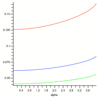
Figure 1: The behavior of the relative phase $\theta$ near the LG point for three different values of $p$. Red corresponds to $p=10$, blue corresponds to $p=20$ and green corresponds to $p=30$.

It is clear from this discussion that the best option for us is to take the number $p$ as high as possible subject to the tadpole cancellation constraints (2.21). This implies that there are no background D3-branes in the system, and we set $p=N_{O3}$. In fact configurations with background D3-branes would not be stable since there would be an attractive force between D3-branes and magnetized D5-branes. Therefore the system will naturally decay to a configuration in which all D3-branes have been converted into magnetic flux on D5-branes.

In order for the above construction to be valid, one has to check whether the D3-brane and D5-brane are stable BPS states at the Landau-Ginzburg point. This is clear in a neighborhood of the large radius limit, but in principle, these BPS states could decay before we reach the Landau-Ginzburg point. For example it is known that in the $\mathbb{C}^{2}/\mathbb{Z}_{3}$ local model the D5-brane decays before we reach the orbifold point in the Kähler moduli space [79]. The behavior of the BPS spectrum of compact Calabi-Yau threefolds is less understood at the present stage. At best one can check stability of a BPS state with respect to a particular decay channel employing $\Pi$-stability techniques [64, 62, 63], but we cannot rigorously prove stability using the formalism developed in [80, 81]. In appendix A we show that magnetized D5-branes on the octic are stable with respect to the most natural decay channels as we approach the Landau-Ginzburg point. This is compelling evidence for their stability in this region of the moduli space, but not a rigorous proof. Based on this amount of evidence, we will assume in the following that these D-branes are stable in a neighborhood of the Landau-Ginzburg point. Our next task is the computation of supergravity D-terms in the mirror IIA orientifold described in section 2.1.

3.2 Mirror Symmetry and Supergravity D-terms

The above $\Pi$-stability arguments are independent of complex structure deformations of the IIB threefold $X$. We can exploit this feature to our advantage by working in a neighborhood of the LCS point in the complex structure moduli space of $X$. In this region, the theory admits an alternative description as a large volume IIA orientifold on the mirror threefold $Y$. The details have been discussed in section 2.1. In the following we will use the IIA description in order to compute the D-term effects on magnetized branes.

Open string mirror symmetry maps the D5-branes wrapping $C,C^{\prime}$ to D6-branes wrapping special lagrangian cycles $M,M^{\prime}$ in $Y$. Since $C,C^{\prime}$ are rigid disjoint $(-1,-1)$ curves for generic moduli of $X$, $M,M^{\prime}$ must be rigid disjoint three-spheres in $Y$. The calibration conditions for $M,M^{\prime}$ are of the form

$${\hbox{Im}}(e^{i\theta}\Omega_{Y}|_{M})=0\qquad{\hbox{Im}}(e^{-i\theta}\Omega_{Y}|_{M^{\prime}})=0.$$ (3.4)

where $\Omega_{Y}$ is normalized so that the calibration of the IIA orientifold O6-planes has phase $1$. The phase $e^{i\theta}$ in (3.4) is equal to the relative phase (3.3) computed above, and depends only on the complex structure moduli of $Y$. The homology classes of these cycles can be read off from the central charge formula (3.2). We have

$$[M]=p\beta^{0}+\beta^{1},\qquad[M^{\prime}]=p\beta^{0}-\beta^{1}$$ (3.5)

where $[M],[M^{\prime}]$ are cohomology classes on $Y$ related to $M,M^{\prime}$ by Poincaré duality.

Taking into account $N=1$ supergravity constraints, the D-term contribution is of the form

$$U_{D}={D^{2}\over 2{\hbox{Im}}(g)}$$ (3.6)

where $g$ is the holomorphic coupling constant of the brane $U(1)$ vector multiplet. The holomorphic coupling constant can be easily determined by identifying the four dimensional axion field $a$ which has a coupling of the form

$$\int aF\wedge F$$ (3.7)

with the $U(1)$ gauge field on the brane. Such couplings are obtained by dimensional reduction of Chern-Simons terms of the form action.

$$\int C^{(3)}\wedge F\wedge F+C^{(5)}\wedge F$$

in the D6-brane world-volume action. Taking into account the expression (2.10) for $C^{(3)}$, dimensional reduction of the Chern-Simons term on the cycle $M$ yields the following four-dimensional couplings

$$p\int\xi^{0}F\wedge F+\int D^{1}\wedge F.$$ (3.8)

Here $\xi^{0}$ is the axion defined in (2.10) and $D^{1}$ is the two-form field obtained by reduction of $C^{(5)}$

$$C^{(5)}=D^{1}\wedge\alpha^{1}.$$

Equation (3.8) shows that the axion field $a$ in (3.7) is $\xi^{0}$. Then, using holomorphy and equation (2.9), it follows that the tree level holomorphic gauge coupling $g$ must be

$$g=2p\tau.$$ (3.9)

The second coupling in (3.8) is also very useful. The two-form field $D^{1}$ is part of an $N=1$ linear multiplet $L^{1}$ whose lowest component is the real field $e^{2\Phi}{\hbox{Im}}(Z^{1})$, where $\Phi$ is the four dimensional dilaton [27]. Moreover, one can relate $L$ to the chiral multiplet $\rho$ by a duality transformation which converts the second term in (3.8) into a coupling of the form

$$\int A_{\mu}\partial^{\mu}{\widetilde{\xi}}_{1}.$$

The supersymmetric completion of this term determines the supergravity D-term to be [82, 83, 84, 85]

$$D=\partial_{\rho}K_{\cal K}.$$ (3.10)

Note that using equation (B.9) in [27], the D-term (3.10) can be written as

$$D=-2e^{2\Phi}{\hbox{Im}}(CZ^{1})$$ (3.11)

where $C$ is the compensator field defined in equation (2.12). Using equations (2.9) and (2.15), we can rewrite (3.11) as

$$D =-2e^{K_{\cal K}/2}{\hbox{Im}}(CZ^{1})$$ (3.12)

$$=-{1\over C}{{\hbox{Im}}(Z^{1})\over{\hbox{Im}}(Z^{1}){\hbox{Re}}(\CF_{1})-{\hbox{Re}}(Z^{0}){\hbox{Im}}(\CF_{0})}$$

$$=-{1\over{\hbox{Im}}(\tau)}{{\hbox{Re}}(Z^{0}){\hbox{Im}}(Z^{1})\over{\hbox{Im}}(Z^{1}){\hbox{Re}}(\CF_{1})-{\hbox{Re}}(Z^{0}){\hbox{Im}}(\CF_{0})}.$$

Then, taking into account (3.9), we find the following expression for the D-term potential energy

$$U_{D}={1\over 4p{\hbox{Im}}(\tau)^{3}}\left[{{\hbox{Re}}(Z^{0}){\hbox{Im}}(Z^{1})\over{\hbox{Im}}(Z^{1}){\hbox{Re}}(\CF_{1})-{\hbox{Re}}(Z^{0}){\hbox{Im}}(\CF_{0})}\right]^{2}.$$ (3.13)

This is our final formula for the D-term potential energy.

In order to conclude this section, we would like to explain the relation between formula (3.13) and the $\Pi$-stability analysis performed earlier in this section. Note that the $\Pi$-stability considerations are captured by an effective potential in the mirror type IIA theory which was found in [76, 77]. According to [76, 77], the D-term potential for a pair of D6-branes as above should be given by

$$V_{D}=2e^{-\Phi}\left(\bigg{|}\int_{M}{\widehat{\Omega}}_{Y}\bigg{|}-\int_{M}{\hbox{Re}}({\widehat{\Omega}}_{Y})\right)$$ (3.14)

where ${\widehat{\Omega}}_{Y}$ is the holomorphic three-form on $Y$ normalized so that

$$i\int_{Y}{\widehat{\Omega}}_{Y}\wedge{\overline{\widehat{\Omega}}_{Y}}=1.$$

Recall that $\Phi$ denotes the four dimensional dilaton.

In the following we would like to explain that this expression is in agreement with the supergravity formula (3.13) for a small supersymmetry breaking angle $|\theta|<<1$. For large $|\theta|$ the effective supergravity description of the theory breaks down, and we would have to employ string field theory in order to obtain reliable results.

Note that one can write

$${\widehat{\Omega}}_{Y}=e^{K_{0}/2}\Omega_{Y}$$ (3.15)

where $K_{0}$ is has been defined in equation (2.13), and $\Omega_{Y}$ has some arbitrary normalization. The expression in the right hand side of this equation is left invariant under rescaling $\Omega_{Y}$ by a nonzero constant.

Formula (3.14) is written in the string frame. In order to compare it with the supergravity expression, we have to rewrite it in the Einstein frame. In the present context, the string metric has to be rescaled by a factor of $e^{2\phi}(\hbox{vol}(Y))^{-1}=e^{2\Phi}$ [86], hence the potential energy in the Einstein frame is

$$V_{D}^{E}=2e^{3\Phi}\left(\bigg{|}\int_{M}{\widehat{\Omega}}_{Y}\bigg{|}-\int_{M}{\hbox{Re}}({\widehat{\Omega}}_{Y})\right).$$ (3.16)

Taking into account equations (3.5) and (3.15) we have

$$\int_{M}{\widehat{\Omega}}_{Y} =e^{K_{0}/2}(p{\hbox{Re}}(Z^{0})+i{\hbox{Im}}(Z^{1}))=e^{K_{0}/2}Z_{+}$$

where $Z_{+}$ is the central charge defined in equation (3.1). For small values of the phase, $|\theta|<<1$, we can expand (3.16) as

$$V_{D}^{E}\sim e^{3\Phi}e^{K_{0}/2}{{\hbox{Re}}(Z_{0})\over p}\left[{{\hbox{Im}}(Z^{1})\over{\hbox{Re}}(Z^{0})}\right]^{2}.$$ (3.17)

Now, using equations (2.9) and (3.11) in (3.6), we obtain

$$U_{D} =Ce^{4\Phi}{{\hbox{Re}}(Z^{0})\over p}\left[{{\hbox{Im}}(Z^{1})\over{\hbox{Re}}(Z^{0})}\right]^{2}=e^{3\Phi}e^{K_{0}/2}{{\hbox{Re}}(Z^{0})\over p}\left[{{\hbox{Im}}(Z^{1})\over{\hbox{Re}}(Z^{0})}\right]^{2}$$ (3.18)

Therefore the supergravity D-term potential agrees indeed with (3.14) for very small supersymmetry breaking angle. This generalizes the familiar connection between $\Pi$-stability and D-term effects to supergravity theories. In order to complete the description of the dynamics, we will focus next on superpotential interactions.

4 Fluxes, Branes and Superpotential Interactions

In this section we study superpotential interactions of magnetized branes in Calabi-Yau orientifolds with background fluxes. Brane-flux superpotentials have been first discussed in [39, 40]. Our treatment is based on the same idea, although our treatment of compact Calabi-Yau situations will be closer to [41, 42].

Let us first consider magnetized branes in the absence of fluxes. The fluxes will naturally enter the picture at a later stage. Our first task is to identify the lowest lying modes which govern the low energy physics in the presence of D-branes. The massless fields correspond to marginal deformations of the internal bulk-boundary CFT. Suppose we have a D-brane wrapping a holomorphic curve $C$ in a Calabi-Yau threefold $X$. The marginal deformations of the bulk-boundary CFT are in one-to-one correspondence with deformations of the pair $(X,C)$. The infinitesimal deformations of $X$ are classified by $H^{1}(X,T_{X})$. Using a standard spectral sequence, one can show that the space ${\mathbb{H}}$ of infinitesimal deformations of the pair $(X,C)$ fits in an exact sequence the form

(4.1)

where $N_{C/X}$ is the normal bundle to $C$ in $X$. The map $f:H^{1}(X,T_{X})\to H^{1}(C,N_{C/X})$ is induced by the natural projection $T_{X}\to N_{C/X}$.

From a physical point of view the first term in (4.1), $H^{0}(C,N_{C/X})$ parameterizes marginal boundary operators. The third term $H^{1}(X,T_{X})$ parameterizes marginal deformations of the bulk CFT in the absence of boundaries. It is important to note that not all these marginal operators remain marginal in the bulk-boundary CFT. In fact the exact sequence (4.1) shows that only those deformations in $H^{1}(X,T_{X})$ which map to zero in $H^{1}(C,N_{C/X})$ are marginal deformations of the bulk-boundary theory.

In our case the Calabi-Yau threefold $X$ is equipped with a holomorphic involution $\sigma$, and and the magnetized branes are wrapped on two disjoint curves $C,C^{\prime}=\sigma(C)$ on $X$. Then the infinitesimal deformations are captured by the invariant part of (4.1) with respect to $\sigma$

(4.2)

Let us denote by $\CN$ a connected component of the moduli space of data $(X,\sigma,C,C^{\prime})$. Note that there is a natural forgetful map $\rho:\CN\to\CM$, where $\CM$ is a connected component of the moduli space of Calabi-Yau threefolds $(X,\sigma)$ with involution. At a generic point in $\CN$, $C,C^{\prime}$ are $(-1,-1)$ curves on $X$, hence

$$H^{0}(C,N_{C/X})=H^{0}(C^{\prime},N_{C^{\prime}/X})=0.$$

The only low energy light modes near such a point in the moduli space correspond to deformations of $X$ which preserve $(\sigma,C,C^{\prime})$. The map $\rho:\CN\to\CM$ is locally finite-to-one near such a point. However, the curves $C,C^{\prime}$ may have nontrivial normal deformations in $X$ for special values of the complex structure moduli. These normal deformations yield new light fields which have to be taken into account in the low energy effective action. This behavior is similar in spirit with the Seiberg-Witten solution of $N=2$ gauge theories. Around each point, the low energy theory will have an effective superpotential which is a holomorphic function of the lightest fields in the spectrum near that point.

The local expression of the superpotential on $\CN$ is given by a three-chain period of the holomorphic three-form on $X$ [37, 38]. More precisely, the space $\CN$ can be locally identified near each point $(X,\sigma,C,C^{\prime})$ with an open set $\CU$ in the linear space

$$H^{0}(C,N_{C/X})\oplus\hbox{Ker}(f_{+}).$$

Let us pick a three chain $\Gamma_{0}$ interpolating between $C,C^{\prime}$ on $X$ i.e.

$$\partial\Gamma=C^{\prime}-C.$$

Then we can extend $\Gamma_{0}$ to a multivalued family of three-chains $\Gamma_{u}$, $u\in\CU$ so that

$$\partial\Gamma_{u}=C_{u}-C^{\prime}_{u}$$

for each $u\in\CU$ [41]. This extension is obtained by transporting the three-chain $\Gamma_{0}$ to any point in $\CU$ using the Gauss-Manin connection. The superpotential is a holomorphic function on $\CU$ given by

$$W=\int_{\Gamma_{u}}\Omega_{X_{u}}$$ (4.3)

where $\Omega_{X_{u}}$ is the global holomorphic three-form on $X_{u}$. Since the overall normalization of $\Omega_{X_{u}}$ is not fixed, (4.3) actually defines a local section of the line bundle $\rho^{*}\CL$ over $\CU$.

Note that the expression (4.3) is ambiguous since the chain $\Gamma_{0}$ is only defined up to a shift

$$\Gamma_{0}\to\Gamma_{0}+\gamma.$$ (4.4)

where $\gamma$ is a closed three-cycle on $X$. This is not a problem from a mathematical point of view since one can show that the critical set of $W$ is independent of the choice of $\Gamma_{0}$. Nevertheless this ambiguity has a very natural physical interpretation because we can interpret a shift of the form (4.4) as a shift in the background RR flux. More precisely, note that the shift (4.4) changes the superpotential (4.3) by

$$\Delta W=\int_{\gamma_{u}}\Omega_{X_{u}}$$

where $\gamma_{u}$ is again a family of three-cycles obtained by parallel transport with respect to the Gauss-Manin connection. Therefore, using Poincaré duality, we can identify the ambiguity in the choice of $\Gamma_{0}$ with a shift

$$F\to F+\eta$$

in the background RR flux $F$ on $X$, where $\eta\in H^{3}(X,\mathbb{Z})$ is the Poincaré dual of $\gamma$. This identification is natural since in the presence of D-branes, the RR flux is not well defined as an element of $H^{3}(X,\mathbb{Z})$; an element of $H^{3}(X,\mathbb{Z})$ only determines a shift in the background flux, but the overall value of the flux depends on the choice of a trivialization of the D-brane charge [87]. More formally, the RR fluxes take values in a torsor over $H_{3}(X,\mathbb{Z})$.

We are therefore led to the conclusion that in superstring compactifications, the superpotential (4.3) should be interpreted as a combined brane – RR flux superpotential. There is no natural way of splitting this formula in separate brane and respectively RR flux contributions, but changes in the background flux are captured by shifts of the form (4.4). Although in this section we have used IIB variables, (4.3) can be equally interpreted as a IIA superpotential using open string mirror symmetry.

We conclude this discussion with a few remarks. In the next section we will investigate the vacuum structure of magnetized branes in the octic orientifold taking into account both F-term and D-term effects.

$(i)$ The superpotential (4.3) depends only on the complex structure deformations of $X$ which preserve the curve $C$. In general these deformations span a proper closed subspace of the moduli space $\CM$. We argued that the remaining complex moduli of $X$ are generically massive and do not appear in the low energy effective action. This argument is in principle correct at generic points in the moduli space, but it may fail at special points in the moduli space where the fields we have integrated out become light. Such effects can be taken into account extending the superpotential (4.3) to a local function of all complex structure moduli. Let us consider an open subset ${\mathcal{V}}$ of

$$H^{0}(C,N_{C/X})\oplus H^{1}(X,T_{X})$$

containing $\CU$ as a closed subset. Then we can use the Gauss-Manin connection to extend the three-chain $\Gamma_{0}$ to a family of three-chains $\Gamma_{v}$ labeled by points in ${\mathcal{V}}$ and define the extension of $W$ to be

$$W=\int_{\Gamma_{v}}\Omega_{X_{v}}.$$ (4.5)

The main difference with respect to the previous case is that the boundary of $\Gamma_{v}$ is no longer a holomorphic cycle on $X_{v}$ if $v$ is not in $\CU$.

$(ii)$ The low energy theory may contain extra light open string fields at points in the moduli space $\CN$ where the two curves $C,C^{\prime}$ coincide. Then we will have additional superpotential interactions involving these fields as well.

$(iii)$ The expression (4.3) is very similar to the flux superpotential (2.19). In particular they have the same tree level dependence on the dilaton multiplet $\tau$ and they are subject to the same axion shift symmetries. Therefore, using the same low energy arguments as [60] one can show that (4.3) is subject to the same nonrenormalization result. This means that this formula is reliable at small IIB volume.

$(iv)$ In general situations, the superpotential (4.3) cannot be canonically split into a brane contribution and a flux contribution of the form (2.19). However, in special cases, this is possible using specific features of the geometry. For example suppose the threefold $X$ contains a connected family of holomorphic curves interpolating between $C,C^{\prime}$. Then one can choose the three-chain $\Gamma$ to be swept by a real one-parameter family of holomorphic curves in $X$. It is known that the period of $\Omega_{X}$ on such three-chains vanishes. Therefore if we make such a choice, the superpotential (4.3) will be identically zero. Then a shift of the form (4.4) will produce a superpotential of the form (2.19).

5 The D-Brane Landscape

In this section we explore the magnetized D-brane landscape in the octic orientifold model introduced in section 2. We compute the F-term and D-term contributions in a neighborhood of the Landau-Ginzburg point in the IIA complex structure moduli space ${\cal K}$. For technical reasons we will not be able to find explicit solutions to the critical point equations. However, given the shape of the potential, we will argue that metastable vacuum solutions are statistically possible by tuning the values of fluxes.

Throughout this section we will be working at a generic point in the configuration space where all open string fields are massive and can be integrated out. Following the reasoning of the previous section, this is the expected behavior for D-branes wrapping isolated rigid holomorphic curves in a Calabi-Yau threefold. One should however be aware of several possible loopholes in this assumption since open string fields may become light along special loci in the moduli space.

In our situation, one should be especially careful with the open string-fields in the brane anti-brane sector. According to the $\Pi$-stability analysis in section 3, there is a tachyonic contribution to the mass of the lightest open string modes proportional to the phase difference $\theta$. At the same time, we have a positive contribution to the mass due to the tension of the string stretching between the branes. In order to avoid tachyonic instabilities, we should work in a region of the moduli space where the positive contribution is dominant. Since the curves are isolated, the positive mass contribution is generically of the order of the string scale, which is much larger than the tachyonic contribution, since $\theta$ is of the order $0.05$. Therefore we do not expect tachyonic instabilities in the system as long as the moduli are sufficiently generic.

This argument can be made more precise in the mirror IIA picture. As discussed in section 3.2, the IIA description of the system involves two disjoint special lagrangian cycles $M,M^{\prime}$ on the Calabi-Yau manifold $Y$. The position of $M,M^{\prime}$ in $Y$ is determined by the calibration conditions (3.4), which are invariant under a rescaling of the metric on $Y$ by a constant $\lambda>1$. Such a rescaling would also increase the minimal geodesic distance between $Y,Y^{\prime}$, which determines the mass of the open string modes. Therefore, if the volume of $Y$ is sufficiently large, we expect the brane anti-brane fields to have masses at least of the order of the string scale.

Even if the open string fields have a positive mass, the system can still be destabilized by the brane anti-brane attraction force. Generically, we expect this not to be the case as long as the brane-brane fields are sufficiently massive since the attraction force is proportional to $\theta$ and it is also suppressed by a power of the string coupling. We can understand the qualitative aspects of the dynamics using a simplified model for the potential energy. Suppose that the effective dynamics of the branes can be described in terms of a single light chiral superfield $\Phi$. Typically this happens when we work near a special point $X_{0}$ in the complex structure moduli space where the curves $C,C^{\prime}$ belong to a one parameter family $\CC$ of holomorphic curves. The field $\Phi$ corresponds to normal deformations of the brane wrapping $C$, which are identified with normal deformations of the anti-brane wrapping $C^{\prime}$ by the orientifold projection. A sufficiently generic small complex deformation of $X$ away from $X_{0}$ induces a mass term for $\Phi$. Therefore we can model the effective dynamics of the system by a potential of the form

$$m(r-r_{0})^{2}+c\ln\left({r\over r_{0}}\right)$$

where $r$ parameterizes the separation between the branes. The quadratic terms models a mass term for the open string fields corresponding to normal deformations of the branes in the ambient manifold. The second term models a typical two dimensional attractive brane anti-brane potential. The constant $c>0$ is proportional to the phase $\theta$ and the string coupling $g_{s}$. Now one can check that if $c<<mr_{0}$, this potential has a local minimum near $r=r_{0}$, and the local shape of the potential near this minimum is approximatively quadratic. In our case, we expect $m,r_{0}$ to be typically of the order of the string scale, whereas $c\sim g_{s}\theta\sim 10^{-2}$ therefore the effect of the attractive force is negligible.

Since it is technically impossible to make these arguments very precise, we will simply assume that there is a region in configuration space where destabilizing effects are small and do not change the qualitative behavior of the system. Moreover, all open string fields are massive, and we can describe the dynamics only in terms of closed string fields. This point of view suffices for a statistical interpretation of the D-brane landscape. By tuning the values of fluxes, one can in principle explore all regions of the configuration space. The vacuum solutions which land outside the region of validity of this approximation will be automatically destabilized by some of these effects. Therefore there is a natural selection mechanism which keeps only vacuum solutions located at a sufficiently generic point in the moduli space.

Granting this assumption, we will take the configuration space to be isomorphic to the closed string moduli space $\CM\times{\cal K}$ described in section 2.1. As discussed in section 2.2, we will turn on only RR fluxes $F^{A}=F_{2}+F_{4}+F_{6}$ and NS-NS flux $H^{A}$. In the presence of branes, the NS-NS flux $H^{A}$ must satisfy the Freed-Witten anomaly cancellation condition [88], which states that the the restriction of $H^{A}$ to the brane world-volumes $M,M^{\prime}$ must be cohomologically trivial. Taking into account equations (2.17), (3.5), it follows that the integer $q_{1}$ in (2.17) must be set to zero. Therefore the superpotential does not depend on the chiral superfield $\rho$. This can also be seen from the analysis of supergravity D-terms in section 3.2. The $U(1)$ gauge group acts as an axionic shift symmetry on $\rho$, therefore gauge invariance rules out any $\rho$-dependent terms in the superpotential [89]. The connection between the Freed-Witten anomaly condition and supergravity has been observed before in [31].

The total effective superpotential is then given by

$$W=\int_{\Gamma}\Omega_{X}-2p^{0}\tau,$$ (5.1)

where $\Gamma$ is a three-chain on $X$ interpolating between the two curves $C,C^{\prime}$. As explained in remark (i) section 4, this expression makes sense over the entire moduli space $\CM$ although some complex structure deformations may not preserve the curves $C,C^{\prime}$. This only means that some complex structure moduli fields are actually massive, and their mass terms are encoded in $W$. Alternatively, one can take the configuration space to be of the form $\CN\times{\cal K}$ by integrating out the massive fields, but the two points of view are equivalent, at least generically.

The F-term contribution to the potential energy is

$$U_{F}=e^{K}\left(g^{i{\bar{\jmath}}}(D_{i}W)(D_{\bar{\jmath}}{\overline{W}})+g^{a{\bar{b}}}(D_{a}W)(D_{\bar{b}}{\overline{W}})-3|W|^{2}\right).$$ (5.2)

where $i,j,\ldots$ label complex coordinates on $\CM$ and and $a,b=\rho,\tau$ label complex coordinates on ${\cal K}$. The D-term contribution is given by equation (3.13). We reproduce it below for convenience

$$U_{D}={1\over 4p{\hbox{Im}}(\tau)^{3}}\left[{{\hbox{Re}}(Z^{0}){\hbox{Im}}(Z^{1})\over{\hbox{Im}}(Z^{1}){\hbox{Re}}(\CF_{1})-{\hbox{Re}}(Z^{0}){\hbox{Im}}(\CF_{0})}\right]^{2}.$$

Since the moduli space of the theory is a direct product ${\cal K}\times\CM$, the Kähler potential $K$ in (5.2) is

$$K=K_{\cal K}+K_{\CM}.$$

Note that we Kähler potentials $K_{{\cal K}}$, $K_{\CM}$ satisfy the following noscale relations [27]

$$g^{i{\bar{j}}}\partial_{i}K_{\CM}\partial_{\bar{j}}K_{\CM}=3\qquad g^{a{\bar{b}}}\partial_{a}K_{\cal K}\partial_{\bar{b}}K_{\cal K}=4.$$ (5.3)

Using equations (2.9) and (2.14), we have

$$e^{K_{{\cal K}}}={1\over 4{\hbox{Im}}(\tau)^{4}}\left[{{\hbox{Re}}(Z^{0})^{2}\over{\hbox{Im}}(Z^{1}){\hbox{Re}}(\CF_{1})-{\hbox{Re}}(Z^{0}){\hbox{Im}}(\CF_{0})}\right]^{2}.$$

Now we have a complete description of the potential energy of the system. Finding explicit vacuum solutions using these equations seems to be a daunting computational task, given the complexity of the problem. We can however gain some qualitative understanding of the resulting landscape by analyzing the potential energy in more detail.

First we have to find a convenient coordinate system on the moduli space ${\cal K}$. Note that the potential energy is an implicit function of the holomorphic coordinates $(\tau,\rho)$ via relations (2.9). One could expand it as a power series in $(\tau,\rho)$, but this would be an awkward process. Moreover, the axion ${\widetilde{\xi}}_{1}={\hbox{Im}}(\rho)$ is eaten by the $U(1)$ gauge field, and does not enter the expression for the potential. Therefore it is more natural to work in coordinates $(\tau,\alpha)$ where $\alpha$ is the algebraic coordinate on the underlying $N=2$ Kähler moduli space. As explained in section 2.1, $\alpha$ takes real values in the orientifold theory.

There is a more conceptual reason in favor of the coordinate $\alpha$ instead of $\rho$, namely $\alpha$ is a coordinate on the Teichmüller space of $Y$ rather than the complex structure moduli space. Since in the $\Pi$-stability framework the phase of the central charge is defined on the Teichmüller space, $\alpha$ is the natural coordinate when D-branes are present.

Next, we expand the potential energy in terms of $(\tau,\alpha)$ using the relations (2.9). Dividing the two equations in (2.9), we obtain

$${\rho+{\overline{\rho}}\over\tau-{\overline{\tau}}}=2i{{\hbox{Re}}(\CF_{1})\over{\hbox{Re}}(Z^{0})}$$ (5.4)

Let us denote the ratio of periods in the right hand side of equation (2.9) by

$$R(\alpha)={{\hbox{Re}}(\CF_{1})\over{\hbox{Re}}(Z^{0})}.$$ (5.5)

Using equations (5.4) and (5.5), we find the following relations

$${\partial\alpha\over\partial\rho}={1\over 2i}{1\over\tau-{\overline{\tau}}}\left({\partial R\over\partial\alpha}\right)^{-1}\qquad{\partial\alpha\over\partial\tau}=-{R\over\tau-{\overline{\tau}}}\left({\partial R\over\partial\alpha}\right)^{-1}.$$ (5.6)

Now, using the chain differentiation rule, we can compute the derivatives of the Kähler potential as functions of $(\tau,\alpha)$. Let us introduce the notation

$$V(\alpha)={{\hbox{Im}}(Z^{1}){\hbox{Re}}(\CF_{1})-{\hbox{Re}}(Z^{0}){\hbox{Im}}(\CF_{0})\over{\hbox{Re}}(Z^{0})^{2}}.$$

Then we have

$$\partial_{\tau}K_{\cal K} =-\partial_{\bar{\tau}}K_{\cal K}=-{2\over\tau-{\overline{\tau}}}\left[2-R{\partial_{\alpha}V\over V}\left({\partial_{\alpha}R}\right)^{-1}\right]$$ (5.7)

$$\partial_{\rho}K_{\cal K} =\partial_{\bar{\rho}}K_{\cal K}={i\over\tau-{\overline{\tau}}}{\partial_{\alpha}V\over V}\left({\partial_{\alpha}R}\right)^{-1}$$

$$\partial_{\tau{\bar{\tau}}}K_{\cal K} =-{2\over(\tau-{\overline{\tau}})^{2}}\left[2-R{\partial_{\alpha}V\over V}\left({\partial_{\alpha}R}\right)^{-1}-R\partial_{\alpha}\left(R{\partial_{\alpha}V\over V}(\partial_{\alpha}R)^{-1}\right)(\partial_{\alpha}R)^{-1}\right]$$

$$\partial_{\tau{\bar{\rho}}}K_{\cal K} =-\partial_{\rho{\bar{\tau}}}K_{\cal K}=-{i\over(\tau-{\overline{\tau}})^{2}}\left[{\partial_{\alpha}V\over V}\left({\partial_{\alpha}R}\right)^{-1}+R\partial_{\alpha}\left({\partial_{\alpha}V\over V}(\partial_{\alpha}R)^{-1}\right)(\partial_{\alpha}R)^{-1}\right]$$

$$\partial_{\rho{\bar{\rho}}}K_{\cal K} ={1\over 2(\tau-{\overline{\tau}})^{2}}\partial_{\alpha}\left({\partial_{\alpha}V\over V}(\partial_{\alpha}R)^{-1}\right)(\partial_{\alpha}R)^{-1}$$

Using equations (5.7), and the power series expansions of the periods computed in appendix A, we can now compute the expansion of the potential energy as in terms of $(\tau,\alpha)$. The D-term contribution takes the form

$$U_{D}={1\over p{\hbox{Im}}(\tau)^{3}}(0.03125-0.00178\alpha^{2}+0.00005\alpha^{4}+\ldots).$$ (5.8)

We will split the F-term contribution into two parts

$$U_{F}=U_{F}^{\CM}+U_{F}^{{\cal K}}$$

where

$$U_{F}^{\CM} =e^{K_{\cal K}+K_{\CM}}\left(g^{i{\bar{\jmath}}}(D_{i}W)(D_{\bar{\jmath}}{\overline{W}})-3|W|^{2}\right)$$

$$U_{F}^{\cal K} =e^{K_{\cal K}+K_{\CM}}\left(g^{a{\bar{b}}}(D_{a}W)(D_{\bar{b}}{\overline{W}})\right).$$

We will also write the superpotential (5.1) in the form

$$W=W_{0}(z^{i})+k\tau$$

where $k=-2p^{0}$. The factor $e^{K_{\cal K}}$ and the inverse metric coefficients $g^{a{\bar{b}}}$ can be expanded in powers of $\alpha$ using the equations (5.7) and formulas (A.5) in appendix A. Using the noscale relations (5.3), we find the following expressions

$$U_{F}^{\CM}={e^{K_{\CM}}\over 4{\hbox{Im}}(\tau)^{4}}(0.0625-0.00357\alpha^{2}+0.00004\alpha^{4}+\ldots)$$ (5.9)

$$\left(g^{i{\bar{\jmath}}}(\partial_{i}W_{0})(\partial_{\bar{\jmath}}{\overline{W}}_{0})+g^{i{\bar{\jmath}}}[(\partial_{i}W_{0})(\partial_{\bar{\jmath}}K_{\CM})({\overline{W}}_{0}+k{\overline{\tau}})+(\partial_{\bar{\jmath}}{\overline{W}}_{0})(\partial_{i}K_{\CM})(W_{0}+k\tau)]\right)$$

$$U_{F}^{{\cal K}}= {e^{K_{\CM}}\over{\hbox{Im}}(\tau)^{4}}\bigg{[}{\hbox{Im}}(\tau)^{2}(0.03125-0.00073\alpha^{2}+0.00001\alpha^{4}+\ldots)k^{2}$$ (5.10)

$$-{\hbox{Im}}(\tau)(0.03125-0.00178\alpha^{2}+0.00002\alpha^{4}+\ldots)(2k^{2}{\hbox{Im}}(\tau)+2k{\hbox{Im}}(W_{0}))$$

$$+(0.0625-0.00357\alpha^{2}+0.00004\alpha^{4}+\ldots)(k^{2}\tau{\overline{\tau}}+k\tau{\overline{W}_{0}}+k{\overline{\tau}}W_{0}+|W_{0}|^{2})\bigg{]}$$

Let us now try to analyze the shape of the landscape determined by the equations (5.8) and (5.9), (5.10). We rewrite the contribution (5.9) to the potential energy in the form

$$U_{F}^{\CM}={e^{K_{\CM}}\over 4{\hbox{Im}}(\tau)^{4}}(0.0625-0.00357\alpha^{2}+0.00004\alpha^{4}+\ldots)\left(P+kM{\hbox{Re}}(\tau)+kN{\hbox{Im}}(\tau)\right)$$ (5.11)

where

$$P=g^{i{\bar{\jmath}}}(\partial_{i}W_{0})(\partial_{\bar{\jmath}}{\overline{W}}_{0})+g^{i{\bar{\jmath}}}[(\partial_{i}W_{0})(\partial_{\bar{\jmath}}K_{\CM}){\overline{W}}_{0}+(\partial_{\bar{\jmath}}{\overline{W}}_{0})(\partial_{i}K_{\CM})W_{0}]$$ (5.12)

$$M=g^{i{\bar{\jmath}}}[(\partial_{i}W_{0})(\partial_{\bar{\jmath}}K_{\CM})+(\partial_{\bar{\jmath}}{\overline{W}}_{0})(\partial_{i}K_{\CM})]$$

$$N=(-i)g^{i{\bar{\jmath}}}[(\partial_{i}W_{0})(\partial_{\bar{\jmath}}K_{\CM})-(\partial_{\bar{\jmath}}{\overline{W}}_{0})(\partial_{i}K_{\CM})]$$

Then the $\alpha$ expansion of the F-term potential energy can be written as

$$U_{F}=U_{F}^{(0)}+\alpha^{2}U_{F}^{(2)}+\ldots$$

where

$$U_{F}^{(0)}=0.0156{e^{K_{\CM}}\over{\hbox{Im}}(\tau)^{4}}[ P+k(N+4{\hbox{Im}}(W_{0})){\hbox{Im}}(\tau)+2k^{2}{\hbox{Im}}(\tau)^{2}$$ (5.13)

$$+4|W_{0}|^{2}+k(M+8{\hbox{Re}}(W_{0})){\hbox{Re}}(\tau)+4k^{2}{\hbox{Re}}(\tau)^{2}]$$

$$U_{F}^{(2)}=-0.00178{e^{K_{\CM}}\over 2{\hbox{Im}}(\tau)^{4}}[ P+k(N+4{\hbox{Im}}(W_{0})){\hbox{Im}}(\tau)+0.82k^{2}{\hbox{Im}}(\tau)^{2}$$ (5.14)

$$+4|W_{0}|^{2}+k(M+8{\hbox{Re}}(W_{0})){\hbox{Re}}(\tau)+4k^{2}{\hbox{Re}}(\tau)^{2}]$$

The critical point equations resulting from (5.8), (5.9) and (5.10) are very complicated, and we will not attempt to find explicit solutions. We will try to gain some qualitative understanding of the possible solutions exploiting some peculiar aspects of the potential. Note that all contributions to the potential energy depend on even powers of $\alpha$. Then it is obvious that $\alpha=0$ is a solution to the equation

$$\partial_{\alpha}U=0$$

where $U=U_{D}+U_{F}^{\CM}+U_{F}^{\cal K}$. Moreover we also have

$$(\partial_{i}\partial_{\alpha}U)_{\alpha=0}=(\partial_{\tau}\partial_{\alpha}U)_{\alpha=0}=0.$$

This motivates us to look for critical points with $\alpha=0$. Then, the remaining critical point equations are

$$(\partial_{i}U)_{\alpha=0}=(\partial_{\tau}U)_{\alpha=0}=0$$ (5.15)

plus their complex conjugates.

The second order coefficient of $\alpha$ in the total potential energy is

$$U_{F}^{(2)}-0.00178{1\over p{\hbox{Im}}(\tau)^{3}}.$$ (5.16)

Since the mixed partial derivatives are zero at $\alpha=0$, in order to obtain a local minimum, the expression (5.16) must be positive. This is a first constraint on the allowed solutions to (5.15).

Next, let us examine the $\tau$ dependence of the potential for $\alpha=0$ and fixed values of the Kähler parameters. Note that $U_{F}^{(0)}$ given by equation (5.13) is a quadratic function of the axion ${\hbox{Re}}(\tau)$. For any fixed values of ${\hbox{Im}}(\tau)$ and the Kähler parameters, this function has a minimum at

$${\hbox{Re}}(\tau)=-{8{\hbox{Re}}(W_{0})+M\over 8k}.$$ (5.17)

Therefore we can set ${\hbox{Re}}(\tau)$ to its minimum value in the potential energy, obtaining an effective potential for the Kähler parameters and the dilaton ${\hbox{Im}}(\tau)$. Then equations (5.13), (5.14) become

$$U_{F}^{(0)}=0.0156{e^{K_{\CM}}\over{\hbox{Im}}(\tau)^{4}}\bigg{[} P+k(N+4{\hbox{Im}}(W_{0})){\hbox{Im}}(\tau)+2k^{2}{\hbox{Im}}(\tau)^{2}$$ (5.18)

$$+4|W_{0}|^{2}-{1\over 16}(M+8{\hbox{Re}}(W_{0}))^{2}\bigg{]}$$

$$U_{F}^{(2)}=-0.00178{e^{K_{\CM}}\over 2{\hbox{Im}}(\tau)^{4}}\bigg{[} P+k(N+4{\hbox{Im}}(W_{0})){\hbox{Im}}(\tau)+0.82k^{2}{\hbox{Im}}(\tau)^{2}$$ (5.19)

$$+4|W_{0}|^{2}-{1\over 16}(M+8{\hbox{Re}}(W_{0}))^{2}\bigg{]}$$

Now let us analyze the dependence of $U_{F}^{(0)}$ on ${\hbox{Im}}(\tau)$. It will be more convenient to make the change of variables

$$u={1\over{\hbox{Im}}(\tau)}$$

since $u$ is proportional to the string coupling constant. Then $U_{F}^{(0)}$ becomes a quartic function of the form

$$U_{F}^{(0)}=Au^{2}-Bu^{3}+Cu^{4}$$ (5.20)

where

$$A=2k^{2}$$ (5.21)

$$B=-kN-4k{\hbox{Im}}(W_{0})$$

$$C=P+4|W_{0}|^{2}-{1\over 16}(M+8{\hbox{Re}}(W_{0}))^{2}.$$

The behavior of this function for fixed values of the Kähler parameters is very simple. For positive $A$, this function has a local minimum away from the origin if and only if the following inequalities are satisfied

$$B>0\qquad C>0\qquad\hbox{and}\qquad 9B^{2}>32AC.$$ (5.22)

The minimum is located at

$$u_{0}={3B+\sqrt{9B^{2}-32AC}\over 8C}.$$ (5.23)

Therefore, in order to construct metastable vacua, we have to find solutions to the equations (5.15) satisfying the inequalities (5.22). Moreover, we would like $u_{0}$ to be small in order to obtain a weakly coupled theory. The conditions (5.22) translate to

$$9(N+4{\hbox{Im}}(W_{0}))^{2} >64\left(P+4{\hbox{Im}}(W_{0})^{2}-M{\hbox{Re}}(W_{0})-{M^{2}\over 16}\right)>0$$ (5.24)

$$k\left(N+{\hbox{Im}}(W_{0})\right)<0$$

where $P,M,N$ are given by (5.12). This shows that we need a certain amount of fine tuning of the background RR fluxes in order to obtain a metastable vacuum. Note that in our construction the fluxes are not constrained by tadpole cancellation conditions, therefore we can tune them at will. Statistically, this improves our chances of finding a solution with the required properties.

Finally, note that we have to impose one more condition, namely the second order coefficient (5.16) in the $\alpha$ expansion of the potential should be positive. Assuming that we have found a solution of equations (5.15) which stabilizes $u$ at the value $0<u_{0}<1$, let us compute this coefficient as a function of $(u_{0},A,B,C)$. Note that equation (5.19) can be rewritten as

$$U_{F}^{(2)}=0.00178{e^{K_{\CM}}\over 2}(Bu_{0}^{3}-0.4Au_{0}^{2}-Cu_{0}^{4}).$$ (5.25)

Equation (5.23) yields

$$B={4\over 3}Cu_{0}+{2\over 3}{A\over u_{0}}$$ (5.26)

Substituting (5.26) in (5.25), and adding the D-term contribution, the coefficient of $\alpha^{2}$ becomes

$$0.00178\left[{e^{K_{\CM}}}({2\over 15}Au_{0}^{2}+{1\over 6}Cu_{0}^{4})-{1\over p}u_{0}^{3}\right]$$ (5.27)

Since $C>0$, a sufficient condition for (5.27) to be positive is

$${2p\over 15}Ae^{K_{\CM}}>u_{0}\quad\Rightarrow\quad{4pk^{2}\over 15}>u_{0}\hbox{vol}(Y).$$ (5.28)

Here we have used

$$e^{K_{\CM}}={1\over\hbox{vol}(Y)}.$$

This condition reflects the fact that the F-term and D-term contributions to the potential energy must be of the same order of magnitude in order to obtain a metastable vacuum solution. If the volume of $Y$ is too large, there is a clear hierarchy of scales between the two contributions, and the D-term is dominant. This would give rise to a runaway behavior along the direction of $\alpha$. On the other hand, we have to make sure that the volume of $Y$ is sufficiently large so that the IIA supergravity approximation is valid. Therefore some additional amount of fine tuning is required in order to obtain a reliable solution.

In conclusion, metastable nonsupersymmetric vacua at $\alpha=0$ can be in principle obtained by tuning the IIA RR flux $F^{(A)}$ and NS-NS flux $H^{A}=k\beta^{0}$ so that conditions (5.24), (5.28) are satisfied at the critical point. A more precise statement would require a detailed numerical analysis, which we leave for future work.

We would like to conclude this section with a few remarks.

$(i)$ In this paper we have taken a conservative approach towards fluxes, avoiding half flat structures in the IIA theory, which correspond to IIB NS-NS flux $H^{B}$. If one is willing to consider compactifications of this form, we have additional terms in the superpotential. In IIB variables, these terms would read

$$-\tau\int_{X}\Omega_{X}\wedge H^{B}.$$

One can also turn on additional flux degrees of freedom as advocated in [90, 91]. Such terms may be helpful in the above fine tuning process.

$(ii)$ We have also restricted ourselves to singly wrapped magnetized D5-branes. One could in principle consider multiply wrapped D5-branes as long we can maintain the phase difference $\theta$ sufficiently small. If this is possible, we would obtain an additional nonperturbative contribution to the superpotential of the form

$$be^{-a\tau}.$$

Such terms may be also helpful in the fine tuning process.

$(iii)$ Finally, note that we could also allow for a nonzero background value of the RR zero-form $F_{0}$, which was also set to zero in this paper. Then, according to [33], there is an additional contribution to the RR tadpole cancellation condition, which becomes

$$p-km_{0}-|N_{O3}|=0.$$

If we choose $k,m_{0}$ so that $km_{0}>0$, it follows that $p$ can be larger than $|N_{O3}|$. In fact it seems that there is no upper bound on $p$, hence we could make the supersymmetry breaking D-term very small by choosing a large $p$. This may have important consequences for the scale of supersymmetry breaking in string theory.

$(iv)$ Note that the vacuum construction mechanism proposed above can give rise to de Sitter or anti de Sitter vacua, depending on the values of fluxes. In particular, it is not subject to the no-go theorem of [92] because the magnetized branes give a positive contribution to the potential energy. In principle we could try to employ the same strategy in order to construct nonsupersymmetric metastable vacua of the F-term potential energy (5.2) in the absence of magnetized branes. Then we have several options for RR tadpole cancellation. We can turn on background $F_{0}$ flux as in [33] or local tadpole cancellation by adding background D6-branes. It would be interesting to explore these alternative constructions in more detail.

$(v)$ Since it is quite difficult to find explicit vacuum solutions, it would be very interesting to attempt a systematic statistical analysis of the distribution of vacua along the lines of [93, 94, 95, 96, 97, 98, 99].

$(vi)$ In our approach the scale of supersymmetry breaking is essentially determined by the total RR tadpole $p=|N_{O3}|$ of the orientifold model. While this tadpole is typically of the order of $32$ in perturbative models, it can reach much higher values in orientifold limits of F-theory. It would be very interesting to implement our mechanism in such an F-theory compactification, perhaps in conjunction with other moduli stabilization mechanism [100, 43, 101, 102, 103, 104, 105]. Provided that the dynamics can still be kept under control, we would then obtain smaller supersymmetry breaking scales.

Appendix A $\Pi$-Stability on the Octic and $N=2$ Kähler Moduli Space

In this appendix we analyze the $N=2$ Kähler moduli space and stability of magnetized branes for the octic hypersurface. Recall [55] that the mirror family is described by the equation

$$x_{1}^{8}+x_{2}^{8}+x_{3}^{8}+x_{4}^{8}+x_{5}^{2}-\alpha x_{1}x_{2}x_{3}x_{4}x_{5}=0.$$ (A.1)

in $WP^{1,1,1,1,4}/(\mathbb{Z}_{8}^{2}\times\mathbb{Z}_{2})$. The moduli space of the mirror family can be identified with a sector in the $\alpha$ plane defined by

$$0\leq\hbox{arg}(\alpha)<{2\pi\over 8}.$$

The entire $\alpha$ plane contains eight such sectors, which are permuted by monodromy transformations about the LG point $\alpha=0$. In this parameterization, the LCS point is at $\alpha=\infty$, and the conifold point is at $\alpha=4$.

A basis of periods for this family has been computed in [55] by solving the Picard-Fuchs equations. For our purposes it is convenient to write the solutions to the Picard-Fuchs equations in integral form

$$\Pi_{0}={1\over 2\pi i}\int ds{\Gamma(1+8s)\Gamma(-s)\over\Gamma(1+s)^{3}\Gamma(1+4s)}e^{i\pi s}(\alpha)^{-8s}$$ (A.2)

$$\Pi_{1}=-{1\over(2\pi i)^{2}}\int ds{\Gamma(1+8s)\Gamma(-s)^{2}\over\Gamma(1+s)^{2}\Gamma(1+4s)}(\alpha)^{-8s}$$

$$\Pi_{2}={2\over(2\pi i)^{3}}\int ds{\Gamma(1+8s)\Gamma(-s)^{3}\over\Gamma(1+s)\Gamma(1+4s)}e^{i\pi s}(\alpha)^{-8s}$$

$$\Pi_{3}=-{1\over(2\pi i)^{4}}\int ds{\Gamma(1+8s)\Gamma(-s)^{4}\over\Gamma(1+4s)}(\alpha)^{-8s}.$$

as in [64]. All integrals in (A.2) are contour integrals in the complex $s$-plane. The contour runs from $s=-\epsilon-i\infty$ to $-\epsilon+i\infty$ along the imaginary axis and it can be closed either to the left or to the right. If we close the contour to the right, we obtain a basis of solutions near the LCS limit $\alpha=\infty$, while if we close the contour to the left, we obtain a basis of solutions near the LG point $\alpha=0$. Near the large radius limit it is more convenient to write the solutions in terms of the coordinate $z=\alpha^{-8}$.

Note that there is a different set of solutions at the LG point [55] of the form

$$w_{k}(\alpha)=\Pi_{0}(e^{2\pi ki}\alpha),\qquad k=0,\ldots,7.$$ (A.3)

In particular we have an alternative basis $[w_{2}\ w_{1}\ w_{0}\ w_{7}]^{tr}$ near $\alpha=0$. The transition matrix between the two bases is

$$\left[\begin{array}[]{c}\Pi_{0}\cr\Pi_{1}\cr\Pi_{2}\cr\Pi_{3}\end{array}\right]=\left[\begin{array}[]{cccc}0&0&1&0\cr{1\over 2}&{1\over 2}&-{1\over 2}&-{1\over 2}\cr 0&-1&-2&-1\cr-1&-{1\over 2}&{1\over 2}&1\cr\end{array}\right]\left[\begin{array}[]{c}w_{2}\cr w_{1}\cr w_{0}\cr w_{7}\end{array}\right]$$ (A.4)

In section 2 we have used a third basis of periods $[Z^{0}\ Z^{1}\ \CF_{1}\ \CF_{0}]^{tr}$ compatible with the orientifold projection. The relation between the orientifold basis and the LG basis $[w_{2}\ w_{1}\ w_{0}\ w_{7}]^{tr}$ is given in equation (2.11). The power series expansion of the orientifold periods at the LG point is

$${\hbox{Re}}(Z^{0}) =-0.37941\alpha+0.00541\alpha^{3}+0.00009\alpha^{5}+\ldots$$ (A.5)

$${\hbox{Im}}(Z^{1}) =-0.53656\alpha+0.00766\alpha^{3}-0.00012\alpha^{5}+\ldots$$

$${\hbox{Re}}(\CF_{1}) =1.29538\alpha-0.00317\alpha^{3}-0.00005\alpha^{5}+\ldots$$

$${\hbox{Im}}(\CF_{0}) =0.31431\alpha-0.02615\alpha^{3}+0.00043\alpha^{5}+\ldots$$

Now let us discuss some geometric aspects of octic hypersurfaces required for the $\Pi$-stability analysis. For intersection theory computations, it will be more convenient to represent $X$ as a hypersurface in a smooth toric variety $Z$ obtained by blowing-up the singular point of the weighted projective space $WP^{1,1,1,1,4}$. $Z$ is defined by the following $\mathbb{C}^{\times}\times\mathbb{C}^{\times}$ action

$$\begin{array}[]{cccccc}x_{1}&x_{2}&x_{3}&x_{4}&u&v\cr 1&1&1&1&-4&0\cr 0&0&0&0&1&1\cr\end{array}$$ (A.6)

with forbidden locus $\{x_{1}=x_{2}=x_{3}=x_{4}=0\}\cup\{u=v=0\}$. The Picard group of $Z$ is generated by two divisor classes $\eta_{1},\eta_{2}$ determined by the equations

$$\eta_{1}:\ x_{1}=0\qquad\eta_{2}:\ v=0.$$ (A.7)

The cohomology ring of $Z$ is determined by the relations

$$\eta_{2}^{4}=64\qquad\eta_{2}(\eta_{2}-4\eta_{1})=0.$$ (A.8)

The total Chern class of $Z$ is given by the formula

$$c(Z)=(1+\eta_{1})^{4}(1-4\eta_{1}+\eta_{2})(1+\eta_{2})$$ (A.9)

and the hypersurface $X$ belongs to the linear system $|2\eta_{2}|$. Using the adjunction formula

$$c(X)={c(Z)\over(1+2\eta_{2})}$$ (A.10)

one can easily compute

$$c_{1}(X)=0\qquad c_{2}(X)=22\eta_{1}^{2}\qquad{\hbox{Td}}(X)=1+{11\over 6}\eta_{1}^{2}.$$ (A.11)

Note that the divisor class $\eta_{2}-4\eta_{1}$ has trivial restriction to $X$, therefore the Picard group of $X$ has rank one, as expected. A natural generator is $\eta_{1}$, which can be identified with a hyperplane section of $X$ in the weighted projective space $WP^{1,1,1,1,4}$. Then we will write the complexified Kähler class as $B+iJ=t\eta_{1}$. For future reference, note that we will denote by $E(p)$ the tensor product $E\otimes\CO_{X}(p\eta_{1})$ for any sheaf (or derived object) $E$ on $X$.

Employing the conventions of [106], we will define the central charge of a D-brane $E$ in the large radius limit to be

$$Z^{\infty}(E)=\int_{X}e^{B+iJ}{\hbox{ch}}(E)\sqrt{{\hbox{Td}}(X)}.$$ (A.12)

This is a cubic polynomial in $t$. Using the mirror map

$$t={\Pi_{1}\over\Pi_{0}}$$ (A.13)

and the asymptotic form of the periods

$$\Pi_{1} =t+\ldots$$ (A.14)

$$\Pi_{2} =t^{2}+t-{11\over 6}+\ldots$$

$$\Pi_{3} ={1\over 6}{t^{3}}-{13\over 12}t+\ldots$$

we can determine the exact expression of the period $Z_{E}$ as a function of the algebraic coordinate $\alpha$. The phase of the central charge is defined as

$$\phi(E)=-{1\over\pi}\hbox{arg}(Z(E))$$ (A.15)

and is normalized so that it takes values $-2<\phi(E)\leq 0$ at the large radius limit point.

As objects in the derived category $D^{b}(X)$, the magnetized branes are given by

$${\underline{\CO_{C}}}(p-1)\qquad{\underline{\CO_{C^{\prime}}}}(-p-1)[1]$$ (A.16)

where $C,C^{\prime}$ are smooth rational curves on $X$ conjugated under the holomorphic involution. Given a coherent sheaf $E$ on $X$, we have denoted by ${\underline{E}}$ the one term complex which contains $E$ in degree zero, all other terms being trivial. In order to compute their asymptotic central charges using formula (A.12), we have to use the Grothendieck-Riemann-Roch theorem for the embeddings $\iota:C\to X$, $\iota^{\prime}:C^{\prime}\to X$. Since the computations are very similar, it suffices to present the details only for one of these objects, for example the first brane in (A.16).

Given a line bundle $\CL\to C$, the Chern character of its pushforward $\iota_{*}(\CL)$ to $X$ is given by

$${\hbox{ch}}(\iota_{*}(\CL)){\hbox{Td}}(X)=\iota_{*}({\hbox{ch}}(\CL){\hbox{Td}}(C)).$$ (A.17)

In our case (A.17) yields

$${\hbox{ch}}_{0}(\iota_{*}(\CL))={\hbox{ch}}_{1}(\iota_{*}(\CL))=0\qquad{\hbox{ch}}_{2}(\iota_{*}(\CL))=[C]\qquad{\hbox{ch}}_{3}(\iota_{*}(\CL))=(\hbox{deg}(\CL)+1)[pt]$$ (A.18)

where $[C]\in H^{2,2}(X)$ denotes the Poincaré dual of $C$ and $[pt]\in H^{3,3}(X)$ denotes the Poincaré dual of a point on $X$. The shift by $1$ in ${\hbox{ch}}_{3}(\iota_{*}(\CL))$ represents the contribution of the Todd class of $C$

$$\hbox{{\hbox{Td}}}(C)=1+{1\over 2}c_{1}(C)$$

to the right hand side of equation (A.17). From a physical point of view, this can be thought of as D3-brane charge induced by a curvature effect. Using formulas (A.12), (A.18) it is easy to compute

$$Z^{\infty}\left({\underline{\CO_{C}}}(p-1)\right)=t+p\qquad Z^{\infty}\left({\underline{\CO_{C^{\prime}}}}(-p-1)[1]\right)=-t+p.$$ (A.19)

The exact expressions for the central charges are

$$Z\left({\underline{\CO_{C}}}(p-1)\right)=\Pi_{1}+p\Pi_{0}\qquad Z\left({\underline{\CO_{C^{\prime}}}}(-p-1)[1]\right)=-\Pi_{1}+p\Pi_{0}.$$ (A.20)

Taking into account the transition matrices (2.11), (A.4), it is clear that these formulas are identical with (3.2) in the main text. In order to study the behavior of their phases near the LG point, we have to rewrite the central charges (A.20) in terms of the basis $[w_{2}\ w_{1}\ w_{0}\ w_{7}]^{tr}$ using the transition matrix (A.4). We find

$$Z\left({\underline{\CO_{C}}}(p-1)\right)={1\over 2}(w_{2}+w_{1}-w_{0}-w_{7})+pw_{0}\qquad$$ (A.21)

$$Z\left({\underline{\CO_{C^{\prime}}}}(-p-1)[1]\right)=-{1\over 2}(w_{2}+w_{1}-w_{0}-w_{7})+pw_{0}.$$

Note that the central charge of a single D3-brane is

$$Z({\underline{\CO_{pt}}})=w_{0}.$$ (A.22)

Then, using the expansions (A.5) we can plot the relative phase

$$\theta=\phi\left({\underline{\CO_{C}}}(p-1)\right)-\phi({\underline{\CO_{pt}}})$$ (A.23)

near the LG point, obtaining the graph in figure 1.

In the remaining part of this section, we will address the question of stability of magnetized brane configurations near the LG point. As explained below figure 1, we will analyze stability with respect to the most natural decay channels from the geometric point of view. We will show below that the objects (A.16) are stable with respect to all such decay processes, which is strong evidence for their stability at the LG point. Since all these computations are very similar, it suffices to consider only one case in detail. For the other cases we will just give the final results.

Decay channels in the $\Pi$-stability framework are classified by triangles in the derived category [64]. In our case, the most natural decay channels are in fact determined by short exact sequences of sheaves. For example let us consider the following short exact sequence

$$0\to\CJ_{C}(p-1)\to\CO_{X}(p-1)\to\CO_{C}(p-1)\to 0$$ (A.24)

where $\CJ_{C}$ is the ideal sheaf of $C$ on $X$. The first two terms represent rank one D6-branes on $X$ with lower D4 and D2 charges. All three terms are stable BPS states in the large volume limit. The mass of the lightest open string states stretching between the first two branes in the sequence (A.24) is determined by the relative phase

$$\Delta\phi=\phi\left({\underline{\CO_{X}}}(p-1)\right)-\phi\left({\underline{\CJ_{C}}}(p-1)\right).$$ (A.25)

If $\Delta\phi<1$, the lightest state in this open string sector is tachyonic, and these two branes will form a bound state isomorphic to ${\underline{\CO_{C}}}(p-1)$ by tachyon condensation. In this case ${\underline{\CO_{C}}}(p-1)$ is stable. If $\Delta\phi>1$, the lightest open string state has positive mass, and it is energetically favorable for ${\underline{\CO_{C}}}(p-1)$ to decay into ${\underline{\CJ_{C}}}(p-1)$ and ${\underline{\CO}}_{X}(p-1)$. In this case ${\underline{\CO_{C}}}(p-1)$ is unstable. Therefore we have to compute the phase difference $\Delta\phi$ as a function of $\alpha$ in order to find out if this decay takes place anywhere on the real $\alpha$ axis. For the purpose of this computation it is more convenient to denote $q=p-1$, and perform the calculations in terms of $q$ rather than $p$.

We have

$$Z^{\infty}\left({\underline{\CO}}_{X}(q)\right) =\int_{X}e^{(t+q)\eta_{1}}\sqrt{\hbox{Td}(X)}$$ (A.26)

$$={1\over 3}(t+q)^{3}+{11\over 6}(t+q)$$

$$Z^{\infty}\left({\underline{\CJ_{C}}}(q)\right) =\int_{X}e^{(t+q)\eta_{1}}\sqrt{\hbox{Td}(X)}-Z^{\infty}\left({\underline{\CO_{C}}}(q)\right)$$

$$={1\over 3}(t+q)^{3}+{5\over 6}(t+q)-1.$$

Using the asymptotic form of the periods (A.14) and formulas (A.26), we find the following expressions for the exact central charges

$$Z\left({\underline{\CO}}_{X}(q)\right) =2\Pi_{3}+q\Pi_{2}+(q^{2}-q+4)\Pi_{1}+\left({1\over 3}{q^{3}}+{11\over 3}q\right)\Pi_{0}$$ (A.27)

$$Z\left({\underline{\CJ_{C}}}(q)\right) =2\Pi_{3}+q\Pi_{2}+(q^{2}-q+3)\Pi_{1}+\left({1\over 3}{q^{3}}+{8\over 3}q-1\right)\Pi_{0}$$

In terms of the LG basis of periods, these expressions read

$$Z\left({\underline{\CO}}_{X}(q)\right) =\left({1\over 2}q^{2}-{1\over 2}q\right)w_{2}+\left({1\over 2}q^{2}-{3\over 2}q+1\right)w_{1}$$ (A.28)

$$\qquad+\left({1\over 3}q^{3}-{1\over 2}q^{2}+{13\over 6}q-1\right)w_{0}+\left(-{1\over 2}q^{2}-{1\over 2}q\right)w_{7}$$

$$Z\left({\underline{\CJ_{C}}}(q)\right) =\left({1\over 2}q^{2}-{1\over 2}q-{1\over 2}\right)w_{2}+\left({1\over 2}q^{2}-{3\over 2}q+{1\over 2}\right)w_{1}$$

$$\qquad+\left({1\over 3}q^{3}-{1\over 2}q^{2}+{7\over 6}q-{3\over 2}\right)w_{0}+\left(-{1\over 2}q^{2}-{1\over 2}q+{1\over 2}\right)w_{7}$$

Substituting the expressions (A.2) in (A.27), (A.28), we can compute the the relative phase (A.25) at any point on the real axis in the $\alpha$-plane except the conifold point $\alpha=4$. The conifold point can be avoided following a circular contour of very small radius $\epsilon$ centered at $\alpha=4$.

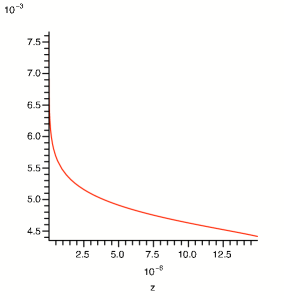
Figure 2: The behavior of the relative phase $\Delta\phi$ in the geometric phase for $p=10$.

The graph in fig. 2 represents the dependence of $\Delta\phi$ as a function of $z=\alpha^{-8}$ in the large radius phase $0<z<4$ for $p=10$. Note that it decreases monotonically from 0.0075 to 0.0044 as we approach the conifold point. Using formulas (A.28), we find that in the LG phase $0<\alpha<4$, $\Delta\Phi$ also decreases monotonically until it reaches the value $0.027$ at the LG point. One can also calculate the values of $\Delta\phi$ along a small circular contour surrounding the conifold, confirming that it varies continuously in this region. Since $\Delta\phi<1$, everywhere on the real axis, we conclude that the magnetized brane ${\underline{\CO_{C}}}(q)$ is stable with respect to the decay channel (A.24).

The analysis of other decay channels is very similar. Another decay channel is given by the following short exact sequence

$$0\to\CO_{D}(-C)(q)\to\CO_{D}(q)\to\CO_{C}(q)\to 0$$ (A.29)

where $D$ is a divisor on $X$ in the linear system $\eta_{1}$ containing $C$. Then, an analogous computation yields a similar variation of $\Delta\phi$ on the real axis, except that the maximum value is approximatively $0.015$ and it decreases monotonically to $0.008$ at the LG point. Therefore the magnetized brane is also stable with respect to the decay (A.29). In principle there could exit other decay channels, perhaps described by more exotic triangles in the derived category. A systematic analysis would take us too far afield, so we will simply assume that the magnetized branes are stable at the LG point based on the evidence presented so far. A rigorous proof of stability is not within the reach of current $\Pi$-stability techniques.

References

- [1] R. Blumenhagen, D. Lust, and T. R. Taylor, “Moduli stabilization in chiral type IIB orientifold models with fluxes,” Nucl. Phys. B663 (2003) 319–342, hep-th/0303016.
- [2] J. F. G. Cascales and A. M. Uranga, “Chiral 4d string vacua with D-branes and moduli stabilization,” hep-th/0311250.
- [3] J. F. G. Cascales and A. M. Uranga, “Chiral 4d N = 1 string vacua with D-branes and NSNS and RR fluxes,” JHEP 05 (2003) 011, hep-th/0303024.
- [4] M. Larosa and G. Pradisi, “Magnetized four-dimensional Z(2) x Z(2) orientifolds,” Nucl. Phys. B667 (2003) 261–309, hep-th/0305224.
- [5] D. Cremades, L. E. Ibanez, and F. Marchesano, “Computing Yukawa couplings from magnetized extra dimensions,” JHEP 05 (2004) 079, hep-th/0404229.
- [6] A. Font and L. E. Ibanez, “SUSY-breaking soft terms in a MSSM magnetized D7-brane model,” JHEP 03 (2005) 040, hep-th/0412150.
- [7] M. Cvetic and T. Liu, “Supersymmetric Standard Models, Flux Compactification and Moduli Stabilization,” Phys. Lett. B610 (2005) 122–128, hep-th/0409032.
- [8] D. Lust, S. Reffert, and S. Stieberger, “MSSM with soft SUSY breaking terms from D7-branes with fluxes,” Nucl. Phys. B727 (2005) 264–300, hep-th/0410074.
- [9] F. Marchesano and G. Shiu, “Building MSSM flux vacua,” JHEP 11 (2004) 041, hep-th/0409132.
- [10] F. Marchesano and G. Shiu, “MSSM vacua from flux compactifications,” Phys. Rev. D71 (2005) 011701, hep-th/0408059.
- [11] M. Cvetic, T. Li, and T. Liu, “Standard-like models as type IIB flux vacua,” Phys. Rev. D71 (2005) 106008, hep-th/0501041.
- [12] C. P. Burgess, R. Kallosh, and F. Quevedo, “de Sitter string vacua from supersymmetric D-terms,” JHEP 10 (2003) 056, hep-th/0309187.
- [13] I. Antoniadis and T. Maillard, “Moduli stabilization from magnetic fluxes in type I string theory,” Nucl. Phys. B716 (2005) 3–32, hep-th/0412008.
- [14] B. Kors and P. Nath, “Hierarchically split supersymmetry with Fayet-Iliopoulos D- terms in string theory,” Nucl. Phys. B711 (2005) 112–132, hep-th/0411201.
- [15] I. Antoniadis, A. Kumar, and T. Maillard, “Moduli stabilization with open and closed string fluxes,” hep-th/0505260.
- [16] E. Dudas and S. K. Vempati, “General soft terms from supergravity including D-terms,” hep-ph/0506029.
- [17] E. Dudas and S. K. Vempati, “Large D-terms, hierarchical soft spectra and moduli stabilisation,” Nucl. Phys. B727 (2005) 139–162, hep-th/0506172.
- [18] M. P. Garcia del Moral, “A new mechanism of Kahler moduli stabilization in type IIB theory,” hep-th/0506116.
- [19] R. Blumenhagen, G. Honecker, and T. Weigand, “Supersymmetric (non-)abelian bundles in the type I and SO(32) heterotic string,” JHEP 08 (2005) 009, hep-th/0507041.
- [20] R. Blumenhagen, F. Gmeiner, G. Honecker, D. Lust, and T. Weigand, “The statistics of supersymmetric D-brane models,” Nucl. Phys. B713 (2005) 83–135, hep-th/0411173.
- [21] F. Gmeiner, R. Blumenhagen, G. Honecker, D. Lust, and T. Weigand, “One in a billion: MSSM-like D-brane statistics,” JHEP 01 (2006) 004, hep-th/0510170.
- [22] F. Gmeiner, “Standard model statistics of a type II orientifold,” hep-th/0512190.
- [23] J. Gomis, F. Marchesano, and D. Mateos, “An open string landscape,” JHEP 11 (2005) 021, hep-th/0506179.
- [24] B. Acharya, M. Aganagic, K. Hori, and C. Vafa, “Orientifolds, mirror symmetry and superpotentials,” hep-th/0202208.
- [25] I. Brunner and K. Hori, “Orientifolds and mirror symmetry,” JHEP 11 (2004) 005, hep-th/0303135.
- [26] I. Brunner, K. Hori, K. Hosomichi, and J. Walcher, “Orientifolds of Gepner models,” hep-th/0401137.
- [27] T. W. Grimm and J. Louis, “The effective action of type IIA Calabi-Yau orientifolds,” Nucl. Phys. B718 (2005) 153–202, hep-th/0412277.
- [28] K. Behrndt and M. Cvetic, “General N = 1 supersymmetric flux vacua of (massive) type IIA string theory,” Phys. Rev. Lett. 95 (2005) 021601, hep-th/0403049.
- [29] J.-P. Derendinger, C. Kounnas, P. M. Petropoulos, and F. Zwirner, “Superpotentials in IIA compactifications with general fluxes,” Nucl. Phys. B715 (2005) 211–233, hep-th/0411276.
- [30] S. Kachru and A.-K. Kashani-Poor, “Moduli potentials in type IIA compactifications with RR and NS flux,” JHEP 03 (2005) 066, hep-th/0411279.
- [31] P. G. Camara, A. Font, and L. E. Ibanez, “Fluxes, moduli fixing and MSSM-like vacua in a simple IIA orientifold,” JHEP 09 (2005) 013, hep-th/0506066.
- [32] P. G. Camara, “Fluxes, moduli fixing and MSSM-like vacua in type IIA string theory,” hep-th/0512239.
- [33] O. DeWolfe, A. Giryavets, S. Kachru, and W. Taylor, “Type IIA moduli stabilization,” JHEP 07 (2005) 066, hep-th/0505160.
- [34] T. House and E. Palti, “Effective action of (massive) IIA on manifolds with SU(3) structure,” Phys. Rev. D72 (2005) 026004, hep-th/0505177.
- [35] G. Villadoro and F. Zwirner, “N = 1 effective potential from dual type-IIA D6/O6 orientifolds with general fluxes,” JHEP 06 (2005) 047, hep-th/0503169.
- [36] P. Berglund and P. Mayr, “Non-perturbative superpotentials in F-theory and string duality,” hep-th/0504058.
- [37] S. K. Donaldson and R. P. Thomas, “Gauge theory in higher dimensions,”. Prepared for Conference on Geometric Issues in Foundations of Science in honor of Sir Roger Penrose’s 65th Birthday, Oxford, England, 25-29 Jun 1996.
- [38] E. Witten, “Branes and the dynamics of QCD,” Nucl. Phys. B507 (1997) 658–690, hep-th/9706109.
- [39] W. Lerche, P. Mayr, and N. Warner, “N = 1 special geometry, mixed Hodge variations and toric geometry,” hep-th/0208039.
- [40] W. Lerche, P. Mayr, and N. Warner, “Holomorphic N = 1 special geometry of open-closed type II strings,” hep-th/0207259.
- [41] H. Clemens, “Cohomology and Obstructions II: Curves on K-trivial threefolds,” 2002.
- [42] D.-E. Diaconescu, R. Donagi, and T. Pantev, “Geometric transitions and mixed Hodge structures,” hep-th/0506195.
- [43] S. Kachru, R. Kallosh, A. Linde, and S. P. Trivedi, “De Sitter vacua in string theory,” Phys. Rev. D68 (2003) 046005, hep-th/0301240.
- [44] C. Escoda, M. Gomez-Reino, and F. Quevedo, “Saltatory de Sitter string vacua,” JHEP 11 (2003) 065, hep-th/0307160.
- [45] A. Saltman and E. Silverstein, “The scaling of the no-scale potential and de Sitter model building,” JHEP 11 (2004) 066, hep-th/0402135.
- [46] A. Saltman and E. Silverstein, “A new handle on de Sitter compactifications,” JHEP 01 (2006) 139, hep-th/0411271.
- [47] M. Becker, G. Curio, and A. Krause, “De Sitter vacua from heterotic M-theory,” Nucl. Phys. B693 (2004) 223–260, hep-th/0403027.
- [48] E. I. Buchbinder, “Raising anti de Sitter vacua to de Sitter vacua in heterotic M-theory,” Phys. Rev. D70 (2004) 066008, hep-th/0406101.
- [49] F. Saueressig, U. Theis, and S. Vandoren, “On de Sitter vacua in type IIA orientifold compactifications,” Phys. Lett. B633 (2006) 125–128, hep-th/0506181.
- [50] G. Villadoro and F. Zwirner, “D terms from D-branes, gauge invariance and moduli stabilization in flux compactifications,” hep-th/0602120.
- [51] L. Martucci, “D-branes on general N = 1 backgrounds: Superpotentials and D-terms,” hep-th/0602129.
- [52] T. W. Grimm and J. Louis, “The effective action of N = 1 Calabi-Yau orientifolds,” Nucl. Phys. B699 (2004) 387–426, hep-th/0403067.
- [53] A. Giryavets, S. Kachru, P. K. Tripathy, and S. P. Trivedi, “Flux compactifications on Calabi-Yau threefolds,” JHEP 04 (2004) 003, hep-th/0312104.
- [54] A. Font, “Periods and duality symmetries in Calabi-Yau compactifications,” Nucl. Phys. B391 (1993) 358–388, hep-th/9203084.
- [55] A. Klemm and S. Theisen, “Considerations of one modulus Calabi-Yau compactifications: Picard-Fuchs equations, Kahler potentials and mirror maps,” Nucl. Phys. B389 (1993) 153–180, hep-th/9205041.
- [56] P. Berglund et al., “Periods for Calabi-Yau and Landau-Ginzburg vacua,” Nucl. Phys. B419 (1994) 352–403, hep-th/9308005.
- [57] S. Gukov, C. Vafa, and E. Witten, “CFT’s from Calabi-Yau four-folds,” Nucl. Phys. B584 (2000) 69–108, hep-th/9906070.
- [58] S. Gukov, “Solitons, superpotentials and calibrations,” Nucl. Phys. B574 (2000) 169–188, hep-th/9911011.
- [59] M. Grana, “Flux compactifications in string theory: A comprehensive review,” Phys. Rept. 423 (2006) 91–158, hep-th/0509003.
- [60] C. P. Burgess, C. Escoda, and F. Quevedo, “Nonrenormalization of flux superpotentials in string theory,” hep-th/0510213.
- [61] S. Gurrieri, J. Louis, A. Micu, and D. Waldram, “Mirror symmetry in generalized Calabi-Yau compactifications,” Nucl. Phys. B654 (2003) 61–113, hep-th/0211102.
- [62] M. R. Douglas, B. Fiol, and C. Romelsberger, “Stability and BPS branes,” JHEP 09 (2005) 006, hep-th/0002037.
- [63] M. R. Douglas, “D-branes, categories and N = 1 supersymmetry,” J. Math. Phys. 42 (2001) 2818–2843, hep-th/0011017.
- [64] P. S. Aspinwall and M. R. Douglas, “D-brane stability and monodromy,” JHEP 05 (2002) 031, hep-th/0110071.
- [65] M. Grana, T. W. Grimm, H. Jockers, and J. Louis, “Soft supersymmetry breaking in Calabi-Yau orientifolds with D-branes and fluxes,” Nucl. Phys. B690 (2004) 21–61, hep-th/0312232.
- [66] D. Lust, S. Reffert, and S. Stieberger, “Flux-induced soft supersymmetry breaking in chiral type IIb orientifolds with D3/D7-branes,” Nucl. Phys. B706 (2005) 3–52, hep-th/0406092.
- [67] D. Lust, P. Mayr, S. Reffert, and S. Stieberger, “F-theory flux, destabilization of orientifolds and soft terms on D7-branes,” Nucl. Phys. B732 (2006) 243–290, hep-th/0501139.
- [68] H. Jockers and J. Louis, “The effective action of D7-branes in N = 1 Calabi-Yau orientifolds,” Nucl. Phys. B705 (2005) 167–211, hep-th/0409098.
- [69] H. Jockers and J. Louis, “D-terms and F-terms from D7-brane fluxes,” Nucl. Phys. B718 (2005) 203–246, hep-th/0502059.
- [70] D. Lust, P. Mayr, R. Richter, and S. Stieberger, “Scattering of gauge, matter, and moduli fields from intersecting branes,” Nucl. Phys. B696 (2004) 205–250, hep-th/0404134.
- [71] M. Bertolini, M. Billo, A. Lerda, J. F. Morales, and R. Russo, “Brane world effective actions for D-branes with fluxes,” hep-th/0512067.
- [72] M. R. Douglas and G. W. Moore, “D-branes, Quivers, and ALE Instantons,” hep-th/9603167.
- [73] S. Kachru and J. McGreevy, “Supersymmetric three-cycles and (super)symmetry breaking,” Phys. Rev. D61 (2000) 026001, hep-th/9908135.
- [74] J. A. Harvey, D. Kutasov, E. J. Martinec, and G. W. Moore, “Localized tachyons and RG flows,” hep-th/0111154.
- [75] A. Lawrence and J. McGreevy, “D-terms and D-strings in open string models,” JHEP 10 (2004) 056, hep-th/0409284.
- [76] R. Blumenhagen, V. Braun, B. Kors, and D. Lust, “Orientifolds of K3 and Calabi-Yau manifolds with intersecting D-branes,” JHEP 07 (2002) 026, hep-th/0206038.
- [77] D. Lust, “Intersecting brane worlds: A path to the standard model?,” Class. Quant. Grav. 21 (2004) S1399–1424, hep-th/0401156.
- [78] D.-E. Diaconescu, B. Florea, S. Kachru, and P. Svrcek, “Gauge - mediated supersymmetry breaking in string compactifications,” hep-th/0512170.
- [79] M. R. Douglas, B. Fiol, and C. Romelsberger, “The spectrum of BPS branes on a noncompact Calabi-Yau,” JHEP 09 (2005) 057, hep-th/0003263.
- [80] T. Bridgeland, “Stability conditions on triangulated categories,” math.AG/0212237.
- [81] T. Bridgeland, “Stability conditions on non-compact Calabi-Yau threefold,” math.AG/0509048.
- [82] M. Dine, N. Seiberg, and E. Witten, “Fayet-Iliopoulos Terms in String Theory,” Nucl. Phys. B289 (1987) 589.
- [83] M. Dine, I. Ichinose, and N. Seiberg, “F Terms and D Terms in string theory,” Nucl. Phys. B293 (1987) 253.
- [84] P. Binetruy, G. Dvali, R. Kallosh, and A. Van Proeyen, “Fayet-Iliopoulos terms in supergravity and cosmology,” Class. Quant. Grav. 21 (2004) 3137–3170, hep-th/0402046.
- [85] D. Z. Freedman and B. Kors, “Kaehler anomalies, Fayet-Iliopoulos couplings, and flux vacua,” hep-th/0509217.
- [86] B. Kors and P. Nath, “Effective action and soft supersymmetry breaking for intersecting D-brane models,” Nucl. Phys. B681 (2004) 77–119, hep-th/0309167.
- [87] G. W. Moore and E. Witten, “Self-duality, Ramond-Ramond fields, and K-theory,” JHEP 05 (2000) 032, hep-th/9912279.
- [88] D. S. Freed and E. Witten, “Anomalies in string theory with D-branes,” hep-th/9907189.
- [89] G. Villadoro and F. Zwirner, “de Sitter vacua via consistent D-terms,” Phys. Rev. Lett. 95 (2005) 231602, hep-th/0508167.
- [90] J. Shelton, W. Taylor, and B. Wecht, “Nongeometric flux compactifications,” JHEP 10 (2005) 085, hep-th/0508133.
- [91] G. Aldazabal, P. G. Camara, A. Font, and L. E. Ibanez, “More Dual Fluxes and Moduli Fixing,” hep-th/0602089.
- [92] J. M. Maldacena and C. Nunez, “Supergravity description of field theories on curved manifolds and a no go theorem,” Int. J. Mod. Phys. A16 (2001) 822–855, hep-th/0007018.
- [93] S. Ashok and M. R. Douglas, “Counting flux vacua,” JHEP 01 (2004) 060, hep-th/0307049.
- [94] M. R. Douglas, B. Shiffman, and S. Zelditch, “Critical points and supersymmetric vacua, II: Asymptotics and extremal metrics,” 2004.
- [95] F. Denef and M. R. Douglas, “Distributions of nonsupersymmetric flux vacua,” JHEP 03 (2005) 061, hep-th/0411183.
- [96] F. Denef and M. R. Douglas, “Distributions of flux vacua,” JHEP 05 (2004) 072, hep-th/0404116.
- [97] M. R. Douglas, “Basic results in vacuum statistics,” Comptes Rendus Physique 5 (2004) 965–977, hep-th/0409207.
- [98] O. DeWolfe, A. Giryavets, S. Kachru, and W. Taylor, “Enumerating flux vacua with enhanced symmetries,” JHEP 02 (2005) 037, hep-th/0411061.
- [99] B. S. Acharya, F. Denef, and R. Valandro, “Statistics of M theory vacua,” JHEP 06 (2005) 056, hep-th/0502060.
- [100] B. S. Acharya, “A moduli fixing mechanism in M theory,” hep-th/0212294.
- [101] F. Denef, M. R. Douglas, and B. Florea, “Building a better racetrack,” JHEP 06 (2004) 034, hep-th/0404257.
- [102] F. Denef, M. R. Douglas, B. Florea, A. Grassi, and S. Kachru, “Fixing all moduli in a simple F-theory compactification,” hep-th/0503124.
- [103] D. Lust, S. Reffert, W. Schulgin, and S. Stieberger, “Moduli stabilization in type IIB orientifolds. I: Orbifold limits,” hep-th/0506090.
- [104] S. Reffert and E. Scheidegger, “Moduli stabilization in toroidal type IIB orientifolds,” hep-th/0512287.
- [105] V. Balasubramanian, P. Berglund, J. P. Conlon, and F. Quevedo, “Systematics of moduli stabilisation in Calabi-Yau flux compactifications,” JHEP 03 (2005) 007, hep-th/0502058.
- [106] P. S. Aspinwall, “A point’s point of view of stringy geometry,” JHEP 01 (2003) 002, hep-th/0203111.