Entanglement Entropy in Critical Phenomena and Analogue Models of Quantum Gravity

Abstract

A general geometrical structure of the entanglement entropy for spatial partition of a relativistic QFT system is established by using methods of the effective gravity action and the spectral geometry. A special attention is payed to the subleading terms in the entropy in different dimensions and to behaviour in different states. It is conjectured, on the base of relation between the entropy and the action, that in a fundamental theory the ground state entanglement entropy per unit area equals $1/(4G_{N})$, where $G_{N}$ is the Newton constant in the low-energy gravity sector of the theory. The conjecture opens a new avenue in analogue gravity models. For instance, in higher dimensional condensed matter systems, which near a critical point are described by relativistic QFT’s, the entanglement entropy density defines an effective gravitational coupling. By studying the properties of this constant one can get new insights in quantum gravity phenomena, such as the universality of the low-energy physics, the renormalization group behavior of $G_{N}$, the statistical meaning of the Bekenstein-Hawking entropy.

I Fundamental entanglement

I.1 General properties

Quantum entanglement is an important physical phenomenon in which the quantum states of several objects cannot be described independently, even if the objects are spatially separated. Quantum entanglement is used in different research areas Pres . In quantum information theory entangled states are a valuable source of processing the information. Quantum entanglement also plays an important role in properties of strongly correlated many-body systems and in collective phenomena such as quantum phase transitions. In quantum gravity the entanglement may be a key for understanding the mystery of the black hole entropy.

The entanglement can be quantified by an entropy. One can define it as the measure of the information about quantum states which is lost when these states cannot be observed. In many-body systems, which are the subject of the present work, ”observable” and ”unobservable” states can be located in different regions. Consider, for instance, a lattice of spins being in a quantum state characterized by a density matrix $\hat{\rho}$. Suppose that the lattice is divided into regions $A$ and $B$ with a common boundary $\cal B$. The entanglement between the two regions can be described by the reduced density matrix

$$\hat{{\rho}}_{B}=\mbox{Tr}_{A}\hat{\rho}~{}~{},$$

where the trace is taken over the states of spin operators at the lattice sites in the region $A$. The entanglement entropy in the region $B$ is defined as the von Neumann entropy

$$S_{B}=-\mbox{Tr}_{B}\hat{{\rho}}_{B}\ln\hat{{\rho}}_{B}~{}~{}.$$ (1)

Analogously one can define the entanglement entropy $S_{A}$ in the region $A$ by tracing the density matrix over the states located in the region $B$. If the system is in a pure state $|\psi\rangle$, i.e. $\hat{{\rho}}=|\psi\rangle\langle\psi|$, it is not difficult to show that $S_{A}=S_{B}$, see Sr:93 .

It has been observed long ago Sr:93 ,BKLS (see also recent works Plenio1 , Plenio2 ), that in lattice models representing a discrete version of a relativistic quantum field theory (QFT) the ground state entanglement entropy in the leading order is proportional to the area $\cal A$ of $\cal B$,

$$S=S_{B}\sim{{\cal A}\over\varrho^{D-2}}~{}~{}.$$ (2)

Here $\varrho$ is the lattice spacing and $D$ is the number of spacetimes dimensions (it is assumed that $D>2$). This geometrical property of $S$ follows from the fact that field excitations in different regions are correlated across the boundary.

I.2 Black hole entropy

If $\varrho$ is identified with the Planck length $l_{Pl}$, (2) looks very similar to the Bekenstein-Hawking entropy of a black hole

$$S^{BH}={{\cal A}_{H}\over 4G_{N}}~{}~{}.$$ (3)

Here ${\cal A}_{H}$ is the area surface of the black hole horizon and $G_{N}$ is the Newton constant, $G_{N}=l_{Pl}^{D-2}$. The similarity of the two entropies suggests that $S^{BH}$ may be an entanglement entropy, as was first pointed out in Sr:93 ,BKLS . An external observer, who is at rest with respect to a black hole, never sees what happens inside the horizon. Because the observer perceives the vacuum excitations in a mixed state it is natural to assume that $S^{BH}$ measures the loss of the information inside the horizon.

The reduced density matrix for a black hole is thermal Israel:76 . Thus, the entanglement entropy coincides with the entropy of a thermal atmosphere around the black hole horizon (see FrFu:98 for a review of different interpretations of $S^{BH}$ in terms of the entropy of quantum excitations). However, relation between $S^{BH}$ and the entropy of entanglement (or thermal entropy) is non-trivial because $S$ is divergent. In the lattice regularization (2) diverges in the continuum limit when $\varrho\rightarrow 0$. It was pointed out in SuUg:94 , CaWi:94 that the divergences in $S$ are the standard ultraviolet divergences. If the entropy of thermal atmosphere is considered as a quantum correction to $S^{BH}$ the divergences can be eliminated in the course of renormalization of the gravitational coupling.

A deep connection between the divergences in $S$ and the divergences in the quantum effective action has been established latter for different field species at the one-loop level FrFu:98 . This connection is very important. Suppose, following the original idea by Sakharov Sakh , that the Einstein action is entirely induced by quantum effects of some underlying fundamental theory. Because the Newton constant in this case has a pure quantum origin, so does the entropy $S^{BH}$. The hypothesis is that the entropy of a black hole in such a theory is an entanglement entropy of fundamental quantum excitations which induce low-energy gravity dynamics Jaco:94 –FF:97 .

The mechanism of generation of the black hole entropy in induced gravity may be quite general and, in particular, it can be realized in string theory MHS . In string theory the low-energy effective gravity action appears from the tree-level diagrams of closed strings. From the point of view of open strings these are one-loop diagrams. Thus, the gravity action as well as the Bekenstein-Hawking entropy can be interpreted as a pure loop effect. Another argument in favour of entanglement interpretation of black hole entropy comes from analysis of string theory on asymptotically anti-de Sitter backgrounds and its duality to a conformal field theory (CFT) Mald ,BEY .

I.3 Entanglement entropy in fundamental theories

The purpose of the present work is to look at these results from a different perspective. Suppose the underlying fundamental theory of quantum gravity is known. This can be a string–$D$-brane theory or some other theory which correctly describes the observable particle physics and gravitational effects. Consider a low-energy limit of this theory and the entanglement entropy $S$ in the ground state for partition of the system in Minkowsky spacetime by a plane. It is assumed that $S$ measures entanglement of all genuine microscopical degrees of freedom of the fundamental theory (which may not coincide with the low-energy fields). We call such quantity the fundamental entanglement entropy.

Because the space is infinite it is convenient to discuss the density of $S$ per unit area. Let us denote this quantity by ${\cal S}$. We make a conjecture that the density of the fundamental entanglement entropy is finite and is given precisely by the relation

$${\cal S}={1\over 4G_{N}}~{}~{},$$ (4)

where $G_{N}$ is the Newton constant in the low-energy gravity sector of the theory. The conjecture is based on the above mentioned arguments:

i) in a fundamental theory the cutoff parameter $\varrho$ in (2) should be of the order of the Planck length;

ii) there are evidences that the Bekenstein-Hawking entropy (3) is the entanglement entropy for partition of the system by the horizon.

In what follows we discuss a more formal argument in favour of (4). It is based on the observation that the black hole entropy and the entropy of entanglement are derived in a unique way from the effective gravity action.

Relation (4) has a number of interesting consequences. One of them is that the definition of $G_{N}$ becomes not only the subject of gravitational physics. The flat space entanglement is an alternative source of information about the Newton constant. (In a certain sense the situation with different definitions of $G_{N}$ can be compared with ”gravitational” and the ”inertional” notions of the mass.)

In this paper we pay attention to the fact that relation (4) can be used to study the properties of the gravitational coupling by carrying the computations of the entanglement entropy in condensed matter systems. There are higher-dimensional condensed matter systems which near a critical point corresponding to a second order phase transition are described by relativistic QFT’s which contain massive fields. The class of Ising models is one of such examples. The QFT’s in these systems are analogous to low-energy limit of the fundamental theory. The relativistic covariance guarantees that the entanglement entropy density in the near-critical regime determines an effective gravitational coupling by the same equation as Eq. (4). The lattice spacing in the underlying theory serves as a cutoff. Hence the entanglement entropy is finite and can be calculated by using analytical and numerical methods. This enables one to pose different questions about properties of $G_{N}$ and try to find the answers in gravity analogs.

I.4 Outline of the paper

The rest part of the paper is organized as follows. Section II is devoted to the entanglement entropy in relativistic QFT’s. The Section starts with discussion of one-dimensional spin models which serve as an illustration. We then establish connection between the entanglement entropy $S$ in relativistic QFT’s and the effective gravity action, and use methods of the spectral geometry for derivation of $S$. By studying the theories in a cubic region we find a geometric form of $S$ in different dimensions, at zero and high temperatures. We pay a special attention at boundary effects. Our result for the ground state entanglement in four-dimensional space-times looks as follows:

$$S\sim{{\cal A}\over\varrho^{2}}+{{\cal L}\over\varrho}+{\cal C}\ln\varrho~{}~{}~{},$$ (5)

where $\cal A$ is the area of the separating surface $\cal B$ and $\cal L$ is the length of the boundary of $\cal B$. The last term in $S$ has a topological form. It depends on the number $\cal C$ of sharp corners (vertexes) of the boundary of $\cal B$ and does not change under smooth deformations of $\cal B$. Calculation of the subleading terms in (5) is the new result.

Relation of $S$ to the Bekenstein-Hawking entropy in induced gravity models in four dimensions is discussed in Section III. We also discuss the concept of gravity analogs and possible models which can be used to study properties of the gravitational coupling on the base of relation (4). There are several topics which can be pursued by using simulations in the new class of gravity analogs. Some of them such as the renormalization group behavior of $G_{N}$, the universality of the low-energy physics and the statistical meaning of the Bekenstein-Hawking entropy are listed in Section IV.

II Entanglement in relativistic field theories

II.1 One-dimensional spin chains

We begin with discussion of the properties of the entanglement entropy in one-dimensional spin chains. Consider as a simplest example the entanglement entropy for a block of spins in the Ising model. The Hamiltonian of the model is

$$H=\sum_{i=1}^{N}\left(\sigma_{i}^{x}\sigma_{i+1}^{x}+\lambda\sigma_{i}^{z}\right)~{}~{}~{},$$ (6)

where $N$ is the number of spins and $\sigma_{i}^{x},\sigma_{i}^{z}$ are the Pauli matrices. Parameter $\lambda$ is the strength of external magnetic field. At zero temperature the Ising chain has a second order phase transition at the critical value $\lambda=1$.

As is known, there is a unitary transformation (the Jordan-Wigner transformation) which maps the spin models like (6) to one-dimensional models with two spinless fermions. This transformation can be used to diagonalize the Hamiltonian.

The entanglement entropy can be investigated for the ground state when the chain is separated into two blocks of contiguous spins of equal sizes $N/2$. Suppose that $\lambda$ is fixed and $N$ varies ($N$ is much larger than the correlation length). The behaviour of $S$ has been studied in two regimes crit1 . In the off-critical regime, $\lambda\neq 1$ and $|\lambda-1|\ll 1$, the entropy at large $N$ reaches the saturation value

$$S(N,\lambda)=-\frac{1}{6}\log_{2}|\lambda-1|~{}~{}.$$ (7)

In the critical regime, $\lambda=1$, the entropy does not reach the saturation and behaves at large $N$ as

$$S(N,\lambda)\simeq\frac{1}{6}\log_{2}N/2~{}~{}~{}.$$ (8)

The explanation of these results is based on the fact that in the continuous limit, $N\rightarrow\infty$, the Ising model near the critical point corresponds to a quantum field theory with two fermion fields whose mass $m$ (or the inverse correlation length $\xi^{-1}$) is monotonically related to $|\lambda-1|$. In the critical regime $m$ vanishes and one has a conformal field theory with two massless fermions each having the central charge $1/2$.

Formulae (7), (8) are quite general. They have been verified in other exactly solvable one-dimensional statistical models (XXZ, XY and other models) which generalize the Izing chain (6), see crit1 –crit4 and a review of results in Rico . To discuss the continuum limit in lattice models it is convenient to introduce the lattice spacing $\varrho$. Then the number of spins $N$ defines the size of the system $L=N\varrho$. In the systems separated into two equal parts the entropy at the critical points behaves as

$$S\simeq\frac{c}{6}\ln{L\over 2\varrho}~{}~{},$$ (9)

where $c$ is a total central charge of the corresponding effective two-dimensional conformal theory. Near the critical point the entropy behaves as

$$S\simeq\frac{c}{6}\ln{1\over\varrho m}~{}~{},$$ (10)

where $m$ is the corresponding inverse correlation length. From the point of view of QFT $\varrho$ is the ultraviolet cutoff parameter.

II.2 Entanglement entropy and effective gravity action

There are different ways to derive (9), (10) by QFT methods. Our purpose is to show how it can be done by using the effective action approach. We first start with a theory in a flat spacetime with arbitrary number of dimensions $D$ and then focus on theories in $D=2,3$, and 4.

The entanglement entropy (1) for a lattice system discussed in Section I.A can be rewritten as

$$S_{B}=-\lim_{n\rightarrow 1}~{}{\partial\over\partial n}\mbox{Tr}_{B}~{}\hat{{\rho}}_{B}^{~{}n}~{}~{}~{}.$$ (11)

Suppose that near a critical point the system is equivalent to a QFT with field variables $\phi$ whose dynamics is determined by the action $I_{E}[\phi]$. The density matrix $\hat{{\rho}}_{B}$ in the configuration representation depends on variables $\phi_{B}$ in the region $B$. We consider the system at a finite temperature $T$. The result for the ground state entanglement can be obtained in the limit $T\rightarrow 0$. The matrix elements of $\hat{{\rho}}_{B}$ can be described in terms of the Euclidean path integral

$$\langle\phi^{\prime}_{B}|\hat{{\rho}}_{B}|\phi_{B}\rangle={\cal N}^{-1}\int^{\phi=\phi^{\prime}_{B}}_{\phi=\phi_{B}}[D\tilde{\phi}]~{}e^{-I_{E}[\phi]}~{}~{}~{},$$ (12)

where $\cal N$ is a normalization coefficient introduced to satisfy the condition $\mbox{Tr}_{B}~{}\hat{{\rho}}_{B}=1$. The classical action $I_{E}[\phi]$ is defined on a Euclidean space with Euclidean time $\tau$ compactified on a circle of length $T^{-1}$. To be more specific suppose that the partition of the space is done orthogonally to one of the spatial coordinates, say $x^{1}$. Then regions $A$ and $B$ can be defined, respectively, as $-L/2<x^{1}<0$ and $0<x^{1}<L/2$, the separating surface is located at $x^{1}=0$. Relative sizes of $A$ and $B$ can be arbitrary in general. The integration in (12) goes over field configurations $\phi$ with the boundary conditions

$$\phi(x^{1},...,x^{D-1},\tau=0)=\phi_{B}(x^{1},...,x^{D-1})~{}~{},$$

$$\phi(x^{1},...,x^{D-1},\tau=T^{-1})=\phi^{\prime}_{B}(x^{1},...,x^{D-1})~{}~{},$$

where $x^{1}$ takes values in the interval $(0,L/2)$.

Let us denote by ${\cal M}^{\prime}_{1}$ the space where the field configurations $\phi$ are given. It is easy to see how ${\cal M}^{\prime}_{1}$ looks in two dimensions. It is a cylinder (see the upper picture on Fig. 1) with coordinates $(x^{1},\tau)$ and a cut parallel to its axis, the length of the cut is equal to the length of the interval $B$. The field takes values $\phi_{B}$, $\phi_{B}^{\prime}$ on the lower and upper sides of the cut, respectively. In higher dimensions the cut is a $(D-2)$-dimensional hyperplane.

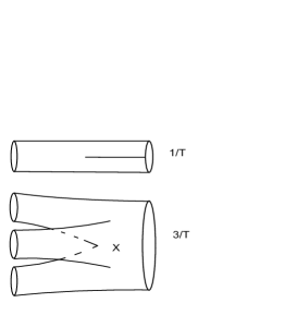
Figure 1: The upper picture shows ${\cal M}^{\prime}_{1}$ in two dimensions. It is a cylinder with the circumference length $T^{-1}$ and a cut along the axis. The space ${\cal M}_{3}$ is schematically drawn on the lower picture. It is obtained by gluing along the cuts of 3 copies of ${\cal M}^{\prime}_{1}$. The circumference length of the right boundary of ${\cal M}_{3}$ is $3T^{-1}$. The cuts meet at the point $X$ which is a conical singularity.

If the parameter $n$ in (11) is positive and integer the matrix elements of the operator $\hat{{\rho}}_{B}^{~{}n}$ can be represented by integral (12) where field variables are defined on a space ${\cal M}^{\prime}_{n}$ which is obtained by gluing $n$ copies of ${\cal M}^{\prime}_{1}$ along the cuts. ${\cal M}^{\prime}_{n}$ still has a single cut which disappears when one takes the trace, $\mbox{Tr}_{B}~{}\hat{{\rho}}_{B}^{~{}n}$. We denote the space obtained as a result of this procedure as ${\cal M}_{n}$. The lower picture on Fig. 1 shows ${\cal M}_{3}$ in two dimensions.

${\cal M}_{n}$ is locally flat but has a non-trivial topology. Its boundary in two dimensions consists of $n$ circles of the length $T^{-1}$ each and a circle of the length $nT^{-1}$. The important property is that ${\cal M}_{n}$ has a singularity at a hyper-surface where all $n$ cuts meet. For $n\geq 2$ each point on this hyper-surface is the conical singularity because a unit circle around it has the circumference length equal $2\pi n$.

The singular behaviour of ${\cal M}_{n}$ is easy to see in two dimensions. ${\cal M}_{n}$ has the same topology as a disk with $n$ holes. Thus, its Euler characteristic,

$$\chi[{\cal M}_{n}]={1\over 4\pi}\left[\int_{{\cal M}_{n}}R+2\int_{\partial{\cal M}_{n}}k\right]~{}~{},$$

equals $1-n$. The boundary $\partial{\cal M}_{n}$ of ${\cal M}_{n}$ consists of $n+1$ circles, each of which has a vanishing extrinsic curvature $k=0$. Therefore, the integral of the scalar curvature $R$ for ${\cal M}_{n}$ should be non-trivial for $n>1$,

$$\int_{{\cal M}_{n}}R=4\pi(1-n)~{}~{}.$$

The non-zero value of the integral is ensured by the conical singularity. If this point is located at $x=0$ the curvature is the distribution $R=4\pi(1-n)\delta^{(2)}(x)$, see, e.g. FS1 .

Let us introduce the parameter $\beta=2\pi n$ and rewrite (11) in another form following from (12),

$$S_{B}=\lim_{\beta\rightarrow 2\pi}~{}\left(\beta{\partial\over\partial\beta}-1\right)\Gamma(\beta)~{}~{}~{}.$$ (13)

$\Gamma(\beta)$ is the effective action defined by the path integral

$$e^{-\Gamma(\beta)}=\int[D\tilde{\phi}]~{}e^{-I_{E}[\phi,\beta]}~{}~{}~{},$$ (14)

where field variables are given on ${\cal M}_{n}$. $I_{E}[\phi,\beta]$ is the classical action on ${\cal M}_{n}$. The normalization of the integral (14) is fixed by the condition $\Gamma(2\pi)=-\ln{\cal N}$.

The operation with the parameter $\beta$ in (13) should be understood in the following way: one first computes $\Gamma(\beta)$ for $\beta=2\pi n$, and then replaces $\beta$ with a continuous parameter. This can be done even if ${\cal M}_{n}$ itself cannot be defined at arbitrary $\beta$.

If one defines a ”free energy” $F(\beta)=\Gamma(\beta)/\beta$ and interpretes $\beta$ as an inverse temperature, equation (13) formally coincides with the definition of the entropy in statistical mechanics. Note, that $\beta^{-1}$ is a ”geometrical temperature” which should not be confused with the physical temperature $T$.

II.3 Spectral geometry on ${\cal M}_{n}$

The expression of the entanglement entropy in terms of the effective action has a number of advantages. It enables one to reformulate the problem on the geometrical language and use powerful methods of the spectral geometry to study the form of the entropy.

Consider a Laplace operator $\Delta=-\nabla^{2}$ on ${\cal M}_{n}$ and the trace of its heat kernel, $\mbox{Tr}~{}e^{-t\Delta}$, where $t$ is a positive parameter. The spectral geometry relates the asymptotic of the trace at small $t$ to integral geometrical characteristics of ${\cal M}_{n}$,

$$\mbox{Tr}~{}e^{-t\Delta}\sim{1\over(4\pi t)^{D/2}}\sum_{n}a_{n}t^{n}~{}~{}~{},$$ (15)

where $n$ takes non-negative integer and half-integer values. The coefficients $a_{n}$ are expressed in terms of the powers of the Riemann tensor and its derivatives, and include boundary terms (see, e.g., Vass ). The coefficients also depend on the singularities of the background manifold such as jumps of the curvature, sharp corners, and so on. The effect of conical singularities appears starting with the coefficient $a_{1}$. For scalar and spinor Laplacians in two dimensions Furs:94b

$$a_{1}={\pi\over 3}\left({2\pi\over\beta}-{\beta\over 2\pi}\right)+\frac{1}{3}\int_{\partial{\cal M}}k~{}~{}~{}.$$ (16)

For spaces ${\cal M}_{n}$ like those shown on Fig. 1 the extrinsic curvature for each element of the boundary is zero and $a_{1}$ is determined only by the conical singularity. Other non-vanishing coefficients in the asymptotic expansion for the heat kernel on ${\cal M}_{n}$ in $D=2$ are

$$a_{0}=l\mbox{vol}({\cal M}_{n})=l{nL\over T}=l{\beta L\over 2\pi T}~{}~{}~{},$$ (17)

$$a_{1/2}=\sqrt{4\pi}b_{1/2}^{\pm}\int_{\partial{\cal M}_{n}}=\sqrt{4\pi}b_{1/2}^{\pm}{2n\over T}=\sqrt{4\pi}b_{1/2}^{\pm}{\beta\over\pi T}~{}~{}~{}.$$ (18)

For scalars and spinors $l=1$ and $l=2$, respectively. The numerical coefficients $b_{1/2}^{+}$ and $b_{1/2}^{-}=-b_{1/2}^{+}$ correspond, respectively, to the Dirichlet and Neumann conditions on the boundaries of ${\cal M}_{n}$. For the scalar Laplacian $b^{+}_{1}=-1/4$ and $b^{+}_{1}=-1/2$ for the spinor Laplacian. The non-trivial dependence on $\beta$ in the first term in the r.h.s. of (16) is the direct consequence of the conical singularity.

Figure 2: This figure shows division of a cube by a plane $\cal B$. The trace is taken over the states of a QFT in one of the halfs of the cube.

Consider now QFT in a $(D-1)$-dimensional cube with the Dirichlet or Neumann boundary conditions on its faces. Let $L$ be the length of the edge of the cube. Suppose we are interested in the entanglement entropy associated with the partition of the cube by a plane ${\cal B}$ which is orthogonal to one of the faces and divides the cube into two equal parts, as is shown on Fig. 2. Let us denote by ${\cal M}^{(D)}_{n}$ a $D$–dimensional manifold which appears in calculation of the entanglement entropy in terms of the effective action along the lines explained in Section II.B.

In two dimensions ${\cal M}^{(2)}_{n}$ is shown on Fig. 1. If $D>2$ the manifold ${\cal M}^{(D)}_{n}$ is the space product of ${\cal M}^{(2)}_{n}$ and $D-2$ intervals of the length $L$. For a scalar Laplace operator $\Delta^{(D)}$ on ${\cal M}^{(D)}_{n}$ one can write

$$\mbox{Tr}~{}e^{-t\Delta^{(D)}}=(K_{L}(t))^{D-2}~{}\mbox{Tr}~{}e^{-t\Delta^{(2)}}~{}~{}~{},$$ (19)

where $K_{L}(t)$ is the trace of the heat kernel of the Laplace operator on the interval Vass . The following asymptotics hold at small $t$ up to exponentially small terms

$$\mbox{Tr}~{}e^{-t\Delta^{(2)}}\sim{1\over 4\pi t}(a_{0}+a_{1/2}\sqrt{t}+a_{1}t)~{}~{}~{},$$ (20)

$$K_{L}(t)\sim{1\over\sqrt{4\pi t}}(L+2b_{1/2}^{\pm}\sqrt{4\pi t})~{}~{}~{},$$ (21)

where $a_{n}$ are given in (16)–(18). Therefore,

$$\mbox{Tr}~{}e^{-t\Delta^{(D)}}\sim{1\over(4\pi t)^{D/2}}\sum_{n=0}^{D/2}a_{n}^{(D)}t^{n}~{}~{}~{},$$ (22)

where coefficients $a_{n}^{(D)}$ can be found from (20), (21). One can check with the help of (16)–(18) that the first coefficients take the form

$$a_{0}^{(D)}={\beta\over 2\pi T}L^{D-1}=\mbox{vol}({\cal M}^{(D)}_{n})~{}~{}~{},$$ (23)

$$a_{1/2}^{(D)}=\sqrt{4\pi}b_{1/2}^{\pm}{\beta\over\pi T}(D-1)L^{D-2}=\sqrt{4\pi}b_{1/2}^{\pm}\int_{\partial{\cal M}^{(D)}_{n}}~{}~{}~{},$$ (24)

$$a_{1}^{(D)}={\pi\over 3}\left({2\pi\over\beta}-{\beta\over 2\pi}\right)L^{D-2}+$$

$$(\sqrt{4\pi}b_{1/2}^{\pm})^{2}{\beta\over\pi T}(D-1)(D-2)L^{D-3}~{}~{}~{},$$ (25)

$$a_{3/2}^{(D)}={\pi\over 3}\left({2\pi\over\beta}-{\beta\over 2\pi}\right)(\sqrt{4\pi}b_{1/2}^{\pm})2(D-2)L^{D-3}+$$

$$(\sqrt{4\pi}b_{1/2}^{\pm})^{3}{\beta\over\pi T}2^{2}{(D-1)!\over 3!(D-4)!}L^{D-4}~{}~{}~{},$$ (26)

$$a_{2}^{(D)}={\pi\over 3}\left({2\pi\over\beta}-{\beta\over 2\pi}\right)(\sqrt{4\pi}b_{1/2}^{\pm})^{2}2(D-2)(D-3)L^{D-4}+$$

$$(\sqrt{4\pi}b_{1/2}^{\pm})^{4}{\beta\over\pi T}2^{3}{(D-1)!\over 4!(D-5)!}L^{D-5}~{}~{}~{}.$$ (27)

The heat kernel coefficients for the spinor Laplacian have a similar structure and can be found in analogous way.

Although our computations have been done in a simple setting, the results can be easily generalized when ${\cal M}^{(D)}_{n}$ is an arbitrary curved manifold. We are particularly interested in the geometrical form of contributions to the heat kernel coefficients from the conical singularities because they yield a non-trivial value of the entanglement entropy. These contributions depend on the factor $((2\pi/\beta)-(\beta/2\pi))$ and appear in the coefficients $a_{n}$ with $n\geq 1$. The geometrical structures related to conical singularities in the coefficients $a_{1}$, $a_{3/2}$, and $a_{2}$ are, respectively,

$$L^{D-2}=\int_{\cal B}~{}\equiv{\cal A}~{}~{}~{},$$ (28)

$$2(D-2)L^{D-3}=\int_{\partial{\cal B}}\equiv{\cal L}~{}~{}~{},$$ (29)

$$2(D-2)(D-3)L^{D-4}=\int_{\mbox{\tiny{sing}}~{}\partial{\cal B}}\equiv{\cal C}~{}~{}~{}.$$ (30)

The separating surface $\cal B$ is a $(D-2)$–dimensional manifold. In general, it may have a boundary $\partial{\cal B}$ and the boundary may consist of different hypersurfaces where the curvature of $\partial{\cal B}$ has jumps. Integrals in the right hand sides of (29) and (30) are taken, respectively, over the boundary $\partial{\cal B}$ and codimension 1 singular hypersurfaces inside $\partial{\cal B}$. In the considered example of the theory in the hypercube, $\cal B$ is a square if $D=4$ (see Fig. 2). It has the area ${\cal A}=L^{2}$ if the edge length is $L$. Its boundary $\partial{\cal B}$ has the length $4L$ and consists of $4$ singular points, the vertexes of the square. If $\cal B$ is a $D-2$-dimensional hypercube, $2(D-2)$ is the number of its ”faces” and $2(D-2)(D-3)$ is the number of its ”edges”.

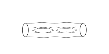
Figure 3: The manifold ${\cal M}^{(2)}_{3}$ is shown for computing the entanglement entropy $S_{B}$ at a finite temperature when the region $A$ consists of two internal disjoint intervals. ${\cal M}^{(2)}_{3}$ is obtained by gluing 4 copies of the manifold shown on Fig. 1. ${\cal M}^{(2)}_{3}$ has 4 conical singularities at branch points.

II.4 Effective action and the entropy

Let us show now how the geometrical structure of the entanglement entropy can be established by using the effective action. We consider, as an example, a free scalar field theory in a cube divided into two parts, Fig. 2. The effective action for a massive scalar field can be defined as follows

$$\Gamma=\frac{1}{2}\ln\det((\Delta+m^{2})\mu^{-2})\equiv-\frac{1}{2}\int_{\varrho^{2}}^{\infty}{dt\over t}\mbox{Tr}~{}e^{-t\Delta}e^{-tm^{2}}~{}~{},$$ (31)

where $\mu$ is a dimensional parameter. The right hand side of (31) gives the effective action in the Schwinger-De Witt representation. The parameter $\varrho$ is a ultraviolet cutoff which has a dimensionality of a length.

It is assumed that the correlation length $m^{-1}$ of the theory is much larger than $\varrho$. Let us also assume that $m^{-1}$ is much smaller than the size of the system $L$. In this case one can use for $\Gamma$ an approximation which can be obtained when the heat kernel is replaced by its asymptotic (22).

Here and in what follows we use instead $S_{B}$ the notation $S$ because in the considered examples the regions $A$ and $B$ are identical.

1. D=2

In two-dimensional theories

$$\Gamma\sim-{1\over 8\pi}\left[a_{0}^{(2)}\varrho^{-2}+2a_{1/2}^{(2)}\varrho^{-1}\right.$$

$$\left.+(m^{2}a_{0}^{(2)}-a_{1}^{(2)})\ln(m^{2}\varrho^{2})-(a_{0}^{(2)}m^{2}-a_{1/2}^{(2)}m\sqrt{\pi})\right]~{}~{}.$$ (32)

In this expression we drop all terms which vanish in the limit $\varrho\rightarrow 0$. To find the entropy one can apply (13) to (32) and use (23)–(25). It yields

$$S\sim-{1\over 12}\ln(m^{2}\varrho^{2})~{}~{}~{}.$$ (33)

If $\varrho$ is identified with the lattice spacing, this result coincides with computations in spin chains in the near critical regime, see (10). The central charge in the given case is $c=1$. Formula (33) is obtained for the partition of the interval into two parts. It can be easily generalized for more complicated cases when the regions $A$ and $B$ consist of several disjoint intervals. The effective action in this case is defined on a 2D manifold ${\cal M}^{(2)}_{n}$ with some number of handles. Figure 3 shows ${\cal M}^{(2)}_{3}$ for tracing the degrees of freedom in two disjoint internal intervals. As is easy to understand the number of conical singularities ${\cal N}_{c}$ of ${\cal M}^{(2)}_{n}$ equals the number of internal points of the intervals. Each conical singularity yields an independent contribution to the entropy. Thus, in general case the result in the right hand side of (33) has to be multiplied by ${\cal N}_{c}$ CaCa:04 .

2. D=3

In three-dimensional theories

$$\Gamma\sim-{1\over 16\pi^{3/2}}\left[\frac{2}{3}a_{0}^{(3)}\varrho^{-3}+a_{1/2}^{(3)}\varrho^{-2}+\right.$$

$$2(a_{1}^{(3)}-m^{2}a_{0}^{(3)})\varrho^{-1}-(a_{3/2}^{(3)}-m^{2}a_{1/2}^{(3)})\ln(m^{2}\varrho^{2})+$$

$$\left.\left({2\over 3\sqrt{\pi}}a_{0}^{(3)}m^{3}-a_{1/2}^{(3)}m^{2}-\sqrt{\pi}a_{1}^{(3)}m\right)\right]~{}~{}$$ (34)

and the entanglement entropy takes the form

$$S\sim{1\over 12\sqrt{\pi}}\left[\left({1\over\varrho}-{\sqrt{\pi}\over 2}m\right){\cal A}-b_{1/2}^{\pm}\ln(m^{2}\varrho^{2})~{}{\cal L}\right]~{}~{}~{},$$ (35)

where we used (28),(29). For the theory in the square ${\cal A}=L$, ${\cal L}=2$. The term in (35) which is proportional to ${\cal L}$ has the following property: it does not change under continuous deformation of the separation surface $\cal B$. This property is in agreement with a more general behaviour of the entanglement entropy in three-dimensional theories which has a topological part arising from short wavelength modes localized near the boundary of $\cal B$, see KiPr .

3. D=4

In four-dimensional theories

$$\Gamma\sim-{1\over 32\pi^{2}}\left[\frac{1}{2}a_{0}^{(4)}\varrho^{-4}+\frac{2}{3}a_{1/2}^{(4)}\varrho^{-3}+\right.$$

$$(a_{1}^{(4)}-m^{2}a_{0}^{(4)})\varrho^{-2}+2(a_{3/2}^{(4)}-m^{2}a_{1/2}^{(4)})\varrho^{-1}-$$

$$(a_{2}^{(4)}-m^{2}a_{1}^{(4)}+{m^{4}\over 2}a_{0}^{(4)})\ln(m^{2}\varrho^{2})+$$

$$\left.\left(\frac{3}{4}a_{0}^{(4)}m^{4}+{2\over 3\sqrt{\pi}}a_{1/2}^{(4)}m^{3}-a_{1}^{(4)}m^{2}+\sqrt{\pi}a_{3/2}^{(4)}m\right)\right]~{}~{}.$$ (36)

Equations (23)–(30) give the following expression for the entanglement entropy

$$S\sim{1\over 48\pi}\left[\left({1\over\varrho^{2}}+m^{2}(\ln(m^{2}\varrho^{2})-1)\right){\cal A}-\right.$$

$$\left.4\sqrt{\pi}b_{1/2}^{\pm}~{}\left({2\over\varrho}-\sqrt{\pi}m\right)~{}{\cal L}-{\pi\over 4}~{}\ln(m^{2}\varrho^{2})~{}{\cal C}\right]~{}~{}~{}.$$ (37)

For a theory in the cube, ${\cal L}=4L$, ${\cal C}=4$. In general, ${\cal C}$ is the number of singular points of the boundary $\partial{\cal B}$ of the separation surface. The term in (37) which is proportional to ${\cal C}$ does not change under the continuous deformation of $\partial{\cal B}$. Therefore, it is a topological term similar to the subleading term in the entropy in three dimensions.

Expressions (35), (37) hold for relativistic theories. In general, dispersion relations in condensed matter systems are not Lorentz invariant and are not linear. As a result, the leading term in the ground state entanglement entropy may have a more complicated dependence on the area of the partition surface $\cal A$ than in (35), (37). In particular, an additional logarithmic coefficient pointed out in GiKl –Barthel may appear in the scaling of the entropy.

II.5 Ground state entanglement at critical points

So far we assumed that the system has a non-vanishing correlation length which is small compared to the size of the system. At critical points the correlation length becomes infinite and approximations considered above do not hold. In general, the effective action in this regime is non-local and its computation is non-trivial.

The effective action $\Gamma$ is the sum

$$\Gamma=\Gamma_{\mbox{\tiny{div}}}+\Gamma_{\mbox{\tiny{ren}}}~{}~{}.$$

$\Gamma_{\mbox{\tiny{div}}}$ diverges in the limit of vanishing cutoff $\varrho$ while the ”renormalized” part $\Gamma_{\mbox{\tiny{ren}}}$ is finite at $\varrho=0$. The structure of divergences $\Gamma_{\mbox{\tiny{div}}}$ can be found from (32), (34),(36). To obtain $\Gamma_{\mbox{\tiny{div}}}$ in the massless theory one has to leave in (32), (34),(36) only terms depending on $\varrho$ and take the limit $m=0$.

For critical systems whose size is parametrized by a single parameter the renormalized part can be found by using anomalous scaling properties of $\Gamma_{\mbox{\tiny{ren}}}$. Let us consider as before a free scalar field theory in a cube of the edge size $L$. The effective action is $\Gamma=\frac{1}{2}\ln\det\Delta\mu^{-2}$. If one changes the operator $\Delta$ to $\Delta^{\prime}=e^{2\sigma}\Delta$, where $\sigma$ is a constant, the renormalized part of the action for $\Delta^{\prime}$ can be written as

$$\Gamma^{\prime}_{\mbox{\tiny{ren}}}=\Gamma_{\mbox{\tiny{ren}}}+\sigma{a_{n=D/2}^{(D)}\over(4\pi)^{D/2}}~{}~{}~{}.$$ (38)

This result can be easily obtained in the dimensional regularization DoSc:90 . The last term in the right hand side of this equation is known as conformal anomaly. In the considered case the action is a function $\Gamma_{\mbox{\tiny{ren}}}(\beta,L,T,\mu)$. By using (38) one can write

$$\Gamma_{\mbox{\tiny{ren}}}(\beta,L,T,\mu)=$$

$$\Gamma_{\mbox{\tiny{ren}}}(\beta,L_{0},(LT)/L_{0},\mu)-{a_{n=D/2}^{(D)}\over(4\pi)^{D/2}}\ln{L\over L_{0}}~{}~{}~{}.$$ (39)

Analogously, the entanglement entropy can be written as

$$S=S_{\mbox{\tiny{div}}}+S_{\mbox{\tiny{ren}}}~{}~{}~{},$$ (40)

where $S_{\mbox{\tiny{div}}}$ and $S_{\mbox{\tiny{ren}}}$ are divergent and finite parts which are calculated, respectively, from $\Gamma_{\mbox{\tiny{div}}}$ and $\Gamma_{\mbox{\tiny{ren}}}$ by using equation (13). According to (39), the renormalized part can be written as

$$S_{\mbox{\tiny{ren}}}(L,T,\mu)=S_{\mbox{\tiny{ren}}}(L_{0},(LT)/L_{0},\mu)+{s_{n=D/2}^{(D)}\over(4\pi)^{D/2}}\ln{L\over L_{0}}~{}~{}~{},$$ (41)

$$s_{n=D/2}^{(D)}=-\lim_{\beta\rightarrow 2\pi}~{}\left(\beta{\partial\over\partial\beta}-1\right)a_{n=D/2}^{(D)}~{}~{}~{}.$$ (42)

The part of the entropy $S_{\mbox{\tiny{ren}}}(L_{0},(LT)/L_{0},\mu)$ is determined by $\Gamma_{\mbox{\tiny{ren}}}(\beta,L_{0},(LT)/L_{0},\mu)$.

To get the entropy in the ground state one has to go to the limit $T\rightarrow 0$. It is known from the lattice computations that the entanglement entropy is finite at zero temperature. This property implies that $S_{\mbox{\tiny{ren}}}(L_{0},(LT)/L_{0},\mu)$ in the zero temperature limit should be a finite constant, $C(L_{0},\mu)$, which does not depend on the size $L$. Therefore,

$$S_{\mbox{\tiny{ren}}}(L,T=0,\mu)={s_{n=D/2}^{(D)}\over(4\pi)^{D/2}}\ln{L\over L_{0}}+C(L_{0},\mu)~{}~{}~{}.$$ (43)

By using equations (25)–(27), (33), (35), (37), (42) and (43) one finds the ground state entanglement entropy of a massless scalar field for a theory in a cube in dimensions $D=2,~{}3,~{}4$, respectively,

$$S\sim{1\over 6}\ln(L/\varrho)~{}~{}~{},$$ (44)

$$S\sim{1\over 12\sqrt{\pi}}\left[\varrho^{-1}{\cal A}+2b_{1/2}^{\pm}\ln(L/\varrho)~{}{\cal L}\right]~{}~{}~{},$$ (45)

$$S\sim{1\over 48\pi}\left[\varrho^{-2}~{}{\cal A}+4\sqrt{\pi}b_{1/2}^{\pm}~{}\varrho^{-1}~{}{\cal L}+{\pi\over 2}~{}\ln(L/\varrho)~{}{\cal C}\right]~{}~{}~{},$$ (46)

where we omitted constants which do not depend on the parameters of the system. By comparing (44)–(46) and (33), (35), (37) one can conclude that the size of the system $L$ in the massless theory plays the role of the infrared cutoff analogous to the inverse mass. The result for the entropy in two dimensions is in agreement with the entanglement entropy in the critical spin chains, see (9) and the earlier computations of the entropy in HLW .

Although formulae (44)–(46) are obtained for the theory of a free field, they should preserve their form in the presence of interactions. The logarithmic terms related to the conformal anomaly should not receive corrections.

II.6 High temperature limit

The asymptotic of the entanglement entropy can be also found in the opposite limit, $TL\gg 1$, $T\gg m$. In this limit the main contribution comes from the modes with the wave length of the order of $T^{-1}$. The theory in this case is extensive. Consider first the theory on an interval $L$ divided into two parts. The corresponding background manifold ${\cal M}^{(2)}_{n}$ is shown on Fig. 1. As before, let $\Gamma_{\mbox{\tiny{ren}}}(\beta,L,T,\mu)$ be a renormalized action on ${\cal M}^{(2)}_{n}$ ($\beta=2\pi n$). Let $\tilde{\Gamma}(\beta_{0},L/2,T,\mu)$, $\beta_{0}=2\pi$, be the action on the cylinder of the length $L/2$. The space ${\cal M}^{(2)}_{n}$ can be obtained by gluing $n$ cylinders of length $L/2$ and the circumference length $T^{-1}$ with the cylinder of length $L/2$ and the circumference length $nT^{-1}$. Because the theory in the high temperature limit is extensive the action can be written as

$$\Gamma_{\mbox{\tiny{ren}}}(\beta,L,T,\mu)\sim$$

$$n\tilde{\Gamma}(\beta_{0},L/2,T,\mu)+\tilde{\Gamma}(\beta_{0},L/2,T/n,\mu)~{}~{}~{}.$$ (47)

This relation also holds in higher dimensions. It is not difficult to show by knowing the free energy of a one-dimensional gas on an interval that at high temperatures

$$\tilde{\Gamma}(\beta_{0},L/2,T,\mu)\sim-{\pi\over 6}(L/2)T~{}~{}~{}.$$

(The effective action is a free energy divided by temperature.) Therefore,

$$\Gamma_{\mbox{\tiny{ren}}}(\beta,L,T,\mu)\sim-\left({\beta\over 2\pi}+{2\pi\over\beta}\right){\pi\over 6}(L/2)T~{}~{}~{}.$$ (48)

At $\beta=\beta_{0}$ this result coincides with the effective action on the cylinder of the length $L$. The divergent part of the effective action in this limit can be neglected and the entropy can be determined from (48) with the help of (13),

$$S(L,T,\mu)\sim{\pi\over 3}(L/2)T~{}~{}~{}.$$ (49)

The entanglement entropy in the high temperature limit coincides with the usual statistical entropy of the system of the length $L/2$. A similar result was found in CaCa:04 .

In three and four-dimensional spacetimes the effective action for a scalar theory in a volume $V$ at high temperatures behaves, respectively, as $-\zeta(3)VT^{2}/(2\pi)$, $-\pi^{2}VT^{3}/(90)$, see DoSc:88 . From (47) one then finds high temperature entanglement entropy for partition of a square or a cube into two parts

$$S(L,T,\mu)\sim{3\zeta(3)\over 2\pi}VT^{2}~{}~{}~{},$$ (50)

$$S(L,T,\mu)\sim{2\pi^{2}\over 45}VT^{3}~{}~{}~{}.$$ (51)

Here $\zeta(x)$ is the Riemann zeta function and $V=L^{D-1}/2$. In general case, $V$ in (50), (51) is the volume of that region where the entanglement entropy is calculated. Note that in this regime the entanglement entropy coincides with the usual statistical entropy in the volume $V$, in agreement with extensive properties of the system at high temperatures.

III Fundamental entanglement and induced gravity

III.1 Induced Newton coupling

According to Sakharov’s idea Sakh , the classical Einstein-Hilbert gravitational action can be entirely induced by quantum effects of matter fields on a curved background. As an example, consider a model of a free scalar field of the mass $m$ with an ultraviolet cutoff $\varrho$. The model is defined on a curved manifold $\cal M$ with metric $g_{\mu\nu}$. To keep connection with finite-temperature theories we assume that $g_{\mu\nu}$ has the Euclidean signature. For simplicity we also assume that $\cal M$ is a compact closed manifold. The effective action of the field can be found by using (31). The heat kernel operator now has the following asymptotic (see e.g. Vass )

$$\mbox{Tr}~{}e^{-t\Delta}\sim{1\over(4\pi t)^{D/2}}\sum_{n}A_{n}^{(D)}t^{n}~{}~{}~{},$$ (52)

$$A_{0}^{(D)}=\int_{\cal M}\sqrt{g}d^{D}x~{}~{},~{}~{}A_{1}^{(D)}\simeq\frac{1}{6}\int_{\cal M}\sqrt{g}d^{D}x~{}R~{}~{}~{},$$ (53)

where $g=\det g_{\mu\nu}$, $R$ is the scalar curvature of $\cal M$, $n$ takes non-negative integer values. The higher coefficients are integrals of powers of the Riemann tensor and its derivatives.

We consider theory in $D=4$. If the curvature radius of $\cal M$ is much larger than $m^{-1}$ on can proceed as in Section II.D and get

$$\Gamma\sim-{1\over 32\pi^{2}}\left[\frac{1}{2}A_{0}^{(4)}\varrho^{-4}+(A_{1}^{(4)}-m^{2}A_{0}^{(4)})\varrho^{-2}-\right.$$

$$(A_{2}^{(4)}-m^{2}A_{1}^{(4)}+{m^{4}\over 2}A_{0}^{(4)})\ln(m^{2}\varrho^{2})-$$

$$\left.\left(\frac{3}{4}A_{0}^{(4)}-A_{1}^{(4)}m^{2}\right)\right]\simeq$$

$$-{1\over 16\pi G}\int_{\cal M}\sqrt{g}d^{D}x~{}(R-2\Lambda)~{}~{}.$$ (54)

In the last line all terms related to $A_{2}^{(4)}$ were omitted. The right hand side of (54) coincides with the classical Einstein-Hilbert action where $G$ and $\Lambda$ are the induced Newton and cosmological constants, correspondingly,

$${1\over G}={1\over 12\pi}\left({1\over\varrho^{2}}+m^{2}(\ln(m^{2}\varrho^{2})-1)\right)~{}~{}~{},$$ (55)

$${\Lambda\over G}=-{1\over 8\pi}\left({1\over\varrho^{4}}-{2m^{2}\over\varrho^{2}}+m^{4}\left(\ln(m^{2}\varrho^{2})-\frac{3}{2}\right)\right)~{}~{}~{}.$$ (56)

The constant $G$ has the correct order of magnitude if the cutoff parameter $\varrho$ is of the order of the Planck length.

By comparing (55) with (37) we conclude that, in accord with the hypothesis (4), the induced Newton constant in this simple model and the entanglement entropy of the system in the flat space-time in a cube are related as

$${1\over G}=4\lim_{L\rightarrow\infty}{S\over{\cal A}}~{}~{}~{}.$$ (57)

Here ${\cal A}=L^{2}$ is the area of the separation surface. The result holds when the size of the cube is sufficiently large.

The reason why (57) takes place is because the conical space possesses a curvature concentrated at the tip. Let us consider the heat kernel coefficient $a_{1}^{(D)}$, Eq. (25), for the theory on ${\cal M}^{(D)}_{n}$ and compare it with $A_{1}^{(D)}$ in (53). If $\beta$ in (25) is close to $2\pi$ then

$$a_{1}^{(D)}\simeq{1\over 6}2(2\pi-\beta){\cal A}+\mbox{b.t.}=\frac{1}{6}\int_{{\cal M}^{(D)}_{n}}~{}R_{c}+\mbox{b.t.}~{}~{}~{},$$ (58)

where $R_{c}=2(2\pi-\beta)\delta^{2}(x)$ is the ”curvature” of ${\cal M}^{(D)}_{n}$ concentrated at conical singularities on the hypersurface $x=0$. Notation ”b.t.” stands for boundary terms which are irrelevant for the computation of the entropy. Therefore, the coefficients $a_{1}^{(D)}$ and $A_{1}^{(D)}$ have the same geometrical form in this limit.

The similarity of the heat kernel coefficients on smooth manifolds and manifolds with conical singularities at small angle deficits is a quite general property. If the components of the Riemann tensor are treated at the conical singularities as distributions FS1 the coincidence holds also for higher heat kernel coefficients and for different field species FS2 .

It should be noted that (57) does not hold for theories with fields which have non-minimal couplings to the curvature. A typical example is the scalar theory with the wave operator $\Delta-\xi R$, where $\xi$ is a constant and $R$ is the scalar curvature. The coefficient $a_{1}^{(D)}$ does not depend on $\xi$ because, by the construction of the effective action $\Gamma(\beta)$ in Section II.B, the wave operator on ${\cal M}^{(D)}_{n}$ coincides with the Laplacian $\Delta$. However, the coupling changes the heat kernel coefficients on curved manifolds. In particular, the multiplier $\frac{1}{6}$ in $A_{1}^{(D)}$ in (53) is replaced by $\frac{1}{6}-\xi$.

It is still an open question whether the entanglement entropy in a physical theory depends on the non-minimal couplings. The answer to it may be related to the procedure of the measurements of the energy (a discussion of the topic can be found in FF:97 ). In what follows we consider theories without non-minimal couplings.

III.2 The gravitational coupling and analogue models of gravity

It is natural to suggest that a fundamental gravity theory and a simple model with a cutoff considered in the previous Section share two features: i) in the both cases the low-energy gravity sector is a pure effective theory and equations for the metric tensor are determined entirely by the polarization properties of the physical vacuum; ii) the theories do not have a problem of the ultraviolet divergences.

The string theory which is considered as one of the candidates to the role of the fundamental theory has these features. The second property ensures that the induced Newton coupling $G_{N}$ is finite and can be expressed in terms of microscopical parameters. If the non-minimal couplings are absent $G_{N}$ can be derived from the ground state entanglement in a flat spacetime by using (57).

To get more intuition about quantum gravity it makes sense to study other models where the effective Newton coupling can be calculated with the help of (57). One of the possibilities is to consider condensed matter systems which are higher-dimensional generalizations of spin chains discussed in Section II.A. The requirements to the models are: 1) the models are lattice theories; 2) they have critical points which correspond to second order phase transitions; 3) near the critical points the models are described by relativistic QFT’s with massive fields.

The cutoff in this type of models is the lattice spacing. The entanglement entropy is finite and it can be computed numerically. The third requirement guarantees that in the near critical regime one can use results of Section II.D to get the leading asymptotic of the entropy. One can use for this purpose an effective QFT (not the underlying lattice theory itself). Then the density of the entropy per unit area yields the induced gravitational coupling (relation (57)).

One of examples of such systems are higher-dimensional Ising models which are known to be equivalent in the critical regime to scalar field theories with self-interactions Pol:87 . The models are also interesting for other reasons. The behavior of the most part of known second-order phase transitions is equivalent at the critical point to a three-dimensional (3D) Ising model Pol:87 . There are also indications that Ising models can be represented as theories of random (hyper) surfaces. In particular, as was conjectured in Pol:87 near the point of the second order phase transition the 3D Ising model might be equivalent to a non-critical fermionic string theory.

The two-dimensional Ising model is exactly solvable. The reduced density matrix for the ground state entanglement can be diagonalized. This property significantly simplifies computations of the entropy. In higher dimensions exactly solvable Ising models are not known. Thus, one has to rely on numerical methods.

It should be noted that the role of condensed matter systems as gravity analogs is known for many years but in a different context: to study quantum effects in the external gravitational fields Unruh . One of such effects is the Hawking radiation. Under certain conditions sound waves in a liquid Helium or in Bose-Einstein condensates behave as scalar excitations propagating in an effective curved background with a metric similar to that near a black hole horizon (see, e.g., Volovik and references therein).

Let us emphasize that because we are interested only in the behavior of the Newton coupling we do not need to introduce any metric (or its analog) in the condensed matter system. To determine the coupling it is sufficient to study the response of the effective action in flat space to introduction of conical singularity.

IV Applications

IV.1 RG-flow of the gravitational coupling

The knowledge of entanglement entropy as a function of parameters of the theory can be used to find renormalization group (RG) evolution of the induced Newton constant. This information is important for understanding the behaviour of gravitational interactions at different scales.

Consider as an illustration a one-dimensional spin chain. It has a compact momentum space with the radius $\bar{p}=2\pi/\varrho$ determined by the lattice spacing $\varrho$. The Wilson RG transformation implies integration over high-energy modes with momenta in the interval $t^{-1}\bar{p}\leq p\leq\bar{p}$ (with $t>1$) followed by rescaling, $p$ to $p^{\prime}=tp$. As a result one gets a theory with larger masses. For the Ising model (6) with $\lambda\neq 1$ this is equivalent to increasing the difference $|\lambda-1|$. The RG-transformation drives the theory away from ultraviolet fixed point $\lambda=1$.

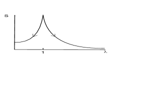
Figure 4: This figure is based on results of crit2 . It shows the dependence of the entanglement entropy in the Ising spin chain (6) at a fixed $N$ as a function of magnetic field strength $\lambda$. The critical point $\lambda=1$ is ultaviolet fixed point. The arrows show directions of the RG flow from the ultraviolet to infrared regions.

The RG-evolution of the entanglement entropy for the Ising model is known precisely crit2 . The dependence of the entanglement entropy in the Ising spin chain (6) at a fixed $N$ as a function of magnetic field strength $\lambda$ is shown on Fig. 4. This behaviour is in accord with a general property: in unitary theories the entanglement entropy should not increase along the RG flow because RG transformations eliminate contribution of the high energy modes.

The fact that the entropy is not increasing does not imply the same property for the induced coupling $G^{-1}$ defined by (57). The coupling behaves as the density of the entropy, $G^{-1}(t)=t^{D-2}f(t)$, where $D$ is the number of space-time dimensions and $f(t)$ is a function which has the same RG-evolution as the entropy. In three-dimensional model discussed in Section II.D the induced gravitational coupling defined by (57) increases under RG-evolution. On the other hand, in four-dimensional model the gravitational coupling decreases which means that gravitational interactions get weaker in the infrared region.

IV.2 The scaling hypothesis

The scaling hypothesis in classical critical phenomena asserts that the physics is determined by large scale fluctuations which do not depend on the underlying microscopical details. For instance, in a magnetic at temperature $T$ in an external field $h$ which undergoes a second order phase transition the physical properties are determined by the large domains of aligned spins. The microscopic atomic scale does not enter thermodynamical relations near the critical point $T=T_{c}$. Non-analytic dependence of the physical quantities on $|T-T_{c}|$ is entirely determined by a ”singular part” of free energy density $f_{\mbox{\tiny{sing}}}$. This part has a universal scaling

$$f_{\mbox{\tiny{sing}}}(t,h)=\xi^{-(D-1)}f_{\pm}(h\xi^{-d_{h}})~{}~{}~{},$$

where $\xi\sim|T-T_{c}|^{-\nu}$ is the correlation length and $d_{h}$ is the scaling dimension of $h$. Functions $f_{\pm}$ are universal in a sense they coincide for different systems from the same class.

Let us denote by ${\cal S}_{\mbox{\tiny{ren}}}$ the surface density of the ”renormalized” part of the entanglement entropy in the ground state, see Section II.E. This is the part of the entropy which remains finite in the limit $\varrho=0$. In general, ${\cal S}_{\mbox{\tiny{ren}}}$ is a function of external fields $h$, and other parameters, $g$, driving the phase transition of the system at $g=g_{c}$. By using analogy with the classical scaling one can conjecture that near a critical point ${\cal S}_{\mbox{\tiny{ren}}}$ has the following scaling

$${\cal S}_{\mbox{\tiny{ren}}}(g,h)=\xi^{-(D-2)}s_{\pm}(h\xi^{-d_{h}})~{}~{}~{},$$ (59)

where $\xi=|g-g_{c}|^{-\nu}$ is the correlation length, $d_{h}$ is the scaling dimension, and $s_{\pm}$ are universal functions. It can be also suggested that the divergent part of the entropy is analytic in $g$.

One can check the validity of these statements in scalar field models discussed in Section II.D. In the limit when the edge size $L$ of the cube is large one finds from (35), (37) that $s_{\pm}=-1/(24)$ in $D=3$ and $s_{\pm}=-1/(24\pi)\ln(m/\mu)$ in $D=4$.

In analogue models of gravity the universality conjecture (59) means that the part of the induced Newton coupling (57) which does not depend on the cutoff is a universal function. This part of the coupling can be determined entirely in terms of an effective low-energy QFT and it does not depend on the details of the underlying microscopic theory.

IV.3 The problem of black hole entropy

Studying entanglement in gravity analogs might be helpful for understanding the microscopical origin of the Bekenstein-Hawking entropy $S^{BH}$ of black holes. As was discussed in Section I.B, if the gravity is entirely induced by some underlying degrees of freedom the entropy of a black hole can be related to the entanglement between observable states and states hidden inside the horizon. Understanding the relation between the two entropies in the framework of a local relativistic quantum field theory is plagued by the problem of the ultraviolet divergences. The definition of the induced Newton coupling either requires introduction of the ultraviolet cutoff or working with a special class of ultraviolet finite theories with non-minimal couplings FFZ:96 , FF:97 . The presence of non-minimal couplings makes statistical interpretation of $S^{BH}$ a difficult task.

The equality of $S^{BH}$ to the fundamental entanglement entropy $S$ is implied in suggestion (4). One of the arguments why it should be true is that both in classical and in quantum theory the Bekenstein-Hawking entropy can be derived by the conical singularity method from the gravitational action (see e.g. FrFu:98 , FS1 ), in the same way which we employed for calculation of $S$.

If equality (4) holds one has a tool to learn more about the degrees of freedom responsible for the origin of $S^{BH}$ by using gravity analogs. There are different questions which can be addressed in different models. For instance, can one relate these degrees of freedom in the 3D Ising model with non-critical stings, do the near-horizon symmetries play any role in the entropy counting as was suggested in Carlip:05 , and other questions.

V Summary

This paper has two purposes. First, we wanted to show how the effective action approach and the methods of spectral geometry can be applied for derivation of the entanglement entropy in condensed matter systems in the regimes when these systems can be described by relativistic QFT’s. In particular, such regimes appear in the vicinity of the second order phase transitions. By using the effective action approach we established the form of the entanglement entropy in the presence of boundaries at zero and high temperatures. Our new result is establishing the geometrical structure of the subleading terms in the entropy, Eq. (5).

Second, we showed that in the effective action approach the black hole entropy and the entanglement entropy have the same geometrical origin, the conical singularities of a background manifold. On this base we conjectured (and this is the main result of the paper) that the surface density of the fundamental entanglement entropy in the genuine quantum gravity theory and the low-energy gravitational coupling $G_{N}$ are related by (4). Finally, we suggested to use this relation to study the properties of $G_{N}$ in analogue gravity models and pointed several topics where this kind of research could be interesting.

References

- (1) J. Preskill, J. Mod. Opt. 47 (2000) 127, quant-ph/9904022.
- (2) M. Srednicki, Phys. Rev. Lett. 71 (1993) 666, hep-th/9303048.
- (3) L. Bombelli, R.K. Koul, J. Lee and R.D. Sorkin, Phys. Rev. D34 (1986) 373.
- (4) M.B. Plenio, J. Eisert, J. Dreissig and M. Cramer, Phys. Rev. Lett. 94 (2005) 060503.
- (5) M.B. Plenio, J. Eisert, J. Dreissig and M. Cramer, Phys. Rev. A73 (2006) 012309.
- (6) W. Israel, Phys. Lett. 57A (1976) 107.
- (7) V. Frolov and D. Fursaev, Class. Quantum Grav. 15 (1998) 2041.
- (8) L. Susskind and J. Uglum, Phys. Rev. D50 (1994) 2700.
- (9) C. Callan and F. Wilczek, Phys. Lett B333 (1994) 55.
- (10) A.D. Sakharov, Sov. Phys. Dokl. 12 (1968) 1040.
- (11) T. Jacobson, Black Hole Entropy in Induced Gravity, gr-qc/9404039.
- (12) V.P. Frolov, D.V. Fursaev, A.I. Zelnikov, Nucl. Phys. B486 (1997) 339, hep-th/9607104.
- (13) V.P. Frolov, D.V. Fursaev, Phys. Rev. D56 (1997) 2212, hep-th/9703178.
- (14) S.W. Hawking, J.M. Maldacena, A. Strominger, JHEP 0105 (2001) 001, hep-th/0002145.
- (15) J.M. Maldacena, JHEP 04 (2003) 021, hep-th/0106112.
- (16) R. Burstein, M.B. Einhorn, A. Yarom, Entanglement Interpretation of Black Hole Entropy in String Theory, hep-th/0508217.
- (17) G. Vidal, J.I. Latorre, E. Rico, A. Kitaev, Phys. Rev. Lett. 90 (2003) 227902, quant-ph/0211074.
- (18) J.I. Latorre, E. Rico and G. Vidal, Quant. Inf. and Comp. 4 (1) (2004) 048, quant-ph/0304098.
- (19) J.I. Latorre, R.Orus, E. Rico and J. Vidal, Entanglement Entropy in the Lipkin-Meshkov-Glick Model, cond-amt/0409611.
- (20) E. Rico, Quantum Correlations in (1+1)-dimensional systems, Ph.D. Thesis, quant-ph/0509037.
- (21) D.V. Fursaev and S.N. Solodukhin, Phys. Rev. D52 (1995) 2133.
- (22) D.V. Vassilevich, Phys. Rep. 388 (2003) 279.
- (23) D.V. Fursaev, Phys. Lett. B334 (1994) 53.
- (24) P. Calabrese and J. Cardy, JSTAT 0406 (2004) P002, hep-th/0405152.
- (25) A. Kitaev and J.Preskill, Topological entanglement entropy, hep-th/0510092.
- (26) D. Gioev, I. Klich, quant-ph/0504151.
- (27) M.M. Wolf, Entropic Area law for Fermions, quant-ph/0503219.
- (28) T. Barthel, M.-C. Chung, U. Schollwoeck,Entanglement Scaling in Critical Two-dimensional Fermionic and Bosonic Systems, cond-mat/0602077.
- (29) J.S. Dowker and J.P. Schofield, J. Math. Phys. 31 (1990) 808.
- (30) C. Holzey, F. Larsen, and F. Wilczek, Nucl. Phys. B424 (1994) 44, hep-th/940308.
- (31) J.S. Dowker and J.P. Schofield, Phys. Rev. D38 (1988) 3327.
- (32) D.V. Fursaev and S.N. Solodukhin, Phys. Lett. B365 (1996) 51.
- (33) A.M. Polyakov, Phys. Lett. 82B (1979) 247; A.M. Polyakov, Gauge Fields and Strings, Harwood Academic Publishers, 1987.
- (34) W.G. Unruh, Phys. Rev. Lett. 46 (1981) 1351.
- (35) G.E. Volovik, Universe in a Helium Droplet, Oxford University Press, Oxford, 2003; C. Barcelo, S. Liberati, M. Visser, Analogue Gravity, gr-qc/0505065.
- (36) J.I. Latorre, C.A. Lütken, E. Rico, G. Vidal, Phys. Rev. A71 (2005) 034301, quant-ph/0404120.
- (37) S. Carlip, Class. Quantum Grav. 22 (2005) 3055, gr-qc/0501033.