Zero modes on cosmic strings in an external magnetic field

Abstract

A classical analysis suggests that an external magnetic field can cause trajectories of charge carriers on a superconducting domain wall or cosmic string to bend, thus expelling charge carriers with energy above the mass threshold into the bulk. We study this process by solving the Dirac equation for a fermion of mass $m_{f}$ and charge $e$, in the background of a domain wall and a magnetic field of strength $B$. We find that the modes of the charge carriers get shifted into the bulk, in agreement with classical expectations. However the dispersion relation for the zero modes changes dramatically — instead of the usual linear dispersion relation, $\omega_{k}=k$, the new dispersion relation is well fit by $\omega\approx m_{f}~{}{\rm tanh}(k/k_{*})$ where $k_{*}=m_{f}$ for a thin wall in the weak field limit, and $k_{*}=eBw$ for a thick wall of width $w$. This result shows that the energy of the charge carriers on the domain wall remains below the threshold for expulsion even in the presence of an external magnetic field. If charge carriers are expelled due to an additional perturbation, they are most likely to be ejected at the threshold energy $\sim m_{f}$.

I Introduction

Fermion zero modes on domain walls and cosmic strings have been known to exist since the 60’s Caroli:1964 ; Jackiw:1981ee . If the fermions are electrically charged, it is generally presumed that the string or wall is superconducting in the sense that it can sustain long-lived persistent currents Witten:1984eb . Such superconducting strings could be present in the universe, and would have observable electromagnetic and other signatures (for a review, see VilShe ). Light superconducting strings could also be trapped in the center of our galaxy and could explain Ferrer:2005xv the observed positron annihilation line SPI .

The observable signatures of cosmic superconducting strings depend on the magnitude of the currents they carry. As the strings move under their tension, they cut across ambient astrophysical magnetic fields and this generates currents on the strings. Interactions of charge carriers on the string are expected to limit the maximum current that a string can carry Barr:1987ij . Hence it is important to understand the interaction of a superconducting string with an external magnetic field.

In this paper we consider a straight, static, current-carrying, string, placed in a background magnetic field. The magnetic field is assumed to be perpendicular to the string. The charge carriers on the string feel the background magnetic field via the Lorentz force which is also perpendicular to the string. Thus the ambient magnetic field tends to bend the charge carriers off the string as depicted in Fig. 1.

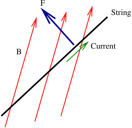
Figure 1: The charge carriers run along the string. In the presence of a perpendicular external magnetic field, the Lorentz force would tend to bend the charges off the string.

The dispersion relation for zero modes on a string (with no external magnetic field) is that for a massless particle

$$\omega_{k}=+k$$ (1)

where, to be specific, we have taken the $+$ sign. (If the zero mode propagates in the opposite direction along the string, we would have $\omega_{k}=-k$.) The dispersion relation for the remaining (“non-zero”) modes is of the form

$$\omega_{k}=\pm\sqrt{{\bf k}^{2}+m^{2}}$$ (2)

where $m$ is a mass associated with the mode. For scattering states, $m$ is the mass of the fermion in vacuum, $m_{f}$. For a particle in a zero mode state to escape, it has to transition into a scattering state. Since a particle in a zero mode only has kinetic energy, to escape into the bulk, its kinetic energy has to transform into mass energy. For $k>m_{f}$, this is not forbidden by energy conservation because it is possible to find the scattered momentum, ${\bf k}^{\prime}$, such that $|k|=\sqrt{{{\bf k}}^{\prime 2}+m_{f}^{2}}$.

Let us consider a particle in a zero mode with $k/m\rightarrow\infty$. The particle certainly has enough energy to escape the string. The question is whether an external magnetic field can trigger this escape. At first sight it would appear that the fermion zero mode is very fragile since it is a bound state as regards its motion perpendicular to the string, yet it is degenerate with continuum states that are unbound. Such bound states are known to dissolve resonantly into the the continuum under the effect of even a very weak perturbation, for example, in the auto-ionization of excited atomic Helium. However, as shown by Fano Fano , in order to destroy a bound state a perturbation must couple it to continuum states with which it is degenerate. Due to the translational symmetry of the problem it is easy to see that a uniform magnetic field does not couple the zero mode to continuum states that are degenerate with it. One way to understand this result is to note that all the energy of the zero mode is kinetic energy, while only a fraction of the particle energy off the string is kinetic. To be ejected from the string, some of the kinetic energy of the zero mode has to get converted into mass energy, and the magnitude of the momentum of the particle off the string therefore has to be less than that of the zero mode. Thus we are lead to the conclusion that at least perturbatively a uniform magnetic field does not destroy the zero mode by Fano’s mechanism. It is therefore necessary to analyse the effect of the magnetic field non-perturbatively in order to definitively settle the question. In this paper we carry out such a non-perturbative analysis.

For the reader who may not wish to go through all the details, we briefly summarize our result for the dispersion relation for fermions on a string or domain wall in the presence of a magnetic field. The dispersion relation for small wavevectors, $k$, resembles that of a zero mode on a string without any magnetic field. Intuitively, $k$ is the momentum of the particle and at zero momentum, there is no Lorentz force and so the magnetic field plays no role. Hence the dispersion relation is linear for small $k$. On the other hand, at large $k$, the magnetic field dominates and the dispersion relation is as if there is no domain wall. In this regime, the energy is independent of $k$, just as in the Landau problem. The transition of the dispersion from linear in $k$ to independent of $k$ occurs when the effect of the domain wall is comparable to that of the external magnetic field, or approximately at $k_{*}$ where $k_{*}=m_{f}$ for a thin wall in the weak field limit, and $k_{*}=eBw$ for a thick wall of width $w$. Thus the fermions in the lowest energy level have a dispersion relation that is of the form

$$\omega_{k}=m_{f}{\rm tanh}\biggl{(}\frac{k}{k_{*}}\biggr{)}$$ (3)

This dispersion is exact in the thick wall limit and fits our numerical results reasonably well in other cases.

The modified form of the dispersion relation for superconducting strings may be important in astrophysical applications as briefly described in the concluding section.

II Simplifying the problem

The proper framework for discussing the effect of external magnetic fields on zero modes on strings is in terms of the field theory of scalar and gauge fields that gives a string solution, the fermions which have zero modes on the string, and the external magnetic field. Such a model is quite complicated and it is desirable to find a simpler model with all the relevant physics. For this reason we consider a field theory in two spatial dimensions that has domain wall solutions, a fermion with zero modes on the domain wall, and a magnetic field. The Lagrangian for the model containing a scalar field, $\phi$, a fermion, $\psi$, and a vector field, $A_{\mu}$, is

$$L = \frac{1}{2}(\partial_{\mu}\phi)^{2}+\frac{m^{2}}{2}\phi^{2}-\frac{\lambda}{4}\phi^{4}-\frac{1}{4}F_{\mu\nu}F^{\mu\nu}$$ (4)

$$+ i{\bar{\psi}}\gamma^{\mu}(\partial_{\mu}+ieA_{\mu})\psi-g\phi{\bar{\psi}}\psi$$

The $\gamma$ matrices are defined, in terms of the Pauli spin matrices, by

$$\gamma^{t}=\sigma_{3}\ ,\ \ \gamma^{x}=i\sigma_{2}\ ,\ \ \gamma^{y}=-i\sigma_{1}$$ (5)

The scalar sector of the field theory is the $\lambda\phi^{4}$ model and has the classical domain wall solution

$$\phi(x)=\eta{\rm tanh}\left(\frac{x}{w}\right)$$ (6)

where $\eta=m/\sqrt{\lambda}$ and $w=\sqrt{2}/m$ is the width of the wall.

In the absence of an external magnetic field, the fermionic zero mode is

$$\psi_{0}(x)=N\left[{\rm sech}\left(\frac{x}{w}\right)\right]^{g\eta w}\left(\begin{array}[]{c}1\\ i\end{array}\right)$$ (7)

This solution has zero momentum and zero energy. It can be boosted along the direction of the wall to get a propagating zero mode

$$\psi_{k}(t,x,y)=\exp\left[{-i(\omega t-ky)}\right]\psi_{0}(x)$$ (8)

The dispersion relation is as in Eq. (1)

$$\omega^{0}_{k}=+k$$ (9)

In Sec. IV we will discuss the zero modes when we also have an external magnetic field. To gain intuition for the final results, we now discuss the Landau problem of fermions in a magnetic field but without a domain wall.

III Relativistic Landau problem

We now consider the fermion modes in a magnetic field taken to be uniform in the $xy-$plane. The potential is

$$A^{\mu}=\left(0,0,-Bx\right)\ ,\ \ \mu=t,x,y$$ (10)

With this choice of gauge, the fermion wavefunctions can be factorized as in Eq. (8) and we can solve for the functions $\psi^{B}$.

There is a special eigenmode with $\omega_{0,k}^{B}=-m_{f}$

$$\psi^{B}_{0,k}=\left(\begin{array}[]{c}0\\ \varphi_{0}\left(x+x_{0}\right)\end{array}\right)e^{-i(\omega^{B}_{0,k}t-ky)}$$ (11)

where

$$x_{0}=\frac{k}{eB}$$ (12)

The remaining relativistic Landau eigenfunctions are

$$\psi^{B}_{n,k\pm} = A_{n,\pm}\left(\begin{array}[]{c}\varphi_{n}\left(x+x_{0}\right)\\ \\ \frac{i\sqrt{2eB(n+1)}}{m_{f}\pm\sqrt{m_{f}^{2}+2eB(n+1)}}\varphi_{n+1}\left(x+x_{0}\right)\end{array}\right)$$ (17)

$$\hskip 72.26999pt\times e^{-i(\omega^{B}_{n,k,\pm}t-ky)}$$

with energy eigenvalues

$$\omega^{B}_{n,k,\pm}=\pm\sqrt{m_{f}^{2}+2eB(n+1)},\quad n=0,1,2,\ldots$$ (18)

Note that the energy eigenvalues in the Landau problem are independent of the wavevector $k$.

Here $A_{n,\pm}$ are normalization constants and $\varphi_{n}(x)$ is the solution to the shifted harmonic oscillator equation which can be expressed in terms of Hermite polynomials:

$$\varphi_{n}(x)=\frac{(eB)^{1/4}}{\pi^{1/4}2^{n/2}n!}H_{n}\left(x\sqrt{eB}\right)\exp\left(\frac{-eBx^{2}}{2}\right)$$ (19)

IV Domain wall in a magnetic field

Now we consider the full setting where there is a domain wall along the $y-$axis, and a uniform magnetic field of magnitude $B$ in the $xy-$plane (see Fig. 2). Then the scalar field is as given in Eq. (6) and the gauge field in Eq. (10).

Figure 2: In our simplified setup, a domain wall lies along the $y-$axis and a uniform magnetic field lies in the $xy-$plane. Fermion zero modes run along the wall i.e. in the $y-$direction.

The Dirac equation now reads

$$\left(i\gamma^{\mu}\partial_{\mu}+eBx\gamma^{2}-g\phi(x)\right)\psi=0$$ (20)

This is the equation for a Dirac particle moving in a uniform magnetic field with a position dependent mass $m(x)=g\phi(x)$. Far from the wall, the mass approaches the asymptotic value $\pm m_{f}$ as $x\rightarrow\pm\infty$, where $m_{f}=g\eta$

To find the eigenstates of Eq. (20), we write

$$\psi(t,x,y)=\pmatrix{\chi_{1}(x)\cr\chi_{2}(x)}e^{-i(\omega t-ky)}$$ (21)

The equation for the $\chi$ fields is

$$\left(\begin{array}[]{cc}m(x)-\omega&-i\partial_{x}-ik-ieBx\\ -i\partial_{x}+ik+ieBx&-m(x)-\omega\end{array}\right)\left(\begin{array}[]{c}\chi_{1}\\ \chi_{2}\end{array}\right)=0$$ (22)

The dimensionful scales that characterize the system are: $w$, $m_{f}$, and $eB$, with $w$ and $m_{f}$ both occurring within $m(x)$. These dimensionful parameters can be written as three length scales in the problem: $w$, $l_{\psi}\equiv m_{f}^{-1}$ and $l_{B}\equiv 1/\sqrt{eB}$. In addition, a mode is characterized by its wavelength $2\pi/k$. Only the ratio of the various length scales is important. For convenience, we work in units where $w=1$ except in the thin wall approximation (Sec. IV.4) where we take $w\rightarrow 0$.

We would like to find all solutions to Eq. (22). This is possible to do analytically in two extreme limits (1) thick domain wall ($w\gg l_{\psi},\>l_{B}$), and (2) thin domain wall ($w\ll l_{\psi},\>l_{B}$). In general, the modes need to be found numerically. Before discussing the solutions, it is necessary to clarify the concept of a zero mode in the presence of a magnetic field and to prove that such a mode does exist in general and not only in the two limiting cases for which we can find exact solutions.

IV.1 Zero mode at $k=0$

At zero magnetic field, the key distinguishing features of the zero mode state are that it is localised in a direction perpendicular to the domain wall (along the $x$-axis) and has zero energy at $k=0$. With a magnetic field turned on, in the present gauge, all wavefunctions are localised along the $x$-direction, but we can still ask whether there is a zero energy state and, if so, identify it as the magnetic field analog of the zero-mode state. To this end, we must study Eq. (22) and ask whether it has well-behaved solutions with $\omega=0$ when we set $k=0$.

In the zero field case studied in section II, we were able to establish the existence of the zero mode by explicit, exact solution of the Dirac equation. This is a rare luxury; under more typical circumstances it is necessary to resort to index theorems eweinberg or other indirect arguments to establish the existence of zero modes. The strategy we follow here is to eliminate $\chi_{2}$ and rewrite Eq. (22) as a second-order equation

$$-\frac{\partial^{2}}{\partial x^{2}}\chi_{1}+\frac{m^{\prime}}{m}\frac{\partial}{\partial x}\chi_{1}+$$

$$\left(m^{2}+eB+e^{2}B^{2}x^{2}-\frac{m^{\prime}}{m}eBx\right)\chi_{1}=0,$$ (23)

where $m\equiv m(x)$ and $m^{\prime}\equiv\partial m/\partial x$. Once this equation has been solved for $\chi_{1}$ we may determine $\chi_{2}$ via

$$\chi_{2}=-\frac{i}{m}\frac{\partial}{\partial x}\chi_{1}+i\frac{eB}{m}x\chi_{1}$$ (24)

For $x\rightarrow\infty$ we may set $m^{\prime}=0$ in Eq. (23) and thereby find that in this asymptotic region $\chi_{1}$ obeys the Schrödinger equation of a non-relativistic oscillator. Therefore it has one solution that grows as $x\rightarrow\infty$ and one that is well-behaved and decays. The key question now is whether a well-behaved solution can be found at $x=0$ that will connect with the well-behaved solution at $+\infty$. Since $m(x)=0$ for $x=0$, it is clear that the origin is a (regular) singular point for the differential equation (23) and it appears to be a possibility that of the two independent solutions near the origin only one is regular. However, by use of a series expansion, we can show that there are in fact two independent solutions that are both regular at $x=0$. One has the series expansion

$$\chi_{1}=1+\frac{1}{8}\left(\mu_{1}^{2}-2\frac{\mu_{3}}{\mu_{1}}eB+e^{2}B^{2}\right)x^{4}+\ldots;$$ (25)

the other has the expansion

$$\chi_{1}=x^{2}+\frac{\mu_{3}}{2\mu_{1}}x^{4}+\ldots$$ (26)

Here we have taken $m(x)=\mu_{1}x+\mu_{3}x^{3}+\ldots$ near the origin. A generic combination of these two solutions would develop into a superposition of the growing and decaying solutions as $x\rightarrow\infty$; but by fine-tuning the coefficients we can arrange for the solution to decay as $x\rightarrow\infty$. Furthermore, since the solutions in Eqs. (25) and (26) are both even, and the differential Eq. (23) is also even, it follows that the solution will be even and well-behaved as $x\rightarrow-\infty$ as well. This concludes our demonstration that there is a zero energy solution to Eq. (22) for $k=0$.

IV.2 Zero mode for non-zero $k$

We turn now to the magnetic zero mode for non-zero $k$. It is shown below that for a fixed $k$ Eq. (22) has a discrete spectrum of eigenvalues $\omega$. Thus we may hope to identify the zero mode at non-zero $k$ as the state that smoothly evolves into the zero energy state as $k\rightarrow 0$. That such a state exists is not obvious: there is a competing possibility that the spectrum is not continuous as $k\rightarrow 0$ and that the zero energy state at $k=0$ has no counterpart for non-zero $k$. In this section, however, we will give a variational argument that makes it certain beyond reasonable doubt that the spectrum is continuous at $k=0$ and that the zero mode therefore continues to exist for non-zero $k$. Further, we are able to verify this continuity and to study the evolution of the zero mode with $k$ explicitly in the thick and thin wall limits discussed in the subsections below.

To study the magnetic zero mode for non-zero $k$ it is helpful to rewrite Eq. (22) as a second-order equation by analogy to Eq. (23). We obtain

$$\frac{\partial^{2}}{\partial x^{2}}\chi_{1} - \frac{m^{\prime}}{(\omega+m)}\frac{\partial}{\partial x}\chi_{1}+\left[\omega^{2}-m^{2}-eB-(k+eBx)^{2}\right.$$ (27)

$$+ \left.\frac{m^{\prime}}{(\omega+m)}(k+eBx)\right]\chi_{1}=0$$

where we have used

$$\chi_{2}=-\frac{i}{(\omega+m)}\frac{\partial}{\partial x}\chi_{1}+\frac{ieBx}{(\omega+m)}\chi_{1}+ik\chi_{1}$$ (28)

to eliminate $\chi_{2}$ from the coupled Eq. (22). As $x\rightarrow\pm\infty$ we may set $m^{\prime}=0$ and find that Eq. (27) turns into the equation of a non-relativistic oscillator. Therefore it has a discrete spectrum.

For $\omega$ outside the mass gap ($\omega>m_{f}$ or $\omega<-m_{f}$) Eq. (27) is not singular on the real axis. Thus for any $\omega$ we can find a solution that is well behaved at the origin and as $x\rightarrow\infty$. By tuning $\omega$ to a quantised energy level we can also ensure that it is well behaved as $x\rightarrow-\infty$. Thus it is easy to see that a discrete spectrum will arise outside the mass gap. However for the present purpose these states are of no interest since they will not continuously evolve into the zero energy state as $k\rightarrow 0$.

If we look for states that lie below the mass gap ($-m_{f}<\omega<m_{f}$) we must come to grips with the fact that Eq. (27) is singular at $x_{0}$ where $x_{0}$ is fixed by the condition $\omega+m(x_{0})=0$. By making a series expansion about this point it is easy to show that Eq. (27) has one well behaved solution at this point and one that is singular. Thus we must fine-tune $\omega$ in order to obtain a solution that behaves well as $x\rightarrow\infty$. Since Eq. (27) is not symmetric about $x_{0}$, it is not obvious that the solution will be well behaved as $x\rightarrow-\infty$. This raises the real concern that there may be no eigenstates within the mass gap for non-zero $k$ and therefore no continuation of the $k=0$ state of zero energy.

To put this concern to rest and to establish that there are in fact states within the mass gap we turn to a variational argument. To this end, it is convenient to write Eq. (22) in the form

$$H\left(\begin{array}[]{c}\chi_{1}\\ \chi_{2}\end{array}\right)=\omega\left(\begin{array}[]{c}\chi_{1}\\ \chi_{2}\end{array}\right).$$ (29)

Here $H$ is an hermitean matrix differential operator and we regard $k$ as a fixed parameter. Now $H^{2}$ has a spectrum that is bounded from below and it is therefore an operator to which the variational principle may be applied. We will seek a normalised state $|\Omega\rangle$ that satisfies $\langle\Omega|H^{2}|\Omega\rangle<m_{f}^{2}$. This implies that $H^{2}$ has an eigenvalue below $m_{f}^{2}$ for every value of $k$, and in turn that $H$ has an eigenvalue within the mass gap.

For the state $|\Omega\rangle$ we take

$$\left(\begin{array}[]{c}\chi_{1}\\ \chi_{2}\end{array}\right)=\frac{1}{\sqrt{2}}\left(\begin{array}[]{c}\exp(-|x|)\\ i\exp(-|x|)\end{array}\right).$$ (30)

A straightforward computation reveals

$$\frac{1}{m_{f}^{2}}\langle\Omega|H^{2}|\Omega\rangle = 3-4\ln 2-\frac{4}{m_{f}}\left(\ln 2-\frac{1}{2}\right)$$ (31)

$$+\frac{1}{m_{f}^{2}}\left(1+k^{2}+\frac{1}{2}e^{2}B^{2}\right).$$

We would like to ensure that the right hand side of Eq. (31) is less than unity. For suitable parameters this is clearly the case. Thus at least over a certain range of $m_{f}$ and $eB$ there are sub-gap states for small non-zero $k$. By continuity we may therefore reasonably conclude that quite generally there is a state that is the continuation to non-zero $k$ of the zero energy state at $k=0$. We will confirm this expectation by approximate solution to the problem in the thick wall limit and exact solution in the thin wall limit below.

IV.3 Thick wall

In the limit that the wall thickness is large it is possible to derive asymptotic expressions for the zero mode as well as the lowest few excited states that lie outside the mass gap. To understand the approximation involved it is instructive to set $m^{\prime}\rightarrow 0$ in Eq. (27). On doing so we see that $\chi_{1}$ obeys the Schrödinger equation for a harmonic oscillator centered at $x_{0}=-k/eB$. The width of the oscillator wave function is $1/\sqrt{eB}$. Since we are working in units where the wall width $w=1$, it would appear that the approximation of treating $m(x)$ as constant and equal to $m(x_{0})$ should be accurate when the extent of the wavefunctions is small compared to the distance over which the mass varies, i.e., in the high field regime $1/(eB)\ll 1$. In Appendix A we will show that the condition for validity is slightly more restrictive.

In summary the thick wall approximation consists of replacing $m(x)$ in Eq. (22) with the constant $m(x_{0})$ where $x_{0}=-k/(eB)$. The solution to Eq. (22) in this approximation may then be read off from the solution to the relativistic Landau problem given in section III. Proceeding in this way, we find that the zero mode state that lies within the mass gap has an energy

$$\omega_{B}^{0}(k)=-m(x_{0})=m_{f}\tanh\left(\frac{k}{eB}\right)$$ (32)

and a wavefunction given by Eqs. (11) and (19).

There are several noteworthy features of this zero-mode solution. First observe that indeed $\omega_{B}^{0}\rightarrow 0$ as $k\rightarrow 0$, showing that this state is continuous with the zero energy state at $k=0$. Hence this state is identifiable as the zero mode state for non-zero $k$. Next we see that in contrast to the situation at zero magnetic field, the dispersion relation of the zero mode is linear only for small $k$. For larger $k$, $\omega_{B}^{0}$ saturates and always remains within the mass gap even as $k\rightarrow\pm\infty$. At zero field the zero mode wave function is always localised about the domain wall; indeed it is independent of $k$ in this case. By contrast with a magnetic field the zero mode wavefunction is centered about $x_{0}=-k/(eB)$ and it moves far away from the domain wall as $k\rightarrow\pm\infty$. The shape of the wavefunction is always a Gaussian and does not depend on $k$.

Evidently in the thick wall limit the low lying excited states of Eq. (22) are also given by Eqs. (18), and (19) if we substitute $m\rightarrow m(x_{0})=-m_{f}\tanh(k/eB)$. For sufficiently excited states this approximation will break down because the width of the wavefunctions grows to a point that it is no longer appropriate to treat $m(x)$ as a constant equal to its value at the center of the wavefunction.

To conclude we give the conditions for validity of the thick wall approximation to the zero mode. It is shown in Appendix A that the approximate solution is good if $eB\gg 1$ and either $|x_{0}|=|k/eB|\gg 1$ or $m_{f}\ll eB$. Here, as elsewhere in this subsection, we have worked in units where the wall width $w=1$.

IV.4 Thin wall

In this approximation the wall profile corresponds to a sharp step

$$m(x)=m_{f}\Theta(x)-m_{f}\Theta(-x)$$ (33)

With this profile Eq. (27) leads to the following second order equation for $\chi_{1}$

$$\frac{\partial^{2}\chi_{1}}{\partial x^{2}}+\left[\omega^{2}-m_{f}^{2}-eB-(k+eBx)^{2}\right]\chi_{1}=0\ ,\ \ x\neq 0$$ (34)

This is the equation of a shifted harmonic oscillator. With the change of variables $z=\sqrt{2eB}\left(x+x_{0}\right)$, where $x_{0}=k/eB$, Eq. (34) takes the form of Weber’s equation whittaker :

$$\frac{\partial^{2}\chi_{1}}{\partial z^{2}}+\left[\nu+\frac{1}{2}-\frac{z^{2}}{4}\right]\chi_{1}=0$$ (35)

Here

$$\nu=\frac{\omega^{2}-m_{f}^{2}}{2eB}-1$$ (36)

is not generally an integer.

A well-behaved, i.e. tending to 0 as $x\rightarrow\pm\infty$, solution to Eq. (35) can be given in terms of the Weber function

$$\chi_{1}(x)=\left\{\begin{array}[]{l c}D_{\nu}\left(\sqrt{2eB}\left(x+x_{0}\right)\right),&x>0\\ CD_{\nu}\left(-\sqrt{2eB}\left(x+x_{0}\right)\right),&x<0\end{array}\right.$$ (37)

where $\nu$ is given in Eq. (36) and

$$C=\frac{D_{\nu}\left(x_{0}\sqrt{2eB}\right)}{D_{\nu}\left(-x_{0}\sqrt{2eB}\right)}$$ (38)

is found by demanding continuity of the wavefunction at the origin. Note that the derivative $\partial_{x}\chi_{1}$ will be discontinuous at $x=0$ due to the non smooth wall profile there. The quantization of $\nu$ in Eq. (36) arises in the simple harmonic oscillator problem in quantum mechanics from imposing that $\partial_{x}\chi_{1}$ be continuous, but in the problem at hand, the energy will only be determined after requiring continuity of the lower component, $\chi_{2}$, of the eigenmodes

$$\chi_{2}(x)=\left\{\begin{array}[]{l c}\frac{-i}{\omega+m_{f}}\left[\partial_{x}\chi_{1}-(k+eBx)\chi_{1}\right],&x>0\\ &\\ \frac{-i}{\omega-m_{f}}\left[\partial_{x}\chi_{1}-(k+eBx)\chi_{1}\right],&x<0\end{array}\right.$$ (39)

This can also be expressed in terms of Weber functions

$$\chi_{2}(x)=\left\{\begin{array}[]{l c}\frac{-i}{\omega+m_{f}}\left[\sqrt{2eB}\nu D_{\nu-1}-2(k+eBx)D_{\nu}\right],&x>0\\ &\\ \frac{-iC}{\omega-m_{f}}\left[-\sqrt{2eB}\nu D_{\nu-1}-2(k+eBx)D_{\nu}\right],&x<0\end{array}\right.$$ (40)

where $C$ is also given by Eq. (38).

Requiring that $\chi_{2}$ be continuous leads to the quantization relation that determines the possible energies of the eigenmodes:

$$4km_{f}D_{\nu}\left(-k\sqrt{2/eB}\right)D_{\nu}\left(k\sqrt{2/eB}\right)=-\sqrt{2eB}\nu$$

$$\times\left[(\omega+m)D_{\nu-1}\left(-k\sqrt{2/eB}\right)D_{\nu}\left(k\sqrt{2/eB}\right)\right.$$

$$+\left.(\omega-m)D_{\nu-1}\left(k\sqrt{2/eB}\right)D_{\nu}\left(-k\sqrt{2/eB}\right)\right]$$ (41)

where $\nu$ is given in Eq. (36).

In order to numerically solve the condition in Eq. (41), it is convenient to express the Weber functions in terms of hypergeometric functions. This is done in Appendix B, In Fig. 3 we show the shape of the dispersion relation for the zero modes for $eB=m_{f}=1$ and a few of the scattering states.

The numerical results from Eq. (41) can be approximately fit by Eq. (3). Indeed, using the results in Appendix B, we can study the dispersion relation around the origin, $k=0$, to find $k_{*}$:

$$\frac{m_{f}}{k_{*}}=\left.\frac{d\omega}{dk}\right|_{k=0}=2^{1-v^{2}}\sqrt{\frac{\pi}{2}}\>v\>\Gamma\left(2+v^{2}\right)\times$$

$$\left[\frac{1}{\left(1+v^{2}\right)\Gamma\left(1+\frac{v^{2}}{2}\right)}-\frac{1}{\Gamma\left(1+\frac{v^{2}}{2}\right)^{2}}+\right.$$

$$\left.\frac{1}{\Gamma\left(\frac{1}{2}+\frac{v^{2}}{2}\right)\Gamma\left(\frac{3}{2}+\frac{v^{2}}{2}\right)}\right],$$ (42)

where $v\equiv m_{f}/\sqrt{2eB}$. The absolute value of the slope $d\omega/dk$ at the origin is always less than $1$, approaching this value asymptotically for large values of $|v|$, i.e. for small magnetic fields.

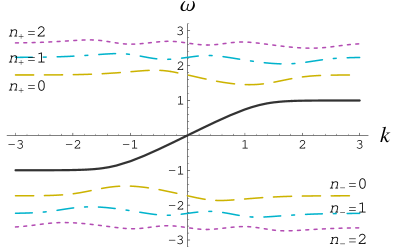
Figure 3: Dispersion relation for the zero modes and the lowest few excited states that lie outside the mass gap for $eB=m_{f}=1$. The integers $n_{\pm}$ correspond to the integer $n$ in Eq. (18) and the $\pm$ sign that occur in the relativistic Landau problem. Note the symmetry $\omega_{n_{+}}(k)=-\omega_{n_{-}}(-k)$, which is exact and not limited to the thin wall approximation.

V Conclusions

We have studied fermionic zero modes on a domain wall with an external magnetic field in the configuration shown in Fig. 2. This is more tractable than the case of zero modes on a string in an external magnetic field (Fig. 1) and is expected to have similar physics since the essential ingredients of the two systems are identical.

We have found that the zero mode continues to survive even in an external magnetic field but is now centered off the wall. This is perhaps not so surprising because even at the classical level the magnetic force tends to deflect the fermion away from the wall. On the other hand, we are accustomed to thinking of the zero mode as being localized on the wall and, in the external magnetic field, this is certainly not the case.

In the absence of an external magnetic field, the dispersion relation for the zero modes is linear and the energy increases indefinitely with increasing momentum. In the presence of the external magnetic field, this picture changes dramatically and the dispersion relation has the shape shown in Fig. 3. The form of the dispersion relation for the zero mode can be approximated by

$$\omega_{k}=m_{f}{\rm tanh}\left(\frac{k}{k_{*}}\right)$$

where, in the case of a thick wall, Eq. (32) shows that this approximation is exact with $k_{*}=eBw$, $w$ being the wall thickness. For the thin wall, the fit is more accurate for small values of $v$, as shown in Fig. 4, where it is also shown that $k_{*}$ can be approximated by its exact value at the origin given by Eq. (42). Note that $|\omega_{k}|<m$ for all $k$. It is also worth reiterating that the dispersion relation is linear only for $k<k_{*}$. For larger $k$, the dispersion saturates and hence charge carriers actually propagate with a lower group velocity, $d\omega_{k}/dk$, which vanishes exponentially fast with increasing $k$. In the astrophysical context magnetic fields are weak in the sense $m_{f}\gg\sqrt{2eB}$ and so the crossover scale $k_{*}\approx m_{f}$.

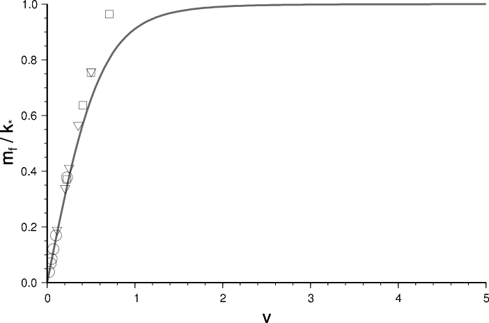
Figure 4: The slope, $\left.d\omega/dk\right|_{k=0}\equiv m_{f}/k_{*}$, as a function of $v\equiv m_{f}/\sqrt{2eB}$. The symbols show $m_{f}/k_{*}$ as found by a global fit to Eq. (V) for $m_{f}=0.1,\;0.5\;{\rm and}\;1$ (circles, triangles and squares). The curve is a plot of Eq. (42) and there is good agreement with the global fit for small $v$ and for all $m_{f}$. The deviation at large $v$ may be due to numerical issues and departures from the fitting formula in Eq. (V).

For a fermion in a zero mode to escape the wall, it necessarily requires some additional energy to transition from the zero mode to an energy larger than $m_{f}$. The additional energy can be exponentially small for $k>k_{*}$ and hence these fermion zero modes are extremely fragile – even a small perturbation can knock out the particles in these modes. For weak perturbations, the particles will be ejected into the lowest non-zero ($n\neq 0$) modes which also have energy $\sim m_{f}$. The perturbation itself can be inhomogeneities in the magnetic field, string motion and curvature, or the interactions of particles outside and on the string.

The modified dispersion has consequences for the cosmology of superconducting strings, including the formation of stable vortons VilShe . In connection with the scenario of positron production by superconducting strings in the Milky Way Ferrer:2005xv , our analysis indicates that positrons will be produced at an energy comparable to their rest mass, or about 511 keV. Then the annihilation of these positrons with ambient electrons will also produce 511 keV $\gamma-$rays.

Appendix A Validity of the Thick Wall Approximation

We now evaluate the leading corrections to the thick wall approximation used in section IVC. To this end it is helpful to write the Hamiltonian in Eq. (22) in the form $H=H_{0}+V$. Here $H_{0}$ is the Hamiltonian with the replacement $m(x)\rightarrow m(x_{0})$ where $x_{0}=-k/(eB)$. The perturbation

$$V=\left(\begin{array}[]{cc}m(x)-m(x_{0})&0\\ 0&m(x_{0})-m(x)\end{array}\right)$$ (43)

may be further decomposed as $V=V_{1}+V_{2}+\ldots$ where

$$V_{1} = m^{\prime}(x_{0})(x-x_{0})\left(\begin{array}[]{cc}1&0\\ 0&-1\end{array}\right)$$ (46)

$$V_{2} = \frac{1}{2}m^{\prime\prime}(x_{0})(x-x_{0})^{2}\left(\begin{array}[]{cc}1&0\\ 0&-1\end{array}\right).$$ (49)

In the thick wall limit we expect that $m(x)$ is slowly varying so that $V_{2}$ is nominally smaller than $V_{1}$. However we will find that both perturbations have a comparable effect on the energy of the zero mode state.

The zeroth-order solution to $H$ is the thick wall approximation presented in section IVC. The perturbation $V_{1}$ does not perturb the energy of the zero mode to first order since $\langle{\rm zero}|V_{1}|{\rm zero}\rangle=0$. A straightforward calculation shows that the second order correction due to $V_{1}$ is

$$\omega^{(2)}_{{\rm zero}}=-\frac{m_{f}^{3}}{2e^{2}B^{2}}\tanh x_{0}{\rm sech}^{4}x_{0}.$$ (50)

To assess the accuracy of the zeroth-order solution, we note that

$$m_{f}-\omega_{B}^{0}\rightarrow 2m_{f}\exp(-2x_{0})\ ,\ \ x_{0}\rightarrow\infty$$ (51)

On the other hand the correction

$$\omega^{(2)}_{{\rm zero}}\rightarrow-m_{f}^{3}\exp(-4x_{0})/(2e^{2}B^{2})\ ,\ \ x_{0}\rightarrow\infty$$ (52)

Thus the perturbation is far smaller than the distance to the mass gap and may be considered negligible for $x_{0}\gg 1$. We would also like to ensure that the perturbation $\omega^{(2)}_{{\rm zero}}$ does not shift the zero mode energy outside the mass gap for $x_{0}\sim 1$ or $x_{0}\ll 1$. Therefore our criterion becomes $|\omega^{(2)}_{{\rm zero}}|\ll m_{f}$, which leads to the condition $m_{f}\ll eB$. If $V_{1}$ was the only perturbation we would conclude that the zeroth-order approximation is accurate when $x_{0}\gg 1$ or when $m_{0}\ll eB$.

However, we must also take into account the perturbation $V_{2}$. Although nominally smaller than $V_{1}$, $V_{2}$ perturbs the zero mode energy to first order and therefore has a more significant effect. The first order correction is

$$\omega^{(1)}_{{\rm zero}}=-\frac{m_{f}}{2eB}\exp(-2x_{0}).$$ (53)

Applying the same reasoning as for the second order correction we conclude that the perturbation $V_{2}$ is insignificant when either (i) $x_{0}\gg 1$ and $eB\gg 1$ or (ii) $eB\gg m_{f}$ and $eB\gg 1$. These conditions subsume the conditions for $V_{1}$ to be negligible and are therefore the conditions that must be satisfied for the validity of the thick wall approximation to the zero mode.

Appendix B From Weber to hypergeometric function

We can find the dispersion relation of the zero modes for a given magnetic field by finding the roots of Eq. (41) that satisfy $\omega<m_{f}$ for different values of $k$. For this purpose it is useful to consider the expansion of the Weber function in the complex plane in terms of the Kummer confluent hypergeometric function ${}_{1}F_{1}(a;\rho;z)$:

$$D_{\nu}(z)=\sqrt{\pi}2^{\nu/2}e^{-z^{2}/4}\times$$

$$\left\{\frac{{}_{1}F_{1}\left(-\frac{\nu}{2};\frac{1}{2};\frac{z^{2}}{2}\right)}{\Gamma\left(\frac{1}{2}-\frac{\nu}{2}\right)}-\sqrt{2}z\frac{{}_{1}F_{1}\left(\frac{1}{2}-\frac{\nu}{2};\frac{3}{2};\frac{z^{2}}{2}\right)}{\Gamma\left(-\frac{\nu}{2}\right)}\right\}.$$ (54)

This representation is valid along the entire real axis. Since it is simpler than any form we have found in the literature, we briefly sketch its derivation. We start by observing that the Weber Eq. (35) may be transformed to the confluent hypergeometric equation by changing to the independent variable $s=z^{2}/2$ and the dependent variable $\xi=e^{s/2}\chi_{1}$. By means of this transformation, which is valid for $z>0$, we obtain a confluent hypergeometric equation (morse, , p. 671) with parameters $a=-\nu/2$ and $b=1/2$. Thus we obtain the solution to Eq. (35)

$$D_{\nu}(z)=2^{\nu/2}e^{i\nu\pi/2}e^{-z^{2}/4}{\cal U}_{2}\left(-\frac{\nu}{2},\frac{1}{2},\frac{z^{2}}{2}\right)$$ (55)

Here ${\cal U}_{2}$ is a confluent hypergeometric function of the third kind (morse, , p. 612), which is well-behaved as $z\rightarrow\infty$, and the constant pre-factors have been inserted to be consistent with the usual convention (morse, , p. 1641). We may now use a well known joining formula (morse, , p. 673) relating ${\cal U}_{2}$ to the standard confluent hypergeometric function ${}_{1}F_{1}$ to obtain the final result (54).

So far, our derivation applies only to $z>0$, but we can see from the differential Eq. (35) that $D_{\nu}(z)$ is analytic at $z=0$, and, since the function ${}_{1}F_{1}$ is known to be analytic over the entire complex plane, we conclude that Eq. (54) holds along the entire real axis. We note that the standard treatises whittaker ; morse both arrive at the representation Eq. (54), valid for $z>0$, but offer a much more complicated continuation of it along the negative $z$-axis (see, for example, the asymptotic analysis in whittaker , sections 16.51 and 16.52, or the identical discussion by morse on p. 1641).

References

- (1) C. Caroli, P.G. de Gennes and J. Matricon, Phys. Lett. 9, 307 (1964).
- (2) R. Jackiw and P. Rossi, Nucl. Phys. B190, 681 (1981).
- (3) E. Witten, Nucl. Phys. B249, 557 (1984).
- (4) A. Vilenkin and E.P.S. Shellard, Cosmic Strings and other Topological Defects, Cambridge University Press (1994).
- (5) F. Ferrer and T. Vachaspati, Phys. Rev. Lett. 95, 261302 (2005).
- (6) P. Jean et al., Astron. Astrophys. 407, L55 (2003); Knödlseder et al., Astron. Astrophys. 411, L457 (2003).
- (7) S. M. Barr and A. M. Matheson, Phys. Lett. B 198, 146 (1987); Phys. Rev. D 39, 412 (1989).
- (8) U. Fano, Phys Rev 124, 1866 (1961).
- (9) E. J. Weinberg, Phys. Rev. D 24, 2669 (1981).
- (10) E. T. Whittaker and G. N. Watson, A Course of Modern Analysis, (Cambridge University Press, Cambridge, England, 1915).
- (11) P. M. Morse and H. Feshbach, Methods of Theoretical Physics, (Mc Graw-Hill, New York, 1953).