Semi-classical stability of AdS NUT instantons

Abstract

The semi-classical stability of several AdS NUT instantons is studied. Throughout, the notion of stability is that of stability at the one-loop level of Euclidean Quantum Gravity. Instabilities manifest themselves as negative eigenmodes of a modified Lichnerowicz Laplacian acting on the transverse traceless perturbations. An instability is found for one branch of the AdS-Taub-Bolt family of metrics and it is argued that the other branch is stable. It is also argued that the AdS-Taub-NUT family of metrics are stable. A component of the continuous spectrum of the modified Lichnerowicz operator on all three families of metrics is found.

1 Introduction

Motivated by the AdS/CFT conjecture [1], there has recently been much interest in the two parameter AdS-Taub-NUT family of Riemannian biaxial Bianchi-IX metrics satisfying the Einstein equations with negative cosmological constant and non-trivial NUT charge [2, 3, 4, 5, 6, 7].

Upon the imposition of a regularity condition such metrics divide into two one parameter classes. The first class (AdS-Taub-Nut) have self-dual Weyl tensor and contain a nut. The second class of solutions (AdS-Taub-Bolt) contain a bolt, this class splits further into two branches. This is analogous to the case of AdS-Schwarzschild solutions at a given temperature, where the rôle of AdS is played by the AdS-Taub-Nut. The AdS-Schwarzshild solution with a smaller mass (and smaller horizon) is unstable and it’s action is greater than that of both AdS and the other AdS-Schwarzshild [8, 9]. We find a similar situation for AdS-Taub-Bolt.

In [4], Hartnoll and Kumar conjectured, based on the Klebanov-Polyakov version of the AdS₄/CFT₃ correspondence, that the global minimiser of the action for the AdS-Taub-NUT class of metrics should be stable. In [10], the stability of some of these spaces against scalar perturbations and brane nucleation was discussed. By considering a one-loop correction to the bulk gravitational partition function, we shall investigate the semi-classical linear stability of such spacetimes, using techniques developed by Hu [11] and applied to the case of Euclidean Taub-Bolt by Young [12]. These techniques have also been applied to the case of Lorentzian Taub-NUT recently by Holzegel [13]. The criterion for instability is that the modified Lichnerowicz operator

$$\widetilde{\Delta}_{L}h_{ab}=-\nabla^{e}\nabla_{e}h_{ab}-2R_{acbd}h^{cd}$$ (1)

acting on transverse, trace-free symmetric tensors should have no negative eigenmodes. We shall investigate the spectrum of this operator on metric perturbations of the AdS-Taub- instantons which preserve the $SU(2)$ symmetry. We find a negative mode for one of the instantons indicating instability for all values of the cosmological constant. We also find part of the positive spectrum of the modified Lichnerowicz operator for all instantons in the class under consideration.

In Section 2, we give a brief overview of the AdS-Taub-Nut and AdS-Taub-Bolt spaces, stating some results which we will later require. In Section 3, we introduce the method used to examine the stability of the spaces and we present an instability for one branch of the AdS-Taub-Bolt spaces and argue that the other spaces are linearly stable. In section 4 we present an alternative viewpoint, confirming the claims of section 3. In Section 5 we investigate the continuous spectrum of the operator $\widetilde{\Delta}_{L}$.

2 NUTs and Bolts in AdS space

The metric for both AdS-Taub-Nut and AdS-Taub-Bolt in four dimensions can be put into the form:

$$ds^{2}=\frac{1}{A(r)}dr^{2}+4N^{2}A(r)\sigma_{3}^{2}+B(r)(\sigma_{1}^{2}+\sigma_{2}^{2}),$$ (2)

where $\sigma_{i}$ are the left-invariant $SU(2)$ one-forms. The functions $A(r)$ and $B(r)$ are given by

$$A(r) = \frac{r^{2}+N^{2}-2mr+\ell^{-2}(r^{4}-6N^{2}r^{2}-3N^{4})}{r^{2}-N^{2}},$$

$$B(r) = r^{2}-N^{2},$$ (3)

where $N$ is the NUT charge and $m$ is the mass. This metric is Einstein, with $R_{\mu\nu}=-\frac{3}{\ell^{2}}g_{\mu\nu}$. The fixed point set of the $U(1)$ action is given by the solutions, $r=r_{+}$ of $A(r)=0$. If $B(r_{+})=0$, the fixed point set is of zero dimension and is known as a nut. If $B(r_{+})\neq 0$, the fixed point set is two dimensional and is known as a bolt. As $r$ approaches $r_{+}$, we will in general have a conical singularity unless $A(r)$ satisfies the regularity condition

$$\left|A^{\prime}(r_{+})\right|=\frac{1}{2N}.$$ (4)

This amounts to a relation between $m$ and $N$, which can be solved and we find that the number of solutions depends on the value of $\frac{\ell}{N}$.

For all values of $N$ and $\ell$ there is a solution, called the AdS-Taub-Nut solution where

$$r_{n}=N,\qquad m_{n}=\frac{N(\ell^{2}-4N^{2})}{\ell^{2}}.$$ (5)

Clearly we have $B(N)=0$, so we have a regular nut at $r=r_{n}$. We can also find two bolt solutions, which I shall call the AdS-Taub-Bolt^± solutions. They are given by:

$$r_{b\pm}=\frac{\ell^{2}\pm\sqrt{\ell^{4}-48N^{2}\ell^{2}+144N^{4}}}{12N},$$

$$m_{b\pm}=\frac{r_{b\pm}^{4}+(\ell^{2}-6N^{2})r_{b\pm}^{2}+N^{2}(\ell^{2}-3N^{2})}{2\ell^{2}r_{b\pm}}.$$ (6)

Clearly these equations only make sense if the quantity under the square root in the first equation is positive. This restricts $\ell/N$ to the range

$$\frac{\ell}{N}\geq 2\sqrt{3(2+\sqrt{3})}\approx 6.69.$$ (7)

Thus we find that requiring that the metric (2) be regular restricts the freedom quite considerably. For any given value of $\frac{\ell}{N}$, there are either $1$ or $3$ regular metrics in this family, excluding the critical case where $r_{\mathrm{b}+}=r_{\mathrm{b}-}$. It is possible to calculate the action for these spaces, but we shall postpone this until section 4.

It is useful to consider the limit $\ell\to\infty$, as we expect to recover the Euclidean Taub-NUT and Taub-Bolt solutions. For the AdS-Taub-Bolt⁺ case, this limit does not exist as $r_{\mathrm{b}+}\to\infty$ as $\ell$ gets large. However, for the other two cases we can take this limit and we find for the nut case:

$$m_{n}\to N,\hskip 56.9055ptA(r)\to\frac{r-N}{r+N},$$ (8)

which gives the well known form of the metric for the self-dual Taub-NUT instanton. For the AdS-Taub-Bolt^- case, we find:

$$r_{\mathrm{b}-}\to 2N,\hskip 28.45274ptm_{b-}\to\frac{5}{4}N,\hskip 28.45274ptA(r)\to\frac{r^{2}-\frac{5}{2}Nr+N^{2}}{r^{2}-N^{2}},$$ (9)

which gives the metric for Euclidean Taub-Bolt. This will provide a useful check on our stability results as for vanishing $\Lambda$, Taub-NUT has a self-dual Riemann tensor, and hence is linearly stable [14]. In [12] an unstable mode for the Taub-Bolt instanton was found.

3 Stability

3.1 A criterion for instability

Instabilities of a physical system may make themselves known as an imaginary part of the partition function for the system [15, 16]. The partition function for Euclidean quantum gravity is given by:

$$Z=\int\rmd[g]\rme^{-S[g]},$$ (10)

where the integral is taken over all Riemannian metrics subject to appropriate boundary behaviour and periodic in Euclidean time. The Euclidean action is given by:

$$S[g]=-\frac{1}{16\pi G}\int_{\mathcal{M}}\rmd V\sqrt{g}\left(R-2\Lambda\right)-\frac{1}{8\pi G}\int_{\partial\mathcal{M}}\rmd S\sqrt{h}K.$$ (11)

Unfortunately this is not positive definite. Under a conformal transformation of the metric, $g^{\prime}=\Omega^{2}g$, where for simplicity we assume $\Omega=1$ on a neigbourhood of $\partial\mathcal{M}$ the scalar curvature transforms like:

$$R^{\prime}=\Omega^{-2}R-6\Omega^{-3}\nabla^{a}\nabla_{a}\Omega.$$ (12)

Thus we find

$$I[g^{\prime}]=-\frac{1}{16\pi G}\int_{\mathcal{M}}\rmd V\sqrt{g}\left(\Omega^{2}R+6\Omega_{,a}\Omega^{,a}\right)-\frac{1}{8\pi G}\int_{\partial\mathcal{M}}\rmd S\sqrt{h}K.$$ (13)

So by taking $\Omega$ to vary quickly, we can make $I[g^{\prime}]$ as negative as we choose. This problem can be circumvented by an appropriate choice of contour, but only in the semi-classical (one-loop) approximation [17]. For a semi-classical approximation, we expand the integral (10) about the critical points of $S[g]$, where we expect the dominant contributions to the integral. These satisfy

$$\frac{\delta S}{\delta g_{ab}}=0\rightarrow R_{ab}=\Lambda g_{ab},$$

i.e., the classical Riemannian vacuum Einstein equations. Thus in order to find the semi-classical approximation to $Z$, one expands in small perturbations about the classical solutions:

$$\tilde{g}_{ab} = g_{ab}+h_{ab},$$

$$S[\tilde{g}] = S_{0}[g]+S_{2}[h]+O(h^{3}),$$ (14)

where $S_{2}[h]$ is second order in the small perturbation $h_{ab}$. We truncate the series for $I[\tilde{g}]$ and integrate over $h_{ab}$ to get

$$Z\cong Z_{1\hskip 1.42271pt\mathrm{loop}}=N\rme^{-S_{0}[g]}\int\rmd[h]\rme^{-S_{2}[h]},$$ (15)

where the integral is to be taken over physically distinct perturbations $h_{ab}$. The action $S_{2}[h]$ is invariant under gauge transformations which correspond to infinitesimal diffeomorphisms:

$$h_{ab}^{\prime}=h_{ab}+\nabla_{a}V_{b}+\nabla_{b}V_{a}.$$

In order to deal with this, we follow [18] and use the Fadeev-Popov gauge fixing technique. The gauge fixing condition will be:

$$\nabla_{a}\left(h^{ab}-\frac{1}{\beta}g^{ab}h\right)=W^{b},$$ (16)

where $W$ is an arbitrary vector, $\beta$ is an arbitrary constant and $h=h^{a}{}_{a}$ is the trace of the perturbation. The standard Fadeev-Popov method allows us to re-write the functional integral (15) as an integral over all fields $h_{ab}$, but with an altered integrand:

$$Z_{1\hskip 1.42271pt\mathrm{loop}}=N\rme^{-S_{0}[g]}\int\rmd[h](\mathrm{det}\ C)\rme^{-I_{2\hskip 1.42271pt\mathrm{eff.}}[h]}.$$ (17)

We now decompose the metric perturbation into a transverse, traceless part $\phi_{ab}$, a longitudinal traceless part generated by the vector $\tilde{n}$ and the trace $h$. Further, a Hodge-de Rham decomposition can be performed on $\tilde{n}$ so that

$$\tilde{n}_{a}=\eta_{a}+\nabla_{a}\chi,\hskip 14.22636pt\hbox{with}\hskip 14.22636pt\nabla_{a}\eta^{a}=0.$$

We can then write the effective action as:

$$I_{2\hskip 1.42271pt\mathrm{eff.}}=-\frac{1}{16\pi}\int\rmd V\mathcal{L}_{2},$$ (18)

with

$$\mathcal{L}_{2}=-\frac{1}{4}\phi^{ab}G_{abcd}\phi^{cd}+\frac{1}{2}hFh-2\gamma D^{ab}(\chi)D_{ab}(F\chi)-\gamma\mathfrak{D}^{abe}(\eta_{e})\mathfrak{D}_{abf}((C_{2})^{fd}\eta_{d})$$ (19)

where $\gamma$ is a constant related to $\beta$ by $\beta=4\gamma/(1+\gamma)$ and we have defined operators

$$F = \frac{1-3\gamma}{16\gamma}\nabla_{e}\nabla^{e}-\frac{1}{4}\Lambda,$$

$$D_{ab} = 2\nabla_{a}\nabla_{b}-\frac{1}{2}g_{ab}\nabla_{e}\nabla^{e},$$

$$\mathfrak{D}_{abe}(V^{e}) = \frac{1}{2}\left(\nabla_{a}V_{b}+\nabla_{b}V_{a}\right),$$

$$(C_{2})_{ab}V^{b} = -\left(\nabla_{e}\nabla^{e}+\Lambda\right)V_{a},$$

$$G_{abcd}\phi^{cd} = -\nabla_{e}\nabla^{e}\phi_{ab}-2R_{acbd}\phi^{cd},$$ (20)

where $V$ is a divergence free vector. It is possible to write the $(\mathrm{det}\ C)$ factor in (17) as a functional integral over anti-commuting vectors. Applying a Hodge-de Rham decomposition one finds

$$(\mathrm{det}\ C)\sim(\mathrm{det}\ C_{2})(\mathrm{det}\ F).$$

Finally, evaluating the Gaussian integrals in (17) we find

$$Z_{1\hskip 1.42271pt\mathrm{loop}}\sim(\mathrm{det}\ G)^{-\frac{1}{2}}(\mathrm{det}\ C_{2})^{\frac{1}{2}}.$$ (21)

Any zero modes of the determinants in (21) should be projected out. The determinants can be regularised by a $\zeta$-function regularisation [18]. $C_{2}$ is a positive semi-definite operator on the space of divergence free vector fields, with zero modes corresponding to Killing vectors. $G$ however is not positive definite and can in fact have a negative eigenmode. Such a negative eigenmode would introduce an imaginary part to the partition function and thus herald an instability. For example the flat Schwarzschild solution has a negative eigenmode. It is to be expected that the partition function be pathological in this case since the canonical ensemble for black holes breaks down due to the fact that they have negative specific heat.

Thus in our search for instabilities we can restrict to perturbations $h_{ab}$ which are transverse and tracefree. Our criterion for instabilities is that there exist negative eigenvalue solutions to the eigenvalue equation:

$$(\Delta_{L}h)_{ab}-2\Lambda h_{ab}=-\nabla_{e}\nabla^{e}h_{ab}-2R_{acbd}h^{cd}=\lambda h_{ab},$$ (22)

where we have re-expressed $G$ in terms of the Lichnerowicz Laplacian $\Delta_{L}$ [19]. This equation is consistent with the Transverse Traceless condition.

A negative eigenmode of (22) corresponds to a direction within the space of gauge fixed metric perturbations along which the classical solution $g_{ab}$ is a local maximum. The criterion that

$$\widetilde{\Delta}_{L}~{}=~{}\Delta_{L}~{}-~{}2\Lambda~{}\geq 0$$

for stability may be arrived at from a more geometric perspective (see for example Besse [20]) which avoids the Fadeev-Popov procedure used above. There are some cases in which it can be shown that $\widetilde{\Delta}_{L}$ is positive definite. These include the case when $g_{ab}$ has self-dual Riemann tensor (sometimes called the half-flat condition) [14] and also the case where $g_{ab}$ is Einstein-Kähler [21]. In both these cases, the existence of a covariantly constant spinor is used to relate the eigenmodes of $\widetilde{\Delta}_{L}$ to those of scalar Laplacians acting on charged fields.

3.2 Hu’s Technique

Hu [11] proposed a method for separation of variables of tensor equations in a homogeneous space where the metric can be written in the form

$$ds^{2}=dr^{2}+\overline{\gamma_{ij}}\sigma^{i}\sigma^{j},$$ (23)

where $i,j=1,2,3$ and $\sigma^{i}=\sigma_{i}$ are again the left invariant one-forms on $SU(2)$. This was generalised by Young [12] to the case where $g_{00}$ is permitted to depend on $r$. The metric perturbation is expanded in terms of the Wigner functions, $\mathcal{D}_{KM}{}^{J}(\theta,\phi,\psi)$ which are the analogue on $S^{3}$ of the spherical harmonics $Y_{l,m}(\theta,\phi)$. We concentrate on diagonal metric perturbations with the lowest “angular momentum”, $J=M=K=0$. These are the perturbations which preserve $SU(2)$ symmetry. The resulting equations, along with the transverse and traceless conditions for the general metric form (2) are given in the Appendix.

We first consider the $11$ and $22$ equations. Taking the difference of (53) and (54) we find a second order differential equation for $Y=h_{11}-h_{22}$. We can put this into Schrödinger form:

$$-\frac{d^{2}\chi}{dr_{*}^{2}}+V(r_{*})\chi=\lambda\chi,\hskip 42.67912pt0\leq r_{*}<\infty,$$ (24)

via the substitutions $Y=f\chi$ and $dr=gdr_{*}$, for some suitable $f$ and $g$. When we do this, we find that $V(r(r_{*}))$ is a positive function for $r>r_{+}$, so that no normalizable solutions to (24) exist with $\lambda<0$. This means that in the search for a negative eigenmode of (22) we may set $h_{11}=h_{22}$.

We now consider the other diagonal mode. Setting $h_{11}=h_{22}$, we can use the constraint equations (57), (58) with the 00 equation (55) to decouple a second order differential equation in $h_{00}$ from the others. If we can solve this, we can find $h_{11}$, $h_{22}$ and $h_{33}$ from the constraint equations. Since (22) is consistent with the transverse traceless condition, we know that (57), (58) and (55) imply (53) and (56). This can be checked explicitly. The equation we decouple may be written:

$$a(r)h^{\prime\prime}_{00}+b(r)h^{\prime}_{00}+c(r)h_{00}=0,$$ (25)

where differentiation with respect to $r$ is denoted by a prime and the coefficients are given by:

$$a(r) = A,$$

$$b(r) = 3A^{\prime}+\frac{AB^{\prime}}{B}+\frac{B(A^{\prime 2}-2AA^{\prime\prime})}{BA^{\prime}-AB^{\prime}}-\frac{A}{B}\left(\frac{2AB^{\prime 2}-BA^{\prime}B^{\prime}-2ABB^{\prime\prime}}{BA^{\prime}-AB^{\prime}}\right),$$

$$c(r) = \lambda+\frac{A^{\prime 2}}{2A}+\frac{A^{\prime}B^{\prime}}{B}-\frac{AB^{\prime 2}}{B^{2}}+A^{\prime\prime}+\frac{3}{2A}\left(\frac{BA^{\prime}+AB^{\prime}}{BA^{\prime}-AB^{\prime}}\right)$$

$$\hskip 14.22636pt+\frac{BA^{\prime}B^{\prime}+2BAB^{\prime\prime}-2AB^{\prime 2}}{B^{2}}\left(\frac{2BA^{\prime}+AB^{\prime}}{BA^{\prime}-AB^{\prime}}\right),$$

the rest of this section will consist of an analysis of this equation.

3.3 AdS-Taub-Nut

In the case where $A(r)$ and $B(r)$ are given by (2) with (5) we can cast equation (25) into Schrödinger form (24) where $V$ is once again found to be positive on the range $r>r_{+}$. Thus for AdS-Taub-Nut we have checked all the possible TT perturbations with $J=K=M=0$ and found that none give negative eigenvalue solutions to (22), thus there is no linear instability due to perturbations of this type. This is in agreement with the result that the $\ell\to\infty$ limit yields a (linearly) stable metric.

One would normally expect the eigenvalues of a Laplacian operator to be bounded below by the most symmetric modes. In our case that would be the $SU(2)$ invariant modes. In the case of the scalar Laplacian acting on a space with metric given by (2) this can be seen explicitly:

$$-\nabla^{2}\phi = -\nabla^{2}\left(\phi^{K}(r)\mathcal{D}_{K}(\theta,\phi,\psi)\right)$$ (26)

$$= \left(-\nabla^{2}\phi^{K}(r)\right)\mathcal{D}_{K}(\theta,\phi,\psi)-2\left(\partial^{d}\phi^{K}(r)\right)\left(\partial_{d}\mathcal{D}_{K}(\theta,\phi,\psi)\right)$$

$$\quad-\phi^{K}(r)\nabla^{2}\mathcal{D}_{K}(\theta,\phi,\psi)$$

$$= \left(-\nabla^{2}\phi^{K}(r)\right)\mathcal{D}_{K}(\theta,\phi,\psi)+\phi^{K}(r)\left(-\nabla^{2}\mathcal{D}_{K}(\theta,\phi,\psi)\right).$$

It can be shown that $(-\nabla^{2}\mathcal{D}_{K})$ is positive for this metric form. This separation into a radial part and an angular part does not occur for the the Laplacian acting on symmetric tensors as there are extra terms introduced by the connection. It has not been possible to show explicitly that the $SU(2)$ invariant perturbations give a lower bound for $\widetilde{\Delta}_{L}$, but one would still expect this to be the case. Increasing the spin of the perturbation modes introduces a more rapidly varying angular dependence, which one would expect to increase the eigenvalues of $-\nabla^{2}$ and hence of $\widetilde{\Delta}_{L}$.

We therefore conjecture that $\widetilde{\Delta}_{L}$ is positive acting on all metric perturbations and thus that AdS-Taub-Nut is stable. This may be related to the fact that the Weyl tensor is self dual for the AdS-Taub-Nut space. In the Euclidean case, the full Riemann tensor is self-dual and this is known to imply stability [14].

3.4 AdS-Taub-Bolt^-

In the case of AdS-Taub-Bolt^-, when one changes (25) into Schrödinger form, one encounters a divergent potential. In order to proceed, we must use numerical integration techniques. If we make the substitution $r=xN$, we find that the equations depend on $N$ only through the ratio $\frac{\ell}{N}$. We can therefore scale $N$ out of the problem and set $N=1$ without loss of generality. We must now consider the singularity structure of the differential equation (25). In the region of interest to us, $r\geq r_{\mathrm{b}-}$, we find that the equation has 3 regular singular points, at $r_{\mathrm{b}-}$, $r_{\mathrm{int.}}$ and infinity, where $r_{\mathrm{b}-}<r_{\mathrm{int.}}<\infty$. Other singular points outside of the range of interest preclude the possibility of an analytic solution.

We consider first the regular singular point at $r=r_{\mathrm{b}-}$. Near to this point, the differential equation has the asymptotic form:

$$h^{\prime\prime}_{00}+\frac{4}{r-r_{\mathrm{b}-}}h^{\prime}_{00}+\frac{2}{(r-r_{\mathrm{b}-})^{2}}h_{00}=0.$$ (27)

Substituting $h_{00}\sim(r-r_{\mathrm{b}-})^{\alpha}$, we find the indicial equation

$$\alpha^{2}+3\alpha+2=0,$$

with solutions $\alpha=-1$ and $\alpha=-2$. Thus there are two independent solutions of (25) that behave like $(r-r_{\mathrm{b}-})^{-1}$ and $(r-r_{\mathrm{b}-})^{-2}$ as $r\to r_{\mathrm{b}-}$. We impose a normalisation condition on the perturbation modes given by

$$\int\rmd Vh_{ab}h^{ab}<\infty.$$ (28)

Using the constraint equations, we can show that the $h_{00}$ contribution dominates the integrand in a region just outside the bolt. Using the fact that $dV=\sqrt{g}d\psi d\theta d\phi dr$, where $\psi$, $\theta$ and $\phi$ are the usual Euler angles on $SU(2)$ and the form of the metric (2) with the constraint equations (57, 58) we can show that this integral coverges at $r=r_{\mathrm{b}-}$ if and only if $h_{00}\sim(r-r_{\mathrm{b}-})^{\beta}$ where $\beta>-3/2$. Thus only one of the two independent solutions at $r=r_{\mathrm{b}-}$ represents a normalisable perturbation – we must pick the solution that behaves like $h_{00}\sim(r-r_{\mathrm{b}-})^{-1}$ near $r=r_{\mathrm{b}-}$. This provides us with a stepping off condition for our numerical integration. We can perform a Frobenius expansion of the solution about the regular singular point and then use this to calculate $h_{00}$ and $h^{\prime}_{00}$ at $r=r_{\mathrm{b}-}+\epsilon$ where $\epsilon$ is some small number, taken to be $10^{-5}$. This deals with the first regular singular point.

It can be shown, by a similar method to that used above that $h_{00}$ and $h^{\prime}_{00}$ are bounded as $r\to r_{\mathrm{int.}}$, so no special considerations are required for the numerical integration through this point.

Finally we need to take account of the regular singular point at infinity. In the limit that $r\to\infty$, the differential equation has the asymptotic form

$$h^{\prime\prime}_{00}+\frac{12}{r}h^{\prime}_{00}+\frac{28+\ell^{2}\lambda}{r^{2}}h_{00}=0.$$ (29)

Substituting $h_{00}\sim r^{\alpha}$ we find the indicial equation:

$$\alpha^{2}+11\alpha+(28+\ell^{2}\lambda)=0,$$

with solutions

$$\alpha_{\pm}=\frac{-11\pm\sqrt{9-4\ell^{2}\lambda}}{2}.$$ (30)

Using the constraint equations, we find that the integrand of (28) is dominated by the contribution from $h_{33}\sim r^{6}h_{00}$. This translates to a requirement that $h_{00}\sim r^{\beta}$ with $\beta<-\frac{11}{2}$ in order that (28) is satisfied. So we see that only one of the two independent solutions at infinity will give a normalisable perturbation. We will need to match the normalisable solution at infinity to the normalisable solution at $r_{\mathrm{b}+}$ and this matching, if it is possible, will determine the value of $\lambda$.

In order to ascertain whether there exist negative solutions for $\lambda$, we perform a numerical integration starting at $r_{\mathrm{b}-}+\epsilon$, with initial conditions determined from the Frobenius expansion about $r_{\mathrm{b}-}$. This determines the solution, up to a arbitrary multiplicative constant as we can determine $h_{00}$ and all its derivatives here. Having chosen the normalisable solution at the bolt, we need to check that the solution is normalisable at infinity. The only parameter we still have available is $\lambda$. As $r\to\infty$ the solution must have the asymptotic form found above, but will in general be a linear combination of the two independent asymptotic forms.

$$h_{00}(r)\sim k(\lambda)r^{\alpha_{+}}+l(\lambda)r^{\alpha_{-}},$$ (31)

where $\alpha_{+}>-11/2$ and $\alpha_{-}<-11/2$ are given in equation (30) and $k(\lambda),l(\lambda)$ are constants, which we assume to depend continuously on $\lambda$. The normalisation condition requires that $\lambda=\lambda_{0}$, where $k(\lambda_{0})=0$. Since we are only performing a numerical integration, it is not possible to find the form of $k(\lambda)$ explicitly, but we can find an interval within which $\lambda_{0}$ must lie.

If we consider $f(r)=r^{11/2}h_{00}(r)$, then $f(r)$ will generically tend to either positive or negative infinity, depending on the sign of $k(\lambda)$. If we can find numbers $\lambda_{1}$ and $\lambda_{2}$ such that $k(\lambda_{1})$ has opposite sign to $k(\lambda_{2})$, then we can deduce the existence of a root of $k(\lambda)$ in the interval $(\lambda_{1},\lambda_{2})$, by the Intermediate Value Theorem. This procedure was implemented using the computer package Mathematica, and negative eigenvalues have been found for values of $\ell$ on the entire range $2\sqrt{3(2+\sqrt{3})}<\ell<\infty$. A plot of these negative eigenvalues is shown in Figure 1, together with a best fit curve.

Figure 1: A plot showing the negative eigenvalue, $\lambda$, against $\ell$ for AdS-Taub-Bolt^- Space

We find that as $\ell\to\infty$, we have that $\lambda\to-0.20$ approximately. This is consistent with the findings of Roberta Young [12], who found that Euclidean Taub-Bolt had a negative eigenmode in this sector with $\lambda\approx-0.20$. We also find that as $\ell$ approaches the critical value where the AdS-Taub-Bolt^- and AdS-Taub-Bolt⁺ spaces are the same, the negative eigenvalue tends to zero from below.

3.5 AdS-Taub-Bolt⁺

The final case, where the bolt is located at $r=r_{\mathrm{b}+}$ is similar in many ways to the previous case. We find the same singularity structure and asymptotic forms for the perturbation. We can proceed in exactly the same way as above, but we find no negative eigenvalues. We therefore conjecture that this spacetime is stable, as it appears to have no negative eigenmodes in the lowest “angular momentum” state.

Figure 2: A plot showing the actions $S-S_{NUT}$ against $\ell$ for $N=1$

In Figure 2 we show a plot of the action of both AdS-Taub-Bolt spaces against $\ell$, with the action for AdS-Taub-Nut subtracted. This will be calculated in Section 4. The dotted line represents the unstable AdS-Taub-Bolt^- space, the horizontal axis the Taub-NUT space and the other curve AdS-Taub-Bolt⁺. The thicker line denotes the global minimizer of the action. We see here two interesting features. Firstly we note that at $\ell=2\sqrt{3(2+\sqrt{3})}$ we have a bifurcation, with the two Bolt families appearing, with one stable and the other unstable. We also note that at $\ell=2\sqrt{7+2\sqrt{10}}$ there is a phase transition from AdS-Taub-Nut as the global minimiser of the action to AdS-Taub-Bolt⁺ as the global minimiser. This is the NUT charged version of the Hawking-Page transition for AdS Black Holes [8].

4 Another Perspective on Stability

We will now present an alternative argument, which reproduces all the features of the plot in Figure 2.

In constructing the nut charged AdS instantons considered above, the usual technique (outlined in Section 2) is to consider a metric of the form (2) which satisfies the Einstein equations $R_{\mu\nu}=-\frac{3}{\ell^{2}}g_{\mu\nu}$. Then one imposes the condition of regularity to reduce the number of solutions to those given above. Here we shall consider a family of metrics which are regular everywhere, with a bolt (or possibly nut) located at $r_{b}$, which is treated as a free parameter. The AdS-Taub-Nut and Taub-Bolt($\pm$)-AdS instantons correspond to particular choices of $r_{b}$. We can then calculate the action for this family of spacetimes as a function of $r_{b}$ and we expect it will be locally extremized at the already known values of $r_{b}$ which give solutions of the Einstein equations. This corresponds to taking a slice parameterised by $r_{b}$ through the space of metrics containing a bolt or a nut.

Our metric ansatz will be:

$$ds^{2}=\frac{1}{A(r)}dr^{2}+4N^{2}A(r)\sigma_{3}^{2}+B(r)(\sigma_{1}^{2}+\sigma_{2}^{2}),$$ (32)

with

$$A(r) = \frac{(r-r_{b})(\alpha r+\beta+\ell^{-2}(r^{3}+r^{2}r_{b}))}{r^{2}-N^{2}},$$

$$B(r) = r^{2}-N^{2}.$$

We then impose regularity at $r=r_{b}$ and require the mass to be $m$, by considering the asymptotics. This gives us the metric functions:

$$A(r) = \frac{\left(r-r_{b}\right)\left(4N\left(r-r_{b}\right)r_{b}{\left(r+r_{b}\right)}^{2}-\ell^{2}\left(4mN\left(r_{b}-r\right)+\left(r+rb\right)\left(n^{2}-r_{b}^{2}\right)\right)\right)}{4\ell^{2}N\left(r^{2}-N^{2}\right)r_{b}},$$

$$B(r) = r^{2}-N^{2}.$$ (33)

We are now ready to calculate the action. The Euclidean action is given by:

$$S=S_{\mathrm{bulk}}+S_{\mathrm{surf.}}=-\frac{1}{16\pi G}\int_{\mathcal{M}}\rmd V\sqrt{g}\left(R+\frac{6}{\ell^{2}}\right)-\frac{1}{8\pi G}\int_{\partial\mathcal{M}}\rmd S\sqrt{h}K,$$ (34)

which is the standard Einstein-Hilbert action together with the Gibbons-Hawking-York boundary term. It is well known that this integral does not converge and so some means of regularising the action is required. The method used was that of counterterm subtraction proposed by Emparan, Johnson and Myers [22]. This was also found independently by Mann [23]. The calculation proceeds much as their calculation for the action of Taub-NUT. We find that the action of the metric defined by (32) and (33) is:

$$S=\frac{4N}{\ell^{2}}\left(r_{b}^{3}-3N^{2}r_{b}\right)+N^{2}+4Nr_{b}-r_{b}^{2}.$$ (35)

We note that this does not depend on $m$, which is also a free parameter of this family of metrics. The variation of this reduced action alone will not determine $m$, for that we require the full Einstein equations, which force $m$ to take the NUT or Bolt values at the critical points. Setting $r_{b}=xN$,defining $\mu=\ell/N$, and using the additive freedom to set $S=0$ for AdS-Taub-Nut we find

$$\frac{S}{N^{2}}=\frac{4}{\mu^{2}}(x^{3}-3x+2)-3+4x-x^{2}.$$

Figure 3: A plot showing $S/N^{2}$ against $x$ for several values of $\mu=\ell/N$

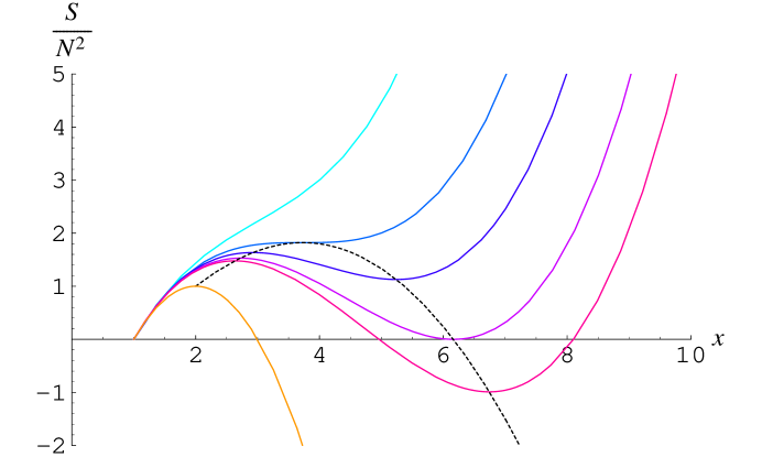
So we see that as $\mu$ is varied, the graph of $S/N^{2}$ will change. A plot of $S/N^{2}$ against $x$ for various values of $\mu$ is shown in Figure 3. Also included is a dotted curve showing the locus of the extremal points of the function as $\mu$ varies. We see that the point $x=1$, which corresponds to AdS-Taub-Nut is always a minimum since we must exclude the region $x<1$ from consideration as these metrics are not regular. For small $\mu$ this is the only minimum. As we increase $\mu$, we find that a pair of extrema, one maximum and one minimum appear at $\mu=\mu_{1}$, where

$$\mu_{1}=2\sqrt{3(2+\sqrt{3})},$$ (36)

which is precisely the value we would expect from the standard constructions for AdS-Taub-Nut and AdS-Taub-Bolt. If we think of this function $S(x)/N^{2}$ as defining the dynamics of some system by

$$\ddot{x}=-S^{\prime}(x)/N^{2},$$

then this bifurcation is of the form known as a saddle-node bifurcation, since it produces two new fixed points, one stable (a node) and one unstable (a saddle). Of course we have no formal dynamics on the space of metrics, but we still expect a local maximum to correspond to an unstable metric as it corresponds to a direction contributing an imaginary part to the partition function. Thus we shall refer to this bifurcation as a saddle-node bifurcation. We also find that the maximum occurs at precisely $x=r_{\mathrm{b}-}/N$ and the minimum at $x=r_{\mathrm{b}+}/N$, confirming our previous result that we expect the AdS-Taub-Bolt^- instanton to be unstable while the AdS-Taub-Bolt⁺ instanton is stable.

We also note a global bifurcation when $\mu=\mu_{2}$ where

$$\mu_{2}=2\sqrt{7+2\sqrt{10}},$$ (37)

when the global minimum moves from $x=1$ to $x=r_{\mathrm{b}+}/N$, which corresponds to AdS-Taub-Bolt⁺. This again accords with what we expect from previous analysis and corresponds to the Hawking-Page type phase transition.

These observations accord nicely with the general argument given in section 6 of [24] for the production of negative modes of the Lichnerowicz operator at bifurcation points in parameter space, in particular, from figure 1 we find that the negative eigenmode tends to zero as we approach the bifurcation.

Unfortunately this analysis cannot replace that of the previous section, since we have not explicitly found a normalisable negative mode of (22) for a perturbation about the AdS-Taub-Bolt^- instanton. It is possible to find the linearised perturbation of the metric at this point using our analysis, but this perturbation is not normalisable. It is however not in the Transverse, Tracefree gauge and it is possible that in the appropriate gauge this perturbation does give a normalisable mode.

5 The Continuous Spectrum of $\widetilde{\Delta}_{L}$

We have been so far concerned with looking for eigenvalues of $\widetilde{\Delta}_{L}$ on the AdS-Taub-Nut and -Bolt instantons. In the case of an elliptic operator on a non-compact manifold, the spectrum may also include a continuum of approximate eigenvalues. As an example, the time independent Schrödinger operator for the Hydrogen atom is a Laplacian type operator acting on $\mathbb{R}^{3}/\{0\}$. As is well known, this has a countable set of negative eigenvalues corresponding to the bound states. The spectrum however includes a continuum of positive “eigenvalues” which correspond to free particles moving in the Coulomb potential. These are not true eigenvalues since they do not correspond to normalisable eigenfunctions (wavefunctions). The sense in which they may be considered part of the spectrum is given below. We shall show that the continuous spectrum of $\widetilde{\Delta}_{L}$ acting on any of the three spaces considered above includes the ray $\{\lambda\in\mathbb{R}:\lambda>9/4l^{2}\}$.

5.1 A Little Functional Analysis

We can think of the space of gauge fixed, finite metric perturbations as a Hilbert space, defined by:

$$\mathcal{H}=\{h_{ab}\in T^{*}\mathcal{M}\otimes_{S}T^{*}\mathcal{M}:\nabla^{a}h_{ab}=0,h^{a}{}_{a}=0,\int_{\mathcal{M}}h_{ab}h^{ab}\rmd V<\infty\},$$ (38)

with $L^{2}$ inner product given by

$$\langle h,k\rangle=\int_{\mathcal{M}}h_{ab}k^{ab}\rmd V.$$ (39)

$\widetilde{\Delta}_{L}$ is then a linear operator from $\mathcal{H}_{2}$ to $\mathcal{H}_{0}$, where by $\mathcal{H}_{i}$ we mean

$$\mathcal{H}_{i}=\{h_{ab}\in\mathcal{H}:\partial_{c_{1}}\ldots\partial_{c_{i}}h_{ab}\hskip 5.69046pt\makebox{exist and are continuous}\}.$$ (40)

$\mathcal{H}_{i}$ are dense subsets of $\mathcal{H}$ with respect to the norm topology, where the norm is defined as usual by:

$$\left\|h\right\|^{2}=\langle h,h\rangle=\int_{\mathcal{M}}h_{ab}h^{ab}\rmd V.$$ (41)

A linear operator $A:\mathcal{H}\to\mathcal{H}$ is said to be bounded if $\exists$ $k$ such that

$$\left\|Ax\right\|\leq k\left\|x\right\|,\qquad\forall x\in\mathcal{H},$$ (42)

an operator which is not bounded is unbounded. We define the spectrum of $A$, $\sigma(A)$ as follows:

$\lambda\notin\sigma(A)\iff$ the following properties hold:

1. $(A-\lambda I)^{-1}$ exists,

2. $(A-\lambda I)^{-1}$ is bounded,

3. $(A-\lambda I)^{-1}$ is densely defined (i.e. defined on a dense subset of $\mathcal{H}$).

The set of $\lambda$ such that $(A-\lambda I)^{-1}$ does not exist is called the point spectrum of $A$, $P\sigma(A)$. the set of $\lambda$ such that $(A-\lambda I)^{-1})$ is unbounded is called the continuous spectrum of $A$, $C\sigma(A)$. We shall not discuss the third condition.

Lemma 5.1.

Given $\lambda\notin P\sigma(A)$, if there exists a sequence $x_{n}\in\mathcal{H}$ such that

$$\frac{\left\|(A-\lambda I)x_{n}\right\|}{\left\|x_{n}\right\|}\to 0,\qquad\mathrm{as}\qquad n\to\infty,$$

then $\lambda\in C\sigma(A)$.

Proof.

Define $y_{n}=(A-\lambda I)x_{n}$, by assumption as $n\to\infty$

$$\frac{\left\|y_{n}\right\|}{\left\|(A-\lambda I)^{-1}y_{n}\right\|}\to 0\qquad\Rightarrow\qquad\frac{\left\|(A-\lambda I)^{-1}y_{n}\right\|}{\left\|y_{n}\right\|}\to\infty,$$

but this clearly cannot occur if $(A-\lambda I)^{-1}$ is bounded, since if this is the case, $\exists$ $k$ such that

$$\frac{\left\|(A-\lambda I)^{-1}y_{n}\right\|}{\left\|y_{n}\right\|}\leq k.$$

Thus $(A-\lambda I)^{-1}$ must be unbounded, hence $\lambda\in C\sigma(\lambda)$. ∎

5.2 The $\widetilde{\Delta}_{L}$ Operator

We now consider the continuous spectrum of $\widetilde{\Delta}_{L}$. We will restrict attention for the moment to perturbations of the form considered in section 3. These are generated by the $h_{00}$ component, which has to satisfy equation (25). We first define the functions $\rho_{n}(x)$ by:

$$\rho_{n}(x)=\left\{\begin{array}[]{ll}1&\textrm{if $r<n$}\\ 1-K\int_{n}^{r}\exp\left[-\frac{1}{(x-n)^{2}}-\frac{1}{(x-n-1)^{2}}\right]\rmd x&\textrm{if $n\leq r\leq n+1$ }\\ 0&\textrm{if $r>n+1$}\end{array}\right.$$ (43)

with $K$ chosen so that $\rho_{n}(n+1)=0$. These functions are everywhere smooth on the real line. For $\lambda>9/4l^{2}$ we define $f(r)$ to be the solution of (25) which gives a finite contribution to $\langle h,h\rangle$ at $r_{+}$. This generates a perturbation which satisfies

$$(\widetilde{\Delta}_{L}-\lambda I)h_{ab}=0.$$

However this $h_{ab}$ is not an element of $\mathcal{H}$ since as $r\to\infty$ we have

$$f(r)\sim pr^{-11/2}\cos(\alpha\log r)+qr^{-11/2}\sin(\alpha\log r),$$ (44)

where $\alpha=\frac{1}{2}\sqrt{4l^{2}\lambda-9}$ is a constant. We find that for large $r$, counting powers of $r$ gives:

$$h_{ab}h^{ab}\sqrt{g}\sim f^{2}r^{10}\sim\frac{1}{r},$$ (45)

so that $\langle h,h\rangle$ does not converge. We define $f_{n}(r)$ by

$$f_{n}(r)=\rho_{n}(\log r)f(r).$$ (46)

Setting $h_{00}=f_{n}$ generates a perturbation which we call $h^{n}_{ab}$ via the constraint equations and we claim that

$$\frac{\left\|(\widetilde{\Delta}_{L}-\lambda I)h^{n}_{ab}\right\|}{\left\|h^{n}_{ab}\right\|}\to 0,\qquad\mathrm{as}\quad n\to\infty.$$

It is easily seen that $\left\|h^{n}_{ab}\right\|\to\infty$ since the integral in $\left\|h^{n}_{ab}\right\|$ is bounded below by the integral for $\left\|h_{ab}\right\|$ cut off at $r=\rme^{n}$. It suffices then to show that $\left\|(\widetilde{\Delta}_{L}-\lambda I)h^{n}_{ab}\right\|$ is bounded as $n\to\infty$. Clearly $(\widetilde{\Delta}_{L}-\lambda I)h^{n}_{ab}=0$ on $\{r_{+}\leq r\leq\rme^{n}\}\cup\{\rme^{n+1}\leq r\}$ so we need to estimate

$$\int_{r=\rme^{n}}^{\rme^{n+1}}\left[\left(\widetilde{\Delta}_{L}-\lambda I\right)h^{n}\right]_{ab}\left[\left(\widetilde{\Delta}_{L}-\lambda I\right)h^{n}\right]^{ab}\rmd V=\left\|(\widetilde{\Delta}_{L}-\lambda I)h^{n}\right\|^{2},$$ (47)

for large $n$. In this limit, we can use the large $n$ asymptotic expansions to estimate the leading order behaviour of this term. Substituting these in, we find that:

$$\left\|(\widetilde{\Delta}_{L}-\lambda I)h^{n}\right\|^{2}\sim K\int_{\rme^{n}}^{\rme^{n+1}}(L\tilde{f}_{n})^{2}r^{10}\rmd r,$$ (48)

with

$$L\tilde{f}_{n}=r^{2}\tilde{f}^{\prime\prime}_{n}+12r\tilde{f}^{\prime}_{n}+(28+l^{2}\lambda)\tilde{f}_{n},$$ (49)

the leading order expansion of (25) and where $\tilde{f}_{n}$ is defined by:

$$\tilde{f}_{n}(r)=(pr^{-11/2}\cos(\alpha\log r)+qr^{-11/2}\sin(\alpha\log r))\rho_{n}(\log r).$$ (50)

Under a change of variables $x=\log r$ the integral in (48) becomes:

$$\int_{e^{n}}^{e^{n+1}}(L\tilde{f}_{n})^{2}r^{10}dr = \int_{n}^{n+1}\left\{\rho_{n}^{\prime\prime}(x)(p\sin\alpha x+q\cos\alpha x)+2\alpha\rho_{n}^{\prime}(x)(q\sin\alpha x-p\cos\alpha x)\right\}^{2}dx$$ (51)

$$= \int_{0}^{1}\left\{\rho_{0}^{\prime\prime}(y)(p\sin\alpha(y+n)+q\cos\alpha(y+n))\right.$$

$$\hskip 14.22636pt\left.+2\alpha\rho_{0}^{\prime}(y)(q\sin\alpha(y+n)-p\cos\alpha(y+n))\right\}^{2}dy,$$

since $\rho_{n}(x)=\rho_{0}(x-n)$. Now for all $n$ the integrand is bounded since

$$\left|\rho_{0}^{\prime}(x)\right| \leq 6,$$

$$\left|\rho_{0}^{\prime\prime}(x)\right| \leq 60,$$

thus there exist constants $C$ and $\tilde{n}$ such that

$$\left\|(\widetilde{\Delta}_{L}-\lambda I)h^{n}\right\|\leq C,\qquad\forall\quad n\geq\tilde{n}.$$ (52)

We can now apply lemma 5.1 to the operator $\widetilde{\Delta}_{L}$ and we find that for $\lambda>9/4l^{2}$, $(\widetilde{\Delta}_{L}-\lambda I)^{-1}$ is unbounded, hence $\{\lambda>9/4l^{2}\}\subseteq C\sigma(\widetilde{\Delta}_{L})$.

This result makes no use of the value of $m$ or the location of the zeroes of $A(r)$, so it holds for all three of the instantons considered here. It is also possible to perform this analysis for the other $SU(2)$ invariant modes of the perturbation and we find exactly the same condition on $\lambda$ in order that it be in the continuous spectrum.

6 Conclusions

We have studied the semi-classical stability of the AdS-Taub-Nut instantons and the two branch family of AdS-Taub-Bolt instantons and we have found a negative mode of (22) for the AdS-Taub-Bolt^- instanton, implying that this instanton is unstable. For the AdS-Taub-Nut and AdS-Taub-Bolt⁺ instanton we have argued that they are (linearly at least) stable. We have also justified this by considering a family of regular metrics, not necessarily satisfying Einstein’s equations, which contains these instantons as special cases. This gives an intuitive sense of how the saddle-node bifurcation in the $S-\mu$ plane arises, as well as the Hawking-Page type bifurcation which occurs. We have also found that for all three instantons the continuous spectrum includes the ray $\{\lambda>9/4l^{2}\}$.

Appendix

The following are a set of differential equations governing the $J=M=K=0$ piece of the tensor harmonic decomposition of the equation

$$-\nabla_{e}\nabla^{e}h_{ab}-2R_{acbd}h^{cd}=\lambda h_{ab},$$

for the metric

$$ds^{2}=\frac{1}{A(r)}dr^{2}+4N^{2}A(r)\sigma_{3}^{2}+B(r)(\sigma_{1}^{2}+\sigma_{2}^{2}).$$

We suppress the $r$ dependence of $A(r)$ and $B(r)$ and use a prime to denote differentiation with respect to $r$. These are taken from [12], with some typos corrected.

11 Component

$$\overline{a}(r)h^{\prime\prime}_{11}+\overline{b}(r)h^{\prime}_{11}+\overline{c}(r)h_{00}+\overline{d}(r)h_{11}+\overline{e}(r)h_{22}+\overline{f}(r)h_{33}=-\lambda h_{11},$$ (53)

with

$$\overline{a}(r) = A,$$

$$\overline{b}(r) = A^{\prime}-A\frac{B^{\prime}}{B},$$

$$\overline{c}(r) = -2A(A^{\prime}B^{\prime})+\frac{4A^{2}B^{\prime 2}}{B}-4A^{2}B^{\prime\prime},$$

$$\overline{d}(r) = \frac{2}{B}-\frac{AB^{\prime\prime}}{B}-\frac{A^{\prime}B^{\prime}}{B}+\frac{1}{2}A\left(\frac{B^{\prime}}{B}\right)^{2}-\frac{4N^{2}A}{B^{2}}-\frac{1}{2N^{2}A},$$

$$\overline{e}(r) = \frac{1}{2N^{2}A}-\frac{4N^{2}A}{B^{2}}-\frac{1}{2}A\left(\frac{B^{\prime}}{B}\right)^{2},$$

$$\overline{f}(r) = -\frac{A^{\prime}B^{\prime}}{8N^{2}A}+\frac{1}{B}.$$

22 Component

$$a(r)h^{\prime\prime}_{22}+b(r)h^{\prime}_{22}+c(r)h_{00}+d(r)h_{11}+e(r)h_{22}+f(r)h_{33}=-\lambda h_{22},$$ (54)

with

$$\begin{array}[]{rclcrcl}\displaystyle a(r)&=&\displaystyle\overline{a}(r),&&\displaystyle d(r)&=&\displaystyle\overline{e}(r),\\ \displaystyle b(r)&=&\displaystyle\overline{b}(r),&\hskip 28.45274pt\mbox{and}&\displaystyle e(r)&=&\displaystyle\overline{d}(r),\\ \displaystyle c(r)&=&\displaystyle\overline{c}(r),&&\displaystyle f(r)&=&\displaystyle\overline{f}(r).\\ \end{array}$$

Where the overbar denotes the coefficients for (53).

00 Component

$$a(r)h^{\prime\prime}_{00}+b(r)h^{\prime}_{00}+c(r)h_{00}+d(r)X+f(r)h_{33}=-\lambda h_{00},$$ (55)

with

$$a(r) = A,$$

$$b(r) = 3A^{\prime}+\frac{AB^{\prime}}{B},$$

$$c(r) = \frac{A^{\prime 2}}{2A}+\frac{A^{\prime}B^{\prime}}{B}-A\left(\frac{B^{\prime}}{B}\right)^{2}+A^{\prime\prime},$$

$$d(r) = -\frac{A^{\prime}B^{\prime}}{8AB^{2}}+\frac{B^{\prime 2}}{4B^{3}}-\frac{B^{\prime\prime}}{4B^{2}},$$

$$f(r) = \frac{A^{\prime 2}}{32N^{2}A^{3}}-\frac{A^{\prime\prime}}{16N^{2}A^{2}},$$

and $X=h_{11}+h_{22}$.

33 Component

$$a(r)h^{\prime\prime}_{33}+b(r)h^{\prime}_{33}+c(r)h_{00}+d(r)X+f(r)h_{33}=-\lambda h_{33},$$ (56)

with

$$a(r) = A,$$

$$b(r) = -A^{\prime}+\frac{AB^{\prime}}{B},$$

$$c(r) = 8N^{2}AA^{\prime 2}-16N^{2}A^{2}A^{\prime\prime},$$

$$d(r) = \frac{16N^{4}A^{2}}{B^{3}}-\frac{2N^{2}AA^{\prime}B^{\prime}}{B^{2}},$$

$$f(r) = -A^{\prime\prime}+\frac{A^{\prime 2}}{2A}-\frac{A^{\prime}B^{\prime}}{B}-\frac{4N^{2}A}{B^{2}},$$

and $X=h_{11}+h_{22}$.

Constraint Equations

The above system of equations is consistent with the transverse and tracefree conditions on $h_{ab}$. This gives us the constraint equation

$$Ah_{00}+\frac{1}{4B}(h_{11}+h_{22})+\frac{1}{16N^{2}A}h_{33}=0,$$ (57)

coming from the traceless condition $h^{a}{}_{a}=0$, and

$$Ah^{\prime}_{00}+\left(\frac{3}{2}A^{\prime}+\frac{AB^{\prime}}{B}\right)h_{00}-\frac{B^{\prime}}{8{B^{2}}}\left(h_{11}+h_{22}\right)-\frac{A^{\prime}}{32N^{2}A^{2}}h_{33}=0,$$ (58)

which comes from the transverse condition $\nabla_{a}h^{ab}=0$.

References

- [1] J. M. Maldacena, Adv. Theor. Math. Phys. 2 (1998) 231. [arXiv:hep-th/9711200].
- [2] M. M. Akbar, Nucl. Phys. B 663 (2003) 215. [arXiv:gr-qc/0301007].
- [3] M. M. Akbar and P. D. D’Eath, Nucl. Phys. B 648 (2003) 397 [arXiv:gr-qc/0202073].
- [4] S. A. Hartnoll and S. P. Kumar, JHEP 0506, 012 (2005). [arXiv:hep-th/0503238].
- [5] R. Clarkson, L. Fatibene and R. B. Mann, Nucl. Phys. B 652 (2003) 348. [arXiv:hep-th/0210280]
- [6] A. Chamblin, R. Emparan, C. V. Johnson and R. C. Myers, Phys. Rev. D 59, 064010 (1999) [arXiv:hep-th/9808177].
- [7] S. W. Hawking, C. J. Hunter and D. N. Page, Phys. Rev. D 59, 044033 (1999) [arXiv:hep-th/9809035].
- [8] S. W. Hawking and D. N. Page, Commun. Math. Phys. 87 (1983) 577.
- [9] T. Prestidge, Phys. Rev. D 61 (2000) 084002 [arXiv:hep-th/9907163].
- [10] M. Kleban, M. Porrati and R. Rabadan, JHEP 0508, 016 (2005) [arXiv:hep-th/0409242].
- [11] B. L. Hu, J. Math. Phys. 15 (1974) 1748.
- [12] R. E. Young, Phys. Rev. D 28, 2420 (1983).
- [13] G. H. Holzegel, [arXiv:gr-qc/0602045].
- [14] S. W. Hawking and C. N. Pope, Nucl. Phys. B 146 (1978) 381.
- [15] J. S. Langer, Annals Phys. 54 (1969) 258.
- [16] S. R. Coleman, in The Whys of Subnuclear Physics, Proceedings of the International School of Subnuclear Physics, Erice, 1977, edited by A. Zichichi (Plenum, New York, 1979).
- [17] G. W. Gibbons, S. W. Hawking and M. J. Perry, Nucl. Phys. B 138 (1978) 141.
- [18] G. W. Gibbons and M. J. Perry, Nucl. Phys. B 146 (1978) 90.
- [19] A. Lichnerowicz, Instutute des Hautes Etudes Scientifiques, Publications Mathématiques, 10 (1961)
- [20] A. L. Besse, Einstein Manifolds, Springer-Verlag, Berlin, 1987.
- [21] C. N. Pope, J. Phys. A 15 (1982) 2455.
- [22] R. Emparan, C. V. Johnson and R. C. Myers, Phys. Rev. D 60 (1999) 104001. [arXiv:hep-th/9903238].
- [23] R. B. Mann, Phys. Rev. D 60, 104047 (1999) [arXiv:hep-th/9903229].
- [24] G. W. Gibbons, S. A. Hartnoll and C. N. Pope, Phys. Rev. D 67 (2003) 084024 [arXiv:hep-th/0208031].